A Covariance Regression Model

Abstract

Classical regression analysis relates the expectation of a response variable to a linear combination of explanatory variables. In this article, we propose a covariance regression model that parameterizes the covariance matrix of a multivariate response vector as a parsimonious quadratic function of explanatory variables. The approach is analogous to the mean regression model, and is similar to a factor analysis model in which the factor loadings depend on the explanatory variables. Using a random-effects representation, parameter estimation for the model is straightforward using either an EM-algorithm or an MCMC approximation via Gibbs sampling. The proposed methodology provides a simple but flexible representation of heteroscedasticity across the levels of an explanatory variable, improves estimation of the mean function and gives better calibrated prediction regions when compared to a homoscedastic model.

Some key words: heteroscedasticity, positive definite cone, random effects.

1 Introduction

Estimation of a conditional mean function $\mbox{\boldmath{${\rm\mu}$}}_{\rm x}={\rm E}[\mbox{\boldmath{${\rm y}$}}|\mbox{\boldmath{${\rm x}$}}]$ is a well studied data-analysis task for which there are a large number of statistical models and procedures. Less studied is the problem of estimating a covariance function $\mbox{\boldmath{${\rm\Sigma}$}}_{\rm x}={\rm Var}[\mbox{\boldmath{${\rm y}$}}|\mbox{\boldmath{${\rm x}$}}]$ across a range of values for an explanatory ${\rm x}$-variable. In the univariate case, several procedures assume that the variance can be expressed as a function of the mean, i.e. $\sigma^{2}_{\rm x}=g(\mu_{\rm x})$ for some known function $g$ (see, for example, Carroll et al. (1982)). In many such cases the data can be represented by a generalized linear model with an appropriate variance function, or perhaps the data can be transformed to a scale for which the variance is constant as a function of the mean (Box and Cox, 1964). Other approaches separately parameterize the mean and variance, giving either a linear model for the standard deviation (Rutemiller and Bowers, 1968) or by forcing the variance to be non-negative via a link function (Smyth, 1989). In situations where the explanatory variable $x$ is continuous and the variance function is assumed to be smooth, Carroll (1982) and Müller and Stadtmüller (1987) propose and study kernel estimates of the variance function.

Models for multivariate heteroscedasticity have been developed in the context of multivariate time series, for which a variety of multivariate “autoregressive conditionally heteroscedastic” (ARCH) models have been studied (Engle and Kroner, 1995; Fong et al., 2006). However, the applicability of such models are limited to situations where the heteroscedasticity is temporal in nature. A recent approach by Yin et al. (2010) uses a kernel estimator to allow $\mbox{\boldmath{${\rm\Sigma}$}}_{\rm x}$ to vary smoothly with ${\rm x}$. However, their focus is on a single continuous univariate explanatory variable, and it is not clear how to generalize such an approach to allow for discrete or categorical predictors. For many applications, it would be desirable to construct a covariance function $\{\mbox{\boldmath{${\rm\Sigma}$}}_{\rm x}:\mbox{\boldmath{${\rm x}$}}\in\mathcal{X}\}$ for which the domain of the explanatory ${\rm x}$-variable is the same as in mean regression, that is, the explanatory vector can contain continuous, discrete and categorical variables. With this goal in mind, Chiu et al. (1996) suggested modeling the elements of the logarithm of the covariance matrix, $\mbox{\boldmath{${\rm\Phi}$}}_{\rm x}=\log\mbox{\boldmath{${\rm\Sigma}$}}_{\rm x}$, as linear functions of the explanatory variables, so that $\phi_{j,k,\rm_{x}}=\mbox{\boldmath{${\rm\beta}$}}_{j,k}^{T}\mbox{\boldmath{${\rm x}$}}$ for unknown coefficients $\mbox{\boldmath{${\rm\beta}$}}_{j,k}$. This approach makes use of the fact that the only constraint on $\mbox{\boldmath{${\rm\Phi}$}}_{\rm x}$ is that it is symmetric. However, as the authors note, parameter interpretation for this model is difficult: For example, a submatrix of $\mbox{\boldmath{${\rm\Sigma}$}}_{\rm x}$ is not generally the matrix exponential of the same submatrix of $\mbox{\boldmath{${\rm\Phi}$}}_{\rm x}$, and so the elements of $\mbox{\boldmath{${\rm\Phi}$}}_{\rm x}$ do not directly relate to the corresponding covariances in $\mbox{\boldmath{${\rm\Sigma}$}}_{\rm x}$. Additionally, the number of parameters in this model can be quite large: For $\mbox{\boldmath{${\rm y}$}}\in\mathbb{R}^{p}$ and $\mbox{\boldmath{${\rm x}$}}\in\mathbb{R}^{q}$, the model involves a separate $q$-dimensional vector of coefficients for each of the $p(p+1)/2$ unique elements of $\mbox{\boldmath{${\rm\Phi}$}}_{x}$, thus requiring $q\times p(p+1)/2$ parameters to be estimated.

Another clever reparameterization-based approach to covariance regression modeling was provided by Pourahmadi (1999), who suggested modeling the unconstrained elements of the Cholesky decomposition of $\mbox{\boldmath{${\rm\Sigma}$}}_{\rm x}^{-1}$ as linear functions of ${\rm x}$. The parameters in this model have a natural interpretation: The first $j-1$ parameters in the $j$th row of the Cholesky decomposition relate to the conditional distribution of $y_{j}$ given $y_{1},\ldots,y_{j-1}$. This model is not invariant to reorderings of the elements of ${\rm y}$, and so is most appropriate when there is a natural order to the variables, such as with longitudinal data. Like the logarithmic covariance model of Chiu et al. (1996), the general form of the Cholesky factorization model requires $q\times p(p+1)/2$ parameters to be estimated.

In this article we develop a simple parsimonious alternative to these reparameterization-based approaches. The covariance regression model we consider is based on an analogy with linear regression, and is given by $\mbox{\boldmath{${\rm\Sigma}$}}_{\rm x}=\mbox{\boldmath{${\rm\Psi}$}}+\mbox{\bf{B}}\mbox{\boldmath{${\rm x}$}}\mbox{\boldmath{${\rm x}$}}^{T}\mbox{\bf{B}}^{T}$, where ${\rm\Psi}$ is positive definite and B is a $p\times q$ real matrix. As a function of ${\rm x}$, $\mbox{\boldmath{${\rm\Sigma}$}}_{\rm x}$ is a curve within the cone of positive definite matrices. The $q\times p$ parameters of B have a direct interpretation in terms of how heteroscedasticity co-occurs among the $p$ variables of ${\rm y}$. Additionally, the model has a random-effects representation, allowing for straightforward maximum likelihood parameter estimation using the EM-algorithm, and Bayesian inference via Gibbs sampling. In the presence of heteroscedasticity, use of this covariance regression model can improve estimation of the mean function, characterize patterns of non-constant covariance and provide prediction regions that are better calibrated than regions provided by homoscedastic models.

A geometric interpretation of the proposed model is developed in Section 2, along with a representation as a random-effects model. Section 3 discusses methods of parameter estimation and inference, including an EM-algorithm for obtaining maximum likelihood estimates (MLEs), an approximation to the covariance matrix of the MLEs, and a Gibbs sampler for Bayesian inference. A simulation study is presented in Section 4 that evaluates the estimation error of the regression coefficients in the presence of heteroscedasticity, the power of a likelihood ratio test of heteroscedasticity, as well as the coverage rates for approximate confidence intervals for model parameters. Section 5 considers an extension of the basic model to accommodate more complex patterns of heteroscedasticity, and Section 6 illustrates the model in an analysis of bivariate data on children’s height and lung function. In this example it is shown that a covariance regression model provides better-calibrated prediction regions than a constant variance model. Section 7 provides a summary of the article.

2 A covariance regression model

Let $\mbox{\boldmath{${\rm y}$}}\in{\mathbb{R}}^{p}$ be a random multivariate response vector and $\mbox{\boldmath{${\rm x}$}}\in{\mathbb{R}}^{q}$ be a vector of explanatory variables. Our goal is to provide a parsimonious model and estimation method for ${\rm Cov}[\mbox{\boldmath{${\rm y}$}}|\mbox{\boldmath{${\rm x}$}}]=\mbox{\boldmath{${\rm\Sigma}$}}_{\rm x}$, the conditional covariance matrix of ${\rm y}$ given ${\rm x}$. We begin by analogy with linear regression. The simple linear regression model expresses the conditional mean $\mbox{\boldmath{${\rm\mu}$}}_{\rm x}={\rm E}[\mbox{\boldmath{${\rm y}$}}|\mbox{\boldmath{${\rm x}$}}]$ as $\mbox{\boldmath{${\rm b}$}}+\mbox{\bf{B}}\mbox{\boldmath{${\rm x}$}}$, an affine function of ${\rm x}$. This model restricts the $p$-dimensional vector $\mbox{\boldmath{${\rm\mu}$}}_{\rm x}$ to a $q$-dimensional subspace of $\mathbb{R}^{p}$. The set of $p\times p$ covariance matrices is the cone of positive semidefinite matrices. This cone is convex and thus closed under addition. The simplest version of our proposed covariance regression model expresses $\mbox{\boldmath{${\rm\Sigma}$}}_{\rm x}$ as

$$\mbox{\boldmath{${\rm\Sigma}$}}_{\rm x}=\mbox{\boldmath{${\rm\Psi}$}}+\mbox{\bf{B}}\mbox{\boldmath{${\rm x}$}}\mbox{\boldmath{${\rm x}$}}^{T}\mbox{\bf{B}}^{T},$$ (1)

where ${\rm\Psi}$ is a $p\times p$ positive-definite matrix and B is a $p\times q$ matrix. The resulting covariance function is positive definite for all ${\rm x}$, and expresses the covariance as equal to a “baseline” covariance matrix ${\rm\Psi}$ plus a rank-1, $p\times p$ positive definite matrix that depends on ${\rm x}$. The model given by Equation 1 is in some sense a natural generalization of mean regression to a model for covariance matrices. A vector mean function lies in a vector (linear) space, and is expressed as a linear map from $\mathbb{R}^{q}$ to $\mathbb{R}^{p}$. The covariance matrix function lies in the cone of positive definite matrices, where the natural group action is matrix multiplication on the left and right. The covariance regression model expresses the covariance function via such a map from the $q\times q$ cone to the $p\times p$ cone.

2.1 Model flexibility and geometry

Letting $\{\mbox{\boldmath{${\rm b}$}}_{1},\ldots,\mbox{\boldmath{${\rm b}$}}_{p}\}$ be the rows of B, the covariance regression model gives

$${\rm Var}[y_{j}|\mbox{\boldmath{${\rm x}$}}] = \psi_{j,j}+\mbox{\boldmath{${\rm b}$}}_{j}^{T}\mbox{\boldmath{${\rm x}$}}\mbox{\boldmath{${\rm x}$}}^{T}\mbox{\boldmath{${\rm b}$}}_{j}$$ (2)

$${\rm Cov}[y_{j},y_{k}|\mbox{\boldmath{${\rm x}$}}] = \psi_{j,k}+\mbox{\boldmath{${\rm b}$}}_{j}^{T}\mbox{\boldmath{${\rm x}$}}\mbox{\boldmath{${\rm x}$}}^{T}\mbox{\boldmath{${\rm b}$}}_{k}.$$ (3)

The parameterization of the variance suggests that the model requires the variance of each element of ${\rm y}$ to be increasing in the elements of ${\rm x}$, as the minimum variance is obtained when $\mbox{\boldmath{${\rm x}$}}=0$. This constraint can be alleviated by including an intercept term so that the first element of ${\rm x}$ is 1. For example, in the case of a single scalar explanatory variable $x$, we abuse notation slightly and write $\mbox{\boldmath{${\rm x}$}}=(1,x)^{T}$, $\mbox{\boldmath{${\rm b}$}}_{j}=(b_{0,j},b_{1,j})^{T}$, giving

$${\rm Var}[y_{j}|\mbox{\boldmath{${\rm x}$}}] = \psi_{j,j}+(b_{0,j}+b_{1,j}x)^{2}$$

$${\rm Cov}[y_{j},y_{k}|\mbox{\boldmath{${\rm x}$}}] = \psi_{j,k}+(b_{0,j}+b_{1,j}x)(b_{0,k}+b_{1,k}x).$$

For any given finite interval $(c,d)\subset\mathbb{R}$ there exist parameter values $(b_{0,j},b_{1,j})$ so that the variance of $y_{j}$ is either increasing or decreasing in $x$ for $x\in(c,d)$.

We now consider the geometry of the covariance regression model. For each ${\rm x}$, the model expresses $\mbox{\boldmath{${\rm\Sigma}$}}_{\rm x}$ as equal to a point ${\rm\Psi}$ inside the positive-definite cone plus a rank-1 positive-semidefinite matrix $\mbox{\bf{B}}\mbox{\boldmath{${\rm x}$}}\mbox{\boldmath{${\rm x}$}}^{T}\mbox{\bf{B}}^{T}$. The latter matrix is a point on the boundary of the cone, so the range of $\mbox{\boldmath{${\rm\Sigma}$}}_{\rm x}$ as a function of x can be seen as a submanifold of the boundary of the cone, but “pushed into” the cone by an amount ${\rm\Psi}$. Figure 1 represents this graphically for the simplest of cases, in which $p=2$ and there is just a single scalar explanatory variable $x$. In this case, each covariance matrix can be expressed as a three-dimensional vector $(\sigma_{1}^{2},\sigma_{2}^{2},\sigma_{1,2})$ such that

$$\sigma_{1}^{2}\geq 0\ ,\ \sigma^{2}_{2}\geq 0\ ,\ |\sigma_{1,2}|\leq\sigma_{1}\sigma_{2}.$$

The set of such points constitutes the positive semidefinite cone, whose boundary is shown by the outer surfaces in the two plots in Figure 1.

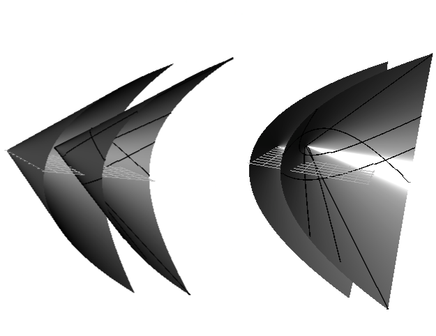
Figure 1: The positive-definite cone and a translation, from two perspectives. The outer surface is the boundary of the the positive definite cone, and the inner cone is equal to the boundary plus a positive definite matrix ${\rm\Psi}$. Black curves on the inner cone represent covariance regression curves ${\mbox{\boldmath{${\rm\Psi}$}}}+\mbox{\bf{B}}\mbox{\bf{x}}\mbox{\bf{x}}^{T}\mbox{\bf{B}}^{T}$ for different values of B.

The range of $\mbox{\bf{B}}\mbox{\bf{x}}\mbox{\bf{x}}^{T}\mbox{\bf{B}}^{T}$ over all ${\rm x}$ and matrices B includes the set of all rank-1 positive definite matrices, which is simply the boundary of the cone. Thus the possible range of ${\mbox{\boldmath{${\rm\Psi}$}}}+\mbox{\bf{B}}\mbox{\bf{x}}\mbox{\bf{x}}^{T}\mbox{\bf{B}}^{T}$ for a given ${\rm\Psi}$ is simply the boundary of the cone, translated by an amount ${\rm\Psi}$. Such a translated cone is shown from two perspectives in Figure 1. For a given ${\rm\Psi}$ and B, the covariance regression model expresses $\mbox{\boldmath{${\rm\Sigma}$}}_{\rm x}$ as a curve on this translated boundary. A few such curves for six different values of B are shown in black in Figure 1.

The parameters in the covariance regression model are generally identifiable given sufficient variability in the regressor ${\rm x}$, at least up to sign changes of B. To see this, consider the simple case of a single scalar explanatory variable $x$. Abusing notation slightly, let $\mbox{\boldmath{${\rm x}$}}=(1,x)^{T}$ so that the model in (1) becomes

$$\mbox{\boldmath{${\rm\Sigma}$}}_{\rm x}({\mbox{\boldmath{${\rm\Psi}$}}},\mbox{\bf{B}})={\mbox{\boldmath{${\rm\Psi}$}}}+\mbox{\bf{b}}_{1}\mbox{\bf{b}}_{1}^{T}+(\mbox{\bf{b}}_{1}\mbox{\bf{b}}_{2}^{T}+\mbox{\bf{b}}_{2}\mbox{\bf{b}}_{1}^{T})x+\mbox{\bf{b}}_{2}\mbox{\bf{b}}_{2}^{T}x^{2}.$$

Now suppose that $(\tilde{{\mbox{\boldmath{${\rm\Psi}$}}}},\tilde{\mbox{\bf{B}}})$ are such that $\mbox{\boldmath{${\rm\Sigma}$}}_{\rm x}({\mbox{\boldmath{${\rm\Psi}$}}},\mbox{\bf{B}})=\mbox{\boldmath{${\rm\Sigma}$}}_{\rm x}({\tilde{{\mbox{\boldmath{${\rm\Psi}$}}}}},{\tilde{\mbox{\bf{B}}}})$ for all $x\in\mathbb{R}$. Setting $x=0$ indicates that ${\mbox{\boldmath{${\rm\Psi}$}}}+\mbox{\bf{b}}_{1}\mbox{\bf{b}}_{1}^{T}=\tilde{{\mbox{\boldmath{${\rm\Psi}$}}}}+\tilde{\mbox{\bf{b}}}_{1}\tilde{\mbox{\bf{b}}}_{1}^{T}$. Considering $x=\pm 1$ implies that $\mbox{\bf{b}}_{2}\mbox{\bf{b}}_{2}^{T}=\tilde{\mbox{\bf{b}}}_{2}\tilde{\mbox{\bf{b}}}_{2}^{T}$ and thus that $\tilde{\mbox{\bf{b}}}_{2}=\pm\mbox{\bf{b}}_{2}$. If $\mbox{\bf{b}}_{2}\neq\mbox{\boldmath{${\rm 0}$}}$, we have $\mbox{\bf{b}}_{1}\mbox{\bf{b}}_{2}^{T}+\mbox{\bf{b}}_{2}\mbox{\bf{b}}_{1}^{T}=\tilde{\mbox{\bf{b}}_{1}}\tilde{\mbox{\bf{b}}_{2}}^{T}+\tilde{\mbox{\bf{b}}_{2}}\tilde{\mbox{\bf{b}}_{1}}^{T}$, which implies that $\tilde{\mbox{\bf{B}}}=\pm\mbox{\bf{B}}$ and $\tilde{{\mbox{\boldmath{${\rm\Psi}$}}}}={\mbox{\boldmath{${\rm\Psi}$}}}$. Thus these parameters are identifiable, at least given an adequate range of $x$-values.

2.2 Random-effects representation

The covariance regression model also has an interpretation as a type of random-effects model. Consider a model for observed data $\mbox{\boldmath{${\rm y}$}}_{1},\ldots,\mbox{\boldmath{${\rm y}$}}_{n}$ of the following form:

$$\mbox{\boldmath{${\rm y}$}}_{i} = \mbox{\boldmath{${\rm\mu}$}}_{{\rm x}_{i}}+\gamma_{i}\times\mbox{\bf{B}}\mbox{\boldmath{${\rm x}$}}_{i}+\mbox{\boldmath{${\rm\epsilon}$}}_{i}$$ (4)

$${\rm E}[\mbox{\boldmath{${\rm\epsilon}$}}_{i}] = \mbox{\bf{0}}\ ,\ {\rm Cov}[\mbox{\boldmath{${\rm\epsilon}$}}_{i}]\ =\ \mbox{\boldmath{${\rm\Psi}$}}$$

$${\rm E}[\gamma_{i}] = 0\ \,,\ {\rm Var}[\gamma_{i}]\ =\ 1\ ,\ {\rm E}[\gamma_{i}\times\mbox{\boldmath{${\rm\epsilon}$}}_{i}]\ =\ \mbox{\bf{0}}.$$

The resulting covariance matrix for $\mbox{\boldmath{${\rm y}$}}_{i}$ given $\mbox{\boldmath{${\rm x}$}}_{i}$ is then

$${\rm E}[(\mbox{\boldmath{${\rm y}$}}_{i}-\mbox{\boldmath{${\rm\mu}$}}_{{\rm x}_{i}})(\mbox{\boldmath{${\rm y}$}}_{i}-\mbox{\boldmath{${\rm\mu}$}}_{{\rm x}_{i}})^{T}] = {\rm E}[\gamma_{i}^{2}\mbox{\bf{B}}\mbox{\boldmath{${\rm x}$}}_{i}\mbox{\boldmath{${\rm x}$}}_{i}^{T}\mbox{\bf{B}}^{T}+\gamma_{i}(\mbox{\bf{B}}\mbox{\boldmath{${\rm x}$}}_{i}\mbox{\boldmath{${\rm\epsilon}$}}_{i}^{T}+\mbox{\boldmath{${\rm\epsilon}$}}_{i}\mbox{\boldmath{${\rm x}$}}_{i}^{T}\mbox{\bf{B}}^{T})+\mbox{\boldmath{${\rm\epsilon}$}}_{i}\mbox{\boldmath{${\rm\epsilon}$}}_{i}^{T}]$$

$$= \mbox{\bf{B}}\mbox{\bf{x}}_{i}\mbox{\bf{x}}_{i}^{T}\mbox{\bf{B}}^{T}+{\mbox{\boldmath{${\rm\Psi}$}}}$$

$$= \mbox{\boldmath{${\rm\Sigma}$}}_{{\rm x}_{i}}.$$

The model given by Equation 4 can be thought of as a factor analysis model in which the latent factor for unit $i$ is restricted to be a multiple of unit’s explanatory vector $\mbox{\boldmath{${\rm x}$}}_{i}$. To see how this impacts the variance, let $\{\mbox{\boldmath{${\rm b}$}}_{1},\ldots,\mbox{\boldmath{${\rm b}$}}_{p}\}$ be the rows of B. Model 4 can then be expressed as

$$\left(\begin{array}[]{c}y_{i,1}-\mu_{{\rm x}_{i},1}\\ \vdots\\ y_{i,p}-\mu_{{\rm x}_{i},p}\end{array}\right)=\gamma_{i}\times\left(\begin{array}[]{c}\mbox{\boldmath{${\rm b}$}}_{1}^{T}\mbox{\boldmath{${\rm x}$}}_{i}\\ \vdots\\ \mbox{\boldmath{${\rm b}$}}_{p}^{T}\mbox{\boldmath{${\rm x}$}}_{i}\end{array}\right)+\left(\begin{array}[]{c}\epsilon_{i,1}\\ \vdots\\ \epsilon_{i,p}\end{array}\right).$$ (5)

We can interpret $\gamma_{i}$ as describing additional unit-level variability beyond that represented by $\mbox{\boldmath{${\rm\epsilon}$}}_{i}$. The vectors $\{\mbox{\boldmath{${\rm b}$}}_{1},\ldots,\mbox{\boldmath{${\rm b}$}}_{p}\}$ describe how this additional variability is manifested across the $p$ different response variables. Small values of $\mbox{\bf{b}}_{j}$ indicate little heteroscedasticity in $y_{j}$ as a function of x. Vectors $\mbox{\bf{b}}_{j}$ and $\mbox{\bf{b}}_{k}$ being either in the same or opposite direction indicates that $y_{j}$ and $y_{k}$ become more positively or more negatively correlated, respectively, as their variances increase.

Via the above random-effects representation, the covariance regression model can be seen as similar in spirit to a random-effects model for longitudinal data discussed in Scott and Handcock (2001). In that article, the covariance among a set of repeated measurements $\mbox{\boldmath{${\rm y}$}}_{i}$ from a single individual $i$ were modeled as $\mbox{\boldmath{${\rm y}$}}_{i}=\mbox{\boldmath{${\rm\mu}$}}_{i}+\gamma_{i}\mbox{\boldmath{${\rm X}$}}_{i}\mbox{\boldmath{${\rm\beta}$}}+\mbox{\boldmath{${\rm\epsilon}$}}_{i}$, where $\mbox{\boldmath{${\rm X}$}}_{i}$ is an observed design matrix for the repeated measurements and $\gamma_{i}$ is a mean-zero unit variance random effect. In the longitudinal data application in that article, $\mbox{\boldmath{${\rm X}$}}_{i}$ was constructed from a set of basis functions evaluated at the observed time points, and ${\rm\beta}$ represented unknown weights. This model induces a covariance matrix of $\mbox{\bf{X}}_{i}\mbox{\boldmath{${\rm\beta}$}}\mbox{\boldmath{${\rm\beta}$}}^{T}\mbox{\bf{X}}_{i}^{T}+{\rm Cov}[\mbox{\boldmath{${\rm\epsilon}$}}_{i}]$ among the observations common to an individual. For the problem we are considering in this article, where the explanatory variables are shared among all $p$ observations of a given unit (i.e. the rows of $\mbox{\boldmath{${\rm X}$}}_{i}$ are identical and equal to $\mbox{\boldmath{${\rm x}$}}_{i}$), the covariance matrix induced by Scott and Handcock’s model reduces to $(\mbox{\boldmath{${\rm x}$}}_{i}^{T}\mbox{\boldmath{${\rm\beta}$}})^{2}\mbox{\boldmath{${\rm 1}$}}\mbox{\boldmath{${\rm 1}$}}^{T}+{\rm Cov}[\mbox{\boldmath{${\rm\epsilon}$}}_{i}]$, which is much more restrictive than the model given by (4).

Recall that the family of linear regression models is closed under linear transformations of the outcome and explanatory variables. The same result holds for the covariance regression model, as can be seen as follows: Suppose ${\rm E}[\mbox{\boldmath{${\rm y}$}}|\mbox{\boldmath{${\rm x}$}}]=\mbox{\bf{A}}\mbox{\boldmath{${\rm x}$}}$ and ${\rm Cov}[\mbox{\boldmath{${\rm y}$}}|\mbox{\boldmath{${\rm x}$}}]=\mbox{\bf{B}}\mbox{\boldmath{${\rm x}$}}\mbox{\boldmath{${\rm x}$}}^{T}\mbox{\bf{B}}^{T}+\mbox{\bf{C}}\mbox{\bf{C}}^{T}$, where ${\mbox{\boldmath{${\rm\Psi}$}}}=\mbox{\bf{C}}\mbox{\bf{C}}^{T}$ is positive definite. Via the random-effects representation, we can write $\mbox{\boldmath{${\rm y}$}}=\mbox{\bf{A}}\mbox{\boldmath{${\rm x}$}}+\gamma\times\mbox{\bf{B}}\mbox{\boldmath{${\rm x}$}}+\mbox{\bf{C}}\mbox{\boldmath{${\rm\epsilon}$}}$. Letting $\tilde{\mbox{\boldmath{${\rm y}$}}}=\mbox{\bf{D}}(\mbox{\boldmath{${\rm y}$}}-\mbox{\boldmath{${\rm e}$}})$ and $\tilde{\mbox{\boldmath{${\rm x}$}}}=\mbox{\bf{F}}(\mbox{\boldmath{${\rm x}$}}-\mbox{\boldmath{${\rm g}$}})$ for invertible D and F, we have

$${\rm y} = \mbox{\bf{D}}^{-1}\tilde{\mbox{\boldmath{${\rm y}$}}}+\mbox{\boldmath{${\rm e}$}}=\mbox{\bf{A}}(\mbox{\bf{F}}^{-1}\tilde{\mbox{\boldmath{${\rm x}$}}}+\mbox{\boldmath{${\rm g}$}})+\gamma\times\mbox{\bf{B}}(\mbox{\bf{F}}^{-1}\tilde{\mbox{\boldmath{${\rm x}$}}}+\mbox{\boldmath{${\rm g}$}})+\mbox{\bf{C}}\mbox{\boldmath{${\rm\epsilon}$}}\ ,\ \mbox{giving}$$

$$\tilde{\mbox{\boldmath{${\rm y}$}}} = [\mbox{\bf{D}}\mbox{\bf{A}}\mbox{\bf{F}}^{-1}]\tilde{\mbox{\boldmath{${\rm x}$}}}+\gamma\times[\mbox{\bf{D}}\mbox{\bf{B}}\mbox{\bf{F}}^{-1}]\tilde{\mbox{\boldmath{${\rm x}$}}}+[\mbox{\bf{D}}\mbox{\bf{C}}]{\mbox{\boldmath{${\rm\epsilon}$}}}$$

$$= \tilde{\mbox{\bf{A}}}\tilde{\mbox{\boldmath{${\rm x}$}}}+\gamma\times\tilde{\mbox{\bf{B}}}\tilde{\mbox{\boldmath{${\rm x}$}}}+\tilde{\mbox{\bf{C}}}\mbox{\boldmath{${\rm\epsilon}$}},$$

which is a member of the class of covariance regression models.

3 Parameter estimation and inference

In this section we consider parameter estimation based on data $\mbox{\bf{Y}}=(\mbox{\boldmath{${\rm y}$}}_{1}^{T},\ldots,\mbox{\boldmath{${\rm y}$}}_{n}^{T})^{T}$ observed under conditions $\mbox{\bf{X}}=(\mbox{\boldmath{${\rm x}$}}_{1}^{T},\ldots,\mbox{\boldmath{${\rm x}$}}_{n}^{T})^{T}$. We assume normal models for all error terms:

$$\gamma_{1},\ldots,\gamma_{n} \stackrel{{\scriptstyle\rm iid}}{{\sim}} \mbox{normal}(0,1)$$ (6)

$$\mbox{\boldmath{${\rm\epsilon}$}}_{1},\ldots,\mbox{\boldmath{${\rm\epsilon}$}}_{n} \stackrel{{\scriptstyle\rm iid}}{{\sim}} \mbox{multivariate normal}(\mbox{\bf{0}},{\mbox{\boldmath{${\rm\Psi}$}}})$$

$$\mbox{\boldmath{${\rm y}$}}_{i} = \mbox{\boldmath{${\rm\mu}$}}_{\rm x_{i}}+\gamma_{i}\times\mbox{\bf{B}}\mbox{\boldmath{${\rm x}$}}_{i}+\mbox{\boldmath{${\rm\epsilon}$}}_{i}.$$

Let $\mbox{\bf{E}}=(\mbox{\boldmath{${\rm e}$}}_{1}^{T},\ldots,\mbox{\boldmath{${\rm e}$}}_{n}^{T})^{T}$ be the matrix of residuals for a given mean function $\{\mbox{\boldmath{${\rm\mu}$}}_{\rm x},\mbox{\boldmath{${\rm x}$}}\in\mathcal{X}\}$. The log-likelihood of the covariance parameters $(\mbox{\bf{B}},{\mbox{\boldmath{${\rm\Psi}$}}})$ based on E and X is

$$l({\mbox{\boldmath{${\rm\Psi}$}}},\mbox{\bf{B}}:\mbox{\bf{E}},\mbox{\bf{X}})=c-\frac{1}{2}\sum_{i}\log|{\mbox{\boldmath{${\rm\Psi}$}}}+\mbox{\bf{B}}\mbox{\bf{x}}_{i}\mbox{\bf{x}}_{i}^{T}\mbox{\bf{B}}|-\frac{1}{2}\sum_{i}\mbox{tr}[({\mbox{\boldmath{${\rm\Psi}$}}}+\mbox{\bf{B}}\mbox{\bf{x}}_{i}\mbox{\bf{x}}_{i}^{T}\mbox{\bf{B}}^{T})^{-1}\mbox{\bf{e}}_{i}\mbox{\bf{e}}_{i}^{T}].$$ (7)

After some algebra, it can be shown that the maximum likelihood estimates of ${\rm\Psi}$ and B satisfy the following equations:

$$\sum_{i}\hat{\mbox{\boldmath{${\rm\Sigma}$}}}_{{\rm x}_{i}}^{-1} = \sum_{i}\hat{\mbox{\boldmath{${\rm\Sigma}$}}}_{{\rm x}_{i}}^{-1}\mbox{\bf{e}}_{i}\mbox{\bf{e}}_{i}^{T}\hat{\mbox{\boldmath{${\rm\Sigma}$}}}_{{\rm x}_{i}}^{-1}$$

$$\sum_{i}\hat{\mbox{\boldmath{${\rm\Sigma}$}}}_{{\rm x}_{i}}^{-1}\hat{\mbox{\bf{B}}}\mbox{\bf{x}}_{i}\mbox{\bf{x}}_{i}^{T} = \sum_{i}\hat{\mbox{\boldmath{${\rm\Sigma}$}}}_{{\rm x}_{i}}^{-1}\mbox{\bf{e}}_{i}\mbox{\bf{e}}_{i}^{T}\hat{\mbox{\boldmath{${\rm\Sigma}$}}}_{{\rm x}_{i}}^{-1}\hat{\mbox{\bf{B}}}\mbox{\bf{x}}_{i}\mbox{\bf{x}}_{i}^{T},$$

where $\hat{\mbox{\boldmath{${\rm\Sigma}$}}}_{\rm x}=\hat{{\mbox{\boldmath{${\rm\Psi}$}}}}+\hat{\mbox{\boldmath{${\rm B}$}}}\mbox{\boldmath{${\rm x}$}}\mbox{\boldmath{${\rm x}$}}^{T}\hat{\mbox{\boldmath{${\rm B}$}}}^{T}$. While not providing closed-form expressions for $\hat{{\mbox{\boldmath{${\rm\Psi}$}}}}$ and $\hat{\mbox{\boldmath{${\rm B}$}}}$, these equations indicate that the MLEs give a covariance function $\hat{\mbox{\boldmath{${\rm\Sigma}$}}}_{{\rm x}_{i}}^{-1}$ that, loosely speaking, acts “on average” as a pseudo-inverse for $\mbox{\boldmath{${\rm e}$}}_{i}\mbox{\boldmath{${\rm e}$}}_{i}^{T}$.

While direct maximization of (7) is challenging, the random-effects representation of the model allows for parameter estimation via simple iterative methods. In particular, maximum likelihood estimation via the EM algorithm is straightforward, as is Bayesian estimation using a Gibbs sampler to approximate the posterior distribution $p({\mbox{\boldmath{${\rm\Psi}$}}},\mbox{\bf{B}}|\mbox{\bf{Y}},\mbox{\bf{X}})$. Both of these methods rely on the conditional distribution of $\{\gamma_{1},\ldots,\gamma_{n}\}$ given $\{\mbox{\bf{Y}},\mbox{\bf{X}},{\mbox{\boldmath{${\rm\Psi}$}}},\mbox{\bf{B}}\}$. Straightforward calculations give

$$\{\gamma_{i}|\mbox{\bf{Y}},\mbox{\bf{X}},{\mbox{\boldmath{${\rm\Psi}$}}},\mbox{\bf{B}}\} \sim \mbox{normal}(m_{i},v_{i})\ ,\mbox{where}$$

$$v_{i} = (1+\mbox{\boldmath{${\rm x}$}}_{i}^{T}\mbox{\bf{B}}^{T}{\mbox{\boldmath{${\rm\Psi}$}}}^{-1}\mbox{\boldmath{${\rm B}$}}\mbox{\boldmath{${\rm x}$}}_{i})^{-1}$$

$$m_{i} = v_{i}(\mbox{\boldmath{${\rm y}$}}_{i}-\mbox{\boldmath{${\rm\mu}$}}_{{\rm x}_{i}})^{T}{\mbox{\boldmath{${\rm\Psi}$}}}^{-1}\mbox{\bf{B}}\mbox{\boldmath{${\rm x}$}}_{i}.$$

A wide variety of modeling options exist for the mean function $\{\mbox{\boldmath{${\rm\mu}$}}_{\rm x}:\mbox{\boldmath{${\rm x}$}}\in\mathcal{X}\}$. For ease of presentation, in the rest of this section we assume that the mean function is linear, i.e. $\mbox{\boldmath{${\rm\mu}$}}_{\rm x}=\mbox{\bf{A}}\mbox{\boldmath{${\rm x}$}}$, using the same regressors as the covariance function. This assumption is not necessary, and in Section 6 an analysis is performed where the regressors for the mean and variance functions are distinct.

3.1 Estimation with the EM-algorithm

The EM-algorithm proceeds by iteratively maximizing the expected value of the complete data log-likelihood, $l(\mbox{\bf{A}},\mbox{\bf{B}},{\mbox{\boldmath{${\rm\Psi}$}}})=\log p(\mbox{\boldmath{${\rm Y}$}}|\mbox{\bf{A}},\mbox{\bf{B}},{\mbox{\boldmath{${\rm\Psi}$}}},\mbox{\bf{X}},\mbox{\boldmath{${\rm\gamma}$}})$, which is simply obtained from the multivariate normal density

$$-2l(\mbox{\bf{A}},\mbox{\bf{B}},{\mbox{\boldmath{${\rm\Psi}$}}})=np\log(2\pi)+n\log|{\mbox{\boldmath{${\rm\Psi}$}}}|+\sum_{i=1}^{n}(\mbox{\boldmath{${\rm y}$}}_{i}-[\mbox{\bf{A}}+\gamma_{i}\mbox{\bf{B}}]\mbox{\boldmath{${\rm x}$}}_{i})^{T}{\mbox{\boldmath{${\rm\Psi}$}}}^{-1}(\mbox{\boldmath{${\rm y}$}}_{i}-[\mbox{\boldmath{${\rm A}$}}+\gamma_{i}\mbox{\bf{B}}]\mbox{\boldmath{${\rm x}$}}_{i}).$$ (8)

Given current estimates $(\hat{\mbox{\bf{A}}},\hat{\mbox{\bf{B}}},\hat{{\mbox{\boldmath{${\rm\Psi}$}}}})$ of $(\mbox{\bf{A}},\mbox{\bf{B}},{\mbox{\boldmath{${\rm\Psi}$}}})$, one step of the EM algorithm proceeds as follows: First, $m_{i}={\rm E}[\gamma_{i}|\hat{\mbox{\bf{A}}},\hat{\mbox{\bf{B}}},\hat{{\mbox{\boldmath{${\rm\Psi}$}}}},\mbox{\boldmath{${\rm y}$}}_{i}]$ and $v_{i}={\rm Var}[\gamma_{i}|\hat{\mbox{\bf{A}}},\hat{\mbox{\bf{B}}},\hat{{\mbox{\boldmath{${\rm\Psi}$}}}},\mbox{\boldmath{${\rm y}$}}_{i}]$ are computed and plugged into the likelihood (8), giving

$$-2{\rm E}[l(\mbox{\bf{A}},\mbox{\bf{B}},{\mbox{\boldmath{${\rm\Psi}$}}})|\hat{\mbox{\boldmath{${\rm A}$}}},\hat{\mbox{\bf{B}}},\hat{{\mbox{\boldmath{${\rm\Psi}$}}}}]=np\log(2\pi)+n\log|{\mbox{\boldmath{${\rm\Psi}$}}}|+\sum_{i=1}^{n}{\rm E}[(\hat{\mbox{\boldmath{${\rm e}$}}}_{i}-\gamma_{i}\mbox{\bf{B}}\mbox{\boldmath{${\rm x}$}}_{i})^{T}\mbox{\bf{A}}^{-1}(\hat{\mbox{\boldmath{${\rm e}$}}}_{i}-\gamma_{i}\mbox{\bf{B}}\mbox{\boldmath{${\rm x}$}}_{i})|\hat{\mbox{\bf{A}}},\hat{\mbox{\bf{B}}},\hat{{\mbox{\boldmath{${\rm\Psi}$}}}}]$$

where $\hat{\mbox{\boldmath{${\rm e}$}}}_{i}=\mbox{\boldmath{${\rm y}$}}_{i}-\hat{\mbox{\bf{A}}}\mbox{\boldmath{${\rm x}$}}_{i}$ and

$${\rm E}[(\hat{\mbox{\boldmath{${\rm e}$}}}_{i}-\gamma_{i}\mbox{\bf{B}}\mbox{\boldmath{${\rm x}$}}_{i})^{T}{\mbox{\boldmath{${\rm\Psi}$}}}^{-1}(\hat{\mbox{\boldmath{${\rm e}$}}}_{i}-\gamma_{i}\mbox{\bf{B}}\mbox{\boldmath{${\rm x}$}}_{i})|\hat{\mbox{\bf{A}}},\hat{\mbox{\bf{B}}},\hat{{\mbox{\boldmath{${\rm\Psi}$}}}}]$$

$$= (\hat{\mbox{\boldmath{${\rm e}$}}}_{i}-m_{i}\mbox{\bf{B}}\mbox{\boldmath{${\rm x}$}}_{i})^{T}{\mbox{\boldmath{${\rm\Psi}$}}}^{-1}(\hat{\mbox{\boldmath{${\rm e}$}}}_{i}-m_{i}\mbox{\bf{B}}\mbox{\boldmath{${\rm x}$}}_{i})+v_{i}\mbox{\boldmath{${\rm x}$}}_{i}^{T}\mbox{\bf{B}}^{T}{\mbox{\boldmath{${\rm\Psi}$}}}^{-1}\mbox{\bf{B}}\mbox{\boldmath{${\rm x}$}}_{i}$$

$$= (\hat{\mbox{\boldmath{${\rm e}$}}}_{i}-m_{i}\mbox{\bf{B}}\mbox{\boldmath{${\rm x}$}}_{i})^{T}{\mbox{\boldmath{${\rm\Psi}$}}}^{-1}(\hat{\mbox{\boldmath{${\rm e}$}}}_{i}-m_{i}\mbox{\bf{B}}\mbox{\boldmath{${\rm x}$}}_{i})+s_{i}\mbox{\boldmath{${\rm x}$}}_{i}^{T}\mbox{\bf{B}}^{T}{\mbox{\boldmath{${\rm\Psi}$}}}^{-1}\mbox{\bf{B}}\mbox{\boldmath{${\rm x}$}}_{i}s_{i},$$

with $s_{i}=v_{i}^{1/2}$. To maximize the expected log-likelihood, first construct the $2n\times 2q$ matrix $\tilde{\mbox{\bf{X}}}$ whose $i$th row is $(\mbox{\boldmath{${\rm x}$}}_{i}^{T},m_{i}\mbox{\boldmath{${\rm x}$}}_{i}^{T})$ and whose $(n+i)$th row is $(\mbox{\boldmath{${\rm 0}$}}_{q}^{T},s_{i}\mbox{\boldmath{${\rm x}$}}_{i}^{T})$, and let $\tilde{\mbox{\bf{Y}}}$ be the $2n\times p$ matrix given by $({\mbox{\bf{Y}}}^{T},\mbox{\bf{0}}_{n\times p}^{T})^{T}$. The expected value of the complete data log-likelihood can then be written as

$$-2{\rm E}[l(\mbox{\bf{A}},\mbox{\bf{B}},{\mbox{\boldmath{${\rm\Psi}$}}})|\hat{\mbox{\bf{A}}},\hat{\mbox{\bf{B}}},\hat{{\mbox{\boldmath{${\rm\Psi}$}}}})]-np\log(2\pi)=n\log|{\mbox{\boldmath{${\rm\Psi}$}}}|+{\rm tr}([\tilde{\mbox{\bf{Y}}}-\tilde{\mbox{\bf{X}}}\mbox{\bf{C}}^{T}][\tilde{\mbox{\bf{Y}}}-\tilde{\mbox{\bf{X}}}\mbox{\bf{C}}^{T}]^{T}{\mbox{\boldmath{${\rm\Psi}$}}}^{-1})$$

with $\mbox{\bf{C}}=(\mbox{\bf{A}},\mbox{\bf{B}})$. The next step of the EM algorithm obtains the new values $(\check{\mbox{\bf{A}}},\check{\mbox{\bf{B}}},\check{\mbox{\boldmath{${\rm\Psi}$}}})$ as the maximizers of this expected log-likelihood. Since the expected log-likelihood has the same form as the log-likelihood for normal multivariate regression, $(\check{\mbox{\bf{A}}},\check{\mbox{\bf{B}}},\check{\mbox{\boldmath{${\rm\Psi}$}}})$ are given by

$$(\check{\mbox{\bf{A}}},\check{\mbox{\bf{B}}})\ =\ \check{\mbox{\bf{C}}} = \tilde{\mbox{\bf{Y}}}^{T}\tilde{\mbox{\bf{X}}}(\tilde{\mbox{\bf{X}}}^{T}\tilde{\mbox{\bf{X}}})^{-1}$$

$$\check{{\mbox{\boldmath{${\rm\Psi}$}}}} = (\tilde{\mbox{\bf{Y}}}-\tilde{\mbox{\bf{X}}}\check{\mbox{\bf{C}}}^{T})^{T}(\tilde{\mbox{\bf{Y}}}-\tilde{\mbox{\bf{X}}}\check{\mbox{\bf{C}}}^{T})/n.$$

The procedure is then repeated until a desired convergence criterion has been met.

3.2 Confidence intervals via expected information

Approximate confidence intervals for model parameters can be provided by Wald intervals, i.e. the MLEs plus or minus a multiple of the standard errors. Standard errors can be obtained from the inverse of the expected information matrix evaluated at the MLEs. The log-likelihood given an observation ${\rm y}$ is $l(\mbox{\boldmath{${\rm B}$}},\mbox{\boldmath{${\rm\Psi}$}}:\mbox{\boldmath{${\rm y}$}})=\log p(\mbox{\boldmath{${\rm y}$}}|\mbox{\boldmath{${\rm\Sigma}$}})=-(p\log 2\pi+\log|\mbox{\boldmath{${\rm\Sigma}$}}|+\mbox{\boldmath{${\rm e}$}}^{T}\mbox{\boldmath{${\rm\Sigma}$}}^{-1}\mbox{\boldmath{${\rm e}$}})/2$, where $\mbox{\boldmath{${\rm e}$}}=\mbox{\boldmath{${\rm y}$}}-\mbox{\bf{A}}\mbox{\boldmath{${\rm x}$}}$ and $\mbox{\boldmath{${\rm\Sigma}$}}=\mbox{\boldmath{${\rm\Psi}$}}+\mbox{\boldmath{${\rm B}$}}\mbox{\boldmath{${\rm x}$}}\mbox{\boldmath{${\rm x}$}}^{T}\mbox{\boldmath{${\rm B}$}}^{T}$. Likelihood derivatives with respect to ${\rm A}$ and ${\rm B}$ can be obtained as follows:

$$\dot{l}_{\rm A}=\partial l(\mbox{\boldmath{${\rm A}$}},\mbox{\boldmath{${\rm B}$}},\mbox{\boldmath{${\rm\Psi}$}}:\mbox{\boldmath{${\rm y}$}})/\partial\mbox{\boldmath{${\rm A}$}} = {\mbox{\boldmath{${\rm\Sigma}$}}}^{-1}\mbox{\boldmath{${\rm e}$}}\mbox{\boldmath{${\rm x}$}}^{T}$$

$$\dot{l}_{\rm B}=\partial l(\mbox{\boldmath{${\rm A}$}},\mbox{\boldmath{${\rm B}$}},\mbox{\boldmath{${\rm\Psi}$}}:\mbox{\boldmath{${\rm y}$}})/\partial\mbox{\boldmath{${\rm B}$}} = -(\partial\log|\mbox{\boldmath{${\rm\Sigma}$}}|/\partial\mbox{\boldmath{${\rm B}$}}+\partial\mbox{\boldmath{${\rm e}$}}^{T}\mbox{\boldmath{${\rm\Sigma}$}}^{-1}\mbox{\boldmath{${\rm e}$}}/\partial\mbox{\boldmath{${\rm B}$}})/2$$

$$= -{\mbox{\boldmath{${\rm\Sigma}$}}}^{-1}\mbox{\boldmath{${\rm B}$}}\mbox{\boldmath{${\rm x}$}}\mbox{\boldmath{${\rm x}$}}^{T}+{\mbox{\boldmath{${\rm\Sigma}$}}}^{-1}\mbox{\boldmath{${\rm e}$}}\mbox{\boldmath{${\rm e}$}}^{T}{\mbox{\boldmath{${\rm\Sigma}$}}}^{-1}\mbox{\boldmath{${\rm B}$}}\mbox{\boldmath{${\rm x}$}}\mbox{\boldmath{${\rm x}$}}^{T}$$

$$= \mbox{\boldmath{${\rm H}$}}_{\rm z}\mbox{\bf{B}}\mbox{\boldmath{${\rm x}$}}\mbox{\boldmath{${\rm x}$}}^{T},$$

where $\mbox{\boldmath{${\rm H}$}}_{\rm z}=\mbox{\boldmath{${\rm\Sigma}$}}^{-1/2}(\mbox{\boldmath{${\rm z}$}}\mbox{\boldmath{${\rm z}$}}^{T}-\mbox{\bf{I}})\mbox{\boldmath{${\rm\Sigma}$}}^{-1/2}$ and $\mbox{\boldmath{${\rm z}$}}=\mbox{\boldmath{${\rm\Sigma}$}}^{-1/2}\mbox{\boldmath{${\rm e}$}}$. The derivative with respect to ${\rm\Psi}$ is more complicated, as the $p\times p$ matrix ${\rm\Psi}$ has only $p(p+1)/2$ free parameters. Following McCulloch (1982), we let $\mbox{\boldmath{${\rm\psi}$}}={\rm vech}\,\mbox{\boldmath{${\rm\Psi}$}}$ be the $p(p+1)/2$ vector of unique elements of ${\rm\Psi}$. As described in that article, derivatives of functions with respect to ${\rm\psi}$ can be obtained as a linear transformation of derivatives with respect to ${\rm\Psi}$, obtained by ignoring the symmetry in ${\rm\Psi}$:

$$\dot{l}_{\Psi}=\partial l(\mbox{\boldmath{${\rm A}$}},\mbox{\boldmath{${\rm B}$}},\mbox{\boldmath{${\rm\Psi}$}}:\mbox{\boldmath{${\rm y}$}})/\partial\mbox{\boldmath{${\rm\Psi}$}} = -({\mbox{\boldmath{${\rm\Sigma}$}}}^{-1}-{\mbox{\boldmath{${\rm\Sigma}$}}}^{-1}\mbox{\boldmath{${\rm e}$}}\mbox{\boldmath{${\rm e}$}}^{T}\mbox{\boldmath{${\rm{\mbox{\boldmath{${\rm\Sigma}$}}}}$}}^{-1})/2$$

$$= {\mbox{\boldmath{${\rm\Sigma}$}}}^{-1/2}(\mbox{\boldmath{${\rm z}$}}\mbox{\boldmath{${\rm z}$}}^{T}-\mbox{\bf{I}}){\mbox{\boldmath{${\rm\Sigma}$}}}^{-1/2}/2=\mbox{\bf{H}}_{z}/2,$$

$$\dot{l}_{\psi}=\partial l(\mbox{\boldmath{${\rm A}$}},\mbox{\boldmath{${\rm B}$}},\mbox{\boldmath{${\rm\psi}$}}:\mbox{\boldmath{${\rm y}$}})/\partial\mbox{\boldmath{${\rm\psi}$}} = \mbox{\boldmath{${\rm G}$}}^{T}{\rm vec}\,\dot{l}_{\Psi}=\mbox{\boldmath{${\rm G}$}}^{T}{\rm vec}\,\mbox{\boldmath{${\rm H}$}}_{z}/2,$$

where ${\rm G}$ is the matrix such that ${\rm vec}\,\mbox{\bf{X}}=\mbox{\boldmath{${\rm G}$}}{\rm vech}\,\mbox{\bf{X}}$, as defined in Henderson and Searle (1979). Letting $\mbox{\boldmath{${\rm a}$}}={\rm vec}\,\mbox{\boldmath{${\rm A}$}}$, $\dot{l}_{\rm a}={\rm vec}\,\dot{l}_{\rm A}$ and defining ${\rm b}$ and $\dot{l}_{\rm b}$ similarly, the expected information is

$$\mathcal{I}(\mbox{\boldmath{${\rm a}$}},\mbox{\boldmath{${\rm b}$}},\mbox{\boldmath{${\rm\psi}$}}:\mbox{\boldmath{${\rm x}$}})={\rm E}_{\rm a,\rm b,\psi}\left[\begin{array}[]{ccc}\dot{l}_{\rm a}\dot{l}_{\rm a}^{T}&\dot{l}_{\rm a}\dot{l}_{\rm b}^{T}&\dot{l}_{\rm a}\dot{l}_{\psi}^{T}\\ \dot{l}_{\rm b}\dot{l}_{\rm a}^{T}&\dot{l}_{\rm b}\dot{l}_{\rm b}^{T}&\dot{l}_{\rm b}\dot{l}_{\psi}^{T}\\ \dot{l}_{\psi}\dot{l}_{\rm a}^{T}&\dot{l}_{\psi}\dot{l}_{\rm b}^{T}&\dot{l}_{\psi}\dot{l}_{\psi}^{T}\end{array}\right]\equiv\left(\begin{array}[]{ccc}\mathcal{I}_{\rm aa}&\mathcal{I}_{\rm ab}&\mathcal{I}_{\rm a\psi}\\ \mathcal{I}_{\rm ab}^{T}&\mathcal{I}_{\rm bb}&\mathcal{I}_{\rm b\psi}\\ \mathcal{I}_{\rm a\psi}^{T}&\mathcal{I}_{\rm b\psi}^{T}&\mathcal{I}_{\psi\psi}\end{array}\right).$$

The submatrices $\mathcal{I}_{\rm ab}$ and $\mathcal{I}_{\rm a\psi}$ can be expressed as expectations of mixed third moments of independent standard normal variables, and so are both zero. Calculation of $\mathcal{I}_{\rm bb}$ $\mathcal{I}_{\rm b\psi}$ and $\mathcal{I}_{\rm\psi\psi}$ involve expectations of $({\rm vec}\,\mbox{\boldmath{${\rm H}$}}_{z})({\rm vec}\,\mbox{\boldmath{${\rm H}$}}_{z})^{T}$, which has expected value $({\mbox{\boldmath{${\rm\Sigma}$}}}^{-1}\otimes{\mbox{\boldmath{${\rm\Sigma}$}}}^{-1})(\mbox{\bf{I}}_{p^{2}}+\mbox{\bf{K}}_{p,p})$, where $\mbox{\bf{K}}_{p,p}$ is the commutation matrix described in Magnus and Neudecker (1979). Straightforward calculations show that

$$\mathcal{I}_{\rm aa} = (\mbox{\boldmath{${\rm x}$}}\mbox{\boldmath{${\rm x}$}}^{T})\otimes{\mbox{\boldmath{${\rm\Sigma}$}}}^{-1},$$

$$\mathcal{I}_{\rm bb} = (\mbox{\boldmath{${\rm x}$}}\mbox{\boldmath{${\rm x}$}}^{T}\mbox{\bf{B}}^{T}\otimes\mbox{\bf{I}}_{p})({\mbox{\boldmath{${\rm\Sigma}$}}}^{-1}\otimes{\mbox{\boldmath{${\rm\Sigma}$}}}^{-1})(\mbox{\bf{I}}_{p^{2}}+\mbox{\bf{K}}_{p,p})(\mbox{\bf{B}}\mbox{\boldmath{${\rm x}$}}\mbox{\boldmath{${\rm x}$}}^{T}\otimes\mbox{\bf{I}}_{p}),$$

$$\mathcal{I}_{\rm b\psi} = (\mbox{\boldmath{${\rm x}$}}\mbox{\boldmath{${\rm x}$}}^{T}\mbox{\bf{B}}^{T}\otimes\mbox{\bf{I}}_{p})({\mbox{\boldmath{${\rm\Sigma}$}}}^{-1}\otimes{\mbox{\boldmath{${\rm\Sigma}$}}}^{-1})\mbox{\bf{G}},$$

$$\mathcal{I}_{\psi\psi} = \mbox{\bf{G}}^{T}({\mbox{\boldmath{${\rm\Sigma}$}}}^{-1}\otimes{\mbox{\boldmath{${\rm\Sigma}$}}}^{-1})\mbox{\bf{G}}/2.$$

The expected information contained in observations to be made at ${\rm x}$-values $\mbox{\boldmath{${\rm x}$}}_{1},\ldots,\mbox{\boldmath{${\rm x}$}}_{n}$ is then $\mathcal{I}(\mbox{\bf{a}},\mbox{\bf{b}},\mbox{\boldmath{${\rm\psi}$}}:\mbox{\boldmath{${\rm X}$}})=\sum_{i=1}^{n}\mathcal{I}(\mbox{\boldmath{${\rm a}$}},\mbox{\boldmath{${\rm b}$}},\psi:\mbox{\boldmath{${\rm x}$}}_{i})$. Plugging the MLEs into the inverse of this matrix gives an estimate of their variance, $\hat{\rm Var}[(\hat{\mbox{\boldmath{${\rm a}$}}}^{T},\hat{\mbox{\boldmath{${\rm b}$}}}^{T},\hat{\mbox{\boldmath{${\rm\psi}$}}}^{T})^{T}]=\mathcal{I}^{-1}(\hat{\mbox{\boldmath{${\rm a}$}}},\hat{\mbox{\boldmath{${\rm b}$}}},\hat{\mbox{\boldmath{${\rm\psi}$}}}:\mbox{\bf{X}})$. Approximate confidence intervals for model parameters based on this variance estimate are explored in the simulation study in the next section.

3.3 Posterior approximation with the Gibbs sampler

A Bayesian analysis provides estimates and confidence intervals for arbitrary functions of the parameters, as well as a simple way of making predictive inference for future observations. Given a prior distribution $p(\mbox{\bf{A}},\mbox{\bf{B}},{\mbox{\boldmath{${\rm\Psi}$}}})$, inference is based on the joint posterior distribution, $p(\mbox{\bf{A}},\mbox{\bf{B}},{\mbox{\boldmath{${\rm\Psi}$}}}|\mbox{\bf{Y}},\mbox{\bf{X}})\propto p(\mbox{\bf{A}},\mbox{\bf{B}},{\mbox{\boldmath{${\rm\Psi}$}}})\times p(\mbox{\bf{Y}}|\mbox{\bf{X}},\mbox{\bf{A}},\mbox{\bf{B}},{\mbox{\boldmath{${\rm\Psi}$}}})$. While this posterior distribution is not available in closed-form, a Monte Carlo approximation to the joint posterior distribution of $(\mbox{\bf{A}},\mbox{\bf{B}},{\mbox{\boldmath{${\rm\Psi}$}}})$ is available via Gibbs sampling. Using the random-effects representation of the model in Equation 6, the Gibbs sampler constructs a Markov chain in $\{\mbox{\bf{A}},\mbox{\bf{B}},{\mbox{\boldmath{${\rm\Psi}$}}},\gamma_{1},\ldots,\gamma_{n}\}$ whose stationary distribution is equal to the joint posterior distribution of these quantities.

Calculations are facilitated by the use of a semi-conjugate prior distribution for $(\mbox{\bf{A}},\mbox{\bf{B}},{\mbox{\boldmath{${\rm\Psi}$}}})$, in which $p({\mbox{\boldmath{${\rm\Psi}$}}})$ is an inverse-Wishart$({\mbox{\boldmath{${\rm\Psi}$}}}_{0}^{-1},\nu_{0})$ distribution having expectation ${\mbox{\boldmath{${\rm\Psi}$}}}_{0}/(\nu_{0}-p-1)$ and $\mbox{\bf{C}}=(\mbox{\bf{A}},\mbox{\bf{B}})$ has a matrix normal prior distribution, $\{\mbox{\bf{C}}|{\mbox{\boldmath{${\rm\Psi}$}}}\}\sim$ matrix normal$(\mbox{\bf{C}}_{0},{\mbox{\boldmath{${\rm\Psi}$}}},\mbox{\bf{V}}_{0})$. The Gibbs sampler proceeds by iteratively sampling $\mbox{\bf{C}}=(\mbox{\bf{A}},\mbox{\bf{B}})$, ${\rm\Psi}$ and $\{\gamma_{1},\dots,\gamma_{n}\}$ from their full conditional distributions. One iteration of a Gibbs sampler consists of the following steps:

1. Sample $\gamma_{i}\sim$ normal$(m_{i},v_{i})$ for each $i\in\{1,\ldots,n\}$, where

   • $v_{i}=(1+\mbox{\boldmath{${\rm x}$}}_{i}^{T}\mbox{\bf{B}}^{T}{\mbox{\boldmath{${\rm\Psi}$}}}^{-1}\mbox{\bf{B}}\mbox{\bf{x}}_{i})^{-1}$ ;

   • $m_{i}=v_{i}\mbox{\boldmath{${\rm x}$}}_{i}^{T}\mbox{\bf{{\mbox{\boldmath{${\rm\Psi}$}}}}}^{-1}\mbox{\bf{B}}\mbox{\boldmath{${\rm(}$}}\mbox{\boldmath{${\rm y}$}}_{i}-\mbox{\bf{A}}\mbox{\boldmath{${\rm x}$}}_{i})$.

2. Sample $(\mbox{\bf{C}},{\mbox{\boldmath{${\rm\Psi}$}}})\sim p(\mbox{\bf{C}},{\mbox{\boldmath{${\rm\Psi}$}}}|\mbox{\bf{Y}},\mbox{\bf{X}},\gamma_{1},\ldots,\gamma_{n})$ as follows:

   1. sample ${\mbox{\boldmath{${\rm\Psi}$}}}\sim$ inverse-Wishart$(\mbox{\bf{{\mbox{\boldmath{${\rm\Psi}$}}}}}_{n}^{-1},\nu_{0}+n)$, and

   2. sample $\mbox{\bf{C}}\sim$ matrix normal$(\mbox{\bf{C}}_{n},{\mbox{\boldmath{${\rm\Psi}$}}},[\mbox{\bf{X}}_{\gamma}^{T}\mbox{\bf{X}}_{\gamma}+\mbox{\bf{V}}_{0}^{-1}]^{-1})$, where

   3. $\mbox{\bf{X}}_{\gamma}=(\mbox{\boldmath{${\rm X}$}},\mbox{\boldmath{${\rm\Gamma}$}}\mbox{\bf{X}})$, with $\mbox{\boldmath{${\rm\Gamma}$}}={\rm diag}(\gamma_{1},\ldots,\gamma_{n})$,

   4. $\mbox{\bf{C}}_{n}=(\mbox{\bf{Y}}^{T}\mbox{\bf{X}}_{\gamma}+\mbox{\bf{C}}_{0}\mbox{\bf{V}}_{0}^{-1})(\mbox{\bf{X}}_{\gamma}^{T}\mbox{\bf{X}}_{\gamma}+\mbox{\bf{V}}_{0}^{-1})^{-1}$ , and

   5. ${\mbox{\boldmath{${\rm\Psi}$}}}_{n}={\mbox{\boldmath{${\rm\Psi}$}}}_{0}+(\mbox{\bf{Y}}-\mbox{\bf{X}}_{\gamma}\mbox{\bf{C}}_{n})^{T}(\mbox{\bf{Y}}-\mbox{\bf{X}}_{\gamma}\mbox{\bf{C}}_{n})+(\mbox{\bf{C}}_{n}-\mbox{\bf{C}}_{0})^{T}\mbox{\bf{V}}_{0}^{-1}(\mbox{\bf{C}}_{n}-\mbox{\bf{C}}_{0})$.

In the absence of strong prior information, default values for the prior parameters $\{\mbox{\bf{C}}_{0}$, $\mbox{\bf{V}}_{0}$, ${\mbox{\boldmath{${\rm\Psi}$}}}_{0}$, $\nu_{0}\}$ can be based on other considerations. In normal regression for example, Zellner (1986) suggests a “g-prior” which makes the Bayes procedure invariant to linear transformations of the design matrix X. An analogous result can be obtained in the covariance regression model by selecting $\mbox{\bf{C}}_{0}=\mbox{\boldmath{${\rm 0}$}}$ and $\mbox{\bf{V}}_{0}$ to be block diagonal, consisting of two $q\times q$ blocks both proportional to $(\mbox{\bf{X}}^{T}\mbox{\bf{X}})^{-1}$, i.e. the prior precision of C is related to the precision given by the observed design matrix. Often the proportionality constant is set equal to the sample size $n$ so that, roughly speaking, the information in the prior distribution is equivalent to that contained in one observation. Such choices lead to what Kass and Wasserman (1995) call a “unit-information” prior distribution, which weakly centers the prior distribution around an estimate based on the data. For example, setting $\nu_{0}=p+2$ and ${\mbox{\boldmath{${\rm\Psi}$}}}_{0}$ equal to the sample covariance matrix of Y weakly centers the prior distribution of ${\rm\Psi}$ around a “homoscedastic” sample estimate.

4 Simulation study

In this section we present a simulation study to evaluate the MLEs obtained from the proposed covariance regression model. In addition to evaluating the ability of the model to describe heteroscedasticity, we also evaluate the effect of heteroscedasticity on the estimation of the mean function.

As is well known, the ordinary least squares (OLS) estimator of a matrix of multivariate regression coefficients has a higher mean squared error (MSE) than the generalized least squares (GLS) estimator in the presence of known heteroscedasticity. The OLS estimator, or equivalently the MLE assuming a homoscedastic normal model, is given by $\hat{\mbox{\bf{A}}}=\mbox{\bf{Y}}^{T}\mbox{\bf{X}}(\mbox{\bf{X}}^{T}\mbox{\bf{X}})^{-1}$, or equivalently, $\hat{\mbox{\boldmath{${\rm a}$}}}={\rm vec}(\hat{\mbox{\bf{A}}})=[(\mbox{\bf{X}}^{T}\mbox{\bf{X}})^{-1}\mbox{\bf{X}}^{T}\otimes\mbox{\bf{I}}_{p}]\mbox{\boldmath{${\rm y}$}}$ where $\mbox{\boldmath{${\rm y}$}}={\rm vec}\,\mbox{\bf{Y}}$. The variability of the estimator around $\mbox{\boldmath{${\rm a}$}}={\rm vec}\,\mbox{\bf{A}}$ is given by

$${\rm Cov}[\hat{\mbox{\boldmath{${\rm a}$}}}]=[(\mbox{\bf{X}}^{T}\mbox{\bf{X}})^{-1}\mbox{\bf{X}}^{T}\otimes\mbox{\bf{I}}_{p}]\mbox{\boldmath{${\rm\Omega}$}}[\mbox{\bf{X}}(\mbox{\bf{X}}^{T}\mbox{\bf{X}})^{-1}\otimes\mbox{\bf{I}}_{p}],$$

where ${\rm\Omega}$ is the $np\times np$ covariance matrix ${\rm y}$. If the rows of Y are independent with constant variance ${\rm\Sigma}$, then $\mbox{\boldmath{${\rm\Omega}$}}=\mbox{\bf{I}}_{n}\otimes{\mbox{\boldmath{${\rm\Sigma}$}}}$, ${\rm Cov}[\hat{\mbox{\boldmath{${\rm a}$}}}]$ reduces to $(\mbox{\bf{X}}^{T}\mbox{\bf{X}})^{-1}\otimes{\mbox{\boldmath{${\rm\Sigma}$}}}$ and $\hat{\mbox{\boldmath{${\rm a}$}}}$ is the best linear unbiased estimator of ${\rm vec}\,\mbox{\bf{A}}$ (see, for example, Mardia et al. (1979, section 6.6)). If the rows of Y are independent but with known non-constant covariance matrices $\{{\mbox{\boldmath{${\rm\Sigma}$}}}_{i},i=1,\ldots,n\}$ then the GLS estimator $\hat{\mbox{\boldmath{${\rm a}$}}}_{\rm GLS}$ is more precise than the OLS estimator in the sense that ${\rm Cov}[\hat{\mbox{\boldmath{${\rm a}$}}}]={\rm Cov}[\hat{\mbox{\boldmath{${\rm a}$}}}_{\rm GLS}]+\mbox{\bf{H}}$, where H is positive definite.

In general, the exact nature of the heteroscedasticity will be unknown, but if it can be well-estimated then we expect an estimator that accounts for heteroscedasticity to be more efficient in terms of MSE. The precision of covariance regression parameter estimates $\hat{\mbox{\bf{B}}}$ and $\hat{{\mbox{\boldmath{${\rm\Psi}$}}}}$ can be described by the expected information matrix given in the previous section, but how this translates into improved estimation for the mean is difficult to describe with a simple formula. Instead, we examine the potential for improved estimation of A with a simulation study in the simple case of $p=q=2$, for a variety of sample sizes and scales of the heteroscedasticity. Specifically, we generate samples of size $n\in\{50,100,200\}$ from the multivariate normal model with ${\rm E}[\mbox{\boldmath{${\rm y}$}}|\mbox{\boldmath{${\rm x}$}}]=\mbox{\bf{A}}\mbox{\boldmath{${\rm x}$}}$ and ${\rm Var}[\mbox{\boldmath{${\rm y}$}}|\mbox{\boldmath{${\rm x}$}}]={\mbox{\boldmath{${\rm\Psi}$}}}+\mbox{\bf{B}}\mbox{\boldmath{${\rm x}$}}\mbox{\boldmath{${\rm x}$}}^{T}\mbox{\bf{B}}^{T}$, where $\mbox{\boldmath{${\rm x}$}}^{T}=(1,x)^{T}$, $\mbox{\bf{A}}=[(1,-1)^{T},(-1,1)^{T}]$ and

$$\mbox{\bf{B}}=\frac{w}{w+1}\times\mbox{\bf{B}}_{0},\ \ {\mbox{\boldmath{${\rm\Psi}$}}}=\frac{1}{w+1}\times\mbox{\boldmath{${\rm\Psi}$}}_{0},\ \ \mbox{\bf{B}}_{0}=\left(\begin{array}[]{rr}1&1\\ -1&1\end{array}\right),\ \ {\mbox{\boldmath{${\rm\Psi}$}}}_{0}=\mbox{\bf{B}}_{0}\left(\begin{array}[]{rr}1&0\\ 0&1/3\end{array}\right)\mbox{\bf{B}}_{0}^{T},$$ (9)

where we consider $w\in\{0,1/3,1,3\}$. Note that if $x$ is uniformly distributed on $[-1,1]$ then the expected value of $\mbox{\boldmath{${\rm B}$}}_{0}\mbox{\boldmath{${\rm x}$}}\mbox{\boldmath{${\rm x}$}}^{T}\mbox{\boldmath{${\rm B}$}}_{0}^{T}$ is equal to $\mbox{\boldmath{${\rm\Psi}$}}_{0}$. As a result, the average value of ${\mbox{\boldmath{${\rm\Psi}$}}}+\mbox{\boldmath{${\rm B}$}}\mbox{\boldmath{${\rm x}$}}\mbox{\boldmath{${\rm x}$}}^{T}\mbox{\boldmath{${\rm B}$}}^{T}$, averaged across uniformly distributed design points, is constant across values of $w$. The resulting mean and variances functions for $x\in(-1,1)$ and $w\in\{0,1/3,1,3\}$ are shown graphically in Figure 2. The means for $y_{1}$ and $y_{2}$ are decreasing and increasing respectively with $x$, whereas for $w\neq 0$ the variances are increasing and decreasing, respectively.

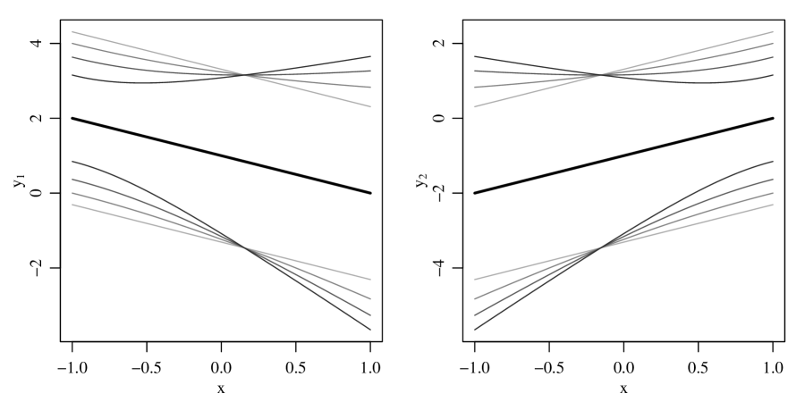
Figure 2: Population mean and variance functions for the simulation study. The black line is the mean function, and the gray lines give the mean plus and minus two standard deviations under $w\in\{0,1/3,1,3\}$.

For each combination of $n$ and $w$, 1000 datasets were generated by simulating $x$-values from the uniform(-1,1) distribution, then simulating ${\rm y}$ conditional on $\mbox{\boldmath{${\rm x}$}}=(1,x)^{T}$ from the model given by (9). The EM-algorithm described in Section 3.1 was used to obtain parameter estimates of the model parameters. In terms of summarizing results, we first evaluate the covariance regression model in terms of its potential for improved estimation of the mean function. The first set of four columns of Table 1 compares the ratio of ${\rm E}[||\mbox{\bf{A}}-\hat{\mbox{\bf{A}}}_{\rm OLS}||^{2}]$ to ${\rm E}[||\mbox{\bf{A}}-\hat{\mbox{\bf{A}}}_{\rm CVR}||^{2}]$, the former being the MSE of the OLS estimate and the latter the MSE of the MLE from the covariance regression (CVR) model. Not surprisingly, when the sample size is low $(n=50)$ and there is little or no heteroscedasticity ($w\in\{0,1/3\}$), the OLS estimator slightly outperforms the overly complex CVR estimator. However, as the sample size increases the CVR estimator improves to roughly match the OLS estimator in terms of MSE. In the presence of more substantial heteroscedasticity ($w\in\{1,3\}$), the CVR estimator outperforms the OLS estimator for each sample size, with the MSE of the OLS estimator being around 40% higher than that of the CVR estimator for the case $w=3$.

	relative MSE				power				relative MSE
	$w$				$w$				$w$
$n$	0	1/3	1	3	0	1/3	1	3	0	1/3	1	3
50	0.92	0.93	1.01	1.36	0.083	0.106	0.550	0.993	0.98	0.98	0.98	1.36
100	0.96	0.97	1.06	1.42	0.056	0.121	0.855	1.000	1.00	1.00	1.05	1.42
200	0.99	0.99	1.06	1.41	0.057	0.154	0.996	1.000	1.00	1.00	1.06	1.41

Table 1: MSE comparison and power from the simulation study. The sample size is given by $n$ and the magnitude of the covariance effects by $w$. The first set of columns gives the ratio of the MSE of the OLS estimator to that from the covariance regression model. The second set of columns gives the estimated power of the likelihood ratio test for heteroscedasticity, and the third set of columns gives the relative MSE of the model selected estimator.

In practical data analysis settings it is often recommended to favor a simple model over a more complex alternative unless there is substantial evidence that the simple model fits poorly. With this in mind, we consider the following estimator $\hat{\mbox{\bf{A}}}_{\rm MS}$ based on model selection:

1. Perform the level-$\alpha$ likelihood ratio test of ${\rm H}_{0}:\mbox{\bf{B}}=\mbox{\bf{0}}$ versus ${\rm H}_{1}:\mbox{\bf{B}}\neq\mbox{\bf{0}}$

2. Calculate $\hat{\mbox{\bf{A}}}_{\rm MS}$ as follows:

   1. If ${\rm H}_{0}$ is rejected, set $\hat{\mbox{\bf{A}}}_{\rm MS}=\hat{\mbox{\bf{A}}}_{\rm CVR}$;

   2. If ${\rm H}_{0}$ is accepted, set $\hat{\mbox{\bf{A}}}_{\rm MS}=\hat{\mbox{\bf{A}}}_{\rm OLS}$.

The asymptotic null distribution of the -2 log-likelihood ratio statistic is a $\chi^{2}$ distribution with $p\times q$ degrees of freedom. The second set of four columns in Table 1 describes the estimated finite-sample level and power of this test when $\alpha=0.05$. The level of the test can be obtained from the first column of the set, as $w=0$ corresponds to the null hypothesis being true. The level is somewhat liberal when $n=50$, but is closer to the nominal level for the larger sample sizes (note that power estimates here are subject to Monte Carlo error, and that 95% Wald intervals for the actual levels contain 0.05 for both $n=100$ and $n=200$). As expected, the power of the test increases as either the sample size or the amount of heteroscedasticity increase. The MSE of $\hat{\mbox{\bf{A}}}_{\rm OLS}$ relative to $\hat{\mbox{\bf{A}}}_{\rm MS}$, given in the third set of four columns, shows that the model selected estimate $\hat{\mbox{\bf{A}}}_{\rm MS}$ performs quite well, having essentially the same MSE as the OLS estimate when there is little or no heteroscedasticity, but having the same MSE as the CVR estimate in the presence of more substantial heteroscedasticity.

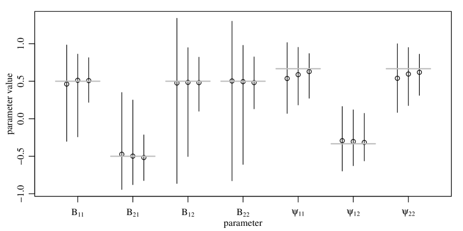
Figure 3: Sampling distribution quantiles of the covariance regression parameter estimates for the case $w=1$ and $n\in\{50,100,200\}$. Horizontal gray lines are the true parameter values, and vertical lines and dots give the 2.5, 50 and 97.5 percentiles of the sampling distributions for each parameter and sample size, with sample size increasing from left to right for each group of three lines.

$n$	$b_{1,1}$	$b_{1,2}$	$b_{2,1}$	$b_{2,2}$	$\psi_{1,1}$	$\psi_{1,2}$	$\psi_{2,2}$
50	0.89	0.88	0.90	0.89	0.88	0.94	0.87
100	0.92	0.92	0.93	0.93	0.93	0.96	0.93
200	0.94	0.95	0.94	0.93	0.95	0.97	0.96

Table 2: Observed coverage of $95\%$ Wald confidence intervals, for the case $w=1$.

Beyond improved estimation of the regression matrix ${\rm A}$, the covariance regression model can be used to describe patterns of non-constant covariance in the data. If the likelihood ratio test described above rejects the constant covariance model, it will often be of interest to obtain point estimates and confidence intervals for B and ${\rm\Psi}$. In terms of point estimates, recall that the sign of B is not identifiable, with B and $-\mbox{\bf{B}}$ corresponding to the same covariance function. To facilitate a description of the simulation results, estimates of B were processed as follows: Given a parameter value $\check{\mbox{\bf{B}}}$ from the EM algorithm, the value of $\hat{\mbox{\bf{B}}}$ was taken to be either $\check{\mbox{\bf{B}}}$ or $-\check{\mbox{\bf{B}}}$ depending on which was closer to $\mbox{\bf{B}}=[(1,-1)^{T}(1,1)^{T}]$.

In the interest of brevity we present detailed results only for the case $w=1$, as results for other values of $w$ follow similar patterns. Figure 3 shows 2.5%, 50% and 97.5% quantiles of the empirical distribution of the 1000 $\hat{\mbox{\bf{B}}}$ and $\hat{{\mbox{\boldmath{${\rm\Psi}$}}}}$-values for the case $w=1$. Although skewed, the sampling distributions of the point estimates are generally centered around their correct values, becoming more concentrated around the truth as the sample size increases. The skew of the sampling distributions diminishes as the log-likelihood becomes more quadratic with increasing sample size.

Regarding confidence intervals, as described in Section 3.3, an asymptotic approximation to the variance-covariance matrix of $\hat{\mbox{\boldmath{${\rm B}$}}}$ and $\hat{{\mbox{\boldmath{${\rm\Psi}$}}}}$ can be obtained by plugging the values of the MLEs into the inverse of the expected information matrix. Approximate confidence intervals for individual parameters can then be constructed with Wald intervals. For example, an approximate 95% confidence interval for $b_{j,k}$ would be $\hat{b}_{j,k}\pm 1.96\times{\rm se}(\hat{b}_{j,k})$, where the standard error ${\rm se}(\hat{b}_{j,k})$ is the approximation of the standard deviation of $\hat{b}_{j,k}$ based on the expected information matrix. Table 2 presents empirical coverage probabilities from the simulation study for the case $w=1$ (results for other non-zero values of $w$ are similar). The intervals are generally a bit too narrow for the low sample size case $n=50$, although the coverage rates become closer to the nominal level as the sample size increases.

4.1 Multiple regressors

The proposed covariance regression model may be of particular use when the covariance depends on several explanatory variables but in a simple way. For example, consider the case of one continuous regressor $x_{1}$ and two binary regressors $x_{2}$ and $x_{3}$. There are four covariance functions of $x_{1}$ in this case, one for each combination of $x_{2}$ and $x_{3}$. As in the case of mean regression, a useful parsimonious model might assume that the differences between the groups can be parameterized in a relatively simple manner. For example, consider the random effects representation of a covariance regression model with additive effects:

$$\mbox{\boldmath{${\rm y}$}}_{i} = \mbox{\bf{A}}\mbox{\boldmath{${\rm x}$}}_{i}+\gamma_{i}\times\mbox{\bf{B}}\mbox{\boldmath{${\rm x}$}}_{i}+\mbox{\boldmath{${\rm\epsilon}$}}_{i}$$

$$\mbox{\bf{B}}\mbox{\boldmath{${\rm x}$}}_{i} = \mbox{\boldmath{${\rm b}$}}_{0}+\mbox{\boldmath{${\rm b}$}}_{1}x_{i,1}+\mbox{\boldmath{${\rm b}$}}_{2}x_{i,2}+\mbox{\boldmath{${\rm b}$}}_{3}x_{i,3},$$

so $\mbox{\boldmath{${\rm b}$}}_{0},\mbox{\boldmath{${\rm b}$}}_{1},\mbox{\boldmath{${\rm b}$}}_{2},\mbox{\boldmath{${\rm b}$}}_{3}$ are four $p\times 1$ column vectors of ${\rm B}$. In particular, suppose $\mbox{\bf{A}}\mbox{\boldmath{${\rm x}$}}_{i}=(1,-1)^{T}+(-1,1)^{T}x_{i,1}$, ${\rm Cov}[\mbox{\boldmath{${\rm\epsilon}$}}_{i}]=\mbox{\boldmath{${\rm\Psi}$}}_{0}/(w+1)$ where $\mbox{\boldmath{${\rm\Psi}$}}_{0}$ is as in the first simulation study and

$$\mbox{\bf{B}}=\frac{w}{w+1}\left(\begin{array}[]{rrrr}1&1&1/2&1\\ -1&1&-1/2&-1\end{array}\right).$$

Note that the “baseline” case of $x_{2}=x_{3}=0$ corresponds to the covariance function in the previous simulation study, and the effects of non-zero values of $x_{2}$ or $x_{3}$ are additive on the scale of the random effect $\gamma_{i}$. The four covariance functions of $x_{1}$ are plotted in Figure 4 for the case $w=1/3$.

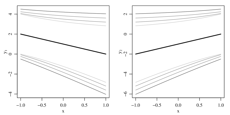
Figure 4: Population mean and variance functions for the second simulation study. The black line is the mean function, and the gray lines give the mean plus and minus two standard deviations under $w=1/3$. Moving out from the center, the gray lines correspond to $(x_{2},x_{3})=(0,0)$, $(1,0)$, $(0,1)$ and $(1,1)$.

As in the previous study, we generated 1000 datasets for each value of $w\in\{1/3,1,3\}$ with a sample size of $n=50$ for each of the four groups. We estimated the parameters in the covariance regression model as before using the EM algorithm, and compared the results to those obtained using the kernel estimator described in Yin et al. (2010). This latter approach requires a user-specified kernel bandwidth, which we obtain by cross-validation separately for each simulated dataset.

We compare each estimated covariance function $\hat{\mbox{\boldmath{${\rm\Sigma}$}}}_{\rm x}$ to the truth ${\mbox{\boldmath{${\rm\Sigma}$}}}_{\rm x}$ with a discrepancy function given by

$$g(\hat{\mbox{\boldmath{${\rm\Sigma}$}}}_{\rm x}:{\mbox{\boldmath{${\rm\Sigma}$}}}_{\rm x})=\sum_{x_{1}\in\mathcal{X}}\sum_{x_{2}=0}^{1}\sum_{x_{3}=0}^{1}\left(\log|\hat{\mbox{\boldmath{${\rm\Sigma}$}}}_{\rm x}|+{\rm tr}(\hat{\mbox{\boldmath{${\rm\Sigma}$}}}^{-1}_{\rm x}{\mbox{\boldmath{${\rm\Sigma}$}}}_{\rm x})\right),$$

where $\mathcal{X}$ is a set of 10 equally-spaced $x_{1}$-values between -1 and 1. Note that this discrepancy is minimized by the true covariance function. For the case $w=1/3$ where the heteroscedasticity is a minimum, the CVR estimator had a lower value of the function $g$ than the kernel density estimator in 73.2% of the simulations. For the $w=1$ and $w=3$ cases, the CVR estimator had a lower $g$-value in 98.5% and 99.5% of the simulations, respectively, with the average difference in $g$ between the two estimators increasing with increasing $w$. However, the point here is not that the kernel estimator is deficient. Rather, the point is that the kernel estimator cannot take advantage of situations in which the covariance functions across groups are similar in some easily parameterizable way.

5 Higher rank models

The model given by Equation 1 restricts the difference between $\mbox{\boldmath{${\rm\Sigma}$}}_{\rm x}$ and the baseline matrix ${\rm\Psi}$ to be a rank-one matrix. To allow for higher-rank deviations, consider the following extension of the random-effects representation given by Equation 4:

$$\mbox{\bf{y}}=\mbox{\boldmath{${\rm\mu}$}}_{\rm x}+\gamma\times\mbox{\bf{B}}\mbox{\bf{x}}+\phi\times\mbox{\bf{C}}\mbox{\bf{x}}+\mbox{\boldmath{${\rm\epsilon}$}},$$ (10)

where $\gamma$ and $\phi$ are mean-zero variance-one random variables, uncorrelated with each other and with ${\rm\epsilon}$. Under this model, the covariance of ${\rm y}$ is given by

$$\mbox{\boldmath{${\rm\Sigma}$}}_{\rm x}={\mbox{\boldmath{${\rm\Psi}$}}}+\mbox{\bf{B}}\mbox{\bf{x}}\mbox{\bf{x}}^{T}\mbox{\bf{B}}^{T}+\mbox{\bf{C}}\mbox{\bf{x}}\mbox{\bf{x}}^{T}\mbox{\bf{C}}^{T}.$$

This model allows the deviation of $\mbox{\boldmath{${\rm\Sigma}$}}_{\rm x}$ from the baseline ${\rm\Psi}$ to be of rank 2. Additionally, we can interpret the second random effect $\phi$ as allowing an additional, independent source of heteroscedasticity for the set of the $p$ response variables. Whereas the rank-1 model essentially requires that extreme residuals for one element of ${\rm y}$ co-occur with extreme residuals of the other elements, the rank-2 model allows for more flexibility, and can allow for heteroscedasticity across individual elements of ${\rm y}$ without requiring extreme residuals for all of the elements. Further flexibility can be gained by adding additional random effects, allowing the difference between $\mbox{\boldmath{${\rm\Sigma}$}}_{\rm x}$ and the baseline ${\rm\Psi}$ to be of any desired rank up to and including $p$.

Identifiability:

For a rank-$r$ model with $r>1$, consider a random-effects representation given by $\mbox{\boldmath{${\rm y}$}}_{i}-\mbox{\boldmath{${\rm\mu}$}}_{{\rm x}_{i}}=\sum\gamma_{i,k}\times\mbox{\bf{B}}^{(k)}\mbox{\boldmath{${\rm x}$}}_{i}+\mbox{\boldmath{${\rm\epsilon}$}}_{i}$. Let $\mbox{\bf{B}}_{1}=(\mbox{\bf{b}}_{1}^{(1)},\ldots,\mbox{\bf{b}}_{1}^{(r)})$ be the $p\times r$ matrix defined by the first columns of $\mbox{\bf{B}}^{(1)},\ldots,\mbox{\bf{B}}^{(r)}$, and define $\{\mbox{\bf{B}}_{j}:k=1,\ldots,q\}$ similarly. The model can then be expressed as

$$\mbox{\boldmath{${\rm y}$}}_{i}-\mbox{\boldmath{${\rm\mu}$}}_{{\rm x}_{i}}=\sum_{k=1}^{q}x_{k}\mbox{\bf{B}}_{k}\mbox{\boldmath{${\rm\gamma}$}}_{i}+\mbox{\boldmath{${\rm\epsilon}$}}_{i}.$$

Now suppose that $\mbox{\boldmath{${\rm\gamma}$}}_{i}$ is allowed to have a covariance matrix ${\rm\Phi}$ not necessarily equal to the identity. The above representation shows that the model given by $\{\mbox{\bf{B}}_{1},\ldots,\mbox{\bf{B}}_{k},\mbox{\boldmath{${\rm\Phi}$}}\}$ is equivalent to the one given by $\{\mbox{\bf{B}}_{1}\mbox{\boldmath{${\rm\Phi}$}}^{1/2},\ldots,\mbox{\bf{B}}_{k}\mbox{\boldmath{${\rm\Phi}$}}^{1/2},\mbox{\bf{I}}\}$, and so without loss of generality it can be assumed that $\mbox{\boldmath{${\rm\Phi}$}}=\mbox{\bf{I}}$, i.e. the random effects are independent with unit variance. In this case, note that ${\rm Var}[\mbox{\boldmath{${\rm\gamma}$}}_{i}]={\rm Var}[\mbox{\bf{H}}\mbox{\boldmath{${\rm\gamma}$}}_{i}]$ where ${\rm H}$ is any $r\times r$ orthonormal matrix. This implies that the covariance function $\mbox{\boldmath{${\rm\Sigma}$}}_{\rm x}$ given by $\{\mbox{\bf{B}}_{1},\ldots,\mbox{\bf{B}}_{k},\mbox{\bf{I}}\}$ is equal to the one given by $\{\mbox{\bf{B}}_{1}\mbox{\bf{H}},\ldots,\mbox{\bf{B}}_{k}\mbox{\bf{H}},\mbox{\bf{I}}\}$ for any orthonormal H, and so the parameters in the higher rank model are not completely identifiable. One possible identifiability constraint is to restrict $\mbox{\bf{B}}_{1}=\{\mbox{\boldmath{${\rm b}$}}_{1}^{(1)},\ldots,\mbox{\boldmath{${\rm b}$}}_{1}^{(r)}\}$, the matrix of first columns of $\mbox{\bf{B}}^{(1)},\ldots,\mbox{\bf{B}}^{(r)}$, to have orthogonal columns.

Estimation:

The random-effects representation for a rank-$r$ covariance regression model is given by

$$\mbox{\boldmath{${\rm y}$}}_{i} = \mbox{\boldmath{${\rm\mu}$}}_{{\rm x}_{i}}+\sum_{k=1}^{r}\gamma_{i,k}\times\mbox{\bf{B}}^{(k)}\mbox{\boldmath{${\rm x}$}}_{i}+\mbox{\boldmath{${\rm\epsilon}$}}_{i}$$

$$= \mbox{\boldmath{${\rm\mu}$}}_{{\rm x}_{i}}+\tilde{\mbox{\bf{B}}}(\mbox{\boldmath{${\rm\gamma}$}}_{i}\otimes\mbox{\boldmath{${\rm x}$}}_{i})+\mbox{\boldmath{${\rm\epsilon}$}}_{i}\ ,\ \mbox{where}\ \tilde{\mbox{\bf{B}}}=(\mbox{\bf{B}}^{(1)},\ldots,\mbox{\bf{B}}^{(r)}).$$

Estimation for this model can proceed with a small modification of the Gibbs sampling algorithm given in Section 3, in which $\mbox{\bf{B}}^{(k)}$ and $\{\gamma_{i,k},i=1,\ldots,n\}$ are updated for each $k\in\{1,\ldots,r\}$ separately. An EM-algorithm is also available for estimation of this general rank model. The main modification to the algorithm presented in Section 3.1 is that the conditional distribution of each $\mbox{\boldmath{${\rm\gamma}$}}_{i}$ is a multivariate normal distribution, which leads to a more complex E-step in the procedure, while the M-step is equivalent to a multivariate least squares regression estimation, as before. We note that, in our experience, convergence of the EM-algorithm for ranks greater than 1 can be slow, due to the identifiability issue described above.

6 Example: Lung function and height data

To illustrate the use of the covariance regression model we analyze data on forced expiratory volume (FEV) in liters and height in inches of 654 Boston youths (Rosner, 2000). One feature of these data is the general increase in the variance of these variables with age, as shown in Figure 5.

Figure 5: FEV and height data, as a function of age. The lines correspond to the mean functions plus and minus two standard deviations, as estimated by rank 1 and rank 2 covariance regression models, in gray and black respectively.

As the mean responses for these two variables are also increasing with age, one possible modeling strategy is to apply a variance stabilizing transformation to the data. In general, such transformations presume a particular mean-variance relationship, and choosing an appropriate transformation can be prone to much subjectivity. As an alternative, a covariance regression model allows heteroscedasticity to be modeled separately from mean function, and also allows for modeling on the original scale of the data.

6.1 Maximum likelihood estimation

Ages for the 654 subjects ranged from 3 to 19 years, although there were only two 3-year-olds and three 19-year-olds. We combine the data from children of ages 3 and 19 with those of the 4 and 18-year-olds, respectively, giving a sample size of at least 8 in each age category.

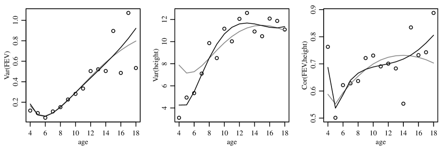
Figure 6: Sample variances and correlations as a function of age, along with rank 1 and 2 covariance regression fits in gray and black lines, respectively.

As seen in Figure 5, average FEV and height are somewhat nonlinear in age. We model the mean functions of FEV and height as cubic splines with knots at ages 4, 11 and 18, so that that ${\rm E}[\mbox{\boldmath{${\rm y}$}}_{i}|{\rm age}_{i}]=\mbox{\bf{A}}\mbox{\boldmath{${\rm w}$}}_{i}$, where $\mbox{\boldmath{${\rm y}$}}_{i}^{T}=({\rm FEV}_{i},{\rm height}_{i})$ and $\mbox{\boldmath{${\rm w}$}}_{i}$ is a vector of length 5 determined by ${\rm age}_{i}$ and the spline basis. For the regressor in the variance function we use $\mbox{\boldmath{${\rm x}$}}_{i}=(1,{\rm age}_{i}^{1/2},{\rm age}_{i})^{T}$. Note that including ${\rm age}^{1/2}$ as a regressor results in linear age terms being in the model. We also fit both rank 1 and rank 2 models to these data, and compare their relative fit:

Rank 1 model: ${\rm Cov}[\mbox{\boldmath{${\rm y}$}}_{i}|{\rm age}_{i}]=\mbox{\boldmath{${\rm\Psi}$}}+\mbox{\bf{B}}\mbox{\boldmath{${\rm x}$}}_{i}\mbox{\boldmath{${\rm x}$}}_{i}^{T}\mbox{\boldmath{${\rm B}$}}^{T}$

Rank 2 model: ${\rm Cov}[\mbox{\boldmath{${\rm y}$}}_{i}|{\rm age}_{i}]=\mbox{\boldmath{${\rm\Psi}$}}+\mbox{\bf{B}}\mbox{\boldmath{${\rm x}$}}_{i}\mbox{\boldmath{${\rm x}$}}_{i}^{T}\mbox{\boldmath{${\rm B}$}}^{T}+\mbox{\boldmath{${\rm C}$}}\mbox{\boldmath{${\rm x}$}}_{i}\mbox{\boldmath{${\rm x}$}}_{i}^{T}\mbox{\boldmath{${\rm C}$}}^{T}$

Parameter estimates from these two models are incorporated into Figure 5. The MLEs of the mean functions for the rank 1 and 2 models, given by thick gray and black lines respectively, are indistinguishable. There are some visible differences in the estimated variance functions, which are represented in Figure 5 by curves at the mean $\pm$ 2 times the estimated standard deviation of FEV and height as a function of age. A more detailed comparison of the estimated variance functions for the two models is given in Figure 6. The estimated variance functions for FEV match the sample variance function very well for both models, although the second plot in the figure indicates some lack of fit for the variance function for height by the rank 1 model at the younger ages.

Another means of evaluating this lack of fit is with a comparison of maximized log-likelihoods, which are -1927.809 and -1922.433 for the rank 1 and rank 2 models respectively. As discussed in Section 5 the first columns of B and C are not separately identifiable and may be transformed to be orthogonal without changing the model fit. As such, the difference in the number of parameters between the rank 1 and rank 2 models is 4. A likelihood ratio test comparing the rank 1 and rank 2 models gives a $p$-value of 0.0295, based on a $\chi^{2}_{4}$ null distribution, suggesting moderate evidence against the rank 1 model in favor of the rank 2 model.

6.2 Prediction regions

One potential application of the covariance regression model is to make prediction regions for multivariate observations. Erroneously assuming a covariance matrix to be constant in ${\rm x}$ could give a prediction region with correct coverage rates for an entire population, but incorrect rates for specific values of ${\rm x}$, and incorrect rates for populations having distributions of ${\rm x}$-values that are different from that of the data.

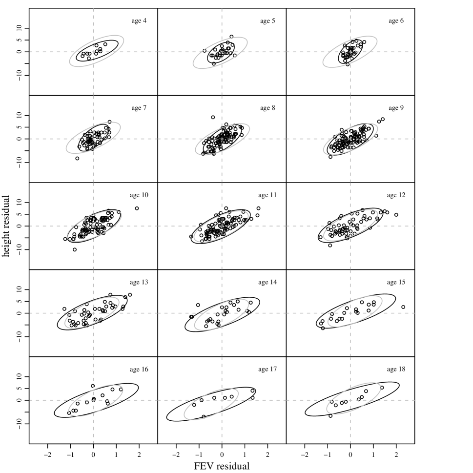
Figure 7: Observed data and approximate 90% predictive ellipsoids for each age. The black ellipsoids correspond to the covariance regression model, and the gray to the homoscedastic multivariate normal model.

For the FEV data, an approximate 90% prediction ellipse for ${\rm y}$ for each age can be obtained from the set

$$\{\mbox{\boldmath{${\rm y}$}}:(\mbox{\boldmath{${\rm y}$}}-\hat{\mbox{\boldmath{${\rm\mu}$}}}_{\rm age})^{T}\hat{\mbox{\boldmath{${\rm\Sigma}$}}}_{\rm age}^{-1}(\mbox{\boldmath{${\rm y}$}}-\hat{\mbox{\boldmath{${\rm\mu}$}}}_{\rm age})<\chi^{2}_{.9,2}\},$$

where $\hat{\mbox{\boldmath{${\rm\mu}$}}}_{\rm age}=\hat{\mbox{\bf{A}}}\mbox{\boldmath{${\rm w}$}}$, $\hat{\mbox{\boldmath{${\rm\Sigma}$}}}_{\rm age}=\hat{{\mbox{\boldmath{${\rm\Psi}$}}}}+\hat{\mbox{\bf{B}}}\mbox{\boldmath{${\rm x}$}}\mbox{\boldmath{${\rm x}$}}^{T}\hat{\mbox{\bf{B}}}^{T}$ and ${\rm w}$ and ${\rm x}$ are vector-valued functions of age as described above.

Ellipses corresponding to the fit from the rank 2 model are displayed graphically in Figure 7, along with the data and an analogous predictive ellipse obtained from the homoscedastic model.

age group
	4	5	6	7	8	9	10	11	12	13	14	15	16	17	18
sample size	11	28	37	54	85	94	81	90	57	43	25	19	13	8	9
homoscedastic	1	.96	.97	.96	.96	.95	.95	.88	.75	.81	.76	.74	.92	.75	.78
heteroscedastic	1	.86	.92	.89	.88	.93	.95	.91	.89	.91	.88	.89	.92	.88	.89

Table 3: Age-specific coverage rates for the 90% homoscedastic predictive ellipse and the 90% heteroscedastic (covariance regression) predictive ellipse.

Averaged across observations from all age groups, the homo- and heteroscedastic ellipses contain 90.1% and 90.8% of the observed data respectively, both percentages being very close to the nominal coverage rate of 90%. However, as can be seen from Table 3, the homoscedastic ellipse generally overcovers the observed data for the younger age groups, and undercovers for the older groups. In contrast, the flexibility of the covariance regression model allows the confidence ellipsoids to change size and shape as a function of age, and thus match the nominal coverage rate fairly closely across the different ages.

7 Discussion

This article has presented a model for a covariance matrix ${\rm Cov}[\mbox{\boldmath{${\rm y}$}}|\mbox{\boldmath{${\rm x}$}}]=\mbox{\boldmath{${\rm\Sigma}$}}_{\rm x}$ as a function of an explanatory variable ${\rm x}$. We have presented a geometric interpretation in terms of curves along the boundary of a translated positive definite cone, and have provided a random-effects representation that facilitates parameter estimation. This covariance regression model goes beyond what can be provided by variance stabilizing transformations, which serve to reduce the relationship between the mean and the variance. Unlike models or methods which accommodate heteroscedasticity in the form of a mean-variance relationship, the covariance regression model allows for the mean function $\mbox{\boldmath{${\rm\mu}$}}_{\rm x}$ to be separately parameterized from the variance function $\mbox{\boldmath{${\rm\Sigma}$}}_{\rm x}$.

The covariance regression model accommodates explanatory variables of all types, including categorical variables. This could be useful in the analysis of multivariate data sampled from a large number of groups, such as groups defined by the cross-classification of several categorical variables. For example, it may be desirable to estimate a separate covariance matrix for each combination of age group, education level, race and religion in a given population. The number of observations for each combination of explanatory variables may be quite small, making it impractical to estimate a separate covariance matrix for each group. One strategy, taken by Flury (1984) and Pourahmadi et al. (2007), is to assume that a particular feature of the covariance matrices (principal components, correlation matrix, Cholesky decomposition) is common across groups. A simple alternative to assuming that certain features are exactly preserved across groups would be a covariance regression model, allowing a parsimonious but flexible representation of the heteroscedasticity across the groups.

While neither the covariance regression model nor its random effects representation in Section 2 assume normally distributed errors, normality was assumed for parameter estimation in Section 3. However, accommodating other types of error distributions is feasible and straightforward to implement in some cases. For example, heavy-tailed error distributions can be accommodated with a multivariate $t$ model, in which the error term can be written as a multivariate normal random variable multiplied by a $\chi^{2}$ random variable. Estimates based upon this data-augmented representation can then be made using the EM algorithm or the Gibbs sampler (see, for example, Gelman et al. (2004, Chapter 17)).

Like mean regression, a challenge for covariance regression modeling is variable selection, i.e. the choice of an appropriate set of explanatory variables. One possibility is to use selection criteria such as AIC or BIC, although non-identifiability of some parameters in the higher-rank models requires a careful accounting of the dimension of the model. Another possibility may be to use Bayesian procedures, either by MCMC approximations to Bayes factors, or by explicitly formulating a prior distribution to allow some coefficients to be zero with non-zero probability.

Replication code and data for the analyses in this article are available at the first author’s website: www.stat.washington.edu/~hoff

References

- Box and Cox (1964) Box, G. E. P. and D. R. Cox (1964). An analysis of transformations. (With discussion). J. Roy. Statist. Soc. Ser. B 26, 211–252.
- Carroll (1982) Carroll, R. J. (1982). Adapting for heteroscedasticity in linear models. Ann. Statist. 10(4), 1224–1233.
- Carroll et al. (1982) Carroll, R. J., D. Ruppert, and R. N. Holt, Jr. (1982). Some aspects of estimation in heteroscedastic linear models. In Statistical decision theory and related topics, III, Vol. 1 (West Lafayette, Ind., 1981), pp. 231–241. New York: Academic Press.
- Chiu et al. (1996) Chiu, T. Y. M., T. Leonard, and K.-W. Tsui (1996). The matrix-logarithmic covariance model. J. Amer. Statist. Assoc. 91(433), 198–210.
- Engle and Kroner (1995) Engle, R. F. and K. F. Kroner (1995). Multivariate simultaneous generalized arch. Econometric Theory 11(1), 122–150.
- Flury (1984) Flury, B. N. (1984). Common principal components in groups. J. Amer. Statist. Assoc. 79(388), 892–898.
- Fong et al. (2006) Fong, P. W., W. K. Li, and H.-Z. An (2006). A simple multivariate ARCH model specified by random coefficients. Comput. Statist. Data Anal. 51(3), 1779–1802.
- Gelman et al. (2004) Gelman, A., J. B. Carlin, H. S. Stern, and D. B. Rubin (2004). Bayesian data analysis (Second ed.). Texts in Statistical Science Series. Chapman & Hall/CRC, Boca Raton, FL.
- Henderson and Searle (1979) Henderson, H. V. and S. R. Searle (1979). and operators for matrices, with some uses in Jacobians and multivariate statistics. Canad. J. Statist. 7(1), 65–81.
- Kass and Wasserman (1995) Kass, R. E. and L. Wasserman (1995). A reference Bayesian test for nested hypotheses and its relationship to the Schwarz criterion. J. Amer. Statist. Assoc. 90(431), 928–934.
- Magnus and Neudecker (1979) Magnus, J. R. and H. Neudecker (1979). The commutation matrix: some properties and applications. Ann. Statist. 7(2), 381–394.
- Mardia et al. (1979) Mardia, K. V., J. T. Kent, and J. M. Bibby (1979). Multivariate analysis. London: Academic Press [Harcourt Brace Jovanovich Publishers]. Probability and Mathematical Statistics: A Series of Monographs and Textbooks.
- McCulloch (1982) McCulloch, C. E. (1982). Symmetric matrix derivatives with applications. J. Amer. Statist. Assoc. 77(379), 679–682.
- Müller and Stadtmüller (1987) Müller, H.-G. and U. Stadtmüller (1987). Estimation of heteroscedasticity in regression analysis. Ann. Statist. 15(2), 610–625.
- Pourahmadi (1999) Pourahmadi, M. (1999). Joint mean-covariance models with applications to longitudinal data: unconstrained parameterisation. Biometrika 86(3), 677–690.
- Pourahmadi et al. (2007) Pourahmadi, M., M. J. Daniels, and T. Park (2007). Simultaneous modelling of the Cholesky decomposition of several covariance matrices. Journal of Multivariate Analysis 98(3), 568–587.
- Rosner (2000) Rosner, B. (2000). Fundamentals of Biostatistics. Duxbury Press.
- Rutemiller and Bowers (1968) Rutemiller, H. C. and D. A. Bowers (1968). Estimation in a heteroscedastic regression model. J. Amer. Statist. Assoc. 63, 552–557.
- Scott and Handcock (2001) Scott, M. and M. Handcock (2001). Covariance Models for Latent Structure in Longitudinal Data. Sociological Methodology, 265–303.
- Smyth (1989) Smyth, G. K. (1989). Generalized linear models with varying dispersion. J. Roy. Statist. Soc. Ser. B 51(1), 47–60.
- Yin et al. (2010) Yin, J., Z. Geng, R. Li, and H. Wang (2010). Nonparametric covariance model. Statist. Sinica 20(1), 469–479.
- Zellner (1986) Zellner, A. (1986). On assessing prior distributions and Bayesian regression analysis with -prior distributions. In Bayesian inference and decision techniques, Volume 6 of Stud. Bayesian Econometrics Statist., pp. 233–243. Amsterdam: North-Holland.