We develop the classical and quantum theory of a spinning particle moving in a Möbius strip. We first propose a Lagrangian for such a system and then we proceed to quantize the system via the constraint Hamiltonian system formalism. Our results may be of particular interest in several physical scenarios, including solid state physics and optics. In fact, the present work may shed some new light on the recent discoveries on condensed matter concerning topological insulators.

Keywords: Möbius strip, constrain Hamiltonian systems, topological insulators.

PACS: 03.65.Ca; 11.10.Ef; 73.25.+i; 73.40.-c

February, 2011

1. Introduction

Recent discoveries on condensed matter physics have opened new ways on topology and physics. In particular, this is evident in the new state of matter known as topological insulators which behaves as insulators in the bulk but have topological stable electronic states at its border; giving rise to a conductor state [1-2]. The explanation of this phenomenon resides on the type of electronic states that are present at the border: they are topologically different to those states in the bulk.

A way to interpret this condition of matter has been proposed as the case of a cylinder and a Möbius strip [3]. Both surfaces can be obtained from the gluing the two extremes of a rectangle band: one directly but the other after a half twist. In such a case, it is impossible to transform one into the other. In fact, the Möbius strip of the latter example cannot be modified in any way onto the cylinder of the former. As Zhang [4] has remarked this phenomena is the kind of difference between the electronic states in the topological insulator. The electronic states in the bulk have an energy gap at the Fermi level but at the border, the electronic states lay within the gap giving the material its metallic properties.

The existence of this type of behavior was predicted in 2006 for bi-dimensional systems with band structure in which quantum spin Hall effect arises from large spin orbit interaction. Zhang and his collaborators, proposed HgTe quantum dots as potential candidates and one year later, in 2007, they were reporting the first realization of these materials [5-6].

Subsequent studies [7-8] have found materials such as the $Bi_{2}Te_{3}$, in which a three-dimensional topological insulator state has been observed. Moreover, following the Möbius - cylinder parallelism, some researchers have studied graphene type structures with one half twist, two and several more twist, observing whether they present the kind of edge states which we mentioned above. Two years ago, in 2009, Z. L. Guo et al. published a Physical Review B paper in which they analyze the edge states in a Möbius graphene strip [9]. In fact, they describe a current through a Möbius ring. Moreover, last year, Wang and colaborators, made some ab initio studies for Möbius graphene strips with fixed length but changing its width [10]. They observed the edge states with non zero magnetic moment, confirming the topological insulator behavior.

Even more recently Chih-Wei Chang et al. [11] have discovered that electromagnetic Möbius symmetry can be successfully introduced into composite metamolecular systems made from metals and dielectrics. This discovery opens the door for exploiting novel phenomena in metamaterials.

In all these studies the starting point is the Schrödinger equation with appropriate boundary conditions. However, the results of this studies depend very much on the model involved. This has to do with the lack of a systematic way to consider the Möbius strip at the classical and quantum levels. Motivated by these observations in this work we develop the classical and quantum theory of a spinning object moving in a Möbius strip. We first propose a Lagrangian for such a system and then we proceed to quantize the system via the Dirac’s constraint Hamiltonian system formalism [12]-[13] (in particular see Ref. [14] and references therein). We prove that this Lagrangian-Hamiltonian Möbius strip mechanism can be used in general and not only in any particular case.

The paper is organized as follows. In the section 2, we briefly describe the topology of Möbius strip and discuss some of its special properties. In section 3, we present a brief description of the Hamiltonian constraint method. In section 4, we discuss the quantization of the classical motion of a spinning particle in the Möbius strip. In last section, we discus some of the characteristics of those states and extract some conclusions.

2. Möbius Strip

The Möbius strip [15-16] is a bi-dimensional manifold with only one face, and can be built from a strip of paper as follows: took the band and join together its both ends but being sure to twist one of them a half turn as it is shown in Figure 1. It is possible to confirm that the Möbius strip has one side and a single border.

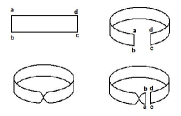
Figure 1: How to build a Möbius strip

We observe that the vector $\hat{n}$, perpendicular to the plane at any point $\bar{p}$ on the Möbius strip, will change its direction as we move along the centre line(meridian) of the strip; this normal vector will be $-\hat{n}$ when we return to the $\bar{p}\$point. This means that our strip cannot be oriented in space and for this reason we say that the Möbius strip is a non-oriented surface.

Indeed, the presence of a Möbius strip can used to define the concept of oriented surface; any surface containing a band topologically equal to a Möbius strip it is a non-oriented manifold [15]. Another way to say this, is that a surface is oriented if it has two sides.

A straight forward result that can be reached from the definition of this interesting strip, is that the normal vector $\hat{n}\$at the meridian requires to go through the circle twice in order to return to its original orientation; such a behavior is similar to that of the spin in the Stern-Gerlach experiments discussed by Feynmann [17].

If we want to analyses the movement of a spinning particle moving along a Möbius strip, we need to consider some relevant facts on this non-oriented surface. First of all, we look at the parametric representation of this surface:

$$\begin{array}[]{c}x=R\sin u+v\sin{\frac{u}{2}}\sin u,\\ \\ y=R\cos u+v\sin{\frac{u}{2}}\cos u,\\ \\ z=v\cos{\frac{u}{2},}\end{array}$$ (1)

where $u\in[0,2\pi)\$ and $v\in[-1/3,+1/3]$. As we can see, if the particle is moving along de meridian line i.e. when $v=0$; it describes a circle of radius $R$ in the plane $xy$. However, as the particle moves around this circle, the vector normal to the surface turns in such a way that it needs two complete turns to recover its original orientation. This effect can be seen when one translate the normal vector $\hat{n}$ along the meridian.

Consider the directional derivatives $e_{(A)}^{i}=\frac{\partial x^{i}}{\partial\xi^{A}}$, with $\xi^{A}=(u,v)$. Using (1) we get

$$\begin{array}[]{l}e_{1}^{1}=\frac{\partial x}{\partial u}=R\cos u+v\left(\frac{1}{2}\cos{\frac{u}{2}}\sin u+\sin{\frac{u}{2}}\cos u\right),\\ \\ e_{1}^{2}=\frac{\partial y}{\partial u}=-R\sin u+v\left(\frac{1}{2}\cos{\frac{u}{2}}\cos u-\sin{\frac{u}{2}}\sin u\right),\\ \\ e_{1}^{3}=\frac{\partial z}{\partial u}=-\frac{1}{2}v\sin{\frac{u}{2},}\\ \\ e_{2}^{1}=\frac{\partial x}{\partial v}={\sin{\frac{u}{2}}\sin u,}\\ \\ e_{2}^{2}=\frac{\partial y}{\partial v}={\sin{\frac{u}{2}}\cos u,}\\ \\ e_{2}^{3}=\frac{\partial z}{\partial v}={\cos{\frac{u}{2}.}}\end{array}$$ (2)

Note that when $v=0$, from (1) one finds that the only nonvanishing components of $e_{(A)}^{i}$ are

$$\begin{array}[]{l}e_{1}^{1}=\frac{\partial x}{\partial u}=R\cos u,\\ \\ e_{1}^{2}=\frac{\partial y}{\partial u}=-R\sin u,\end{array}$$ (3)

which correspond to a circle of radius $R$ in the $xy$-plane.

The normal vector $\hat{n}$ at the centre line is given by

$$\hat{n}=\frac{\mathbf{e}_{1}\times\mathbf{e}_{2}}{e},$$

where $e\$is the determinant of $e_{(A)}^{i}$. At the centre line, we have

$$\hat{n}=-\sin u\cos{\frac{u}{2}}\hat{\imath}-\cos u\cos{\frac{u}{2}}\hat{\jmath}+\sin{\frac{u}{2}}\hat{k}.$$ (4)

Note that if $u=0$ we find $\hat{n}=-\hat{\jmath}$ and if $u=2\pi$ we get $\hat{n}=\hat{\jmath}$. While if $u=4\pi$ we obtain $\hat{n}=-\hat{\jmath}$ as expected.

3. Brief review of constraint Hamiltonian system

Let us first recall the traditional steps to quantize a classical system. One first consider the action:

$$S[q]=\int dtL(q,\frac{dq}{dt}),$$ (5)

where the Lagrangian $L$ is a function of the $q^{i}$-coordinates and the corresponding velocities $dq^{i}/dt,$ with $i=1,\dots,n$.

Defining the canonical momentum $p_{i}$ conjugate to $q^{i}$ by

$$p_{i}\equiv\frac{\partial L}{\partial(\frac{dq^{i}}{dt})},$$ (6)

it allow us to rewrites the action (1) in the form

$$S[q,p]=\int dt(\frac{dq^{i}}{dt}p_{i}-H_{c}),$$ (7)

where $H_{c}=H_{c}(q,p)$ is the canonical Hamiltonian,

$$H_{c}(q,p)\equiv\frac{dq^{i}}{dt}p_{i}-L.$$ (8)

The Poisson bracket, for arbitrary functions $f(q,p)$ and $g(q,p)$ of the canonical variables $q$ and $p$ is defined as

$$\{f,g\}=\frac{\partial f}{\partial q^{i}}\frac{\partial g}{\partial p_{i}}-\frac{\partial f}{\partial p_{i}}\frac{\partial g}{\partial q^{i}}.$$ (9)

Using (5) we find that the basic Poisson brackets are

$$\{q^{i},q^{j}\}=0,$$ (10)

$$\{p_{i},p_{j}\}=0,$$ (11)

$$\{q^{i},p_{j}\}=\delta_{j}^{i}.$$ (12)

Here, the symbol $\delta_{j}^{i}$ denotes a Kronecker delta.

The transition to quantum mechanics is made by promoting the Hamiltonian $H_{c}(q,p)$ as an operator $\hat{H}_{c}(\hat{q},\hat{p})$ via the commutators

$$[\hat{q}^{i},\hat{q}^{j}]=0,$$ (13)

$$[\hat{p}^{i},\hat{p}^{j}]=0,$$ (14)

$$[\hat{q}^{i},\hat{p}^{j}]=i\delta^{ij},$$ (15)

with $\hbar=1$. Here, $[\hat{A},\hat{B}]=\hat{A}\hat{B}-\hat{B}\hat{A}$ denotes a commutator for any arbitrary operators $\hat{A}$ and $\hat{B}$. Note that the algebra (13)-(15) is obtained from (10)-(12) via the transition $\{f,g\}\rightarrow\frac{1}{i}[\hat{f},\hat{g}]$ for two arbitrary functions $f$ and $g$ in the phase space. In addition, one assumes the quantum formula [17-18]

$$\hat{H}_{c}\mid\Psi>=i\frac{\partial}{\partial t}\mid\Psi>,$$ (16)

which determines the physical states $\mid\Psi>$ (see Refs. [12] and [13] for details).

It is worth mentioning that (16) can be obtained from a classical constraint system. In fact, let us assume that the Lagrangian $L(q,\frac{dq}{dt})$ has the form

$$L=\frac{1}{2}m_{0}(\frac{dq}{dt})^{2}-V(q).$$ (17)

In this case the action (1) becomes.

$$S[q]=\int dt(\frac{1}{2}m_{0}(\frac{dq}{dt})^{2}-V(q)).$$ (18)

If one introduces an arbitrary parameter $\tau$ such that $q^{0}\equiv t=t(\tau)$ one find that (18) can be rewritten as

$$S[q^{0},q^{i}]=\int d\tau(\frac{1}{2}m_{0}(\dot{q}^{0})^{-1}\dot{q}^{2}-\dot{q}^{0}V(q)),$$ (19)

where $\dot{A}\equiv\frac{dA}{d\tau}$ for an arbitrary variable $A$. The expression (19) suggests a possible redefininition of the Lagrangian as

$$\mathcal{L}=\frac{1}{2}m_{0}(\dot{q}^{0})^{-1}\dot{q}^{2}-\dot{q}^{0}V(q)$$ (20)

Thus, in addition to the definition of the momentum $p_{i}$ given by

$$p_{i}\equiv\frac{\partial\mathcal{L}}{\partial(\dot{q}^{i})},$$ (21)

one may also consider the momentum

$$p_{0}\equiv\frac{\partial\mathcal{L}}{\partial(\dot{q}^{0})},$$ (22)

Using (20) one sees that (21) and (22) become

$$p^{i}\equiv m_{0}(\dot{q}^{0})^{-1}\dot{q}^{i},$$ (23)

and

$$p_{0}\equiv-\frac{1}{2}m_{0}(\dot{q}^{0})^{-2}\dot{q}^{2}-V(q),$$ (24)

respectively. These two expressions can be combined to obtain the first class constraint

$$p_{0}+\frac{p^{i}p_{i}}{2m_{0}}+V(q)=0.$$ (25)

We can also show using (23) and (24) that in this case $H_{c}$ vanishes identically.

Thus, the action functional associated with $\mathcal{L}$ can be written in the phase space as

$$\mathcal{S}[q^{0},q^{i},p_{0},p_{j},\lambda^{0}]=\int d\tau(\dot{q}^{0}p_{0}+\dot{q}^{i}p_{i}-\lambda^{0}(p_{0}+\frac{p^{i}p_{i}}{2m_{0}}+V(q)),$$ (26)

where $\lambda^{0}$ is a Lagrange multipliers. Defining

$$H_{0}\equiv p_{0}+\frac{p^{i}p_{i}}{2m_{0}}+V(q),$$ (27)

we can rewrite (26) as

$$\mathcal{S}=\int d\tau(\dot{q}^{0}p_{0}+\dot{q}^{i}p_{i}-\lambda^{0}H_{0}).$$ (28)

At the quantum level we still have the algebra (13)-(15), but instead of (16) one imposes the condition

$$\hat{H}_{0}\mid\Psi>=0,$$ (29)

on the physical states $\mid\Psi>$. Observe that (29) leads to (16) if we write $\hat{p}_{0}=-i\frac{\partial}{\partial t}$ and $\hat{H}_{c}=\frac{\hat{p}^{i}\hat{p}_{i}}{2m_{0}}+V(q)$. In other words, the Schrödinger equation (16) can be derived from the constraint structure (29).

In general if in addition to $H_{0}$ one introduces additional first class constrains $H_{m}(q,p)\approx 0$, with $m=1,2...,n$, then (28) can be extended to the form

$$S[q,p]=\int_{t_{i}}^{t_{f}}d\tau(\dot{q}^{0}p_{0}+\dot{q}^{i}p_{i}-\lambda^{0}H_{0}-\lambda^{m}H_{m}),$$ (30)

and the physical states $\mid\Psi>$ must now satisfy the conditions

$$\hat{H}_{0}\mid\Psi>=0,$$ (31)

and

$$\hat{H}_{m}\mid\Psi>=0.$$ (32)

4. Spinning particle in a Möbius strip

Our spinning object model is in a sense inspired in the relativistic spherical top theory (see Ref. [13] and references therein). However, we shall focus here in the nonrelativistic case. Specifically, let us describe the motion of a non relativistic spinning object with the variables $x^{i}(\tau)$ and $e_{i}^{(a)}(\tau)$, where $\tau$ is an arbitrary parameter; $x^{i}(\tau)$ determines the position of the system, while $e_{i}^{(a)}(\tau)$ is an orthonormal frame used to determine its orientation. We also introduce the canonical conjugate variables $p_{i}$ and $\Sigma_{ij}$ associated with $x^{i}$and $e_{i}^{(a)}$ respectively. The orthonormal character of the variables $e_{i}^{(a)}$ can be expressed by

$$e_{i}^{(a)}e_{j}^{(b)}\delta_{(ab)}=\delta_{ij}.$$ (33)

Therefore the angular velocity

$$\sigma_{ij}=e_{i}^{(a)}\frac{d}{d\tau}e_{j}^{(b)}\delta_{(ab)},$$ (34)

becomes antisymmetric tensor, that is, $\sigma_{ij}=-\sigma_{ji}$. Thus, $\sigma_{ij}$ has only three rotational degrees of freedom, as it is required.

Our main assumption is that such a spinning object is confined to move along the meridian (central line) of a Möbius strip (see Figure 2).

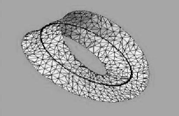
Figure 2: A Möbius strip showing its meridian cycle

Specifically, we shall consider a theory in which the motion of a spinning object is determined by the action

$$\begin{array}[]{c}S=\int d\tau[\dot{x}^{0}p_{0}+\dot{x}^{i}p_{i}+\frac{1}{2}\sigma^{ij}\Sigma_{ij}-\lambda(p_{0}+\frac{p^{i}p_{i}}{2m_{0}}+\frac{\Sigma^{ij}\Sigma_{ij}}{2m_{0}\rho^{2}}+V(x^{i}))\\ \\ -\xi(x^{i}x_{i}-r^{2})-\eta_{i}(\frac{1}{2}\varepsilon^{ijk}\Sigma_{jk}-sp^{i})-\kappa_{(a)}^{i}(e_{i}^{(a)}(\tau)-e_{i}^{(a)}(\tau+4\pi k)].\end{array}$$ (35)

Here, $\lambda,$ $\xi,$ $\eta$ and $\kappa$are Lagrange multipliers, $\rho$ is a constant describing the size of the spinning object, and finally $r^{2}$ and $s$ are considered to be constants of the motion.

Varying the parameters $\lambda,$ $\xi,$ $\eta$ and $\kappa$ we obtain the constraints

$$p_{0}+\frac{p^{i}p_{i}}{2m_{0}}+\frac{\Sigma^{ij}\Sigma_{ij}}{2m_{0}\rho^{2}}+V=0,$$ (36)

$$x^{i}x_{i}-r^{2}=0,$$ (37)

$$\varepsilon^{ijk}\Sigma_{jk}-sp^{i}=0,$$ (38)

and

$$e_{i}^{(a)}(\tau)-e_{i}^{(a)}(\tau+4\pi n)=0.$$ (39)

The first constraint determines the relation between energy $p_{0}$, kinetic energy $\frac{p^{i}p_{i}}{2m_{0}}$, rotational energy $\frac{\Sigma^{ij}\Sigma_{ij}}{2m_{0}\varrho^{2}}$ and potential energy $V$. The constraint (37) assure that the object moves on a circle. While the constraints (38) and (39) establishes the rotational motion of an orthonormal frame attached to the Möbius strip. The constraint (38) is used to force the system to have parallel angular momentum to the linear momentum during the motion along the meridian of the Möbius strip. Note that (39) specifies that the orthonormal frame needs to rotate twice in order to return to the original orientation.

Solving (38) and substituting the result into (36) gives

$$p_{0}+\frac{p^{i}p_{i}}{2m_{0}}+\frac{s^{2}p^{i}p_{i}}{2m_{0}\rho^{2}}+V=0,$$ (40)

which can be rewritten as

$$p_{0}+\frac{(1+\frac{s^{2}}{\rho^{2}})p^{i}p_{i}}{2m_{0}}+V=0.$$ (41)

Therefore, by quantizing (41) we find the Schödinger-like equation

$$\left(\hat{p}_{0}+\frac{(1+\frac{s^{2}}{\rho^{2}})\hat{p}^{i}\hat{p}_{i}}{2m_{0}}+V\right)\left|\psi\right\rangle=0,$$ (42)

which in a coordinate representation can be written as

$$\left(-i\hslash\frac{\partial}{\partial t}-\frac{\hslash^{2}(1+\frac{s^{2}}{\rho^{2}})\nabla^{2}}{2m_{0}}+V\right)\psi(t,x^{i})=0.$$ (43)

Considering that the system moves in a circle determined by the constraint (37) we get

$$\left(-i\hslash\frac{\partial}{\partial t}-\frac{\hslash^{2}}{2m_{0}^{\prime}}\frac{d^{2}}{d\theta^{2}}+V\right)\psi(t,\theta)=0,$$ (44)

where

$$m_{0}^{\prime}=\frac{m_{0}}{(1+\frac{s^{2}}{\rho^{2}})}.$$ (45)

The formula (44) is the key equation for our approach. It is important to remark that the periodicity in the orthonormal frame (39) translates at the level of the quantum equation (44) in the requirement $\psi(t,\theta)=\psi(t,\theta+4n\pi)$.

We shall now study some of the consequences of the key equation (44) in several cases. This corresponds to a number of specific forms of the potential $V$.

Example 1:

The simplest example is a free system, with $V=0$. In this case (44) is reduced to

$$\left(-i\hslash\frac{\partial}{\partial t}-\frac{\hslash^{2}}{2m_{0}^{\prime}}\frac{d^{2}}{d\theta^{2}}\right)\psi(t,\theta)=0.$$ (46)

In the stationary case (46) becomes

$$\left(-E-\frac{\hslash^{2}}{2m_{0}^{\prime}}\frac{d^{2}}{d\theta^{2}}\right)\psi(\theta)=0.$$ (47)

Thus, in this case we have the general solution

$$\psi(\theta)=\sum_{n=1}^{\infty}(a_{n}e^{\frac{in\theta p_{\theta}}{2\hslash}}-a_{n}^{\ast}e^{-\frac{in\theta p_{\theta}}{2\hslash}}),$$ (48)

where $a_{n}$ is a complex constant. Note that $\psi(\theta)=\psi(\theta+\frac{4n\pi}{p_{\theta}})$ as expected. Therefore we find that the energy eigenvalues are given by

$$E_{n}=\frac{n^{2}p_{\theta}^{2}}{8m_{0}^{\prime}}.$$ (49)

Consider a proton moving along the meridian of a Möbius strip. The root-mean square charge radius $r_{p}$ and the mass $m_{0}$ of the proton can be taken as [19-20]

$$\rho\equiv r_{p}=0.8418\times 10^{-15}m,$$ (50)

and

$$m_{0}=1.673\times 10^{-27}\quad Kg,$$ (51)

respectively. While, since the proton spin is $\Sigma=\frac{\hslash}{2}$, we can assume that the quantity $s=\frac{\Sigma}{p}$ is also of the order

$$s\sim 10^{-15}m.$$ (52)

Therefore, from (49) we find the ground state energy is or the order

$$E_{1}\sim\frac{p_{\theta}^{2}}{5.6\times 10^{-27}\quad Kg}.$$ (53)

Example 2:

As a second example let us now assume that

$$V=-\frac{e^{2}}{r}.$$ (54)

We will look for a solutions of the equation

$$\left(\frac{-\hslash^{2}\nabla^{2}}{2m_{0}^{\prime}}-\frac{e^{2}}{r}\right)\psi(x^{i})=E\psi(x^{i}).$$ (55)

Observe that (50) can be interpreted as the Schrödinger equation for the Hydrogen atom. However, one should keep in mind that we are choosing circular motion for the electron and that the wave function $\psi(x^{i})$ has periodicity $4\pi$. In fact in this case (50) can be reduced to

$$\frac{-\hslash^{2}}{2m_{0}^{\prime}}(\frac{d^{2}}{dr^{2}}+\frac{2d}{rdr}+\frac{d^{2}}{r^{2}d\theta^{2}})-\frac{e^{2}}{r})\psi(r,\theta)=E\psi(r,\theta).$$ (56)

We can propose the solution

$$\psi(r,\theta)=R(r)e^{i\frac{k\theta}{2}},$$ (57)

with eigenvalue equation

$$\hat{p}_{\theta}^{2}\psi(r,\theta)=-\hslash^{2}\frac{d^{2}}{d\theta^{2}}\psi(r,\theta)=\frac{1}{4}\hslash^{2}k^{2}\psi(r,\theta).$$ (58)

Here $k$ is considered to be an integer. Using (57) the formula (56) becomes

$$\left(\frac{-\hslash^{2}}{2m_{0}^{\prime}}(\frac{d^{2}}{dr^{2}}+\frac{2d}{rdr})+\frac{\hslash^{2}k^{2}}{8m_{0}^{\prime}r^{2}}-\frac{e^{2}}{r}\right)R(r)=ER(r).$$ (59)

Now, following standard procedure we find that the energy eigenvalues are

$$E_{n}=-\frac{1}{2}m_{0}^{\prime}c^{2}\frac{\alpha^{2}}{n^{2}},$$ (60)

where

$$\alpha=\frac{e^{2}}{\hslash c},$$ (61)

is the fine structure constant and $n$ can take the values $1,2,3,...$. But with with the restriction

$$n^{2}-n\geq\frac{k^{2}}{4},$$ (62)

instead of the usual one

$$n^{2}-n\geq l(l+1).$$ (63)

Thus, although our result (60) looks as the normal energy eigenvalues of the Hydrogen atom in fact it differs in two fundamental aspects: (1) according to (45) the constant $m_{0}^{\prime}$ depends of the size $\rho$ and the the parameter $s$ associated with the spin of the rotating object respectively, (2) the positive integer $n$ must satisfy (62) instead of (63).

Example 3:

As our final example we shall consider a constant magnetic flux $A$ through the meridian ring of the Möbius strip. In this case, one can show that (44) leads to

$$\left(-E-\frac{\hslash^{2}}{2m_{0}^{\prime}}(\frac{d}{d\theta}+A)^{2}\right)\psi(\theta)=0.$$ (64)

The eigenfunction solution of (64) can be written as

$$\psi(\theta)=e^{\frac{in\theta}{2}}.$$ (65)

This yields the energy eigenvalues

$$E_{n}=\frac{\hslash^{2}}{2m_{0}^{\prime}}(\frac{n}{4}-A)^{2},$$ (66)

where $n=0,\pm 1,\pm 2,...$. It is interesting to mention that classically the constant $A$ can be be associated with a topological term and consequently it is not observable. But (60) shows that at the quantum level $A$ changes the energy eigenvalues. However, since $A$ is related to topological structure it may be combined with the boundary conditions which in turn are related to the topology of the Möbius strip. This observation clearly motives further studies on the subject.

5. Final remarks

In this work we have derived the Schrödinger-like equation for a spinning particle moving in the meridian of a Möbius strip. The main advantage of our Lagrangian approach is that important mathematical tools of the constrains Hamiltonian theory can be used. In particular, one can determine in a systematic way the symmetries of the theory.

We show the advances of our method considering three examples; (1) $V=0$ and (2) $V=-\frac{e^{2}}{r}$, and $p\rightarrow p-A$. In the three cases the functions states have the required boundary conditions and the energy eigenvalues are quantized. In the first case the energy eigenvalues $E_{n}$ goes as as $n^{2}$. While in the second case the $E_{n}$ goes as $\frac{1}{n^{2}}$, having the form of the hydrogen atom but with the mass constant $m_{0}^{\prime}$ depending on the size $\rho$ and the internal parameter $s$ associated with the spin of the rotating object. Furthermore, the positive integer $n$ is restricted to satisfy (62) instead of (63).

It may be interesting for further research to consider the motion of spinning system in the whole Möbius strip either at the classical or quantum level. In particular, it is worth pursuing what the eigenfunctions and eigenvalues would be like for such system.

J. A. Nieto would like to thank the Departamento de Investigacion en Física for the hospitality. This work was partially supported by PROFAPI-UAS 2009.

References

- [1] S. Raghu, X.-L. Qi, C. Honerkamp, and S.-C. Zhang, Topological Mott Insulators, Phys. Rev. Lett. 100, 156401 (2008).
- [2] B. A. Bernevig, T. L. Hughes, and S.-C. Zhang, Quantum Spin Hall Effect and Topological Phase Transition in HgTe Quantum Wells, Science 314, 1757 (2006).
- [3] M. Konig, S. Wiedmann, C. Brune, A. Roth, H. Buhmann, L. W.Molenkamp, X.-L. Qi, and S. C. Zhang, Quantum Spin Hall Insulator State in HgTe Quantum Wells, Science 318, 766 (2007).
- [4] Zhang et al, Topological insulators in Bi2Se3, Bi2Te3 and Sb2Te3 with a single Dirac cone on the surface, Nature Physics, 5, 438 (2009).
- [5] M. Konig, S. Wiedmann, C. Brune, A. Roth, H. Buhmann, L. W., Molenkamp, X. L. Qi, and S.-C. Zhang, Science 318, 766 (2007).
- [6] Y. Ran Y. Zhang, A. Vishwanath, One-dimensional topologically protected modes in topological insulators with lattice dislocations, Nature Phys. 5, 298 (2009).
- [7] Y.L. Chen, et al. Experimental Realization of a Three-Dimensional Topological Insulator, Bi2Te3. Science 325, 178 (2009).
- [8] O.V. Yazyev, J.E. Moore, S.G. Louie, Spin Polarization and Transport of Surface States in the Topological Insulators Bi2Se3 and Bi2Te3 from First Principles, Phys. Rev. Lett. 105, 266806 (2010).
- [9] Z. L. Guo, Z. R. Gong, H. Dong, and C. P. Sun, Möbius graphene strip as a topological insulator, Phys. Rev. B 80, 195310, (2009).
- [10] X. Wang, X. Zheng, M. Ni, L. Zou, Z. Zenga, Theoretical investigation of Möbius strips formed from graphene, Appl. Phys. Lett. 97, 123103 (2010).
- [11] Chih-Wei Chang, Ming Liu, Sunghyun Nam, Shuang Zhang, Yongmin Liu, Guy Bartal, and Xiang Zhang, Optical Mo¨bius Symmetry in Metamaterials, Phys. Rev. Lett. 105, 235501 (2010).
- [12] M. Henneaux and C. Teitelboim, Quantization of Gauge Systems (Princeton University Press, Princeton, New Jersey, 1992).
- [13] A. Hanson, T. Regge and C. Teitelboim, Constrained Hamiltonian Systems (Accademia Nazionale dei Lincei, Roma, 1976).
- [14] V. M. Villanueva, J. A. Nieto, L. Ruiz and J. Silvas, Hamiltonian Noether theorem for gauge systems and two time physics, J. Phys. A 38, 7183 (2005); hep-th/0503093.
- [15] D.W. Blackett, Elementary Topology: A combinatorial and Algebraic Approach, (Academic Press, London, 1967).
- [16] E. D. Bloch, A First Course in Geometric Topology and Differential Geometry, (Birkhäuser, 1997).
- [17] R. Feynman, Feynman Lectures on Physics (Addison-Wesley Publishing Co., 1965).
- [18] P. A. M. Dirac, Lectures on Quantum Mechanics (New York: Yeshiva UP, 1964).
- [19] P. J. Mohr, B. N. Taylor, D. B. Newell (2007), CODATA Recommended Values of the Fundamental Physical Constants: 2006, NIST pp. 16.
- [20] R. Pohl et al., Nature 466, 213–216 (2010).