Effect of three-pion unitarity on resonance poles from heavy meson decays

Abstract

We study the final state interaction in 3$\pi$ decay of meson resonances at the Excited Baryon Analysis Center (EBAC) of JLab. We apply the dynamical coupled-channels formulation which has been extensively used by EBAC to extract N* information. The formulation satisfies the 3$\pi$ unitarity condition which has been missed in the existing works with the isobar models. We report the effect of the 3$\pi$ unitarity on the meson resonance pole positions and Dalitz plot.

1 Introduction

Why do we care the three-pion (or $\pi\pi K$, etc.) scattering system ? Some of recent and forthcoming experiments would call for serious study of the system to extract what they expect to find. One of such experiments aims to find the so-called exotic mesons in a reaction like $\pi({\rm or}\ \gamma)N\to M^{*}N\to\pi\pi\pi N$ e852 ; gluex , where $M^{*}$ is an intermediate excited meson that could be exotic. An exotic meson lies outside of the constituent quark model and speculated to be a tetraquark state or hybrid state. The spectroscopy of the hybrid states provides information about gluon self-interactions. Another experiment seeks for physics beyond the Standard Model contributing to the CP violation in B- or D-decays babar ; belle . Both of the experiments involve heavy meson decays at very short-distance followed by the formation of lighter hadrons such as pions and/or kaons. And those light hadrons are to be detected after a great number of rescatterings. Thus, for extracting what has happened at the short-distance, it is essential to understand or precisely model the final state interactions of the light hadrons.

What has conventionally been used for Dalitz plot analyses of experiments of this kind is the so-called isobar model in which it is assumed that two of the three mesons form an isobar state ($f_{0},\rho,K^{*}$, etc.), and the rest does not interact with the others (spectator). The three-body unitarity is obviously missing, and that is what we will address here. (Note that most isobar models do not take care of even two-body unitarity for the paired mesons.) Recently, the Excited Baryon Analysis Center of Jefferson Lab has extended their dynamical coupled-channels model msl , which has been extensively used to study baryon resonances, to three-meson scattering ebac . In this report, we describe our model and then apply it to the calculation of $\pi_{2}(1670)$ and $\pi_{2}(2100)$ pole positions and their 3$\pi$ decays (Dalitz plots). We will examine how significant 3$\pi$ unitarity is to extract the properties of these heavy mesons from the Dalitz plots.

2 Coupled-channels model

We consider the 3$\pi$ decay of a heavy meson ($M^{*}\to 3\pi$) and a heavy meson resonance formed in 3$\pi$ scattering ($3\pi\to M^{*}\to 3\pi$). Interesting quantities to calculate are the decay amplitude (and the corresponding Dalitz plot) for the decay, and the pole position of the resonance. In any case, we need 3$\pi$ scattering amplitudes. For calculating 3$\pi$ amplitude, first we need to develop a more basic $\pi\pi$ model. In the following, we discuss our $\pi\pi$ model and then calculation of the 3$\pi$ amplitude.

$\pi\pi$ model  For a simpler calculation, we employ an isobar-type model for $\pi\pi$ interaction so that $\pi\pi\to R\to\pi\pi\ ({\rm or}\ K\bar{K})$, where $R$ ($=f_{0},\rho$ or $f_{2}$) is an isobar. The $\pi\pi$ potentials for a partial wave (orbital angular momentum $L$, total isospin $I$) are parametrized as $\sum_{R}f^{LI}_{R,i}(p^{\prime})(W-m_{R})^{-1}f^{LI}_{R,j}(p)$, where $W$ and $m_{R}$ are the total energy and the bare mass of the isobar $R$, respectively; $f_{R,i}(p)$ is the $R\leftrightarrow i$ $(i=\pi\pi\ {\rm or}\ K\bar{K})$ vertex with $p$ being the relative momentum of $\pi\pi$ ($K\bar{K}$). The $\pi\pi$ scattering amplitude is obtained by solving the coupled-channels Lippmann-Schwinger equation with this potential.

$\pi$-isobar scattering equation  Because we have introduced the isobars ($R$), the partial wave amplitude specified by $J^{P}$ (total spin and parity) and $T$ (total isospin) can be obtained by solving the corresponding $\pi-R$ scattering equation:

$$T^{J^{P}T}_{\alpha,\beta}(p^{\prime},p;W)=V^{J^{P}T}_{\alpha,\beta}(p^{\prime},p;W)+\sum_{\gamma\gamma^{\prime}}\int^{\infty}_{0}\!\!\!q^{2}dq\ V^{J^{P}T}_{\alpha,\gamma}(p^{\prime},q;W)\ G_{\gamma\gamma^{\prime}}(q,W)T^{J^{P}T}_{\gamma^{\prime},\beta}(q,p;W)\ ,$$ (1)

where the indices $\alpha,\beta,\gamma$ specify channels ($\pi f_{0}$ or $\pi\rho$ or $\pi f_{2}$), $E_{\gamma}(q)=\sqrt{m_{\pi}^{2}+q^{2}}+\sqrt{m_{R_{\gamma}}^{2}+q^{2}}$. The $\pi-R$ Green function, $G_{\gamma\gamma^{\prime}}(q,W)$, is given by $[G^{-1}(q,W)]_{\gamma\gamma^{\prime}}=[W-E_{\gamma}(q)]\delta_{\gamma\gamma^{\prime}}-\Sigma_{\gamma\gamma^{\prime}}(q,W)$, with the self-energy ($\Sigma_{\gamma\gamma^{\prime}}$) defined as

$$\Sigma_{\gamma\gamma^{\prime}}(p,W)=\!\!\!\!\sum_{i}^{\pi\pi,K\bar{K}}\!\!\!\sqrt{m_{R_{\gamma}}m_{R_{\gamma^{\prime}}}\over E_{R_{\gamma}}(p)E_{R_{\gamma^{\prime}}}(p)}\int_{0}^{\infty}\!\!\!{E_{i}(q)\over\sqrt{E^{2}_{i}(q)+p^{2}}}{q^{2}f^{L_{\gamma}I_{\gamma}}_{R_{\gamma},i}(q)f^{L_{\gamma^{\prime}}I_{\gamma^{\prime}}}_{R_{\gamma^{\prime}},i}(q)\ dq\over W-E_{\pi}(p)-\sqrt{E^{2}_{i}(q)+p^{2}}+i\epsilon}\ .$$ (2)

The potential, $V^{J^{P}T}_{\alpha,\beta}(p^{\prime},p;W)$, includes Z-graphs [Fig. 1(a)] derived from the $\pi\pi$ model developed above. (We ignore Z-graphs with $\pi K\bar{K}$ intermediate states for simplicity.)

Figure 1: $\pi$-$R$ interaction: (a) 3$\pi$ Z-graph; (b) $M^{*}$-term

The Z-graphs, together with the self-energy [Eq. (2)], are essential to maintain the 3$\pi$ unitarity. One may also include $M^{*}$-term [Fig. 1(b)] for the $\pi$-$R$ potential.

3 Applications and results

Effect of Z-graph on pole position We examine the effect of Z-graph on the pole position of $\pi_{2}(1670)$ and $\pi_{2}(2100)$. The procedure for finding the pole position suitable for our model has been developed suzuki . A pole position is at a complex energy ($W$) for which $W-M^{0}_{M^{*}}-\Sigma_{M^{*}}(W)=0$ is satisfied; $M^{0}_{M^{*}}$ is the $M^{*}$ bare mass and $\Sigma_{M^{*}}(W)$ is the self energy of $M^{*}$ given by

$$\Sigma_{M^{*}}(W)=\sum_{\alpha,\beta}\int^{\infty}_{0}\!\!\!q^{2}dq\ \bar{g}_{M^{*},\alpha}(q)G_{\alpha\beta}(q,W)g_{M^{*},\beta}(q)\ ,$$ (3)

where $g_{M^{*},\beta}(q)$ is a $M^{*}\to\pi R$ vertex, and $\bar{g}_{M^{*},\alpha}(q)$ is a dressed vertex defined as

$$\bar{g}_{M^{*},\alpha}(p)=g_{M^{*},\alpha}(p)+\sum_{\gamma\gamma^{\prime}}\int^{\infty}_{0}\!\!\!q^{2}dq\ g_{M^{*},\gamma}(q)\ G_{\gamma\gamma^{\prime}}(W,q)\ t^{J^{P}T}_{\gamma^{\prime},\alpha}(q,p;W)\ ,$$ (4)

where $t^{J^{P}T}_{\beta,\alpha}$ is the T-matrix calculated with Eq. (1) in which the potential includes only the Z-graphs. We fit $M^{0}_{M^{*}}$ and $g_{M^{*},\alpha}$ to pole positions and branching ratios of $\pi_{2}$’s; data are taken from the Particle Data Group. Then we eliminate the Z-graphs from our model, that is, we calculate $\Sigma_{M^{*}}(W)$ with Eq. (3) in which the dressed vertex is replaced by the bare one. We find the pole positions again from $W-M^{0}_{M^{*}}-\Sigma_{M^{*}}(W)=0$. The pole for $\pi_{2}(1670)$ changes from $1672-130i$ MeV to $1689-133i$ MeV, and for $\pi_{2}(2100)$, from $2090-313i$ MeV to $2084-346i$ MeV. Thus, the Z-graphs change the pole position by $\sim$ 10% [$2\sim 3$%] for $\pi_{2}(2100)$ [$\pi_{2}(1670)$].

Effect of Z-graph on Dalitz plot We calculate the decay amplitude of a $M^{*}$ as graphically shown in Fig. 2, and then obtain the corresponding Dalitz plot.

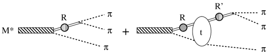
Figure 2: $M^{*}$-decay amplitude: The bulb labeled ’t’ is the T-matrix calculated with Eq. (1) in which the potential includes only the Z-graphs. The gray circle indicates the self-energy of the isobar [Eq. (2)].

In the first term of Fig. 2, two pions are paired, and the 3rd pion is the spectator. The second term includes rescatterings due to the Z-graphs. Here, we show the Dalitz plot for the $\pi_{2}(2100)$ decay in Fig. 3 (left). In order to examine the effect of the Z-graphs, we turn off the Z-graphs, i.e., we calculate only the first term in Fig. 2. We show the ratio of the Dalitz plots with and without the Z-graphs in Fig. 3 (right). In general, the Z-graphs change both the magnitude and the shape of the Dalitz plot. The effect is more significantly seen in the Dalitz plot than in the shift of the pole position.

	$\Gamma_{\rm pole}$ (MeV)	$\pi_{2}\to\pi f_{0}$ (%)	$\pi_{2}\to\pi\rho$ (%)	$\pi_{2}\to\pi f_{2}$ (%)
with Z	626	45	19	36
w/o Z	542	36	27	37

Table 1: The properties of $\pi_{2}(2100)$ extracted from models with (2nd row) and without (3rd row) the Z-graphs. The second column is the width at the pole, 3-5th columns are the branching ratios.

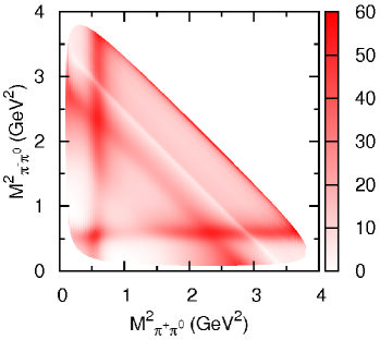
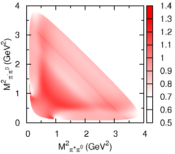
Figure 3: (left) Dalitz plot of $\pi_{2}(2100)$ decay; (right) Ratio of Dalitz plots with and w/o the Z-graphs.

We may fit to the Dalitz plot of Fig. 3 (left) with our model without the Z-graphs, by varying the $M^{*}\to\pi R$ couplings and cutoff. With a tentative error of 5% assigned to the Dalitz plot, we achieved the fit with $\chi^{2}/{\rm data}\sim 1.1$. It would be interesting to examine the properties of $M^{*}$ extracted from the two models (with or without the Z-graphs) both of which reproduce the same Dalitz plot. In Table 1, we show the width and the branching ratios of $\pi_{2}(2100)$ extracted from the two models. We find a significant difference in the properties from the two models. Although the effect of the Z-graphs depends on a system, still this results indicates an importance of including the Z-graph (3$\pi$ unitarity) in analyzing the Dalitz plot.

References

• (1) S. U. Chung et al. [E852 Collaboration], Phys. Rev. Lett. 81, 5760 (1998).
• (2) D. S. Carman [The Gluex Collaboration], AIP Conf. Proc. 814, 173 (2006).
• (3) e.g., B. Aubert et al. [BaBar Collaboration], Phys. Rev. D 78, 034023 (2008).
• (4) e.g., A. Garmash et al. [Belle Collaboration], Phys. Rev. D 71, 092003 (2005).
• (5) A. Matsuyama, T.-S. H. Lee, and T. Sato, Phys. Rept. 439, 193 (2007).
• (6) H. Kamano, T.-S. H. Lee, S. X. Nakamura, and T. Sato, in preparation.
• (7) N. Suzuki, T. Sato, and T.-S. H. Lee, Phys. Rev. C 79, 025205 (2009); ibid. 82, 045206 (2010).