Hubble Space Telescope Transmission Spectroscopy of the Exoplanet HD 189733b: High-altitude atmospheric haze in the optical and near-UV with STIS

Abstract

We present Hubble Space Telescope optical and near-ultraviolet transmission spectra of the transiting hot-Jupiter HD189733b, taken with the repaired Space Telescope Imaging Spectrograph (STIS) instrument. The resulting spectra cover the range 2900-5700 Å and reach per-exposure signal-to-noise levels greater than 11,000 within a 500 Å bandwidth. We used time series spectra obtained during two transit events to determine the wavelength dependance of the planetary radius and measure the exoplanet’s atmospheric transmission spectrum for the first time over this wavelength range. Our measurements, in conjunction with existing HST spectra, now provide a broadband transmission spectrum covering the full optical regime. The STIS data also shows unambiguous evidence of a large occulted stellar spot during one of our transit events, which we use to place constraints on the characteristics of the K dwarf’s stellar spots, estimating spot temperatures around T${}_{\mathrm{eff}}\sim$4250 K. With contemporaneous ground-based photometric monitoring of the stellar variability, we also measure the correlation between the stellar activity level and transit-measured planet-to-star radius contrast, which is in good agreement with predictions. We find a planetary transmission spectrum in good agreement with that of Rayleigh scattering from a high-altitude atmospheric haze as previously found from HST ACS camera. The high-altitude haze is now found to cover the entire optical regime and is well characterised by Rayleigh scattering. These findings suggest that haze may be a globally dominant atmospheric feature of the planet which would result in a high optical albedo at shorter optical wavelengths.

1 Introduction

Transiting planets now allow the possibility of detecting and studying extrasolar planets, from their formation and statistical properties, to the bulk composition of the planets themselves as well as their atmospheres. Atmospheric information on exoplanets can be gathered in several different ways. During a transit, an exoplanet passes in front of its host star, with some of the stellar light filtered through the planet’s atmosphere, making it possible to perform transmission spectroscopy (Charbonneau et al., 2002; Vidal-Madjar et al., 2003). Optical and infrared measurements during secondary eclipse can be used to obtain an exoplanet’s dayside emission spectra, where such properties including the temperature, thermal structure, and composition can be measured (e.g. Deming et al. 2005; Grillmair et al. 2008; Charbonneau et al. 2008; Rogers et al. 2009; Sing & López-Morales 2009). Finally, orbital phase curves can probe the global temperature distribution and study atmospheric circulation (Knutson et al., 2007a).

Transiting events around bright stars are extremely valuable, and have allowed unprecedented access to detailed atmospheric studies of extrasolar planets. Two particularly favorable cases, the hot Jupiters HD 209458b and HD 189733b, have been the focus of many followup studies and modeling efforts over the last decade. The first exoplanet atmosphere was detected by Charbonneau et al. (2002) using transits of HD 209458b with the HST STIS instrument. Sodium was later confirmed from ground-based spectrographs which measured similar absorption levels as the revised STIS data (Snellen et al., 2008; Sing et al., 2008a). HD 209458b is now known to have a very low optical albedo (Rowe et al., 2006). The overall optical transmission spectrum is consistent with H₂ Rayleigh scattering and absorption from Na, and perhaps TiO/VO (Sing et al., 2008b; Lecavelier des Etangs et al., 2008b; Désert et al., 2008).The sodium line profile also reveals the planet’s thermosphere and ionization layer at high altitudes (Vidal-Madjar et al., 2011). HD 209458b also shows evaporation of atomic H, C, O, and Si (Vidal-Madjar et al., 2003, 2004; Linsky et al., 2010) through ultraviolet observations. In the infrared, CO has been detected from high-resolution spectrographs (Snellen et al., 2010). From secondary eclipse measurements, the planet also has a well established thermal inversion layer (Knutson et al., 2008; Burrows et al., 2007).

Contrary to HD 209458b, the other well studied hot-Jupiter HD 189733b does not show spectral features in emission that would indicate a thermal inversion layer (Grillmair et al., 2008; Charbonneau et al., 2008). In addition, orbital phase curve measurements have revealed efficient redistribution via eastward jets, producing small day/night temperature contrasts (Knutson et al., 2007a, 2009). In the optical, a ground-based detection of sodium has been made from transmission spectroscopy by Redfield et al. (2008), with the wider overall optical spectrum consistent with a high altitude haze (Pont et al., 2008; Sing et al., 2009). The optical transmission spectrum of the haze is seen to become gently more transparent from blue to red wavelengths, and is consistent with Rayleigh scattering by small condensate particles, with MgSiO₃ grains suggested as a possible candidate (Lecavelier des Etangs et al., 2008a). Ultraviolet transits have also determined the planet to have an escaping atomic hydrogen atmosphere (Lecavelier Des Etangs et al., 2010). The infrared opacity is now known to include H₂O absorption, with the best current evidence coming from secondary eclipse measurements (Grillmair et al., 2008), while CO and CO₂ have also been suggested (Désert et al., 2009; Swain et al., 2009).

For highly irradiated planets, the atmosphere at optical wavelengths is vital to the energy budget of the planet, as it is where the bulk of the stellar flux is deposited. The atmospheric properties at these wavelengths are directly linked to important global properties such as atmospheric circulation, thermal inversion layers, and inflated planetary radii. Some of these features may be linked within the hot-Jupiter exoplanetary class (e.g. Fortney et al. 2008). High-S/N broadband transmission spectra of exoplanets with HST Space Telescope Imaging Spectrograph (STIS) can provide direct observational constraints and fundamental measurements of the atmospheric properties at these vital wavelengths. This is especially crucial in the near-UV and into the optical, given that JWST will not be able to observe at such wavelengths.

Here we present Hubble Space Telescope (HST) transmission spectra of HD 189733b using the STIS instrument, part of programme GO-11740 aiming to provide a reference measurement of the broadband transmission spectrum across the whole visible and near-infrared spectral range. Our observational strategy in this program is a detailed study for one exoplanet, in order to gain robust and highly constraining measurements, useful for comparative planetology. In the case of HD 189733b, this is particularly important as this planet has become a canonical hot-Jupiter along with HD 209458b, with both planets providing the foundation for what is now known about these types of exoplanets. The STIS instrument, recently repaired during the servicing mission four (SM4), has once again provided the opportunity to make extremely high S/N optical transit observations, capable of detecting and scrutinizing atmospheric constituents. In this paper, we present new HST/STIS observations, constraining the atmospheric transmission spectrum in the optical and near-UV.

2 Observations

2.1 Hubble Space Telescope STIS Spectroscopy

We observed transits of HD 189733b with the HST STIS G430L grating during 20 November 2009 and 18 May 2010 as part of program GO 11740 (P.I. FP). Similar observations to these have been made previously on the other bright hot-Jupiter exoplanet HD 209458b (Knutson et al., 2007b; Ballester, Sing & Herbert, 2007; Sing et al., 2008a). The G430L dataset consists of about 200 spectra spanning the two transit events covering the wavelength range 2,892-5,700 Å, with a resolution R of $\lambda$/$\Delta\lambda=$530–1,040 ($\sim$2 pixels; 5.5 Å), and taken with a wide 52”$\times$2” slit to minimize slit light losses. This observing technique has proven to produce high signal-to-noise (S/N) spectra which are photometrically accurate near the Poisson limit during a transit event. Both visits of HST were scheduled such that the third orbit of the spacecraft would contain the transit event, providing good coverage between second and third contact as well as an out-of-transit baseline time series before and after the transit. Exposure times of 64 seconds were used in conjunction with a 128-pixel wide sub-array, which reduces the readout time between exposures to 23 seconds, providing a 74% overall duty cycle.

The dataset was pipeline-reduced with the latest version of CALSTIS and cleaned for cosmic ray detections before performing spectral extractions. The aperture extraction was done with IRAF using a 13-pixel-wide aperture, background subtraction, and no weights applied to the aperture sum. The extracted spectra were then Doppler-corrected to a common rest frame through cross-correlation, which removed sub-pixel shifts in the dispersion direction. The STIS spectra were then used to create both a white-light photometric time series (see Fig. 1), as well as five wavelength bands covering the G430L spectra, integrating the appropriate wavelength flux from each exposure for the different bandpasses. The resulting photometric light curves exhibit all the expected systematic instrumental effects taken during similar high S/N transit observations before HST servicing mission four, as originally noted in Brown (2001). The main instrument-related systematic effect is primarily due to the well known thermal breathing of HST, which warms and cools the telescope during the 96 minute day/night orbital cycle, causing the focus to vary. Previous observations have shown that once the telescope is slewed to a new pointing position, it takes approximately one spacecraft orbit to thermally relax, which compromises the photometric stability of the first orbit of each HST visit. In addition, the first exposure of each spacecraft orbit is found to be significantly fainter than the remaining exposures. These trends are continued in our post-SM4 STIS observations, and are both minimized in the analysis with proper HST visit scheduling. Similar to other studies, in our subsequent analysis of the transit we discarded the first orbit of each visit (purposely scheduled well before the transit event) and discarded the first exposure of every orbit. During the first orbit we performed a linearity test on the CCD, alternating between sets of 60 and 64 second exposures, which confirmed the linearity of the detector to the high S/N levels used in this program.

As part of a separate HST program aimed at studying atmospheric sodium (GO 11572, P.I. DKS) we also obtained similar high S/N transits of HD 189733b with the G750M grating which covers the spectral range between 5813-6382 Å. The details of these observations will be given in a forthcoming paper (Huitson, Sing, et al. in prep) but some of the observations and results are used here for sections 3.5.4.

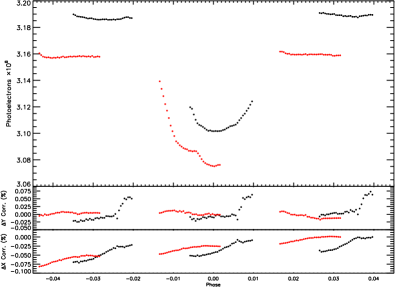
Figure 1: (Top) Raw STIS white light curve for visit 1 (black) and visit 2 (red). Three HST spacecraft orbits per visit are plotted with the transit visible in the middle orbit. The bottom two plots show the detector position systematic trends used to correct the photometric timeseries in conjunction with the HST orbital phase.

2.2 Stellar Activity Monitoring

The star HD 189733 is an active K dwarf with a rotation period of about 12 days and a flux variable at the 1-2 percent level. Monitoring the behaviour of the activity around the time of the HST visit is essential to obtain the maximum amount of information from the STIS spectroscopic time series.

The ground-based coverage was provided by the T10 0.8 m Automated Photoelectric Telescope (APT) at Fairborn Observatory in southern Arizona and spans all of our HST visits (see Fig. 2). This ongoing observing campaign of HD189733 began in October 2005 and is detailed in Henry & Winn (2008). The APT uses two photomultiplier tubes to simultaneously gather Stromgren $b$ and $y$ photometry. This dataset also covers the HD189733 stellar activity during the epochs of the HST transmission spectra from Pont et al. (2007), Swain, Vasisht & Tinetti (2008) and Sing et al. (2009), and as well as the Spitzer transit photometry of Désert et al. (2009), Knutson et al. (2009), and Désert et al. (2011). This makes this dataset an invaluable resource when comparing the stellar activity levels from epoch to epoch.

Around the first HST visit in our data, photometric coverage was also obtained with the 40-inch telescope at Wise Observatory (Israel). 25 measurements were obtained over 45 days (JD=2455130-2455171) with an $R$ filter. This was done in order to ensure photometric coverage in case of bad weather at either site, and to verify the photometric accuracy of the monitoring.

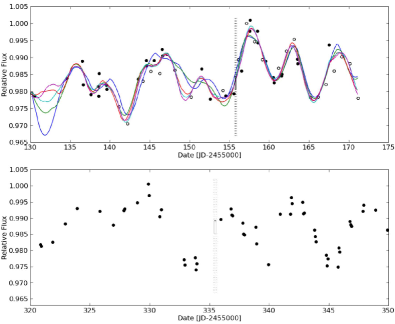
Figure 2: APT (filled circles) and Wise (open circles) photometry for HD 189733 for HST visit 1 (top) and visit 2 (bottom). Visit 1 has five representative many-spot variability models overplotted. The HST dates of both visits are indicated with the dashed lines, along with the estimated stellar flux levels at that epoch (boxes).

3 ANALYSIS

We modeled the whitelight transit light curves with the analytical transit models of Mandel & Agol (2002), choosing to fix the central transit time, planet-to-star radius contrast, inclination, and stellar density while fitting for the planet-to-star radius contrast, stellar baseline flux, and instrument systematic trends. The system parameters have been very accurately measured from the high S/N transit light curves of HST and Spitzer (Pont et al., 2007; Sing et al., 2009; Agol et al., 2010; Désert et al., 2011), and we used those of Agol et al. (2010) for this study, taken at the longest wavelength. The errors on each datapoint were set to the tabulated values which is dominated by photon noise but also includes background subtraction and readout noise. The best fit parameters were determined simultaneously with a Levenberg-Marquardt least-squares algorithm (Markwardt, 2009) using the unbinned data. The uncertainties for each fit parameter are rescaled to include any measured red noise (see Sec. 3.4) as well as non-unity reduced $\chi^{2}$ values, taking into account any underestimated errors in the tabulated datapoints. We find that the tabulated per-exposure errors are accurate at small wavelength bin sizes, but are in general an underestimation for the larger bin sizes used in this study. A few deviant points from each light curve were cut at the 3-$\sigma$ level in the residuals, and the in-transit sections obviously crossing stellar spots were also initially removed in the fits. In visit 1, the beginning 3 exposures of the in-transit orbit show an obvious spot-crossing. In visit 2, there is a large $\sim$2-4 mmag spot-like featured centered near phase $-$0.005 (see Fig. 3).

3.1 Instrument Systematic Trends

As in past STIS studies, we applied orbit-to-orbit flux corrections by fitting for a fourth-order polynomial to the photometric time series, phased on the HST orbital period. The systematic trends were fit simultaneously with the transit parameters in the fit. Higher-order polynomial fits were not statistically justified, based upon the Bayesian information criteria (BIC; Schwarz 1978). Compared to the standard $\chi^{2}$, the BIC penalizes models with larger numbers of free parameters, giving a useful criterion to help select between different models with different numbers of free parameters, and helps ensure that the preferred model does not overfit the data. The baseline flux level of each visit was let free to vary in time linearly, described by two fit parameters. In addition, we found it useful to also fit for further systematic trends which correlated with the detector position of the spectra, as determined from a linear spectral trace in IRAF and the dispersion-direction sub-pixel shift between spectral exposures, measured by cross-correlation.

We found that fitting the systematic trends with a fourth-order polynomial HST orbital period correction and linear baseline limited S/N values to the range of 9,000 to 10,000 (precisions levels of 0.011 to 0.01%). These limiting values match similar previous pre-SM4 STIS observations of HD 209458b, which also similarly corrected for these systematic trends (Brown, 2001; Knutson et al., 2007b; Ballester, Sing & Herbert, 2007; Sing et al., 2008a). With the additional correction of position related trends (see Fig. 1), were able to increase the extracted S/N to values of 14,000 per image, which is $\sim$80% of the Poisson-limited value. These additional free parameters in the fit are also justified by the BIC as well as a reduced $\chi_{\nu}^{2}$ value. In a fit excluding the position dependent systematic trends for the first STIS visit, we find a BIC value of 277 from a fit with 73 Degrees of Freedom (DOF), 8 free parameters, and a reduced $\chi_{\nu}^{2}$ of 3.31. Including the position-related trends lowers the BIC value to 202 from a fit with 70 DOF, 11 free parameters, and a reduced $\chi_{\nu}^{2}$ of 2.19. In the final whitelight curve fits, the uncertainty in fitting for instrument-related systematic trends accounts for $\sim$20% of the final $R_{\rm pl}/R_{\rm star}$ error budget.

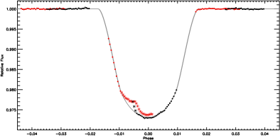
Figure 3: STIS white light curve for visit 1 (black) and visit 2 (red) with the instrument trends removed. The points showing occulted spot features are indicated with boxes. The best fit transit models for both visits are shown in grey using the un-spotted points.

3.2 Limb Darkening

At near-UV and blue optical wavelengths, the stellar limb-darkening is strong, and in general not well reproduced by standard 1D stellar atmospheric models. We account for the strong near-UV and optical limb darkening following three different prescriptions; fitting for the limb-darkening coefficients, computing limb-darkening coefficients with 1D stellar atmospheric models, and finally using a fully 3D time-dependent hydrodynamic stellar atmospheric model. We computed limb-darkening coefficients for the linear law

$$\frac{I(\mu)}{I(1)}=1-u(1-\mu)$$ (1)

as well as the Claret (2000) four-parameter limb-darkening law

$$\frac{I(\mu)}{I(1)}=1-c_{1}(1-\mu^{1/2})-c_{2}(1-\mu)-c_{3}(1-\mu^{3/2})-c_{4}(1-\mu^{2}).$$ (2)

For the 1D models, we followed the procedures of Sing (2010) using 1D Kurucz ATLAS models and the transmission function of the G430L grating (see Table 1). The four-parameters law is the best representation of the stellar model intensity distribution itself, while the linear law is the most useful in this study when fitting for the coefficients from the transit light curves.

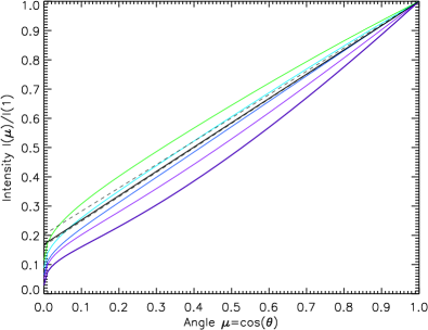
Figure 4: Stellar limb-darkening intensity profile for the STIS G430L whitelight curve (black - linear law) and spectral bandwidths (coloured - 4-parameter law) for the 3D stellar model. Also shown is the $\pm 1-\sigma$ envelope of the best-fit linear limb-darkening coefficient from the whitelight transit light curve (dashed lines).

We constructed a 3D time-dependent hydrodynamical model atmosphere using the StaggerCode (Nordlund & Galsgaard, 1995) with a resolution of $240^{3}$ grid points, spanning $4\mathrm{\,Mm}\times 4\mathrm{\,Mm}$ on the horizontal axes and $2.2$ Mm on the vertical axis. The simulation has a time-average effective temperature $\left<T_{\mathrm{eff}}\right>=5050$ K, surface gravity $\log g=4.53$ and metallicity $\mathrm{[Fe/H]}=0.0$ (based on the solar composition of Asplund, Grevesse & Sauval, 2005), which is close to the stellar parameters of Bouchy et al. (2005). Full 3D radiative transfer was computed in local thermodynamic equilibrium (LTE) based on continuous and spectral line opacities provided by Trampedach (2011, in prep.) and B. Plez (priv. comm.); see also Gustafsson et al. (2008). We obtain monochromatic surface intensities $I_{\lambda}(\mu,\phi,x,y,t)$ with a sampling of $\lambda/\Delta\lambda=20000$ in wavelength for 17 polar angles $\mu$, 4 azimuthal angles $\phi$ and a time-series of 10 snapshots that span $\approx 30$ minutes of stellar time t, with a horizontal resolution of 120 $\times$ 120 grid points in x and y. Limb darkening laws $I(\mu)/I(1)$ (see Fig. 4) were derived by averaging $I_{\lambda}(\mu,\phi,x,y,t)$ over horizontal grid, azimuth angle and time, providing a statistical representation of the surface granulation, and integrating over each bandpass and the transmission function; the result was normalized to the disk-centre intensity at $\mu=1$. A more detailed description of the 3D model will be given in a forthcoming paper by WH.

Table 1: Linear and four-parameter limb darkening coefficients for HST STIS G430L

Wavelength	transit-fit	1D model	3D model	3D model four-parameter law
(Å)	$u_{fit}$	$u_{1D}$	$u_{3D}$	$c_{1}$	$c_{2}$	$c_{3}$	$c_{4}$
2900-5700	0.816$\pm$0.019	0.8326	0.8305	0.5569	-0.4209	1.2731	-0.4963
2900-3700	1.01$\pm$0.03	0.9117	0.9534	0.5472	-0.9237	1.7727	-0.4254
3700-4200	0.91$\pm$0.01	0.9155	0.9000	0.5836	-0.8102	1.7148	-0.5389
4200-4700	0.86$\pm$0.02	0.8927	0.8680	0.5089	-0.4084	1.3634	-0.5302
4700-5200	0.80$\pm$0.02	0.7484	0.8257	0.5282	-0.3141	1.1931	-0.4994
5200-5700	0.72$\pm$0.02	0.7612	0.7701	0.6158	-0.3460	1.0695	-0.4578

While limb-darkening is stronger at near-UV and blue wavelengths, compared to the red and near-IR, the white-light stellar intensity profile is also predicted to be close to linear (see Fig. 4). Fortunately, a linear stellar intensity profile makes it much easier to compare fit limb-darkening coefficients to model values, because it is less ambiguous as to which limb-darkening law to choose and because the fit is not complicated by degeneracies when fitting for multiple limb-darkening coefficients. In the white light curve fits, we performed fits allowing the linear coefficient term to vary freely, as well as fits setting the coefficients to their 1D and 3D predicted values with the four-parameter law. The resulting coefficients are given in Table 1. Given the phase coverage between our two HST visits, and the observed occulted stellar spots in each visit, it is much more straightforward to compare model limb-darkening from visit 1, which is largely occulted-spot free. Using the linear limb-darkening law, we find $u_{fit,white}=0.816\pm 0.019$ for visit 1 (see Table 1). The fit coefficient is within 1-sigma of an appropriate ATLAS model ($u_{1Dmodel}=0.8326$ for T_eff=5000 K, log g=4.5, [Fe/H]=0.0, and $v_{turb}=2km/s$) and within 1-sigma of the 3D model, which predicts $u_{3D}=0.8305$. For visit 1, the freely fit linear limb-darkening model gives a $\chi^{2}$ value of 265 for 78 Degrees of Freedom (DOF) giving a BIC value of 315. We find that the fit is significantly worse when adopting the 1D ATLAS models with the four-parameter law, with a $\chi^{2}$ value of 286 for 79 DOF and a BIC value of 331. Using the coefficients derived from the 3D time-dependent hydrodynamical model provides an equally good fit as the linearly-fit model, with a $\chi^{2}$ value of 27 for 79 DOF and a BIC of 315. The improvement from the 1D model to the 3D model is clear, with the 3D model providing a much better fit to the transit light curve. Using the BIC as a guide, the 3D model also performs just as well as the freely fit linear limb-darkening law.

Table 2: Visit 1 transit light curve fits.

Wavelength	fit limb-darkening			3D limb-darkening
(Å)	$\chi^{2}$	DOF	BIC	$\chi^{2}$	DOF	BIC
2900-3700	208	83	258	201	84	247
3700-4200	116	82	166	115	83	160
4200-4700	132	82	182	132	83	177
4700-5200	161	83	211	162	84	207
5200-5700	114	82	164	119	83	164

As a further test, we also tried fitting a quadratic limb-darkening law, fitting for both coefficients ($u_{+}$ and $u_{-}$ in a minimally correlated manner) but found no significant improvement, as the quadratic term was not particularly well constrained from our observations.

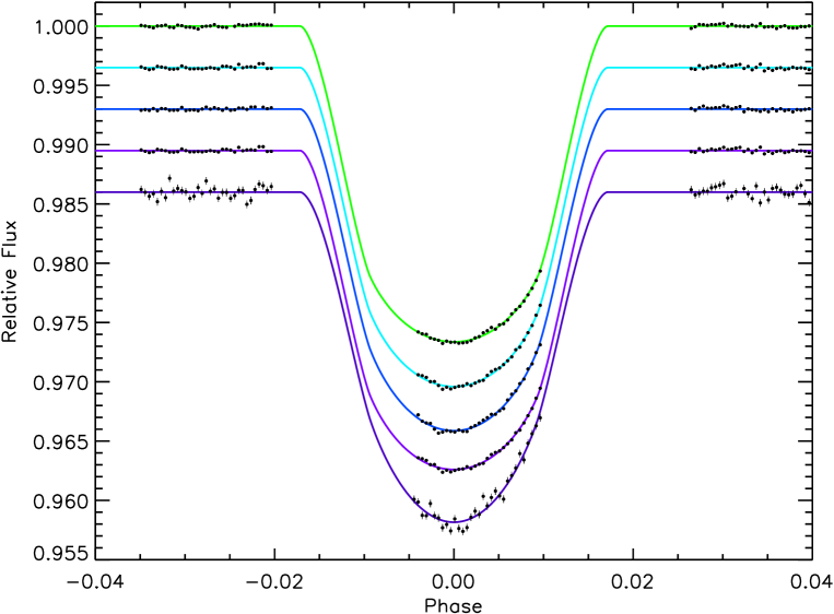
Figure 5: STIS G430L visit1 lightcurves at (bottom to top) 3300, 3950, 4450, 4950, and 5450 Å used to derive the planetary radius. The lightcurves have been corrected for instrumental effects and the first few exposures of the transit affected by occulted starspots have been removed. An arbitrary flux offset has been applied and instrumental trends removed for clarity. The best-fit transit light curve models are also overplotted.

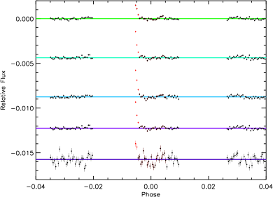
Figure 6: STIS G430L visit1 lightcurve residuals at (bottom to top) 3300, 3950, 4450, 4950, and 5450 Å with an arbitrary offset. Occulted-spot features not used in the fit are shown in red.

3.3 Transmission Spectrum Fits

To measure the broad transmission spectral features and compare them with the previous ACS results, we also extracted 500 Å wide spectral bins from the spectral time series (see Fig. 5 and Fig. 6). The resulting five bands were analyzed and individually fit in the same manner as the white light curve fits. Comparing transit fits using freely fit limb-darkening coefficients to those set of the 3D model, significant overall improvement is seen with the 3D model (see Table 2). As in the whitelight curve tests, the 3D model also handily outperforms fits using the 1D ATLAS models. At the shortest wavelength bins, adopting the 3D model limb-darkening gives a lower $\chi^{2}$ value, even with less free parameters in the transit lightcurve fit. Given the overall excellent performance of the 3D model, we adopt the predicted four-parameter 3D model coefficients for our final light curve fits. Comparing the resulting planetary radii values between those using fit limb-darkening and the 3D model, we find similar radii values for the middle two wavelength bins starting at 4200 and 4700 Å. The bluer two wavelength bins give increasingly larger radii values when using the 3D model. This trend is repeated when using the 1D ATLAS model as well, though exaggerated in the 1D case. The better fits using the 3D models and expectation that the limb-darkening at those wavelengths is significantly non-linear, indicates that larger planetary radii values toward the blue are highly likely, though some caution is in order, as these are the very first results using limb-darkening from a 3D stellar model. Such models will no doubt need further vetting at other wavelengths and against other datasets before firm confidence is ascertained. However, the overall improvement of the stellar limb-darkening from the 1D model to the 3D model is very encouraging, and very much in line with existing tests comparing such models to the Sun (see Asplund et al. 2009 and Sing et al. 2008a). There is a broad overall trend of 1D models over predicting the strength of limb-darkening compared to 3D models and solar data, due primarily to a steeper atmospheric temperature gradient in the 1D case. In 3D solar model atmospheres, convective motions lead to a shallower mean temperature profile near the surface and therefore to an overall slightly weaker predicted limb-darkening. The resulting planetary radius ratios from visit 1 are given in Table 3, which use the 3D model limb-darkening four-parameter law coefficients of Table 1. A similar transmission spectral shape is also obtained if the 1D model limb-darkening is used.

The large spot feature in visit 2 appears to affect most of the measurements between second and third contact, making it less straightforward to measure the planetary radii. We find that the planetary radius values of visit 2 are all in agreement with those from visit 1, when fitting for the visit 2 radii using the unaffected datapoints during ingress and a few points after second contact, fixing the limb-darkening to the 3D model coefficients (see Fig. 3). In Section 3.5 we describe a procedure used for visit 2 to fit for the occulted-spot and determine the wavelength-dependent planetary radii.

3.4 Noise Estimate

We checked for the presence of systematic errors correlated in time (“red noise”) by checking whether the binned residuals followed a $N^{-1/2}$ relation when binning in time by N points. In the presence of red noise, the variance can be modeled to follow a $\sigma^{2}=\sigma_{w}^{2}/N+\sigma_{r}^{2}$ relation, where $\sigma_{w}$ is the uncorrelated white noise component, while $\sigma_{r}$ characterizes the red noise (Pont, Zucker & Queloz, 2006). We found no significant evidence for red noise in the highest S/N lightcurves of visit 2 when binning on timescales up to 15 minutes (10 exposures). In visit 1 we found low levels of residual systematic errors, with $\sigma_{r}$ values around 2.5$\times 10^{-5}$, which corresponds to a limiting S/N level of $\sim$40,000. We subsequently rescaled the photometric errors to incorporate the measured values of $\sigma_{r}$ in the 1$\sigma$ error bars of the whitelight and spectral bin fits. The remaining low levels of systematic trends in visit 1 do not have a significant effect on our final transmission spectrum. A limiting precision of 2.5$\times 10^{-5}$ translates into a limiting value of 8$\times 10^{-4}$ $R_{\rm pl}/R_{\rm star}$, which is $\sim$5 times smaller than the atmospheric scale height at 1340 K.

3.5 CORRECTING FOR THE STELLAR ACTIVITY

A transmission spectrum for a transiting planet with an active host star can be affected by the presence of stellar spots, both by spots occulted by the planet and by non-occulted spots visible during the epoch of the transit observations (Pont et al., 2008; Agol et al., 2010). When the planet masks a starspot on the surface of the star during a transit (“occulted spot”), the flux rises proportionally to the dimming effect of the spot on the total stellar flux. The presence of a starspot in a region of the stellar disc not crossed by the planet (“unocculted spot”) causes a difference in surface brightness between the masked and visible parts of the stellar disc, slightly modifying the relation between transit depth and planet-to-star radius ratio. In both cases the effect is wavelength-dependent and must be corrected to obtain the planetary transmission spectrum.

Fortunately, in our observations these effects can be adequately corrected. The lightcurves are precise enough for the spot crossing events to be clearly identified, while for reasonable assumptions on the amount of spots on HD 189733, the influence of unocculted spots on the transmission spectrum is small enough that a first-order correction is possible, using the measured flux variations of the star during the HST visits and the temperature contrast of the spots inferred from occulted spots, as already discussed in Pont et al. (2008). We describe in the following paragraphs the treatment of occulted and unocculted starspots in our analysis.

3.5.1 Occulted spots

The STIS data shows clear evidence for two spot occultations by the planet, one in each visit. The flux rise is stronger at bluer wavelengths, and the timescale of the events corresponds to the motion of the planet across features on the star, so that the interpretation in terms of a masked cooler feature on the surface of the star is natural. The first event shows only the end of an occultation, while the second shows a full occultation and can be analyzed in detail.

Previous studies of the variability of HD 189733, such as the space-based lightcurve with the MOST telescope (Croll et al., 2007) and intensive spectroscopic monitoring with the SOPHIE spectrograph (Boisse et al., 2009) show that the variability of the star can be well modeled both in flux and spectrum with cooler starspots modulated by stellar rotation. We can test this hypothesis by computing the wavelength dependence of the amplitude of the flux rise caused by the spot occultation in the second visit. For this purpose, we have fitted simultaneously the planetary transit (see Fig. 7) with a wavelength-depend radius ratio and the effect of the spot with a wavelength-dependent factor for the amplitude of the spot feature. We take the shape of the spot feature from the lightcurve integrated over all wavelengths, but let it vary by a free multiplying parameter in each of five 500 Å wavelength bands. The results are shown in Figs. 8, 9, and  10. We then compare these amplification factors to expectations for the occultation of a cooler area on a $T_{\rm eff}=5000$ K star. We assume that both the star and the spot have spectral energy distributions well described by Kurucz atmosphere models, and use spot temperatures from 3500 K to 4750 K. Figure 10 compares the observed amplification factors to the model expectations. In that case the flux rise $\Delta f_{\lambda}$ at wavelength $\lambda$ compared to a reference wavelength $\lambda_{0}$ will be

$$\Delta f_{\lambda}/\Delta f_{\lambda_{0}}=\left(1-\frac{F^{T_{\rm spot}}_{\lambda}}{F^{T_{\rm star}}_{\lambda}}\right)/\left(1-\frac{F^{T_{\rm spot}}_{\lambda_{0}}}{F^{T_{\rm star}}_{\lambda_{0}}}\right)$$ (3)

where $F^{T}_{\lambda}$ is the surface brightness of the stellar atmosphere models at temperature $T$ and wavelength $\lambda$. We also plot on the figure the results of the same procedure for the ACS visit in Pont et al. (2008).

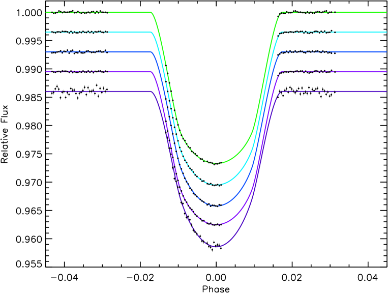
Figure 7: Same as Fig. 5 for visit2. For clarity, the occulted spot has been corrected from the lightcurves and is shown in Fig. 8.

Figure 10 shows that the spectrum of the occulted spots is well constrained, corresponding to the models with spots at least 750 K cooler than the stellar surface. Although the difference spectrum of the occulted spot is coherent with the expectation in overall shape, the 5000 Å MgH feature is weaker than expected. This does not have a significant impact on the present study, but we point it out as a possible intriguing feature of starspots on HD 189733.

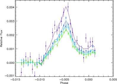
Figure 8: Plotted is the occulted spot feature from visit 2 at (top to bottom) 3300, 3950, 4450, 4950, and 5450 Å  along with the bestfit spot solution.

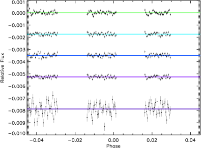
Figure 9: STIS G430L visit2 lightcurve residuals at (bottom to top) 3300, 3950, 4450, 4950, and 5450 Å with an arbitrary offset.

3.5.2 Unocculted spots

Since the timescale of spot variability is much longer than the planet crossing time during transits ($P_{\rm rot}\simeq 12$ days vs $T_{\rm tr}\simeq 1.5$ hours for HD 189733), unocculted spots can be considered as stationary during a transit, and their effect will correspond to a fixed wavelength-dependent correction on the transit depth.

As in Pont et al. (2008), we model the effects of unocculted spots by assuming that the emission spectrum of spots corresponds to a stellar spectrum of lower temperature than the rest of the star covering a fraction of the stellar surface and assuming no change in the surface brightness outside spots. We neglect the effect of faculae on the transmission spectrum. The spots then lead to an overall dimming of the star. Under these assumptions, to reach the same level of flux dimming, higher spot temperatures require a greater fraction of stellar surface covered by spots. These assumptions are now supported by the behaviour in several HST visits. The signature on the flux of occulted spots is frequently seen (to the point in fact that no entirely spot-free visit was encountered among our 9 visits), and the occulted spots observed have the expected red signature (Fig. 10; Pont et al., 2008). No detectable facula occultation is observed (a facular occultation would result in a sharp flux drop during the transit with a blue spectral signature). In Section 3.5.4 below, we present a further test in support of the validity of this assumption.

Under the assumption that the stellar flux is a combination of a surface at $T=T_{\rm star}$ and spots at $T=T_{\rm spot}$ causing a total dimming $\Delta f(\lambda_{0},t)$, the corrections to the transit depth $d$ at wavelength $\lambda$ and radius ratio due to unocculted spots will be:

$$\frac{\Delta d}{d}=\Delta f(\lambda_{0},t)\left(1-\frac{F^{T_{\rm spot}}_{\lambda}}{F^{T_{\rm star}}_{\lambda}}\right)/\left(1-\frac{F^{T_{\rm spot}}_{\lambda_{0}}}{F^{T_{\rm star}}_{\lambda_{0}}}\right)$$ (4)

and

$$\Delta(R_{\rm pl}/R_{\rm star})\simeq\frac{1}{2}\frac{\Delta d}{d}(R_{\rm pl}/R_{\rm star}).$$ (5)

A similar formalism is given in Berta et al. (2010). Figure 11 shows the correction for unocculted spots for $\Delta f(\lambda_{0},t)$=1% at $\lambda_{0}=6000$ Å for different spot temperatures. The influence over the transmission spectrum on the STIS wavelength range is of the order of $2\times 10^{-3}$ $R_{\rm pl}/R_{\rm star}$, which is $\sim$5 times smaller than the observed variations (see Section 4), suggesting that the uncertainties on the first-order correction for unocculted spots only add a small contribution to the final errors on the planetary transmission spectrum (Pont et al. 2008).

To apply the correction for unocculted spot, we need the following quantities:

1. the variation in spot dimming $\Delta f(\lambda_{0},t)$ between the different HST visits

2. an estimate of the absolute level of the stellar flux corresponding to a spot-free surface $f(\lambda_{0},t_{\rm ACS})$

3. an estimate of the effective temperature of the spots $T_{\rm spots}$

(i)Visit-to-visit flux variations

We analyzed the ground-based photometric data with a spotted star model using the same approach as in Pont, Aigrain & Zucker (2010), described in Aigrain et al. (2011). We generate a large number of evolving spots modulated by the stellar rotation, and instead of finding a unique solution that reproduces the observed photometry, we explore the space of all possible solutions. The scatter between different solutions using different number of spots and different spot parameters is used as an indicator of the uncertainty on the inferred stellar flux at a given time.

HD 189733 is now a very well-studied star, and as a result a number of key parameters for the spot simulations can be set to known values, namely the stellar size ($R=0.755$ R_⊙, Pont et al. 2007), rotation period ($P_{\rm rot}$=11.9 days, Henry & Winn 2008), and spin-orbit angle (negligible, Winn et al. 2006). Thanks to this and the excellent coverage of the photometric monitoring around the time of the HST visits, the light curve interpolation is very stable and the uncertainty on the amount of dimming by startspots at the time of the STIS measurements is not more than $2\times 10^{-3}$ (see Fig. 2).

Figure 2 gives five realizations of our many-spot model around the time of the HST visits. The number of spots used in the solution is 6, 12, 24, 48 and 96. Both the Wise and APT data are shown on the same plot, although they are taken in different filters and the amplitude of variability will be slightly different. All the solutions give very similar estimates for the brightness of the star at the moment of the first STIS/HST visit. They differ in less well-constrained part of the lightcurve, but this does not impact the present analysis. The flux in the figure is normalized to the flux at the time of the third ACS visit, used as baseline in Pont et al. (2007). Fortunately the APT coverage extends across both periods, allowing a direct comparison.

The rectangles on Fig. 2 show the values we adopted for the flux level during the STIS/HST visits. For the first visit, we use the APT level since the ($b+y$)/2 filter is near the central wavelength of the STIS measurements, while the $R$ filter used in the Wise measurements is redder. Section 3.5.4 provides an independent check of the validity of the spot-coverage estimates from the photometric monitoring, showing that the variations in observed transit depths are in close agreements with the expected variations.

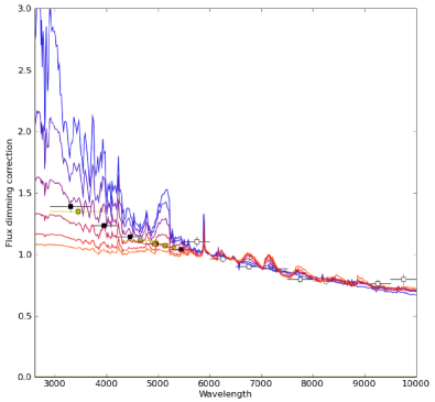
Figure 10: Spectral signature of the stellar spots occultation derived from the STIS G430L (closed black and green symbols) and ACS (open symbols) data. The spot is modeled with stellar atmospheric models of different temperatures ranging from 4750 to 3500 K in 250 K intervals (blue to orange respectively), and $T_{\rm eff}=5000$ K for the stellar temperature.

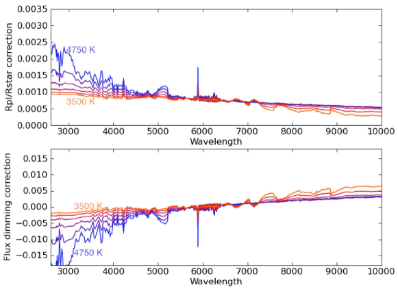
Figure 11: (Top) The effect of spot coverage on the transmission spectrum and a 1% stellar flux drop at 6000 Å where the radius ratio changes by $\Delta R_{pl}/R_{star}=0.0008$. The spot is modeled with stellar atmospheric models of different temperatures ranging from 4750 to 3500 K in 250 K intervals (blue to orange respectively), and $T_{\rm eff}=5000$ K for the stellar temperature. (Bottom) The relative stellar flux, $\Delta f_{\lambda}$, for the different spot temperatures compared to the flux at 6000 Å, assuming a 1% drop in stellar flux at that wavelength.

(ii) Flux level of spot-free surface

Pont et al. (2008) estimated the dimming level compared to a spot-free surface for the ACS visit at 1%. This component of the spot coverage is not measured by the photometric monitoring and must be inferred from the variability lightcurve. The long-term photometric monitoring with the APT over several years suggests that this value is realistic, since year-to-year variations of the maximum flux do not exceed the percent level. Pont et al. (2008; see their Fig. 2, lower-right panel) computed the effect of such a constant spot background, and the same estimates are valid for the present papers. The effect is a 200-400 km difference in transit radius (2-4$\times 10^{-3}$ on the radius ratio) per percent of stellar light blocked by the additional spot coverage over the 6000-10000 Å wavelength range. Thus, a large amount of background spot coverage would lower the blueward slope of the measured transmission spectrum.

The statistics of spot crossings on our HST data as a whole (3 visits with ACS, 2 with STIS/G430L and 4 with STIS/G750M) suggest that the global spot coverage of the star correspond to expectations from the photometric variability and do not point to a large additional spot background. The statistics of occulted starspots during the 9 visits corresponds to a flux drop of 2.8$\pm$0.8 % at $\lambda_{0}$ when extrapolated to the entire star surface. This of course assumes that the planet crossings sample a representative part of the star. The planetary transits cover the $29-55^{o}$ latitude interval. On the Sun, it is wellknown that spots cluster at low latitude. However, spots for more active stars are found to be distributed at higher latitudes than on the Sun, and cover a larger latitude range (e.g. Berdyugina & Henry 2007).

Nevertheless, when considering the transmission spectrum of HD 189733 over a wider wavelength range - for instance when comparing the visible effective radius with the values observed in the mid-infrared with Spitzer (e.g. Agol et al. 2010) this source of uncertainty should be considered.

(iii) Spot temperature

Pont et al. (2008) found that the spectral signature of the largest spot feature occulted during the ACS visit was well described by assigning $T\sim 4000$ K to the spot. In Section 3.5.1 above we found $T\sim 4250$ K for the spot occulted during our second STIS visit. Fig. 10 shows that spot temperatures in this range describe the effect of both occulted spots adequately. Spot-to-star temperature differences in this range are compatible with what is measured for solar spots.

3.5.3 Correcting for unocculted spots

We used Kurucz stellar atmosphere models to compute the unocculted spot corrections. Following the discussion above, we use $T_{\rm spot}=4250\pm 250$ K and a spot-free flux level 1.0-2.8 % above the ACS visit flux. We apply this correction to compute the planetary atmosphere transmission spectrum and propagate the uncertainties in the correction. Figure 11 shows the effect of unocculted starspots amounting to a 1-percent dimming at 6000 Å on the transmission spectrum, and Table 4 gives the corrections as a fraction of transit depth integrated over 500 Å passbands. Overall, the effect is very small, but not negligible in the context of the highly accurate HST transmission spectroscopy.

Table 3: Fit STIS G430L Radius Ratios in five wavelength bands and spot corrected values using Table 4 and Eq. 5 with $\Delta f(\lambda_{0},{\rm visit~{}1})$=0.017 and $\Delta f(\lambda_{0},{\rm visit~{}2})$=0.013.

$\lambda$	Visit 1	Correction	Visit 1 Corrected
(Å)	$R_{pl}/R_{star}$	$\Delta R_{pl}/R_{star}$	$R_{pl}/R_{star}$
3300	0.15985$\pm$0.00042	-0.00172	0.15813$\pm$0.00048
3950	0.15872$\pm$0.00019	-0.00161	0.15711$\pm$0.00019
4450	0.15803$\pm$0.00023	-0.00150	0.15653$\pm$0.00023
4950	0.15770$\pm$0.00022	-0.00154	0.15616$\pm$0.00022
5450	0.15744$\pm$0.00022	-0.00138	0.15606$\pm$0.00022
$\lambda$	Visit 2	Correction	Visit 2 Corrected
(Å)	$R_{pl}/R_{star}$	$\Delta R_{pl}/R_{star}$	$R_{pl}/R_{star}$
3300	0.15803$\pm$0.00050	-0.00132	0.15671$\pm$0.00056
3950	0.15796$\pm$0.00024	-0.00123	0.15673$\pm$0.00024
4450	0.15787$\pm$0.00014	-0.00144	0.15673$\pm$0.00014
4950	0.15765$\pm$0.00011	-0.00117	0.15648$\pm$0.00011
5450	0.15725$\pm$0.00012	-0.00105	0.15620$\pm$0.00012

$\lambda$	Combined
(Å)	$R_{pl}/R_{star}$
3300	0.15754$\pm$0.00042
3950	0.15696$\pm$0.00015
4450	0.15667$\pm$0.00012
4950	0.15641$\pm$0.00010
5450	0.15617$\pm$0.00011

Table 4: Unocculted spot corrections to the transmission spectrum with spot temperature T${\rm spot}=4250\pm 250$ causing 1% dimming at 6000 Å. On this scale, the absolute value of the shift is 1% of the transit depth at 6000 Å by definition.

Passband	Spot correction
(Å)	$\Delta d/d$ [$\times 10^{-3}$]
3200-3750	2.92$\pm$1.13
3750-4000	2.08$\pm$0.94
4250-4750	1.21$\pm$0.45
4750-5250	1.51$\pm$0.53
5250-5750	0.31$\pm$0.17
5750-6250	0.0$\pm$0.0

3.5.4 Empirical Radius-Activity Level Correlation

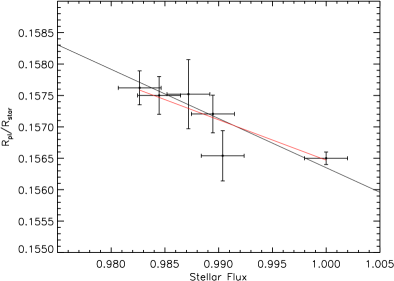
Figure 12: HST planet-to-star radius measurements ($R_{pl}/R_{star}$) between 5200 and 6100 Å from STIS G430L, STIS G750M and ACS HRC plotted against the observed stellar flux at the transit epoch. The black solid line is the predicted relation for the radius impact from stellar variability, assuming non-occulted dark stellar spots. The red line is the best-fit relation from the HST observations, which is in very good agreement with the prediction.

Between the ACS measurements, the two STIS visits presented here, and three HD189733b transits obtained with the STIS G750M as part of a separate HST program (GO 11572, PI D. Sing), there are now sufficiently similar high S/N transit optical observations to search for the expected correlation in Eq. 3 between the measured transit radius ratio and the activity levels of the star. To search for this correlation, we used the non-contaminated G430L visit 1 and visit 2 data at the reddest wavelength bin (5200-5700 Å), along with the whitelight curves of three similarly high S/N G750M transits (5880-6200 Å), estimating the stellar flux level at each transit epoch from the APT data. We also used the shortest wavelength ACS radius, applying a small correction such that the inclination and impact parameters match those of Agol et al. (2010), also used for the STIS transits. As each STIS transit is well sampled temporally, we can fit for the radius ratio of each transit using only occulted-spot free regions. The results are plotted in Fig. 12. A linear fit between the flux and radius gives as slope of $\Delta(R_{\rm pl}/R_{\rm star})/\Delta f(\lambda_{0},t)=-$0.064$\pm$0.016, in excellent agreement with the theoretically predicted slope value of $-\frac{1}{2}(R_{\rm pl}/R_{\rm star})=-$0.078 from Eq. 4 and 5, and the expectation of stellar variability via dark stellar spots. This correlation reinforces the importance and usefulness of ground-based monitoring for active transiting hosting stars, and lends credence to the hypothesis that in sufficiently non-active stars, such stellar activity related radius changes can be negligible (Sing et al., 2011).

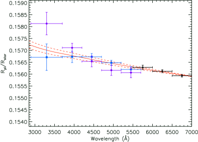
Figure 13: G430L transit radius spectrum for visit 1 (purple circles) and visit 2 (blue squares) along with previous ACS measurements (black squares) and the prediction from Rayleigh scattering (solid and dashed lines). The wavelength bins are indicated by the X-axis error bar size and the 1-$\sigma$ error of the transit fit is indicated by the Y-axis error bar size.

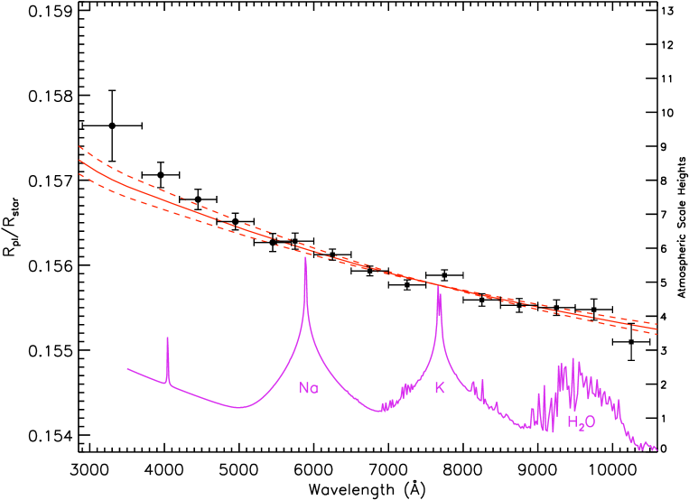
Figure 14: STIS and ACS transmission spectra for HD189733b. Plotted blue-ward of 5600 Å is the STIS G430L measurements (circles) with the ACS measurements from Pont et al. (2008) red-ward of 5600 Å(squares). The wavelength bins are indicated by the X-axis error bars and the 1-$\sigma$ error is indicated by the Y-axis error bars. The right Y-axis is labeled in units of estimated atmospheric scale heights, assuming T=1340 K ($H$=0.0004 $R_{pl}/R_{star}$). The prediction from ACS Rayleigh scattering (1340$\pm$150 K red solid and dashed lines) is also shown, as is a haze-free model atmosphere for HD 189733b from Fortney et al. (2010, Fig. 7) which uses a planet-wide average T-P profile, and is normalized to the radii at infrared wavelengths.

4 DISCUSSION

We find very good overall agreement between the transmission spectrum of the two HST visits for HD189733b (see Fig. 13, Table 3). The largest deviation (at the 2-$\sigma$ level) is at the very bluest wavelength, which is most sensitive to the prescriptions used for limb-darkening, as well as the occulted stellar spot fits of visit 2. The average transmission spectrum we obtain (see Fig. 14) between 4200 and 5700 Å is featureless, lacking the broad Na and K absorption lines, with a blue-ward slope similar to the ACS measurements. Like the ACS spectrum (but unlike HD209458b) we find no evidence for the wide pressure-broadened sodium wings (e.g. Fortney et al. 2010), though there is good evidence that the sodium line core is present both from ground based measurements (Redfield et al., 2008) as well as our G750M measurements (Huitson, Sing, in prep), which indicates that either the sodium abundance is much lower in HD189733b or more likely that the optical and near-UV transmission spectrum covers lower pressures and higher altitudes than in HD209458b. The high altitudes are also illustrated by derived planetary radii for both ACS and STIS, which are both well in excess of those observed in the near-IR and at Spitzer IRAC wavelengths. For a hydrostatic atmosphere at $\sim$1300 K, the ACS spans 2 scale heights above the 1.88$\mu$m and 8$\mu$m radii of Sing et al. (2009) and Agol et al. (2010) respectively, while the G430L spans $\sim$2 to 6 scale heights above.

The featureless slope and lack of the expected sodium and potassium alkali line wings further indicates optical atmospheric haze, as first detected by Pont et al. (2008) using HST ACS. The effective transit measured altitude $z$ of a hydrostatic atmosphere as a function of wavelength $\lambda$ was found in Lecavelier des Etangs et al. (2008a),

$$z(\lambda)=H\mathrm{ln}\left(\frac{\varepsilon_{\rm abs}P_{\rm ref}\sigma(\lambda)}{\tau_{\rm eq}}\sqrt{\frac{2\pi R_{\rm pl}}{kT\mu g}}\right),$$ (6)

where $\varepsilon_{abs}$ is the abundance of dominating absorbing species, $T$ is the atmospheric temperature at $z$, $H=kT/\mu g$ is the atmospheric scale height, $\mu$ is the mean mass of the atmospheric particles, $P_{\rm ref}$ is the pressure at the reference altitude, and $\sigma(\lambda)$ is the absorption cross section. This allows the derivation of the apparent planetary radius as a function of wavelength from the known cross section variations. Assuming a scaling law for the cross section in the form $\sigma=\sigma_{0}(\lambda/\lambda_{0})^{\alpha}$, the slope of the planet radius as a function of wavelength is given by

$$\frac{dR_{pl}}{d\ln\lambda}=\alpha H=\alpha\frac{kT}{\mu g}.$$ (7)

If the cross section as a function of wavelength is known, the local atmospheric temperature can thus be estimated by

$$\alpha T=\frac{\mu g}{k}\frac{dR_{pl}}{d\ln\lambda}.$$ (8)

For the ACS measurements, Lecavelier des Etangs et al. (2008a) showed that Rayleigh scattering with $\alpha=-4$ (Rayleigh cross section is $\sigma=\sigma_{0}(\lambda/\lambda_{0})^{-4}$) provides a temperature of 1340$\pm$150 K, consistent with other estimates. They also concluded that the absorption from atmospheric haze particles is due to Rayleigh scattering and suggested MgSiO₃ as a possible candidate; this condensate is indeed predicted to be present in hot Jupiters and brown dwarfs by Helling, Woitke & Thi (2008). MgSiO₃ is an attractive candidate over many other plausible dust condensates (like Mg₂SiO₄, MgFeSiO₄, O-deficient silicates, etc.), as the scattering efficiency dominates over absorption efficiency, giving a Rayleigh scattering profile when using the Mie approximation.

The STIS G430L measurements between 2900 and 5700 Å gives $\alpha T=$$-8400\pm 2000$ K slope. The total magnitude of the un-occulted spot correction for the visit 1 and visit 2 STIS G430L data is incorporated in the slope error and accounts for about 40% of the slope uncertainty. Assuming that Rayleigh scattering still holds at these shorter wavelengths, the steeper slope would indicate higher temperatures of 2100$\pm$500 K, following Eq. 7. Comparing the two Rayleigh temperatures between the ACS and STIS datasets, the STIS appears warmer by 760$\pm$522 K which is at the 1.5-$\sigma$ significance level.

Warmer temperatures at higher altitudes could indicate the presence of a thermosphere. Within the context of Rayleigh scattering, redder wavelengths have a lower cross section, thus the transmission spectrum would be probing somewhat deeper into the atmosphere, toward cooler temperatures below the thermosphere. A thermosphere at these high altitudes is expected and is in agreement with the detection of an escaping exosphere (Lecavelier Des Etangs et al., 2010) A similar thermosphere has also been observed at high altitudes on HD 209458b when using sodium to probe the temperature profile (Vidal-Madjar et al., 2011). Very high temperatures could potentially pose a problem for Rayleigh scattering via MgSiO₃ particles, as they vaporize near 1400 K, though the higher temperatures measured in the G430L are only marginally significant. A Rayleigh scattering dominated atmosphere would imply a high albedo, as a semi-infinite purely Rayleigh scattering atmosphere has a theoretical geometric albedo of 0.8 (Prather, 1974).

The larger radii at near-UV wavelengths (blueward of $\sim$4000 Å) could also be attributed to other absorbing features, such as a Balmer jump associated with the escaping atmosphere (Ballester, Sing & Herbert, 2007) or sulfur compounds generated photochemically (Zahnle et al., 2009). Both scenarios have significant absorption at high altitudes blueward of $\sim$4000 Å, though a larger EUV flux for HD 189733b (compared to HD 209458b) should limit a Balmer jump signature and sulfur compounds have a characteristically steeper absorption profile.

5 CONCLUSION

HD 189733b is now only the second exoplanet to have a full optical transmission spectrum measured. Using high S/N observations from the repaired STIS instrument, we confirm a featureless spectrum with opacity increasing bluewards in the optical, suggestive of Rayleigh scattering and atmospheric haze. The HST transmission spectral results indicate that the atmospheric haze and Rayleigh scattering is an important feature of HD 189733b’s atmosphere and would imply a high albedo. The effect of the haze on the global energy budget of the planet could be significant, as the wavelength-dependent albedo from Rayleigh scattering is large, while typical condensate-free hot-Jupiter atmospheres are dominated by Na and K line wings and have very low optical albedos. Such a large albedo can be independently checked by optical secondary eclipse measurements. For HD 189733b the optical secondary eclipse has yet to be measured, as the stellar activity makes it difficult to build up a detection from multiple eclipse events (Rowe et al., 2006).

The list of key differences between the two well studied hot Jupiters is growing, with HD 209458b likely featuring a low albedo, stratospheric temperature inversion, inflated planetary radius, and large Na alkali line wings while HD 189733b has a high albedo, no stratospheric temperature inversion, a non-inflated planetary radius, and a global haze covering significant alkali line wing absorption. Such differences points toward a large diversity between the broader class of hot-Jupiter atmospheres, as HD 209458b and HD 189733b only differ by a few hundred degrees K.

References

- Agol et al. (2010) Agol E., Cowan N. B., Knutson H. A., Deming D., Steffen J. H., Henry G. W., Charbonneau D., 2010, ApJ, 721, 1861
- Asplund, Grevesse & Sauval (2005) Asplund M., Grevesse N., Sauval A. J., 2005, in Astronomical Society of the Pacific Conference Series, Vol. 336, Cosmic Abundances as Records of Stellar Evolution and Nucleosynthesis, T. G. Barnes III & F. N. Bash, ed., p. 25
- Asplund et al. (2009) Asplund M., Grevesse N., Sauval A. J., Scott P., 2009, ARA & A, 47, 481
- Ballester, Sing & Herbert (2007) Ballester G. E., Sing D. K., Herbert F., 2007, Nature, 445, 511
- Berdyugina & Henry (2007) Berdyugina S. V., Henry G. W., 2007, ApJ, 659, L157
- Berta et al. (2010) Berta Z. K., Charbonneau D., Bean J., Irwin J., Burke C. J., Désert J., Nutzman P., Falco E. E., 2010, ArXiv e-prints
- Boisse et al. (2009) Boisse I. et al., 2009, A & A, 495, 959
- Bouchy et al. (2005) Bouchy F. et al., 2005, A & A, 444, L15
- Brown (2001) Brown T. M., 2001, ApJ, 553, 1006
- Burrows et al. (2007) Burrows A., Hubeny I., Budaj J., Knutson H. A., Charbonneau D., 2007, ApJ, 668, L171
- Charbonneau et al. (2002) Charbonneau D., Brown T. M., Noyes R. W., Gilliland R. L., 2002, ApJ, 568, 377
- Charbonneau et al. (2008) Charbonneau D., Knutson H. A., Barman T., Allen L. E., Mayor M., Megeath S. T., Queloz D., Udry S., 2008, ApJ, 686, 1341
- Claret (2000) Claret A., 2000, A & A, 363, 1081
- Croll et al. (2007) Croll B. et al., 2007, ApJ, 671, 2129
- Deming et al. (2005) Deming D., Seager S., Richardson L. J., Harrington J., 2005, Nature, 434, 740
- Désert et al. (2011) Désert J. et al., 2011, A & A, 526, A12
- Désert et al. (2009) Désert J.-M., Lecavelier des Etangs A., Hébrard G., Sing D. K., Ehrenreich D., Ferlet R., Vidal-Madjar A., 2009, ApJ, 699, 478
- Désert et al. (2008) Désert J.-M., Vidal-Madjar A., Lecavelier des Etangs A., Sing D., Ehrenreich D., Hébrard G., Ferlet R., 2008, A & A, 492, 585
- Fortney et al. (2008) Fortney J. J., Lodders K., Marley M. S., Freedman R. S., 2008, ApJ, 678, 1419
- Fortney et al. (2010) Fortney J. J., Shabram M., Showman A. P., Lian Y., Freedman R. S., Marley M. S., Lewis N. K., 2010, ApJ, 709, 1396
- Grillmair et al. (2008) Grillmair C. J. et al., 2008, Nature, 456, 767
- Gustafsson et al. (2008) Gustafsson B., Edvardsson B., Eriksson K., Jørgensen U. G., Nordlund Å., Plez B., 2008, A & A, 486, 951
- Helling, Woitke & Thi (2008) Helling C., Woitke P., Thi W., 2008, A & A, 485, 547
- Henry & Winn (2008) Henry G. W., Winn J. N., 2008, AJ, 135, 68
- Knutson et al. (2009) Knutson H. et al., 2009, ApJ, 690, 822
- Knutson et al. (2008) Knutson H. A., Charbonneau D., Allen L. E., Burrows A., Megeath S. T., 2008, ApJ, 673, 526
- Knutson et al. (2007a) Knutson H. A. et al., 2007a, Nature, 447, 183
- Knutson et al. (2007b) Knutson H. A., Charbonneau D., Noyes R. W., Brown T. M., Gilliland R. L., 2007b, ApJ, 655, 564
- Lecavelier Des Etangs et al. (2010) Lecavelier Des Etangs A. et al., 2010, A & A, 514, A72
- Lecavelier des Etangs et al. (2008a) Lecavelier des Etangs A., Pont F., Vidal-Madjar A., Sing D., 2008a, A & A, 481, L83
- Lecavelier des Etangs et al. (2008b) Lecavelier des Etangs A., Vidal-Madjar A., Désert J.-M., Sing D., 2008b, A & A, 485, 865
- Linsky et al. (2010) Linsky J. L., Yang H., France K., Froning C. S., Green J. C., Stocke J. T., Osterman S. N., 2010, ApJ, 717, 1291
- Mandel & Agol (2002) Mandel K., Agol E., 2002, ApJ, 580, L171
- Markwardt (2009) Markwardt C. B., 2009, in Astronomical Society of the Pacific Conference Series, D. A. Bohlender, D. Durand, & P. Dowler, ed., Vol. 411, p. 251
- Nordlund & Galsgaard (1995) Nordlund Å., Galsgaard K., 1995, A 3d MHD code for parallel computers. Tech. rep., Astronomical Observatory, Copenhagen University
- Pont, Aigrain & Zucker (2010) Pont F., Aigrain S., Zucker S., 2010, ArXiv e-prints
- Pont et al. (2007) Pont F. et al., 2007, A & A, 476, 1347
- Pont et al. (2008) Pont F., Knutson H., Gilliland R. L., Moutou C., Charbonneau D., 2008, MNRAS, 385, 109
- Pont, Zucker & Queloz (2006) Pont F., Zucker S., Queloz D., 2006, MNRAS, 373, 231
- Prather (1974) Prather M. J., 1974, ApJ, 192, 787
- Redfield et al. (2008) Redfield S., Endl M., Cochran W. D., Koesterke L., 2008, ApJ, 673, L87
- Rogers et al. (2009) Rogers J. C., Apai D., López-Morales M., Sing D. K., Burrows A., 2009, ApJ, 707, 1707
- Rowe et al. (2006) Rowe J. F. et al., 2006, ApJ, 646, 1241
- Schwarz (1978) Schwarz G., 1978, Ann. Statistics, 6, 461
- Sing (2010) Sing D. K., 2010, A & A, 510, A21
- Sing et al. (2011) Sing D. K. et al., 2011, A & A, 527, A73
- Sing et al. (2009) Sing D. K., Désert J., Lecavelier Des Etangs A., Ballester G. E., Vidal-Madjar A., Parmentier V., Hebrard G., Henry G. W., 2009, A & A, 505, 891
- Sing & López-Morales (2009) Sing D. K., López-Morales M., 2009, A & A, 493, L31
- Sing et al. (2008a) Sing D. K., Vidal-Madjar A., Désert J.-M., Lecavelier des Etangs A., Ballester G., 2008a, ApJ, 686, 658
- Sing et al. (2008b) Sing D. K., Vidal-Madjar A., Lecavelier des Etangs A., Désert J.-M., Ballester G., Ehrenreich D., 2008b, ApJ, 686, 667
- Snellen et al. (2008) Snellen I. A. G., Albrecht S., de Mooij E. J. W., Le Poole R. S., 2008, A & A, 487, 357
- Snellen et al. (2010) Snellen I. A. G., de Kok R. J., de Mooij E. J. W., Albrecht S., 2010, Nature, 465, 1049
- Swain, Vasisht & Tinetti (2008) Swain M. R., Vasisht G., Tinetti G., 2008, Nature, 452, 329
- Swain et al. (2009) Swain M. R., Vasisht G., Tinetti G., Bouwman J., Chen P., Yung Y., Deming D., Deroo P., 2009, ApJ, 690, L114
- Vidal-Madjar et al. (2004) Vidal-Madjar A. et al., 2004, ApJ, 604, L69
- Vidal-Madjar et al. (2003) Vidal-Madjar A., Lecavelier des Etangs A., Désert J.-M., Ballester G. E., Ferlet R., Hébrard G., Mayor M., 2003, Nature, 422, 143
- Vidal-Madjar et al. (2011) Vidal-Madjar A. et al., 2011, A & A, 527, A110
- Winn et al. (2006) Winn J. N. et al., 2006, ApJ, 653, L69
- Zahnle et al. (2009) Zahnle K., Marley M. S., Freedman R. S., Lodders K., Fortney J. J., 2009, ApJ, 701, L20