Inverse Queries For Multidimensional Spaces

Abstract

Traditional spatial queries return, for a given query object $q$, all database objects that satisfy a given predicate, such as epsilon range and $k$-nearest neighbors. This paper defines and studies inverse spatial queries, which, given a subset of database objects $Q$ and a query predicate, return all objects which, if used as query objects with the predicate, contain $Q$ in their result. We first show a straightforward solution for answering inverse spatial queries for any query predicate. Then, we propose a filter-and-refinement framework that can be used to improve efficiency. We show how to apply this framework on a variety of inverse queries, using appropriate space pruning strategies. In particular, we propose solutions for inverse epsilon range queries, inverse $k$-nearest neighbor queries, and inverse skyline queries. Our experiments show that our framework is significantly more efficient than naive approaches.

1 Introduction

Recently, a lot of interest has grown for reverse queries, which take as input an object $o$ and find the queries which have $o$ in their result set. A characteristic example is the reverse $k$NN query [5, 9], whose objective is to find the query objects (from a given dataset) that have a given input object in their $k$NN set. In such an operation the roles of the query and data objects are reversed; while the $k$NN query finds the data objects which are the nearest neighbors of a given query object, the reverse query finds the objects which, if used as queries, return a given data object in their result. Besides $k$NN search, reverse queries have also been studied for other spatial and multidimensional search problems, such as top-$k$ search [10] and dynamic skyline [6]. Reverse queries mainly find application in data analysis tasks; e.g., given a product find the customer searches that have this product in their result. [5] outlines a wide range of such applications (including business impact analysis, referral and recommendation systems, maintenance of document repositories).

In this paper, we generalize the concept of reverse queries. We note that the current definitions take as input a single object. However, similarity queries such as $k$NN queries and $\varepsilon$-range queries may in general return more than one result. Data analysts are often interested in the queries that include two or more given objects in their result. Such information can be meaningful in applications where only the result of a query can be (partially) observed, but the actual query object is not known. For example consider an online shop selling a variety of different products stored in a database $\mathcal{D}$. The online shop may be interested in offering a package of products $Q\subseteq\mathcal{D}$ for a special price. The problem at hand is to identify customers which are interested in all items of the package, in order to direct an advertisement to them. We assume that the preferences of registered customers are known. First, we need to define a predicate indicating whether a user is interested in a product. A customer may be interested in a product if

• the distance between the product’s features and the customer’s preference is less than a threshold $\varepsilon$.

• the product is contained in the set of his $k$ favorite items, i.e., the $k$-set of product features closest to the user’s preferences.

• the product is contained in the customer’s dynamic skyline, i.e., there is no other product that better fits the customer’s preferences in every possible way.

Therefore, we want to identify customers $r$, such that the query on $\mathcal{D}$ with query object $r$, using one of the query predicates above, contains $Q$ in the result set. More specifically, consider a set $\mathcal{D}\in\mathbb{R}^{d}$ as a database of $n$ objects and let $d(\cdot)$ denote the Euclidean distance in $\mathbb{R}^{d}$. Let ${\mathcal{P}}(q)$ be a query on $\mathcal{D}$ with predicate ${\mathcal{P}}$ and query object $q$.

Definition 1

An inverse ${\mathcal{P}}$ query (I${\mathcal{P}}$Q) computes for a given set of query objects $Q\subseteq\mathcal{D}$ the set of points $r\in\mathbb{R}^{d}$ for which $Q$ is in the ${\mathcal{P}}$ query result; formally:

$$I{\mathcal{P}}Q=\{r\in\mathbb{R}^{d}:Q\subseteq{\mathcal{P}}(r))\}$$

Simply speaking, the result of the general inverse query is the subset of the space defined by all objects $r$ for which all $Q$-objects are in ${\mathcal{P}}(r)$. Special cases of the query are

• The mono-chromatic inverse ${\mathcal{P}}$ Query, for which the result set is a subset of $\mathcal{D}$.

• The bi-chromatic inverse ${\mathcal{P}}$ Query, for which the result set is a subset of a given database $\mathcal{D}^{\prime}\subseteq\mathbb{R}^{d}$.

In this paper, we study the inverse versions of three common query types in spatial and multimedia databases as follows.

(a) $I\varepsilon\mbox{-}RQ$.

(b) $Ik\mbox{-}NNQ$, $k=3$.

Figure 1: Examples of inverse queries.

Inverse $\varepsilon$-Range Query ($I\varepsilon\mbox{-}RQ$). The inverse $\varepsilon$-Range query returns all objects which have a sufficiently low distance to all query objects. For a bi-chromatic sample application of this type of query, consider a movie database containing a large number of movie records. Each movie record contains features such as humor, suspense, romance, etc. Users of the database are represented by the same attributes, describing their preferences. We want to create a recommendation system that recommends to users movies that are sufficiently similar to their preferences (i.e., distance less than $\varepsilon$). Now, assume that a group of users, such as a family, want to watch a movie together; a bi-chromatic $I\varepsilon\mbox{-}RQ$ query will recommend movies which are similar to all members of the family. For a mono-chromatic case example, consider the set $Q=\{q_{1},q_{2}\}$ of query objects of Figure 1(a) and the set of database points $\mathcal{D}=\{p_{1},p_{2},\cdots,p_{6}\}$. If the range $\varepsilon$ is as illustrated in the figure, the result of the $I\varepsilon\mbox{-}RQ(Q)$ is $\{p_{2},p_{4},p_{5}\}$ (e.g., $p_{1}$ is dropped because $d(p_{1},q_{2})>\varepsilon$).

Inverse $k$-NN Query ($Ik\mbox{-}NNQ$). The inverse $k$NN query returns the objects which have all query points in their $k$NN set. For example, mono-chromatic inverse $k$NN queries can be used to aid crime detection. Assume that a set of households have been robbed in short succession and the robber must be found. Assume that the robber will only rob houses which are in his close vicinity, e.g. within the closest hundred households. Under this assumption, performing an inverse $100$NN query, using the set of robbed households as $Q$, returns the set of possible suspects. A mono-chromatic inverse 3NN query for $Q=\{q_{1},q_{2}\}$ in Figure 1(b) returns $\{p_{4}\}$. $p_{6}$, for example, is dropped, as $q_{2}$ is not contained in the list of its 3 nearest neighbors.

Inverse Dynamic Skyline Query ($I\mbox{-}DSQ$). An inverse dynamic skyline query returns the objects, which have all query objects in their dynamic skyline. A sample application for the general inverse dynamic skyline query is a product recommendation problem: Assume there is a company, e.g. a photo camera company, that provides its products via an internet portal. The company wants to recommend to their customers products by analyzing the web pages visited by them. The score function used by the customer to rate the attributes of products is unknown. However, the set of products that the customer has clicked on can be seen as samples of products that he or she is interested in, and thus, must be in the customers dynamic skyline. The inverse dynamic skyline query can be used to narrow the space which the customers preferences are located in. Objects which have all clicked products in their dynamic skyline are likely to be interesting to the customer. In Figure 1, assuming that $Q=\{q_{1},q_{2}\}$ are clicked products, $I\mbox{-}DSQ(Q)$ includes $p_{6}$, since both $q_{1}$ and $q_{2}$ are included in the dynamic skyline of $p_{6}$.

For simplicity, we focus on the mono-chromatic cases of the respective query types (i.e., query points and objects are taken from the same data set); however, the proposed techniques can also be applied for the bi-chromatic (cf. Appendix 0.D) and the general case.

Motivation. A naive way to process any inverse spatial query is to compute the corresponding reverse query for each $q_{i}\in Q$ and then intersect these results. The problem of this method is that running a reverse query for each $q_{i}$ multiplies the complexity of the reverse query by $|Q|$ both in terms of computational and I/O cost. Objects that are not shared in two or more reverse queries in $Q$ are unnecessarily retrieved, while objects that are shared by two or more queries are redundantly accessed multiple times. We propose a filter-refinement framework for inverse queries, which first applies a number of filters using the set of query objects $Q$ to prune effectively objects which may not participate in the result. Afterwards candidates are pruned by considering other database objects. Finally, during a refinement step, the remaining candidates are verified against the inverse query and the results are output. Details of our framework are shown in Section 3. When applying our framework to the three inverse queries under study, filtering and refinement are sometimes integrated in the same algorithm, which performs these steps in an iterative manner. Although for $I\varepsilon\mbox{-}RQ$ queries the application of our framework is straightforward, for $Ik\mbox{-}NNQ$ and $I\mbox{-}DSQ$, we define and exploit special pruning techniques that are novel compared to the approaches used for solving the corresponding reverse queries.

Outline. The rest of the paper is organized as follows. In the next section we give an overview of the previous work which is related to inverse query processing. Section 3 describes our framework. In Sections 4-6 we implement it on the three inverse spatial query types; we first briefly introduce the pruning strategies for the single-query-object case and then show how to apply the framework in order to handle the multi-query-object case in an efficient way. Section 7 is an experimental evaluation and Section 8 concludes the paper.

2 Related Work

The problem of supporting reverse queries efficiently, i.e. the case where $Q$ only contains a single database object, has been studied extensively. However, none of the proposed approaches is directly extendable for the efficient support of inverse queries when $|Q|>1$. First, there exists no related work on reverse queries for the $\epsilon$-range query predicate. This is not surprising since the the reverse $\epsilon$-range query is equal to a (normal) $\epsilon$-range query. However, there exists a large body of work for reverse $k$-nearest neighbor (R$k$NN) queries. Self-pruning approaches like the RNN-Tree [5] and the RdNN-tree [11] operate on top of a spatial index, like the R-tree. Their objective is to estimate the $k$NN distance of each index entry $e$. If the $k$NN distance of $e$ is smaller than the distance of $e$ to the query $q$, then $e$ can be pruned. These methods suffer from the high materialization and maintenance cost of the $k$NN distances.

Mutual-pruning approaches such as [8, 7, 9] use other points to prune a given index entry $e$. TPL [9] is the most general and efficient approach. It uses an R-tree to compute a nearest neighbor ranking of the query point $q$. The key idea is to iteratively construct Voronoi hyper-planes around $q$ using the retrieved neighbors. TPL can be used for inverse $k$NN queries where $|Q|>1$, by simply performing a reverse $k$NN query for each query point and then intersecting the results (i.e., the brute-force approach).

For reverse dynamic skyline queries, [2] proposed an efficient solution, which first performs a filter-step, pruning database objects that are globally dominated by some point in the database. For the remaining points, a window query is performed in a refinement step. In addition, [6] gave a solution for reverse dynamic skyline computation on uncertain data. None of these methods considers the case of $|Q|>1$, which is the focus of our work.

In [10] the problem of reverse top-$k$ queries is studied. A reverse top-$k$ query returns for a point $q$ and a positive integer $k$, the set of linear preference functions for which $q$ is contained in their top-$k$ result. The authors provide an efficient solution for the 2D case and discuss its generalization to the multidimensional case, but do not consider the case where $|Q|>1$. Although we do not study inverse top-$k$ queries in this paper, we note that it is an interesting subject for future work.

3 Inverse Query (IQ) Framework

Our solutions for the three inverse queries under study are based on a common framework consisting of the following filter-refinement pipeline:

Filter 1: Fast Query Based Validation:

The first component of the framework, called fast query based validation, uses the set of query objects $Q$ only to perform a quick check on whether it is possible to have any result at all. In particular, this filter verifies simple constraints that are necessary conditions for a non-empty result. For example, for the I$k$NN case, the result is empty if $|Q|>k$.

Filter 2: Query Based Pruning:

Query based pruning again uses the query objects only to prune objects in $\mathcal{D}$ which may not participate in the result. Unlike the simple first filter, here we employ the topology of the query objects.

Filters 1 and 2 can be performed very fast because they do not involve any database object except the query objects.

Filter 3: Object Based Pruning:

This filter, called object based pruning, is more advanced because it involves database objects additional to the query objects. The strategy is to access database objects in ascending order of their maximum distance to any query point; formally:

$$MaxDist(o,Q)=\max_{q\in Q}(d(e,q)).$$

The rationale for this access order is that, given any query object $q$, objects that are close to $q$ have more pruning power, i.e., they are more likely to prune other objects w.r.t. $q$ than objects that are more distant to $q$. To maximize the pruning power, we prefer to examine objects that are close to all query points first.

Note that the applicability of the filters depends on the query. Query based pruning is applicable if the query objects suffice to restrict the search space which holds for the inverse $\varepsilon$-range query and the inverse skyline query but not directly for the inverse $k$NN query. In contrast, the object based pruning filter is applicable for queries where database objects can be used to prune other objects which for example holds for the inverse $k$NN query and the inverse skyline query but not for the inverse $\varepsilon$-range query.

Refinement:

In the final refinement step, the remaining candidates are verified and the true hits are reported as results.

4 Inverse $\varepsilon$-Range Query

We will start with the simpler query, the inverse $\varepsilon$-range query. First, consider the case of a query object $q$ (i.e., $|Q|=1$). In this case, the inverse $\varepsilon$-range query computes all objects, that have $q$ within their $\varepsilon$-range sphere. Due to the symmetry of the $\varepsilon$-range query predicate, all objects satisfying the inverse $\varepsilon$-range query predicate are within the $\varepsilon$-range sphere of $q$ as illustrated in Figure 2(a). In the following, we consider the general case, where $|Q|>1$ and show how our framework can be applied.

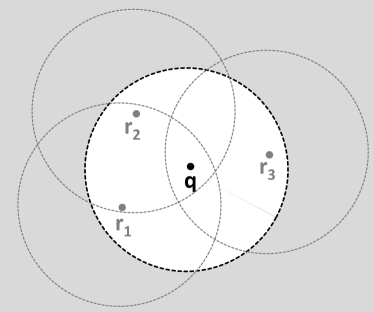
(a) Single query case.

(b) Multiple query case.

Figure 2: Pruning space for $I\varepsilon\mbox{-}RQ$.

4.1 Framework Implementation

Fast Query Based Validation

There is no possible result if there exists a pair $q,q^{\prime}$ of queries in $Q$, such that their $\varepsilon$-ranges do not intersect (i.e., $d(q,q^{\prime})>2\cdot\varepsilon$). In this case, there can be no object $r$ having both $q$ and $q^{\prime}$ within its $\varepsilon$-range (a necessary condition for $r$ to be in the result).

Query Based Pruning

Let $S_{i}^{\varepsilon}\subseteq\mathbb{R}^{d}$ be the $\varepsilon$-sphere around query point $q_{i}$ for all $q_{i}\in Q$, as depicted in the example shown in Figure 2(b). Obviously, any point in the intersection region of all spheres, i.e. $\cap_{i=1..m}S_{i}^{\varepsilon}$, has all query objects $q_{i}\in Q$ in its $\varepsilon$-range. Consequently, all objects outside of this region can be pruned. However, the computation of the search region can become too expensive in an arbitrary high dimensional space; thus, we compute the intersection between rectangles that minimally bound the hyper-spheres and use it as a filter. This can be done quite efficiently even in high dimensional spaces; the resulting filter rectangle is used as a window query and all objects in it are passed to the refinement step as candidates.

Object Based Pruning

As mentioned in Section 3 this filter is not applicable for inverse $\varepsilon$-range queries, since objects cannot be used to prune other objects.

Refinement

In the refinement step, for all candidates we compute their distances to all query points $q\in Q$ and report only objects that are within distance $\varepsilon$ from all query objects.

4.2 Algorithm

The implementation of our framework above can be easily converted to an algorithm, which, after applying the filter steps, performs a window query to retrieve the candidates, which are finally verified. Search can be facilitated by an R-tree that indexes $\mathcal{D}$. Starting from the root, we search the tree, using the filter rectangle. To minimize the I/O cost, for each entry $P$ of the tree that intersects the filter rectangle, we compute its distance to all points in $Q$ and access the corresponding subtree only if all these distances are smaller than $\varepsilon$.

5 Inverse $k$-NN Query

For inverse $k$-nearest neighbor queries (I$k$-NNQ), we first consider the case of a single query object (i.e., $|Q|=1$). As discussed in Section 2, this case can be processed by the bi-section-based R$k$-NN approach (TPL) proposed in [9], enhanced by the rectangle-based pruning criterion proposed in [3]. The core idea of TPL is to use bi-section-hyperplanes between database objects $o$ and the query object $q$ in order to check which objects are closer to $o$ than to $q$. Each bi-section-hyperplane divides the object space into two half-spaces, one containing $q$ and one containing $o$. Any object located in the half-space containing $o$ is closer to $o$ than to $q$. The objects spanning the hyperplanes are collected in an iterative way. Each object $o$ is then checked against the resulting half-spaces that do not contain $q$. As soon as $o$ is inside more than $k$ such half-spaces, it can be pruned. Next, we consider queries with multiple objects (i.e., $|Q|>1$) and discuss how the framework presented in Section 3 is implemented in this case.

5.1 Framework Implementation

Fast Query Based Validation

Recall that this filter uses the set of query objects $Q$ only, to perform a quick check on whether the result is empty. Here, we use the obvious rule that the result is empty if the number of query objects exceeds the query parameter $k$.

Query Based Pruning

We can exploit the query objects in order to reduce the I$k$-NN query to an I$k^{\prime}$-NN query with $k^{\prime}<k$. A smaller query parameter $k^{\prime}$ allows us to terminate the query process earlier and reduce the search space. We first show how $k$ can be reduced by means of the query objects only. The proofs for all lemmas are presented in Appendix 0.A.

Lemma 1

Let $\mathcal{D}\subseteq\mathbb{R}^{d}$ be a set of database objects and $Q\subseteq\mathcal{D}$ be a set of query objects. Let $\mathcal{D}^{\prime}=\mathcal{D}-Q$. For each $o\in\mathcal{D}^{\prime}$, the following statement holds:

$$o\in Ik\mbox{-}NNQ(Q)~{}\textrm{in}~{}\mathcal{D}\Rightarrow\forall q\in Q:o\in Ik^{\prime}\mbox{-}NNQ(\{q\})~{}\textrm{in}~{}\mathcal{D}^{\prime}\cup\{q\},$$

$$\mbox{where }k^{\prime}=k-|Q|+1.$$

Simply speaking, if a candidate object $o$ is not in the $Ik^{\prime}\mbox{-}NNQ(\{q\})$ result of some $q\in Q$ considering only the points $\mathcal{D}^{\prime}\cup\{q\}$, then $o$ cannot be in the $Ik\mbox{-}NNQ(Q)$ result considering all points in $\mathcal{D}$ and $o$ can be pruned. As a consequence, $Ik^{\prime}\mbox{-}NNQ(\{q\})$ in $\mathcal{D}^{\prime}\cup\{q\}$ can be used to prune candidates for any $q\in Q$. The pruning power of $Ik^{\prime}\mbox{-}NNQ(\{q\})$ depends on how $q\in Q$ is selected.

From Lemma 1 we can conclude the following:

Lemma 2

Let $o\in\mathcal{D}-Q$ be a database object and $q_{ref}\in Q$ be a query object such that $\forall q\in Q:d(o,q_{ref})\geq d(o,q)$. Then

$$o\in Ik\mbox{-}NNQ(Q)\Leftrightarrow o\in Ik^{\prime}\mbox{-}NNQ(\{q_{ref}\})~{}\textrm{in}~{}\mathcal{D}^{\prime}\cup\{q\},$$

where $k^{\prime}=k-|Q|+1$.

Lemma 2 suggests that for any candidate object $o$ in $\mathcal{D}$, we should use the furthest query point to check whether $o$ can be pruned.

Object Based Pruning

Up to now, we only used the query points in order to reduce $k$ in the inverse $k$-NN query. Now, we will show how to consider database objects in order to further decrease $k$.

Lemma 3

Let $Q$ be the set of query objects and $\mathcal{H}\subseteq\mathcal{D}-Q$ be the non-query(database) objects covered by the convex hull of $Q$. Furthermore, let $o\in\mathcal{D}$ be a database object and $q_{ref}\in Q$ a query object such that $\forall q\in Q:d(o,q_{ref})\geq d(o,q)$. Then for each object $p\in\mathcal{H}$ it holds that $d(o,p)\leq d(o,q_{ref})$.

According to the above lemma the following statement holds:

Lemma 4

Let $Q$ be the set of query objects, $\mathcal{H}\subseteq\mathcal{D}-Q$ be the database (non-query) objects covered by the convex hull of $Q$ and let $q_{ref}\in Q$ be a query object such that $\forall q\in Q:d(o,q_{ref})\geq d(o,q)$. Then

$$\forall o\in\mathcal{D}-\mathcal{H}-Q:o\in Ik\mbox{-}NNQ(Q)\Leftrightarrow$$

at most $k^{\prime}=k-|\mathcal{H}|-|Q|$ objects $p\in\mathcal{D}-\mathcal{H}$ are closer to $o$ than $q_{ref}$, and

$$\forall o\in\mathcal{H}:o\in Ik\mbox{-}NNQ(Q)\Leftrightarrow$$

at most $k^{\prime}=k-|\mathcal{H}|-|Q|+1$ objects $p\in\mathcal{D}-\mathcal{H}$ are closer to $o$ than $q_{ref}$.

Based on Lemma 4, given the number of objects in the convex hull of $Q$, we can prune objects outside of the hull from I$k$-NN($Q$). Specifically, for an I$k$-NN query we have the following pruning criterion: An object $o\in\mathcal{D}$ can be pruned, as soon as we find more than $k^{\prime}$ objects $p\in\mathcal{D}-\mathcal{H}$ outside of the convex hull of $Q$, that are closer to $o$ than $q_{ref}$. Note that the parameter $k^{\prime}$ is set according to Lemma 4 and depends on whether $o$ is in the convex hull of $Q$ or not. Depending on the size of $Q$ and the number of objects within the convex hull of $Q$, $k^{\prime}=k-|\mathcal{H}|+1$ can become negative. In this case, we can terminate query evaluation immediately, as no object can qualify the inverse query (i.e., the inverse query result is guaranteed to be empty). The case where $k^{\prime}=k-|\mathcal{H}|+1$ becomes zero is another special case, as all objects outside of $\mathcal{H}$ can be pruned. For all objects in the convex hull of $Q$ (including all query objects) we have to check whether there are objects outside of $\mathcal{H}$ that prune them.

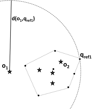
(a) Pruning $o_{1}$

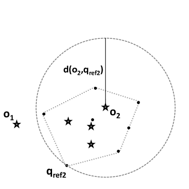
(b) Pruning $o_{2}$

Figure 3: I$k$-NN pruning based on Lemma 4

As an example of how Lemma 4 can be used, consider the data shown in Figure 3 and assume that we wish to perform an inverse 10NN query using a set $Q$ of seven query objects, shown as points in the figure; non-query database points are represented by stars. In Figure 3(a), the goal is to determine whether candidate object $o_{1}$ is a result, i.e., whether $o_{1}$ has all $q\in Q$ in its 10NN set. The query object having the largest distance to $o_{1}$ is $q_{ref1}$. Since $o_{1}$ is located outside of the convex hull of $Q$ (i.e, $o\in\mathcal{D}-\mathcal{H}-Q$), the first equivalence of Lemma 4, states that $o_{1}$ is a result if at most $k^{\prime}=k-|\mathcal{H}|-|Q|=10-4-7=-1$ objects in $\mathcal{D}-\mathcal{H}-Q$ are closer to $o_{1}$ than $q_{ref1}$. Thus, $o_{1}$ can be safely pruned without even considering these objects (since obviously, at least zero objects are closer to $o_{1}$ than $q_{ref1}$). Next, we consider object $o_{2}$ in Figure 3(b). The query object with the largest distance to $o_{2}$ is $q_{ref2}$. Since $o_{2}$ is inside the convex hull of $Q$, the second equivalence of Lemma 4 yields that $o_{2}$ is a result if at most $k^{\prime}=k-|\mathcal{H}|-|Q|+1=10-4-7+1=0$ objects $\mathcal{D}-\mathcal{H}-Q$ are closer to $o_{2}$ than $q_{ref2}$. This, $o_{2}$ remains a candidate until at least one object in $\mathcal{D}-\mathcal{H}-Q$ is found that is closer to $o_{2}$ than $q_{ref2}$.

Refinement

Each remaining candidate is checked whether it is a result of the inverse query by performing a $k$-NN search and verifying whether its result includes $Q$.

5.2 Algorithm

We now present a complete algorithm that traverses an aggregate R-tree ($ARTree$), which indexes $\mathcal{D}$ and computes $Ik\mbox{-}NNQ(Q)$ for a given set $Q$ of query objects, using Lemma 4 to prune the search space. The entries in the tree nodes are augmented with the cardinality of objects in the corresponding sub-tree. These counts can be used to accelerate search, as we will see later.

In a nutshell, the algorithm, while traversing the tree, attempts to prune nodes based on the lemma using the information known so far about the points of $\mathcal{D}$ that are included in the convex hull (filtering). The objects that survive the pruning are inserted in the candidates set. During the refinement step, for each point $c$ in the candidates set, we run a $k$-NN query to verify whether $c$ contains $Q$ in its $k$-NN set.

Algorithm 1 in Appendix 0.B is a pseudocode of our approach. The $ARTree$ is traversed in a best-first search manner [4], prioritizing the access of the nodes according to the maximum possible distance (in case of a non-leaf entry we use MinDist) of their contents to the query points $Q$. In specific, for each R-tree entry $e$ we can compute, based on its MBR, the furthest possible point $q_{ref}$ in $Q$ to a point indexed under $e$. Processing the entries with the smallest such distances first helps to find points in the convex hull of $Q$ earlier, which helps making the pruning bound tighter.

Thus, initially, we set $|\mathcal{H}|=0$, assuming that in the worst case the number of non-query points in the convex hull of $Q$ is 0. If the object which is deheaped is inside the convex hull, we increase $|\mathcal{H}|$ by one. If a non-leaf entry is deheaped and its MBR is contained in the hull, we increase $|\mathcal{H}|$ by the number of objects in the corresponding sub-tree, as indicated by its augmented counter.

During the tree traversal, the accessed tree entries could be in one of the following sets (i) the set of candidates, which contains objects that could possibly be results of the inverse query, (ii) the set of pruned entries, which contains (pruned) entries whose subtrees may not possibly contain inverse query results, and (iii) the set of entries which are currently in the priority queue. When an entry $e$ is deheaped, the algorithm checks whether it can be pruned. For this purpose, it initializes a $prune\_counter$ which is a lower bound of the number of objects that are closer to every point $p$ in $e$ than $Q$’s furthest point to $p$. For every entry $e^{\prime}$ in all three sets (candidates, pruned, and priority queue), we increase the $prune\_counter$ of $e$ by the number of points in $e^{\prime}$ if the following condition holds: $\forall p\in e,\forall p^{\prime}\in e^{\prime}:dist(e,e^{\prime})<dist(e,q_{ref})$. This condition can efficiently be checked using the technique from [3]. An example were this condition is fulfilled is shown in Figure 4. Here the $prune\_counter$ of $e$ can be increased by the number of points in $e^{\prime}$.

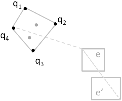
Figure 4: Calculating the $prune\_count$ of e

While updating $prune\_counter$ for $e$, we check whether $prune\_counter>k-|\mathcal{H}|-|Q|$ ($prune\_counter>k-|\mathcal{H}|-|Q|+1$) for entries that are entirely outside of (intersect) the convex hull. As soon as this condition is true, $e$ can be pruned as it cannot contain objects that can participate in the inverse query result (according to Lemma 4). Considering again Figure 4 and assuming the number of points in $e^{\prime}$ to be 5, $e$ could be pruned for $k\leq 10$ (since $prune\_counter(5)>k(10)-|\mathcal{H}|(2)-|Q|(4)$ holds). In this case $e$ is moved to the set of pruned entries. If $e$ survives pruning, the node pointed to by $e$ is visited and its entries are enheaped if $e$ is a non-leaf entry; otherwise $e$ is inserted in the candidates set.

When the queue becomes empty, the filter step of the algorithm completes with a set of candidates. For each object $c$ in this set, we check whether $c$ is a result of the inverse query by performing a $k$-NN search and verifying whether its result includes $Q$. In our implementation, to make this test faster, we replace the $k$-NN search by an aggregate $\varepsilon$-range query around $c$, by setting $\varepsilon=d(c,q_{ref})$, where $q_{ref}$ is the furthest point of $Q$ to $p$. The objective is to count whether the number of objects in the range is greater than $k$. In this case, we can prune $c$, otherwise $c$ is a result of the inverse query. $ARTree$ is used to process the aggregate $\varepsilon$-range query; for every entry $e$ included in the $\varepsilon$-range, we just increase the aggregate count by the augmented counter to $e$ without having to traverse the corresponding subtree. In addition, we perform batch searching for candidates that are close to each other, in order to optimize performance. The details are skipped due to space constraints.

6 Inverse Dynamic Skyline Query

We again first discuss the case of a single query object, which corresponds to the reverse dynamic skyline query [6] and then present a solution for the more interesting case where $|Q|>1$. Let $q$ be the (single) query object with respect to which we want to compute the inverse dynamic skyline. Any object $o\in\mathcal{D}$ defines a pruning region, such that any object $o^{\prime}$ in this region cannot be part of the inverse query result. Formally:

Definition 2 (Pruning Region)

Let $q=(q^{1},\ldots,q^{d})\in Q$ be a single $d$-dimensional query object and $o=(o^{1},\ldots,o^{d})\in\mathcal{D}$ be any $d$-dimensional database object. Then the pruning region $PR_{q}(o)$ of $o$ w.r.t. $q$ is defined as the $d$-dimensional rectangle where the $i$th dimension of $PR_{q}(o)$ is given by $[\frac{q^{i}+o^{i}}{2},+\infty]$ if $q^{i}\leq o^{i}$ and $[-\infty,\frac{q^{i}+o^{i}}{2}]$ if $q^{i}\geq o^{i}$.

The pruning region of an object $o$ with respect to a single query object $q$ is illustrated by the shaded region in Figure 5(a).

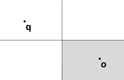
(a) pruning region

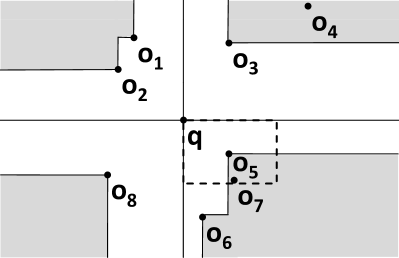
(b) candidates

Figure 5: Single-query case

Filter step. As shown in [6], any object $p\in\mathcal{D}$ can be safely pruned if $p$ is contained in the pruning region of some $o\in\mathcal{D}$ w.r.t. $q$ (i.e. $p\in PR_{q}(o)$). Accordingly, we can use $q$ to divide the space into $2^{d}$ partitions by splitting along each dimension at $q$. Let $o\in\mathcal{D}$ be an object in any partition $P$; $o$ is an $I\mbox{-}DSQ$ candidate, iff there is no other object $p\in P\subseteq\mathcal{D}$ that dominates $o$ w.r.t. $q$.

Thus, we can derive all $I\mbox{-}DSQ$ candidates as follows: First, we split the data space into the $2^{d}$ partitions at the query object $q$ as mentioned above. Then in each partition, we compute the skyline, as illustrated in the example depicted in Figure 5(b). The union of the four skylines is the set of the inverse query candidates (e.g., $\{o_{1},o_{2},o_{3},o_{5},o_{6},o_{8}\}$ in our example).

Refinement. The result of the reverse dynamic skyline query is finally obtained by verifying for each candidate $c$, whether there is an object in $\mathcal{D}$ which dominates $q$ w.r.t. $c$. This can be done by checking whether the hypercube centered at $c$ with extent $2\cdot|c^{i}-q^{i}|$ at each dimension $i$ is empty. For example, candidate $o_{5}$ in Figure 5(b) is not a result, because the corresponding box (denoted by dashed lines) contains $o_{7}$. This means that in both dimensions $o_{7}$ is closer to $o_{5}$ than $q$ is.

6.1 IQ Framework Implementation

Fast Query Based Validation

Following our framework, first the set $Q$ of query objects is used to decide whether it is possible to have any result at all. For this, we use the following lemma:

Lemma 5

Let $q\in Q$ be any query object and let $\mathcal{S}$ be the set of $2^{d}$ partitions derived from dividing the object space at $q$ along the axes into two halves in each dimension. If in each partition $r\in\mathcal{S}$ there is at least one query object $q^{\prime}\in Q$ $(q^{\prime}\neq q)$, then there cannot be any result.

Query Based Pruning

We now propose a filter, which uses the set $Q$ of query objects only in order to reduce the space of candidate results. We explore similar strategies as the fast query based validation. For any pair of query objects $q,q^{\prime}\in Q$, we can define two pruning regions, according to Definition 2: $PR_{q}(q^{\prime})$ and $PR_{q^{\prime}}(q)$. Any object inside these regions cannot be a candidate of the inverse query result because it cannot have both $q_{1}$ and $q_{2}$ in its dynamic skyline point set. Thus, for every pair of query objects, we can determine the corresponding pruning regions and use their union to prune objects or R-tree nodes that are contained in it. Figure 6 shows examples of the pruning space for $|Q|=3$ and $|Q|=4$. Observe that with the increase of $|Q|$ the remaining space, which may contain candidates, becomes very limited.

The main challenge is how to encode and use the pruning space defined by $Q$, as it can be arbitrarily complex in the multidimensional space. As for the $Ik\mbox{-}NNQ$ case, our approach is not to explicitly compute and store the pruning space, but to check on-demand whether each object (or R-tree MBR) can be pruned by one or more query pairs. This has a complexity of $O(|Q|^{2})$ checks per object. In Appendix 0.C, we show how to reduce this complexity for the special 2D case. The techniques shown there can also be used in higher dimensional spaces, with lower pruning effect.

(a) $|Q|=3$

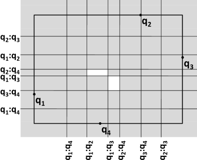
(b) $|Q|=4$

Figure 6: Pruning regions of query objects

Object Based Pruning

For any candidate object $o$ that is not pruned during the query-based filter step, we need to check if there exists any other database object $o^{\prime}$ which dominates some $q\in Q$ with respect to $o$. If we can find such an $o^{\prime}$, then $o$ cannot have $q$ in its dynamic skyline and thus $o$ can be pruned for the candidate list.

Refinement

In the refinement step, each candidate $c$ is verified by performing a dynamic skyline query using $c$ as query point. The result should contain all $q_{i}\in Q$, otherwise $c$ is dropped. The refinement step can be improved by the following observation (cf. Figure 7): for checking if a candidate $o_{1}$ has all $q_{i}\in Q$ in its dynamic skyline, it suffices to check whether there exists at least one other object $o_{j}\in\mathcal{D}$ which prevents one $q_{i}$ from being part of the skyline. Such an object has to lie within the MBR defined by $q_{i}$ and $q_{i}^{\prime}$ (which is obtained by reflecting $q_{i}$ through $o_{1}$). If no point is within the $|Q|$ MBRs, then $o_{1}$ is reported as result.

6.2 Algorithm

The algorithm for $I\mbox{-}DSQ$ is shown as Algorithm 2 in Appendix 0.B. During the filter steps, the tree is traversed in a best first manner, where entries are accessed by their minimal distance (MinDist) to the farthest query object. For each entry $e$ we check if $e$ is completely contained in the union of pruning regions defined by all pairs of queries $(q_{i},q_{j})\in Q$; i.e., $\bigcup_{(q_{i},q_{j})\in Q}PR_{q_{i}}(q_{j})$. In addition, for each accessed database object $o_{i}$ and each query object $q_{j}$, the pruning region is extended by $PR_{q_{j}}(o_{i})$. Analogously to the $Ik\mbox{-}NN$ case, lists for the candidates and pruned entries are maintained. The pruning conditions of Appendix 0.C are used wherever applicable to reduce the computational cost. Finally, the remaining candidates are refined using the refinement strategy described in Section 6.1.

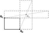
Figure 7: Refinement area defined by $q_{1},q_{2}$ and $o_{1}$

7 Experiments

For each of the inverse query predicates discussed in the paper, we compare our proposed solution based on multi-query-filtering (MQF), with a naive approach (Naive) and another intuitive approach based on single-query-filtering (SQF). The naive algorithm (Naive) computes the corresponding reverse query for every $q\in Q$ and intersects their results iteratively. To be fair, we terminated Naive as soon as the intersection of results obtained so far is empty. SQF performs a R$k$NN (R$\varepsilon$-range / RDS) query using one randomly chosen query point as a filter step to obtain candidates. For each candidate an $\varepsilon$-range ($k$NN / DS) query is issued and the candidate is confirmed if all query points are contained in the result of the query (refinement step). Since the pages accessed by the queries in the refinement step are often redundant, we use a buffer to further boost the performance of SQF. We employed $R^{*}$-trees ([1]) of pagesize 1Kb to index the datasets used in the experiments. For each method, we present the number of page accesses and runtime. To give insights into the impact of the different parameters on the cardinality of the obtained results we also included this number to the charts. In all settings we performed 1000 queries and averaged the results. All methods were implemented in Java 1.6 and tests were run on a dual core (3.0 Ghz) workstation with 2 GB main memory having windows xp as OS. The performance evaluation settings are summarized below; the numbers in bold correspond to the default settings:

parameter	values
db size	100000 (synthetic), 175812 (real)
dimensionality	2, 3, 4, 5
$\varepsilon$	0.04, 0.05, 0.06, 0.07, 0.08, 0.09, 0.1
$k$	50, 100, 150, 200, 250
# inverse queries	1, 3, 5, 10, 15, 20, 25, 30, 35
query extent	0.0001, 0.0002, 0.0003, 0.0004, 0.0005, 0.0006

The experiments were performed using several datasets:

• Synthetic Datasets: Clustered and uniformly distributed objects in $d$-dimensional space.

• Real Dataset: Vertices in the Road Network of North America . Contains 175,812 two-dimensional points.

The datasets were normalized, such that their minimum bounding box is $[0,1]^{d}$. For each experiment, the query objects $Q$ for the inverse query were chosen randomly from the database. Since the number of results highly depends on the distance between inverse query points (in particular for the $I\varepsilon\mbox{-}RQ$ and $Ik\mbox{-}NNQ$) we introduced an additional parameter called extent to control the maximal distance between the query objects. The value of extent corresponds to the volume (fraction of data space) of a cube that minimally bounds all queries. For example in the 3D space the default cube would have a side length of 0.073. A small extent assures that the queries are placed close to each other generally resulting in more results. In this section, we show the behavior of all three algorithms on the uniform datasets only. Experiments on the other datasets can be found in Appendix 0.E.

7.1 Inverse $\varepsilon$-Range Queries

We first compared the algorithms on inverse $\varepsilon$ range queries. Figure 8(a) shows that the relative speed of our approach (MQF) compared to Naive grows significantly with increasing $\varepsilon$; for Naive, the cardinality of the result set returned by each query depends on the space covered by the hypersphere which is in $O(\varepsilon^{d})$. In contrast, our strategy applies spatial pruning early, leading to a low number of page accesses. SQF is faster than Naive, but still needs around twice as much page accesses as MQF. MQF performs even better with an increasing number of query points in $Q$ (as depicted in Figure 8(b)), as in this case the intersection of the ranges becomes smaller. The I/O cost of SQF in this case remains almost constant which is mainly due to the use of the buffer which lowers the page accesses in the refinement step. Similar results can be observed when varying the database size (Figure 8(e)) and query extent (Figure 8(d)). For the data dimensionality experiment (Figure 8(c)) we set epsilon such that the sphere defined by $\varepsilon$ covers always the same percentage of the dataspace, to make sure that we still obtain results when increasing the dimensionality (note, however, that the number of results is still unsteady). Increasing dimensionality has a negative effect on performance. However MQF copes better with data dimensionality than the other approaches. In a last experiment (see Figure 8(f)) we compared the computational costs of the algorithms. Even though Inverse Queries are I/O bound, MQF is still preferable for main-memory problems.

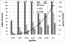
(a) I/O cost w.r.t. $\varepsilon$.

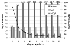
(b) I/O cost w.r.t. $|Q|$.

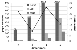
(c) I/O cost w.r.t. $d$.

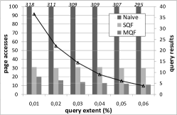
(d) I/O cost w.r.t. extent.

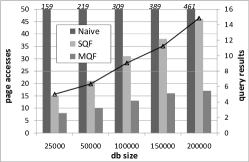
(e) I/O cost w.r.t. $|\mathcal{D}|$.

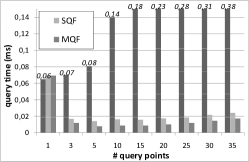
(f) CPU cost w.r.t. $|Q|$.

Figure 8: $I\varepsilon\mbox{-}Q$ algorithms on uniform dataset

7.2 Inverse $k$NN Queries

The three approaches for inverse $k$NN search show a similar behavior as those for the I$\varepsilon$-RQ. Specifically the behavior for varying $k$ (Figure 9(a)) is comparable to varying $\varepsilon$ and increasing the query number (Figure 9(b)) and the query extent (Figure 9(d)) yields the expected results. When testing on datasets with different dimensionality, the advantage of MQF becomes even more significant when $d$ increases (cf. Figure 9(c)). In contrast to the I$\varepsilon$-RQ results for I$k$NN queries the page accesses of MQF decrease (see Figure 9(e)) when the database size increases (while the performance of SQF still degrades). This can be explained by the fact, that the number of pages accessed is strongly correlated with the number of obtained results. Since for the I$\varepsilon$-RQ the parameter $\varepsilon$ remained constant, the number of results increased with a larger database. For I$k$NN the number of results in contrast decreases and so does the number of accessed pages by MQF. As in the previous set of experiments MQF has also the lowest runtime (Figure 9(f)).

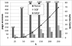
(a) I/O cost w.r.t. $k$.

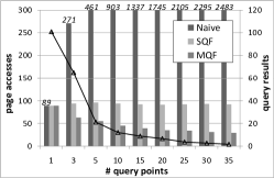
(b) I/O cost w.r.t. $|Q|$.

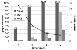
(c) I/O cost w.r.t. $d$.

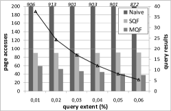
(d) I/O cost w.r.t. extent.

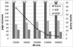
(e) I/O cost w.r.t. $|\mathcal{D}|$.

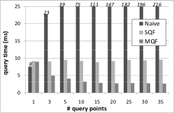
(f) CPU cost w.r.t. $|Q|$.

Figure 9: $Ik\mbox{-}NNQ$ algorithms on uniform dataset

7.3 Inverse Dynamic Skyline Queries

Similar results as for the $Ik\mbox{-}NNQ$ algorithm are obtained for the inverse dynamic skyline queries ($I\mbox{-}DSQ$). Increasing the number of queries in $Q$ reduces the cost of the MQF approach while the costs of the competitors increase. Since the average number of results approaches 0 faster than for the other two types of inverse queries we choose 4 as the default size of the query set. Note that the number of results for $I\mbox{-}DSQ$ intuitively increases exponentially with the dimensionality of the dataset (cf. Figure 10(b)), thus this value can be much larger for higher dimensional datasets. Increasing the distance among the queries does not affect the performance as seen in Figure 10(c); regarding the number of results in contrast to inverse range- and $k$NN-queries, inverse dynamic skyline queries are almost not sensitive to the distance among the query points. The rationale is that dynamic skyline queries can have results which are arbitrary far away from the query point, thus the same holds for the inverse case. The same effect can be seen for increasing database size (cf. Figure 10(d)). The advantage of MQF remains constant over the other two approaches. Like inverse range- and $k$NN-queries, $I\mbox{-}DSQ$ are I/O bound (see Figure 10(e)), but MQF is still preferable for main-memory problems.

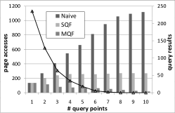
(a) I/O cost w.r.t. $|Q|$.

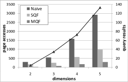
(b) I/O cost w.r.t. $d$.

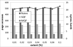
(c) I/O cost w.r.t. extent.

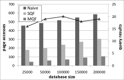
(d) I/O cost w.r.t. $|\mathcal{D}|$.

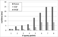
(e) CPU cost w.r.t. $|Q|$.

Figure 10: $I\mbox{-}DSQ$ algorithms on uniform dataset

8 Conclusions

In this paper we introduced and formalized the problem for inverse query processing. We proposed a general framework to such queries using a filter-refinement strategy and applied this framework to the problem of answering inverse $\varepsilon$-range queries, inverse $k$NN queries and inverse dynamic skyline queries. Our experiments show that our framework significantly reduces the cost of inverse queries compared to straightforward approaches. In the future, we plan to extend our framework for inverse queries with different query predicates, such as top-$k$ queries. In addition, we will investigate inverse query processing in the bi-chromatic case, where queries and objects are taken from different datasets. Another interesting extension of inverse queries is to allow the user not only to specify objects that have to be in the result, but also objects that must not be in the result.

Appendix 0.A Proofs of Lemmas

0.A.1 Proof of Lemma 1

Proof

By contradiction: Let $q\in Q$ such that:

$$o\not\in Ik^{\prime}\mbox{-}NNQ(\{q\})~{}\textrm{in}~{}\mathcal{D}^{\prime}\cup\{q\}.$$

That is, $o$ does not have $q$ as one of its $k^{\prime}$-nearest neighbors in the database $\mathcal{D}^{\prime}\cup\{q\}$ containing all (and only) non-query objects and $q$. This implies that there exist at least $k^{\prime}$ objects $o^{\prime}\in\mathcal{D}^{\prime}\cup\{q\}$ such that $dist(o,o^{\prime})<dist(o,q)$. Let $q^{ref}\in Q$ be the query farthest from $o$. Thus, for each of the $Q-1$ objects $q^{\prime}\in Q,q\neq q^{ref}$ it holds that $dist(o,q)<dist(o,q^{ref})$ and for each of the $k^{\prime}$ object $o^{\prime}$ it holds that $dist(o,o^{\prime})<dist(o,q)\leq dist(o,q^{ref})$. Thus there exist at least $Q-1+k^{\prime}=k$ objects that are closer to $o$ than $q^{ref}$. This implies that

$$q^{ref}\not\in kNN(o)~{}\textrm{in}~{}\mathcal{D}$$

and thus

$$o\not\in Ik\mbox{-}NNQ(Q)~{}\textrm{in}~{}\mathcal{D}.$$

Therefore, we have shown that

$$\neg(o\in Ik^{\prime}\mbox{-}NNQ(\{q\})~{}\textrm{in}~{}\mathcal{D}^{\prime}\cup\{q\})\Rightarrow\neg(o\in Ik\mbox{-}NNQ(Q)~{}\textrm{in}~{}\mathcal{D})$$

which is equivalent to

$$o\in Ik\mbox{-}NNQ(Q)~{}\textrm{in}~{}\mathcal{D}\Rightarrow\forall q\in Q:o\in Ik^{\prime}\mbox{-}NNQ(\{q\})~{}\textrm{in}~{}\mathcal{D}^{\prime}\cup\{q\}$$

As a side note: The counter direction $\mathbf{\Leftarrow:}$ also holds, but is not required for pruning.

Proof

Assume that

$$\forall q\in Q:o\in Ik^{\prime}\mbox{-}NNQ(\{q\})~{}\textrm{in}~{}\mathcal{D}^{\prime}\cup\{q\}$$

$$\mbox{where }k^{\prime}=k-|Q|+1.$$

Then, for each $q\in Q$ there exists at most $k^{\prime}-1$ objects $o^{\prime}\in\mathcal{D}\setminus Q$ such that $dist(o,o^{\prime})<dist(o,q)$. In addition, there exist at most $|Q|-1$ query objects $q^{\prime}\in Q\setminus\{q\}$ such that $dist(o,q^{\prime})<dist(o,q)$. Thus, there exist at most $k^{\prime}-1+|Q|-1=k-|Q|+1-1+|Q|-1=k-1$ objects which are closer to $o$ than to $q$, thus $q$ must be a $k$NN of $o$. Since this holds for each $q\in Q$ we get

$$o\in Ik\mbox{-}NNQ(Q)~{}\textrm{in}~{}\mathcal{D}$$

0.A.2 Proof of Lemma 2

Proof

Due to Lemma 1 we have

$$o\in Ik\mbox{-}NNQ(Q)~{}\textrm{in}~{}\mathcal{D}\Rightarrow\forall q\in Q:o\in Ik^{\prime}\mbox{-}NNQ(\{q\})~{}\textrm{in}~{}\mathcal{D}^{\prime}\cup\{q\},$$

Again, let $q^{ref}$ be the query point with the largest distance to $o$. Since $q^{ref}\in Q$ we get:

$$\forall q\in Q:o\in Ik^{\prime}\mbox{-}NNQ(\{q\})~{}\textrm{in}~{}\mathcal{D}^{\prime}\cup\{q\}\Rightarrow$$

$$o\in Ik^{\prime}\mbox{-}NNQ(\{q^{ref}\})~{}\textrm{in}~{}\mathcal{D}^{\prime}\cup\{q^{ref}\}$$

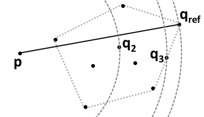
Figure 11: Illustration of Corollary 1

0.A.3 Proof of Lemma 3

We first require the following corollary:

Corollary 1

Let $Q\in\mathbb{R}^{d}$ be a set of points and $Q^{\prime}\subseteq Q$ be the vertices of the convex hull of $Q$ in $\mathbb{R}^{d}$. Then, for each point $o\in\mathbb{R}^{d}$, the farthest point in $Q$ to $o$ must be in $Q^{\prime}$ as well.

Proof

Consider any point $p\in\mathbb{R}^{d}$ and its farthest point $q\in Q$. Then all points in $Q$ must be located in the hyper-sphere centered at $o$ with radius $d(o,q)$. Now, we can proof the above lemma by contradiction assuming that $q$ is not a convex-hull vertex. If $q$ is assumed to be within the convex-hull (not lying on the margin of the convex hull), then the hyper-sphere splits the convex-hull into points that are inside the sphere and points that are out-side of the sphere as shown for $q_{2}$ in Figure 11. Consequently, the convex hull contains points that are farther from $o$ than $q$ which contradicts the assumption. Now, we assume that $q$ lies on the margin (but not on a vertex) of the convex hull which corresponds to a region of a hyper-plane like $q_{3}$ in our example. If we move along this hyper-plane starting from $q$, we are still within the convex-hull but leave the hyper-sphere of $o$. Consequently, again, the convex hull contains points that are farther from $o$ than $q$ which again contradicts the assumption.

Now we can use Corollary 1 to prove Lemma 3:

Proof

By definition of $q_{ref}$ it holds that

$$q_{ref}=argmax_{q\in Q}(dist(o,q))$$

Since the vertices of the convex hull of $Q$ consists only of points in $Q$, Corollary 1 leads to

$$q_{ref}=argmax_{c\in C}(dist(o,c))$$

Thus,

$$\forall c\in C:dist(o,q_{ref})\geq dist(o,c)$$

and since $\mathcal{H}\subseteq C$:

$$\forall p\in\mathcal{H}:dist(o,q_{ref})\geq dist(o,p)$$

0.A.4 Proof of Lemma 4

Proof

$\mathbf{\Rightarrow:}$ If $o\in Ik\mbox{-}NNQ(Q)$, then all query points (including $q_{ref}$) are in the $k$NN set of $o$. Since for all points $p$ in $\mathcal{H}$, $d(o,p)\leq d(o,q_{ref})$ (see Lemma 3), all points in $\mathcal{H}$ should also be in the $k$NN set of $o$. Therefore, in the (worst) case, where $q_{ref}$ is the $k$-th NN of $o$, there can be $k-|\mathcal{H}|-|Q|$ points outside the convex hull closer to $o$ than $q_{ref}$, if $o\notin\mathcal{H}$, or $k-|\mathcal{H}|+1-|Q|$ points if $o\in\mathcal{H}$.

$\mathbf{\Leftarrow:}$ If $o$ is outside the hull, from the points in $\mathcal{H}\cup Q$, $q_{ref}$ is the furthest one to $o$ (see Lemma 3). If there are at most $k-|\mathcal{H}|-|Q|$ points outside the hull closer to $o$ than $q_{ref}$ is, then the distance ranking of $q_{ref}$ is at most $k$. Since all other points in $Q$ are closer to $o$ than $q_{ref}$ is, it should be $o\in Ik\mbox{-}NNQ(Q)$. If $o\in\mathcal{H}$, the bound should be $k-|\mathcal{H}|-|Q|+1$, as $o$ should be excluded from $\mathcal{H}$ in the proof.

0.A.5 Proof of Lemma 5

Proof

Let us consider the space partitioning $\mathcal{S}$ derived from dividing the object space at $q$. Each $q^{\prime}$ located within partition $r\in\mathcal{S}$ generates a pruning region $PR_{q}(q^{\prime})$ (cf. Definition 2) that totally covers the partition $r^{\prime}\in\mathcal{S}$ which is opposite to $r$ w.r.t. $q$. Since we assume that we have at least one query object $q^{\prime}\neq q$ in each partition $r\in\mathcal{S}$, all partitions $r^{\prime}\in\mathcal{S}$ are totally covered by a pruning region and, consequently, the complete data space can be pruned. An example in the two-dimensional space is illustrated in Figure 12.

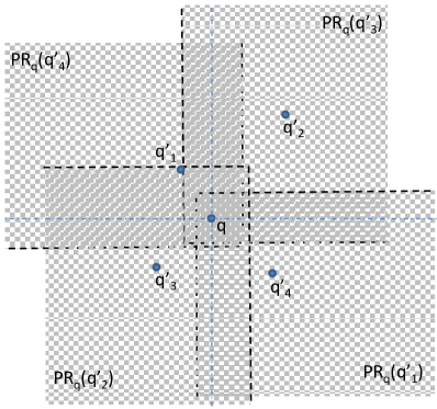
Figure 12: Fast query based validation filter in 2D-space

Appendix 0.B Algorithms

In this section we illustrate the pseudo code of the I$k$NNQ (cf. Algorithm 1) and the IDSQ (cf. Algorithm 2) algorithm. A more detailed explanation is given in Section 5.2 and 6.2 respectively.

Algorithm 1 Inverse kNNQuery

0:  $Q$, $k$, $ARTree$

1:  //Fast Query Based Validation

2:  if $|Q|>k$ then

3:     return ”no result” and terminate algorithm

4:  end if

5:  $pq$ PriorityQueue ordered by $max_{q_{i}\in Q}$MinDist

6:  $pq.add(ARTree.root~{}\textrm{entries})$

7:  $|\mathcal{H}|=0$

8:  LIST $candidates,prunedEntries$

9:  //Query/Object Based Pruning

10:  while $\neg pq.isEmpty()$ do

11:     $e=pq.poll()$

12:     if $getPruneCount(e,Q,candidates,prunedEntries,pq)>k-|\mathcal{H}|-|Q|$ then

13:        $prunedEntries.add(e)$

14:     else if $e.isLeafEntry()$ then

15:        $candidates.add(e)$

16:     else

17:        $pq.add(e.getChildren())$

18:     end if

19:     if $e\in convexHull(Q)$ then

20:        $|\mathcal{H}|+=e.agg\_count$

21:     end if

22:  end while

23:  //Refinement Step

24:  LIST $result$

25:  for  $c\in candidates$ do

26:     if $q_{ref}\in knnQuery(c,k)$ then

27:        $result.add(c)$

28:     end if

29:  end for

30:  return ($result$)

Algorithm 2 Inverse Dynamic Skyline Query

0:  $Q$, $ARTree$

1:  $pq$ PriorityQueue ordered by $min_{q_{i}\in Q}MaxDist$

2:  $pq.add(ARTree.root~{}\textrm{entries})$

3:  LIST $candidates,prunedEntries$

4:  //Filter step

5:  while $\neg pq.isEmpty()$ do

6:     $e=pq.poll()$

7:     if $canBePruned(e,Q,candidates,prunedEntries,pq)$ then

8:        $prunedEntries.add(e)$

9:     else if $e.isLeafEntry()$ then

10:        $candidates.add(e)$

11:     else

12:        $pq.add(e.getChildren())$

13:     end if

14:  end while

15:  //Refinement Step

16:  LIST $result$

17:  for  $c\in candidates$ do

18:     if $Q\in dynamicSkyline(c)$ then

19:        $result.add(c)$

20:     end if

21:  end for

22:  return ($result$)

Appendix 0.C Pruning Candidates in Inverse Dynamic Skyline Queries

Here, we show how pruning a data object from the candidates set of an inverse skyline query can be accelerated. The pruning conditions discussed here hold for the special 2D case. Nonetheless some of them can be extended to spaces of higher dimensionality, with lower pruning effectiveness.

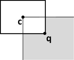
(a) corner point

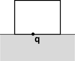
(b) edge point

Figure 13: Using query points at the border of $Q^{\Box}$to prune space

0.C.1 Query-Based Pruning

Let $Q^{\Box}$be the rectangle that minimally bounds all query objects. The main idea is to identify pruning regions by just considering $Q^{\Box}$and one query object $q$ located on the boundary of $Q^{\Box}$. We first concentrate on pruning objects outside $Q^{\Box}$, the cases for pruning objects inside of $Q^{\Box}$will be discussed later.

Pruning Condition I: Assume that $q$ is located at one corner of $Q^{\Box}$, then the axis-aligned region outside of $Q^{\Box}$where the $i$th dimension is defined by the interval $[c^{i},+\infty]$ if $q^{i}>c^{i}$ and $[-\infty,c^{i}]$ otherwise (where $c$ is the center of $Q^{\Box}$) can be pruned. The rationale is that since $Q^{\Box}$is an MBR, at least one other query object must be at each edge of $Q^{\Box}$located on the opposite side of $q$ which can be used to create a pruning region at the side of $q$. In the example shown in Figure 13(a), $q$ is located at the lower right corner of $Q^{\Box}$and, therefore, additional query objects must be located on both the left and upper edge of $Q^{\Box}$. As a consequence, any object in the lower-right shaded region can be pruned.

Pruning Condition II: In the case, where $q$ is located at a boundary of $Q^{\Box}$, but not at a corner of $Q^{\Box}$, the half-space constructed by splitting the data space along the edge containing $q$ and does not contain $Q^{\Box}$defines the pruning region. Here, the rationale is that since $q$ is on an edge $e$ (but not at a corner) of $Q^{\Box}$, there must be at least two additional query objects, located at the edges adjacent to $e$, respectively. By pairing $q$ with each of these two objects, and merging the corresponding pruning regions, we obtain the pruning region. For example, in Figure 13(b), for $q$, we get the shaded pruning region below $q$. As another example, consider the union of $PQ_{q_{1}}(q_{4})$ and $PQ_{q_{3}}(q_{4})$ in Figure 6(b) which prunes the whole hyperplane below $q_{4}$. Thus, if all four edges of $Q^{\Box}$contain four different query objects, then only objects in $Q^{\Box}$are candidate $I\mbox{-}DSQ$ results.

0.C.2 Object-Based Pruning

For any candidate object $o$ that is not pruned during the query-based filter step, we need to check if there exists any other database object $o^{\prime}$ which dominates some $q\in Q$ with respect to $o$. If we can find such an $o^{\prime}$, then $o$ cannot have $q$ in its dynamic skyline and thus $o$ can be pruned for the candidate list. Naively, we can determine, for each database object $o^{\prime}$ that we have found so far and each query object $q$, the pruning region $PR_{q}(o^{\prime})$ according to Definition 2 and check, if $o$ is located in this region. In the following, we show how to perform this pruning without considering all possible combinations of database and query objects.

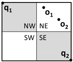
(a) Case 1

(b) Case 2

Figure 14: Object based pruning inside $Q^{\Box}$

Consider two query points $q_{1}$ and $q_{2}$ and the rectangle $Q^{\Box}_{q_{1}q_{2}}$ that minimally bounds $q_{1}$ and $q_{2}$. Note, that $Q^{\Box}_{q_{1}q_{2}}$ is fully contained in $Q^{\Box}$and the union of all $Q^{\Box}_{q_{i}q_{j}}$ for each pair $q_{i},q_{j}\in Q,i\neq j$ is equal to $Q^{\Box}$. Consider the axis-aligned space partitioning according to the center point $c$ of $Q^{\Box}_{q_{1}q_{2}}$ resulting into four partitions, denoted as NE, SE, SW and NW as illustrated in Figure 14. According to the query-based pruning, the two partitions containing $q_{1}$ and $q_{2}$ respectively, can be pruned. Now, we can show the following:

Corollary 2

In each of the two remaining regions (NE and SW in the example) within $Q^{\Box}_{q_{1}q_{2}}$, there can only be at most one candidate.

To prove this, let us consider the following two cases illustrated in Figures 14(a) and 14(b):

Case 1: Let us assume that there are two objects $o_{1}$ and $o_{2}$ in one of the regions, that have the same topology as the two query objects $q_{1}$ and $q_{2}$, as shown in Figure 14(a). In this case both objects prune each other. The reason is that $o_{1}$ is in the pruning region of $o_{2}$ w.r.t. $q_{2}$ and $o_{2}$ is in the pruning region of $o_{1}$ w.r.t. $q_{1}$. Consequently, there cannot exist two candidates in this partition where the objects have similar spatial relationship as $q_{1}$ and $q_{2}$.

Case 2: Now, we assume that there exist two objects $o_{1}$ and $o_{2}$ in one partition within $Q^{\Box}_{q_{1}q_{2}}$ such that $o_{1}o_{2}$ is orienter perpendicularly to $q_{1}q_{2}$, as illustrated in the example in Figure 6(b). In this case, $o_{1}$ is pruned by $o_{2}$ for both query objects. The reason is that in each dimension, the distance between $o_{1}$ and $o_{2}$ must be less than the distance between $o_{1}$ and $q_{1}$ ($q_{2}$). However, $o_{2}$ can in general not be pruned by $o_{1}$, thus $o_{2}$ remains a candidate.

We can now use Corollary 2 to obtain the following pruning condition:

Pruning Condition III: Let $R\subseteq Q^{\Box}$ be a region inside the query rectangle that cannot be pruned using query-based pruning. Let $q_{1},q_{2}\in Q$ be two query points for which it holds that $R$ is fully contained in the rectangle minimally bounding $q_{1}$ and $q_{2}$. Since $R$ cannot be pruned based on query-pruning only, $R$ must be located in non-pruning regions (e.g. NE and SW in Figure 6(a)) of $q_{1}$ and $q_{2}$. Without loss of generality, let us assume that $R$ is located in the NE region of $Q^{\Box}_{q_{1}q_{2}}$. Now Let $O$ be the set of database objects inside $R$. Let $a\in O$ be the object with the largest $x$ coordinate and let $b\in O$ be the object with the largest $y$ coordinate. If $a\neq b$ we can prune $R$. If $a=b$, then $a$ is a candidate and all other objects $c\in R,c\neq a$ can be pruned.

The above pruning condition allows us to prune objects inside $Q^{\Box}$. The next pruning condition allows us to prune objects outside $Q^{\Box}$using database objects. In the following, let $Q^{\Box}_{i}.max$ and $Q^{\Box}_{i}.min$ denote the maximal and minimal coordinate of $Q^{\Box}$, at dimension $i$, respectively.

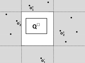
Figure 15: Pruning regions outside of $Q^{\Box}$.

Pruning Condition IV: For the next pruning condition we use the sets of database objects $O_{i}\subseteq\mathcal{D}$ outside $Q^{\Box}$for which it holds that each $o\in O_{i}$ intersects $Q^{\Box}$in one dimension but not in the other. Such objects are shown in Figure 15. Let $O^{+}_{i}$ ($O^{-}_{i}$) denote the subset of $O_{i}$ so that each object $o\in O^{+}_{i}$ has a larger (smaller) coordinate than $Q^{\Box}$ in the other dimension. Now let $o^{+}_{i}\in O^{+}_{i}$ ($o^{-}_{i}\in O^{-}_{i}$) be the object in $O^{+}_{i}$ ($O^{-}_{i}$) with the smallest (largest) coordinate in the other dimension $j$. Any database object which has a $j$ coordinate greater than $\frac{o^{+}_{i}+Q^{\Box}_{i}.max}{2}$ or less than $\frac{o^{-}_{i}+Q^{\Box}_{i}.min}{2}$ can be pruned. The rationale of this pruning condition is that due the MBR property of $Q^{\Box}$, we know that at least one query object must be located on each edge of $Q^{\Box}$. The pruning regions defined are based on these query objects. For instance, for object $o_{1}^{+}$ in Figure 15 we can exploit that there must be query objects $q_{1}$ and $q_{2}$ located on the left and the right border edge of $Q^{\Box}$, respectively. This allows us to create the two pruning regions $PR_{q_{1}}(o_{1}^{+})$ and $PR_{q_{2}}(o_{1}^{+})$ according to Definition 2. These pruning regions are smallest, if $q_{1}$ and $q_{2}$ are located at the upper corners of $Q^{\Box}$. Thus, we can prune any object above the line biscecting the upper side of $Q^{\Box}$ and $o_{1}^{+}$.

Appendix 0.D Pruning Techniques For The Bi-Chromatic Case

Here, we explain how the proposed pruning techniques which are designed for the mono-chromatic case can easily be adapted to the bi-chromatic case. Here we assume two data sets $\mathcal{D}$ and $\mathcal{D}^{\prime}$. A bi-chromatic inverse query returns the set of objects $r\in\mathcal{D}^{\prime}$ for which each inverse query object $q\in Q\subseteq\mathcal{D}^{\prime}-$ is contained in the result of a $\mathcal{P}$ query applied on data set $\mathcal{D}$ using $r$ as query object. For each case of the predicate $\mathcal{P}$, we briefly explain the changes to our technique.

Bi-Chromatic I$\varepsilon$-Range Queries

Here, the filter rectangle can directly be applied to $\mathcal{D}^{\prime}$, so there is no practical change.

Bi-Chromatic IkNN Queries

In this case we have to avoid allowing objects in $\mathcal{D}^{\prime}$ to prune each other. In contrast to the mono-chromatic case, we only have to consider objects in $\mathcal{D}$ to build $H$, i.e. the number of objects in the convex hull regions of $Q$.

Bi-Chromatic Inverse Dynamic Skyline Queries

In this case, the pruning region is only defined by objects in $\mathcal{D}$. This pruning region is used to prune objects in $\mathcal{D}^{\prime}$.

Appendix 0.E Additional Experiments

In this section we show the behavior of inverse queries on other datasets than the ones used in section 7. We excluded from the evaluation the Naive approach due to its poor performance; this way, the difference between MQF and SQF becomes more clear. Due to space limitations we focused on I$k$NN queries on the clustered dataset (cf. Figure 16) and the real dataset (cf. Figure 17). Let us note that similar trends could be observed for the other inverese query types.

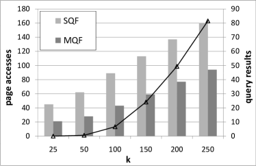
(a) I/O cost w.r.t. $k$.

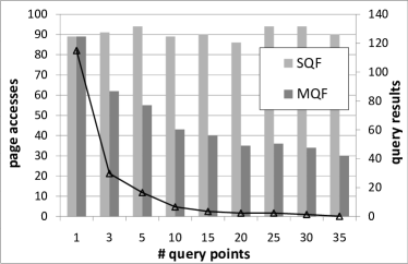
(b) I/O w.r.t. $|Q|$.

(c) I/O w.r.t. $d$.

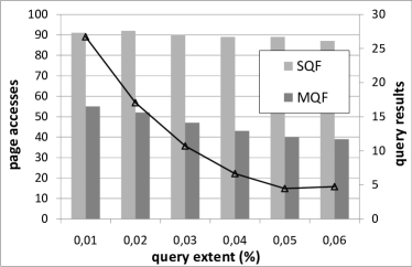
(d) I/O w.r.t. extent.

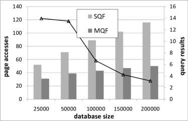
(e) I/O w.r.t. $|\mathcal{D}|$.

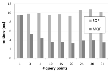
(f) CPU w.r.t. $|Q|$.

Figure 16: $Ik\mbox{-}NNQ$ algorithms on clustered dataset

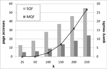
(a) I/O cost w.r.t. $k$.

(b) I/O w.r.t. $|Q|$.

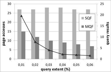
(c) I/O w.r.t. extent.

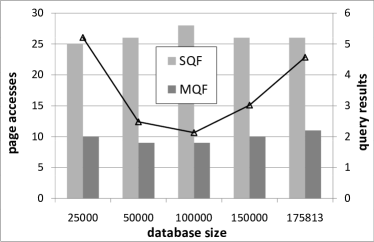
(d) I/O w.r.t. $|\mathcal{D}|$.

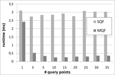
(e) CPU cost w.r.t. $|Q|$.

Figure 17: $Ik\mbox{-}NNQ$ algorithms on real dataset

References

- [1] N. Beckmann, H.-P. Kriegel, R. Schneider, and B. Seeger. The R*-Tree: An efficient and robust access method for points and rectangles. In Proc. SIGMOD, 1990.
- [2] E. Dellis and B. Seeger. Efficient computation of reverse skyline queries. In VLDB, pages 291–302, 2007.
- [3] T. Emrich, H.-P. Kriegel, P. Kröger, M. Renz, and A. Züfle. Boosting spatial pruning: On optimal pruning of mbrs. In SIGMOD, June 6-11, 2010.
- [4] G. R. Hjaltason and H. Samet. Ranking in spatial databases. In Proc. SSD, 1995.
- [5] F. Korn and S. Muthukrishnan. Influence sets based on reverse nearest neighbor queries. In Proc. SIGMOD, 2000.
- [6] X. Lian and L. Chen. Monochromatic and bichromatic reverse skyline search over uncertain databases. In SIGMOD Conference, pages 213–226, 2008.
- [7] A. Singh, H. Ferhatosmanoglu, and A. S. Tosun. High dimensional reverse nearest neighbor queries. In Proc. CIKM, 2003.
- [8] I. Stanoi, D. Agrawal, and A. E. Abbadi. Reverse nearest neighbor queries for dynamic databases. In Proc. DMKD, 2000.
- [9] Y. Tao, D. Papadias, and X. Lian. Reverse kNN search in arbitrary dimensionality. In Proc. VLDB, 2004.
- [10] A. Vlachou, C. Doulkeridis, Y. Kotidis, and K. Nørvåg. Reverse top-k queries. In ICDE, pages 365–376, 2010.
- [11] C. Yang and K.-I. Lin. An index structure for efficient reverse nearest neighbor queries. In Proc. ICDE, 2001.