From 3D to 2D Hydrodynamics in Interacting Micro-rods

Abstract

Moving micron scale objects are strongly coupled to each other by hydrodynamic interactions. The strength of this coupling decays as the inverse particle separation when the two objects are sufficiently far apart. It has been recently demonstrated that the reduced dimensionality of thin fluid layer gives rise to longer ranged, logarithmic coupling. Using holographic tweezers we show that microrods display both behaviors interacting like point particle in 3D at large distance and like point particles in 2D for distances shorter then their length. We derive a simple analytical expression that fits remarkably well our data and further validate it with finite element analysis.

Flagella, microtubules, nanotubes and nanowires are a few examples of the rich variety of fundamental roles that slender bodies have in physics, chemistry and biology. They all share the same geometrical feature of being “slender”, that is having a linear dimension which is much larger than the other two. As a consequence of that they’re all expected to have a similar physical behavior in those situations where only shape matters. That is, for example, the case for micro-hydrodynamics. A thin nanotube or a thicker microrod will both experience a similar drag force, which will depend mainly on the body length while thickness only appears in logarithmic terms happel . While there’s a huge amount of work on single slender body dynamics, especially in the context of bacterial motility lighthill , investigation of hydrodynamic interactions between slender bodies is almost only limited to the phenomenology of syncronization reich ; polin . One reason could be that, as opposed to spheres, which have been studied extensively crocker ; meiners ; ring , hydrodynamic couplings between anisotropic bodies are a complex function of both relative distance and orientation. Optical tweezers can be used to trap and move one dimensional objects tan ; onofrio ; marago . In particular, holographic optical trapping has been shown to be an ideal tool for full 3D micromanipulation of microrods and nanotubes plewa ; grier ; simpson ; ikin ; carberry . Such capabilities offer a unique opportunity for trapping and orienting slender bodies in well defined relative configuration, and directly probe their coupled Brownian dynamics.

In this Letter we provide a direct measurement of hydrodynamic coupling between a pair of parallel aligned silica microrods optically trapped in blinking holographic tweezers. We found a crossover from 3D behavior at large distances, to a 2D logarithmic behavior, when the distance falls below the rods length. Experimental data are in excellent agreement with finite element analysis and can be very well reproduced by a simplified theoretical approach.

In a practically zero Reynolds number regime, as it is in the mesoscopic world, a moving objects generates a perturbation in the surrounding fluid that decays as the inverse distance happel ; Kim . A nearby particle will be transported by this flow and experience a higher mobility when trying to move along the same direction of the other particle. For the same reasons relative motions are characterized by lower mobilities. For well separated objects, collective and relative mobilities can be easily derived assuming that each object is rigidly transported by the approximately uniform flow field produced by the other one. Within this approximation when forces $\mathbf{F}_{1}$ and $\mathbf{F}_{2}$ are applied to two bodies they will move with speeds:

$$\begin{array}[]{rcl}\mathbf{U}_{1}&=&\mathbf{M}_{1}\cdot\mathbf{F}_{1}+\mathbf{u}_{12}\\ \mathbf{U}_{2}&=&\mathbf{M}_{2}\cdot\mathbf{F}_{2}+\mathbf{u}_{21}\end{array}$$ (1)

where $\mathbf{M}_{i}$ is the ith body mobility tensor while $\mathbf{u}_{ij}$ represents the flow that object $j$ produces at the location of $i$. Due to linearity in Stokes flow, flow fields have the form:

$$\mathbf{u}_{ij}=\mathbf{G}_{ij}\cdot\mathbf{F}_{j}$$ (2)

the flow propagator $\mathbf{G}_{ij}$ will depend on distance and on the relative orientation of particle $j$. Introducing the velocity and force vectors $\mathds{U}=\left(\mathbf{U}_{1},\mathbf{U}_{2},\dots\right)$ and $\mathds{F}=\left(\mathbf{F}_{1},\mathbf{F}_{2},\dots\right)$, the full many-body problem can be then stated in the form of a compact mobility matrix formulation:

$$\mathds{U}=\mathds{M}\cdot\mathds{F}$$ (3)

where $\mathds{M}$ is the mobility matrix:

$$\mathds{M}=\left(\begin{array}[]{ccc}\mathbf{M}_{1}&\mathbf{G}_{12}&\dots\\ \mathbf{G}_{21}&\mathbf{M}_{2}&\dots\\ \vdots&\vdots&\ddots\\ \end{array}\right)$$ (4)

with hydrodynamic couplings appearing as off-diagonal terms. At large enough distances, whatever is the shape of $j$, the propagator will tend to to the Oseen tensor that only depends on the position vector $\mathbf{r}_{ij}=\mathbf{r}_{i}-\mathbf{r}_{j}$:

$$\mathbf{G}_{O}(\mathbf{r}_{ij})=\frac{1}{8\pi\mu\;r_{ij}}\left(\mathds{1}+\hat{\mathbf{r}}_{ij}\hat{\mathbf{r}}_{ij}\right)$$ (5)

The Oseen tensor represents the first term in the multipole expansion of the Stokes flow produced by a given force spatial distribution, also known as the Stokeslet. The Stokeslet propagates the perturbation of a zero-dimensional point force and therefore does not depend on particle shape and orientation. For spherical beads it provides a remarkably good description of couplings down to interparticle distances of about 2.5 radii crocker ; meiners ; ring . For anisotropic bodies, higher order terms will have to be included and their form will depend on particle shape and orientation. A thin rod may be thought as the simplest anisotropic body consisting of a one dimensional line force distribution. Most of the shape dependence occurs via a single parameter, that is the body length $L$, and rod orientation matters. Such a dependence on orientations, coupled to the long range character of Stokes propagators, makes hydrodynamic coupling between thin rods a very challenging problem both from the experimental and theoretical point of view. As a first starting approach we could limit ourselves to a single pair of interacting rods at a fixed distance. Slender body theory provides a practical theoretical framework for unidimensional objects where the point force description of the sphere is substituted by a line distribution of point forces. Slender body theory has been successfully applied in the context of flagellar and ciliar propulsion in bacteria. We have seen that coupling terms in the mobility matrix can be thought, as a first approximation, as the flow propagators between interacting objects. Although this is straightforward in the case of spheres, where sphere’s center is a good representative point of sphere position and center of forces, it is quite ambiguous when bodies of extended size are considered. It can be shown Kim that when a thin prolate spheroid is immersed in an external inhomogeneous flow, it will move with a speed given by the average of the original flow over the rod’s length. This finding suggests that we can approximate the hydrodynamic coupling between the rods as the average flow produced by one rod over the length of the other one. For parallel aligned rods like in Fig. 1 this amounts to the double Stokeslet integration:

$$G^{xx}(d)=\int_{-L/2}^{L/2}\!\!\!dy_{2}\int_{-L/2}^{L/2}\!\!dy_{1}\frac{1}{8\pi\mu}\left(\frac{1}{\sqrt{d^{2}+(y_{2}-y_{1})^{2}}}+\frac{d^{2}}{d^{2}+(y_{2}-y_{1})^{2}}\right)=\frac{1}{8\pi\mu L}\log\left[\frac{L+\sqrt{L^{2}+d^{2}}}{\sqrt{2L^{2}+d^{2}-2L\sqrt{L^{2}+d^{2}}}}\right]$$ (6)

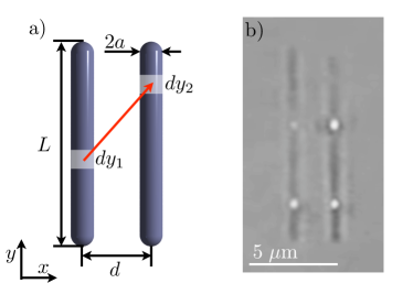
Figure 1: a) Geometrical parameters of the investigated microrods configurations. b) Two silica microrods, each one held in a double holographic trap.

When the two rods are much far apart than their length, the obtained propagator reduces obviously to the Oseen tensor component:

$$G^{xx}(d\gg L)\simeq\frac{1}{4\pi\mu d}.$$ (7)

More interestingly, for separations that are much smaller than rods length, the propagator has the logarithmic expression:

$$G^{xx}(d\ll L)\simeq\frac{1}{4\pi\mu L}\log\frac{2L}{d}$$ (8)

Such a form reminds very closely of what is observed for hydrodynamic coupling in two dimensional thin liquid layers 2d . In other words, microrods interact like point particles in 3D when they are very far away, and then like point particles in 2D at short distances. The crossover distance is determined by the most important length in the problem, that is the rod’s length. Such a finding is not surprising when one realizes that at short distances the problem reduces to the idealized two dimensional case of infinitely long cylinders, where the finite length of the two rods is only responsible for edge effects. Our simple formula seems to provide a good interpolation between the two limiting cases but too crude approximations might be involved in its derivation and we decided to test it against finite element analysis. The model consists of two cylinders of length $L$ and radius $a$ at distance $d$. Finite size effects are reduced by having the two cylinders inside a fluid sphere of radius $100L$. No-slip boundary conditions are set on the cylinder surfaces. We then calculate Stokes drag on the cylinders in the case of rigid and relative motion at different $d$ values. Hydrodynamic coupling is then obtained as half the difference between rigid and relative mobilities. The resulting values for coupling $G^{xx}$ are reported as solid circles in Fig. 2 showing a remarkable good agreement with the analytical expression in (6) also plotted as a solid line.

The chance of observing two rods, occasionally aligned in parallel at some given distance, clearly makes the problem practically impossible to approach experimentally by simple video microscopy observations. However holographic tweezers provide an ideal tool to directly verify our results by trapping and orienting two slender objects in well defined and reproducible relative configurations. We used holographic tweezers to manipulate silica microrods of about 10 $\mu$m in length and 150 nm in radius carberry . Multiple optical traps are obtained by shaping an expanded CW laser beam (532 nm) with a spatial light modulator (Holoeye LC-R 2500). The shaped beam is then focused by a microscope objective of high numerical aperture (Nikon Plan Apo 100x, NA 1.4) onto the target array of trapping spots. Optimal intensity distribution are generated by GSW algorithm running on an NVIDIA GPU (GTX 480) gsw ; cuda . Each rod is held in two traps independently and dynamically reconfigurable (Fig. 1b). The two rods can be aligned and moved at different distances. We limit ourselves to the computed case of center of mass dynamics of parallel aligned rods. Using a chopper on the trapping beam, we periodically release the rods every 1/15 s and subsequently start recording bright field images at 300 fps for 1/30 s. The horizontal $x$ coordinate of each rod is tracked by fitting the row average intensity profile of cropped rods images. A straightforward way to obtain hydrodynamic couplings is that of tracking rods free Brownian motion. We have estimated and experimentally verified that our rods have a rotational diffusion coefficient of about 0.02 rad²/s. That means that the mean squared angular displacement during acquisition time is about $\pi$/100. It is therefore safe to neglect rotational-translational coupling doi ; yodh and project on the $x$ axis the mobility problem with stochastic forces:

$$\begin{array}[]{c}\left(\begin{array}[]{c}\dot{x}_{1}(t)\\ \dot{x}_{2}(t)\end{array}\right)=\mathds{M}^{xx}\cdot\left(\begin{array}[]{c}\eta_{1}(t)\\ \eta_{2}(t)\end{array}\right)\\[14.22636pt] \mathds{M}^{xx}=\left(\begin{array}[]{cc}m_{1}&G^{xx}(d)\\ G^{xx}(d)&m_{2}\end{array}\right)\end{array}$$ (9)

where $m_{1}$ and $m_{2}$ are the transverse mobilities of the two rods while $\eta_{1}$ and $\eta_{2}$ are stochastic forces with zero average and correlation:

$$\langle\eta_{i}(0)\eta_{j}(t)\rangle=2k_{B}T(\mathds{M}^{xx})^{-1}_{ij}\;\delta(t)$$ (10)

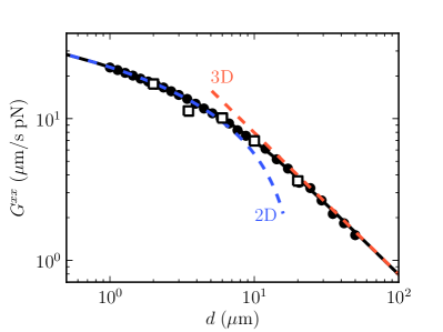
Figure 2: Hydrodynamic coupling $G^{xx}$ between two parallel aligned thin rods as a function of their relative distance. Solid line represents the simple theory in eq. (6). Black circles are numerical results from finite element analysis. Experimental data are reported as open squares. Dashed lines represent the long (7) and short (8) distance limiting behavior reducing to respectively 3D and 2D hydrodynamic couplings between point particles.

This is a coupled Langevin equation leading to a displacements covariance matrix murphy :

$$\begin{array}[]{c}\langle(x_{i}(t)-x_{i}(0))(x_{j}(t)-x_{j}(0))\rangle=2D_{ij}t\\[14.22636pt] D_{ij}=k_{B}T\;\mathds{M}^{xx}_{ij}\end{array}$$ (11)

Diagonal terms represent the mean squared displacements of the two rods. The corresponding diffusion coefficients provide a direct measurement of single particle mobilities. On the other hand hydrodynamic couplings are easily extracted from the diffusion coefficients of the off diagonal terms. In Fig. 3 we report the two single particle mean squared displacements toghether with the crossed term for interparticle distances of 3.5 and 20 microns. Diffusion coefficients can be easily extracted by fitting with a straight line. Single particle diffusion coefficients don’t show a systematic dependence on interparticle distance and their deviations are mainly attributable to small differences in rod lengths. Microrods in our sample have an average length of 10.5 $\mu$m with a standard deviation of 2.5%. Tracking single rod Brownian motion, we extract an average transverse mobility of 42 $\mu$m/s pN. By theoretical predictions, this corresponds to an average rod thickness of about 200 nm, which is well compatible with the nominal pore size (300 nm) used for rod’s growth carberry . Turning now to hydrodynamic couplings, the diffusion coefficient of crossed terms directly provides a measure of $G^{xx}(d)$ through (11). Indeed we found an excellent agreement with theoretical and numerical predictions as shown in Fig. 2. It is worth to note that coupling values are expected to be much less affected by the actual rod thickness than the single rod mobilities, as can be understood noticing that the thickness never entered in the arguments leading to (6). In particular, the results in Fig. 2 are expected to remain valid even in the case of vanishing rods thickness, as could be the case for single walled carbon nanotubes, microtubules or short straight DNA segments.

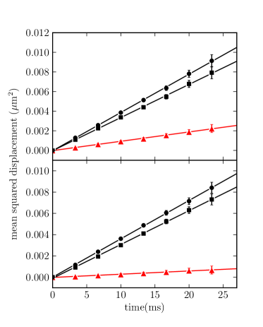
Figure 3: Mean squared displacements of freely diffusing rods starting off a parallel aligned configuration generated with holographic optical tweezers. Top and bottom panel refer respectively to interparticle distances of 3.5 and 20 $\mu$m. Solid circles and squares represent the diagonal terms of the generalized MSD while solid triangles refer to the off diagonal terms. Linear fits are also reported as solid lines.

In conclusion, we have directly measured hydrodynamic interactions between freely diffusing micro-rods. We demonstrated by direct experimental observation and numerical finite element analysis that two parallel aligned microrods interact like point particles in 3D when they’re much farther then their lentgh, and like point particles in 2D for short distances. We also derived a simple analytical expression that reproduces very well both experimental and numerical data. Although the validity of our results is expected to hold even for much thinner, and interesting objects, like nanotubes or microtubules, an experimental investigation of hydrodynamic coupling in those systems remains an open and challenging problem. This work was partially supported by IIT-SEED BACTMOBIL project and MIUR-FIRB project RBFR08WDBE.

References

- (1) J. Happel and H. Brenner, Low Reynolds Number Hydrodynamics, Kluwer Academic, Dordrecht, (1983).
- (2) J. Lighthill, Mathematical Biofluiddynamics, SIAM, Philadelphia (1975).
- (3) M. Reichert and H. Stark, Eur. Phys. J. E 17, 493 (2005).
- (4) M. Polin, I. Tuval, K. Drescher, J.P. Gollub, and R. E. Goldstein, Science 325, 487 (2009).
- (5) J. Crocker, J Chem Phys, 106, 2837 (1997).
- (6) J. Meiners and S. Quake, Phys. Rev. Lett., 82, 2211 (1999).
- (7) R. Di Leonardo, et al., Phys. Rev. E, 76, 258301 (2007).
- (8) S. Tan, H.A. Lopez, C.W. Cai, Y. Zhang, Nano Lett. 4, 1415 (2004)
- (9) O.M. Maragò, et al. Nano Lett., 8, 3211 (2008).
- (10) O.M. Maragò et al. ACS Nano, 4, 7515 (2010).
- (11) J. Plewa, E. Tanner, D. Mueth, D. Grier, Opt. Express 12, 1978 (2004).
- (12) R. Agarwal, K. Ladavac, Y. Roichman, G. H. Yu, C. M. Lieber, and D. G. Grier, Opt. Express 13, 8906 (2005).
- (13) S.H. Simpson and S.Hanna, JOSA A, 27, 1255 (2010).
- (14) L. Ikin, D.M. Carberry, G.M. Gibson, M.J. Padgett, and M.J. Miles, New J. Phys. 11, 023012 (2009).
- (15) D.M. Carberry et al., Nanotechnology, 21, 175501, (2010).
- (16) S. Kim and S. J. Karrila, Microhydrodynamics: princi- ples and selected applications, Dover (2005).
- (17) R. Di Leonardo, S. Keen, F. Ianni, J. Leach, M. Padgett, Ruocco G., Phys. Rev. E, 78, 031406, (2008).
- (18) R. Di Leonardo, F. Ianni, G. Ruocco, Optics Express, 15, 1913, (2007).
- (19) S. Bianchi, R. Di Leonardo, Comp. Phys. Comm., 181, 1444, (2010).
- (20) M. Doi and S.F. Edwards, The theory of polymer dynamics, Oxford University Press, New York (1986).
- (21) Y. Han, A.M. Alsayed, M. Nobili, J. Zhang, T.C. Lubensky, A.G. Yodh, Science, 314, 626 (2006).
- (22) T.J. Murphy and J.L. Aguirre, J. Chem. Phys. 57, 2098 (1972).