Dynamics and Pattern Formation in Large Systems of Spatially-Coupled Oscillators with Finite Response Times

Abstract

We consider systems of many spatially distributed phase oscillators that interact with their neighbors. Each oscillator is allowed to have a different natural frequency, as well as a different response time to the signals it receives from other oscillators in its neighborhood. Using the ansatz of Ott and Antonsen (Ref. OA1 ) and adopting a strategy similar to that employed in the recent work of Laing (Ref. Laing2 ), we reduce the microscopic dynamics of these systems to a macroscopic partial-differential-equation description. Using this macroscopic formulation, we numerically find that finite oscillator response time leads to interesting spatio-temporal dynamical behaviors including propagating fronts, spots, target patterns, chimerae, spiral waves, etc., and we study interactions and evolutionary behaviors of these spatio-temporal patterns.

Many physical systems can be thought of as consisting of a large number of oscillating units that are distributed in space and coupled to neighboring units that are within some limited distance. The individual coupled units of such systems, moreover, can have non-negligible response times, and it is well known that delays can give rise to a set of possible behaviors that is significantly richer than would be the case without delays. Our work addresses two issues: (1) derivation of a macroscopic description for such systems, and (2) the possible characteristic behaviors that may be revealed through study of such macroscopic descriptions.

I Introduction

Systems of large coupled oscillator networks appear in many physical and engineering systems PRK -Winfree . Examples include synchronous flashing of fireflies Buck , pedestrian induced oscillations of the Millennium Bridge MillB , cardiac pace-maker cells Glass , alpha rhythms in the brain Brain , glycolytic oscillations in yeast populations Yeast , cellular clocks governing circadian rhythm in mammals Yamaguchi , oscillatory chemical reactions Kuramoto1 -Taylor , etc.

Many previous studies of oscillator networks developed in the setting of network couplings on graphs with different topological characterizations, such as small-world, Erdös-Renyi, and scale-free (e.g., Refs. Hong -Restrepo ). Here we consider applications in which the oscillators are distributed spatially, for example, when there is a row of trees each occupied with a large number of fireflies. Indeed, in the past decade studies of spatially distributed coupled oscillators have aroused much interest. An example is the chimera states (e.g., Refs. Kura_Batto -Laing2 ), in which there is a stable coexistence of both coherent and incoherent states distributed in space.

Another important aspect of the dynamics of oscillator networks is that physical oscillators may have significant delays in their response to signals and these signals may also take a significant time to propagate. Studies of time-delay effects in the context of all-to-all coupled networks with a homogeneous distribution of time delays (YS , CKK ) show that interesting features such as bistable behaviors and multiple coherent states are induced in the presence of time delays. Reference Lee , building on the machinery developed in Refs. OA1 -OA3 , extends this line of study to a heterogeneous nodal response time distribution. In addition, Ref. Sethia studies the dynamics of a one dimensional ring of spatially distributed and non-locally coupled oscillator network when the time delays are due to signal propagation between interacting oscillators.

The problem studied in this paper is that of uncovering the spatio-temporal dynamics of a system of coupled oscillators with heterogeneous oscillator response times. We first give a microscopic description of the individual oscillators and their couplings. We then spatially coarse-grain this description and use the methods developed in Refs. Laing2 and Lee to derive a set of partial differential equations giving a macroscopic description of the system dynamics. Using our derived macroscopic equations, we then numerically explore the spatio-temporal dynamics and resulting pattern formation in both one- and two-dimensions. We find that a rich variety of behaviors are induced by the presence of time delay in the oscillator response. These include hysteresis, propagating fronts, spots, target patterns, chimerae, spiral waves, etc.

II Formulation

We consider a system of $N$ spatially distributed interacting phase oscillators with time delays between the response of an oscillator and the signal it receives. The evolution equation of oscillator $m$ is

$$\frac{d}{dt}\theta_{m}(t) =\omega_{m}+\sum_{n\neq m}^{N}\hat{K}_{mn}\left\{\sin[\theta_{n}(t-\tau_{mn})-\theta_{m}(t)]\right\}$$

$$=\omega_{m}+\sum_{n\neq m}^{N}\hat{K}_{mn}\frac{1}{2i}\{e^{-i[\theta_{m}(t)-\theta_{n}(t-\tau_{mn})]}-c.c.\},$$ (1)

where $\hat{K}_{mn}$ is the interaction strength between oscillators $m$ and $n$, which is assumed to be spatial in character (i.e., $\hat{K}_{mn}$ becomes small or zero if the distance between oscillator $m$ and oscillator $n$ is large), $\tau_{mn}$ is the interaction time delay in the effect of oscillator $n$ on oscillator $m$, and $c.c.$ denotes complex conjugate.

Assuming a separation in the scales of the macroscopic and microscopic system dynamics, we follow a path similar to that employed by kinetic theory to reduce the study of a gas of many interacting molecules to a fluid description. We begin by partitioning the continuous space into discrete regions $I_{\bar{x}}$ centered at the discrete set of spatial points $\bar{x}$, such that the domain of interest is $\cup_{\bar{x}}I_{\bar{x}}$, and $I_{\bar{x}}\cap I_{\bar{x}^{\prime}}=\emptyset$ for $\bar{x}\neq\bar{x}^{\prime}$. The diameter of each region is $|I_{\bar{x}}|\sim w$, and the volume of each region is $w^{d}$ where $d$ denotes the dimension of space.

These regions are assumed to be small enough that $\hat{K}_{mn}\approx\hat{K}_{ml}$ if oscillators $n$ and $l$ are in the same region $I_{\bar{x}^{\prime}}$, yet large enough that many oscillators ($N_{I_{\bar{x}^{\prime}}}\gg 1$) are contained within each $I_{\bar{x}^{\prime}}$. Thus we can meaningfully define

$$\rho(\bar{x}^{\prime}) \equiv\frac{N_{I_{\bar{x}^{\prime}}}}{w^{d}},$$

$$r(\bar{x}^{\prime},t) \equiv\frac{1}{N_{I_{\bar{x}^{\prime}}}}\sum_{n\in I_{\bar{x}^{\prime}}}e^{i\theta_{n}(t)},$$ (2)

respectively as the local density and the local order parameter in $I_{\bar{x}^{\prime}}$. In addition, for all $m\in I_{\bar{x}}$ and $n\in I_{\bar{x}^{\prime}}$, we approximate $\hat{K}_{mn}\approx K_{\bar{x}\bar{x}^{\prime}}$. The summation in (1) can thus first be approximated as

$$\frac{1}{2i}\left[\sum_{I_{\bar{x}^{\prime}}}K_{\bar{x},\bar{x}^{\prime}}N_{I_{\bar{x}^{\prime}}}e^{-i\theta_{m}(t)}\frac{1}{N_{I_{\bar{x}^{\prime}}}}\sum_{n\in I_{\bar{x}^{\prime}}}e^{i\theta_{n}(t-\tau_{mn})}-c.c.\right].$$ (3)

In all of what follows, we consider only the simple illustrative case that $\tau_{mn}=\tau_{m}$, i.e., we suppose that the delay in the effect of oscillator $n$ upon oscillator $m$ is independent of $n$. This would, e.g., apply if the signal propagation time from $n$ to $m$ was very fast, but each oscillator had a finite reaction time. Together with Eq.(2), Eq. (3) can then be written as

$$\sum_{I_{\bar{x}^{\prime}}}w^{d}K_{\bar{x}\bar{x}^{\prime}}\rho(\bar{x}^{\prime})\text{Im}\{e^{-i\theta_{m}(t)}r(\bar{x}^{\prime},t-\tau_{m})\}.$$ (4)

Since we assume $N_{I_{\bar{x}}}\gg 1$ for all $\bar{x}$, it is appropriate to introduce a distribution function $F(\theta,\omega,\bar{x},\tau,t)$ proportional to the fraction of oscillators in $I_{\bar{x}}$ with $\theta\in[\theta,\theta+d\theta]$, $\omega\in[\omega,\omega+d\omega]$ and $\tau\in[\tau,\tau+d\tau]$ at time $t$. We furthermore pass to the limit of continuous space by replacing the discrete variable $\bar{x}$ by a new variable $x$ which we now regard as continuous. In terms of this distribution, we introduce the marginal distribution $\hat{g}(\omega,\tau,x)$,

$$\hat{g}(\omega,\tau,x)=\int_{0}^{2\pi}F(\theta,\omega,\tau,x,t)d\theta.$$ (5)

Here, note that since $\omega,\tau$ and $x$ for any oscillator are assumed to be constant in time, the $\theta-$integral of $F$ is time independent even though $F$ itself depends on time. With Eq. (5), the quantity $r$ in Eq. (2) becomes

$$r(x,t) =\frac{\int_{0}^{\infty}\int_{-\infty}^{\infty}\int_{0}^{2\pi}F(\theta,\omega,\tau,x,t)e^{i\theta}d\theta d\omega d\tau}{\int_{0}^{\infty}\int_{-\infty}^{\infty}\int_{0}^{2\pi}F(\theta,\omega,\tau,x,t)d\theta d\omega d\tau}$$

$$=\frac{1}{\rho(x)}\int_{0}^{\infty}\int_{-\infty}^{\infty}\int_{0}^{2\pi}F(\theta,\omega,\tau,x,t)e^{i\theta}d\theta d\omega d\tau$$ (6)

The overall system dynamics can be studied in terms of the evolution equation for $F(\theta,\omega,\tau,x,t)$,

$$\frac{\partial F}{\partial t}+\frac{\partial}{\partial\theta}\left(F\{\omega+\text{Im}[\eta(x,t-\tau)e^{-i\theta}]\}\right)=0,$$ (7)

where

$$\eta(x,t)=\int\rho(x^{\prime})K(x,x^{\prime})r(x^{\prime},t)dx^{\prime}$$ (8)

is Eq.(4) in the continuum limit, and the integration in (8) is over the $d$-dimensional spatial domain. Referring back to our previous analogy to kinetic theory of a gas, we think of Eqs.(7) and (8) as a kinetic description roughly analogous to the Boltzmann equation.

To proceed we wish to reduce our kinetic description (7) and (8) to a PDE (partial differential equation) system analogous to the fluid equations of gas dynamics. We do this using the recent work of Ott and Antonsen (Refs. OA1 -OA2 ). We expand $F$ in a Fourier series of the form

$$F(\theta,\omega,\tau,x,t)=\frac{\hat{g}(\omega,\tau,x)}{2\pi}\left\{1+\left[\sum_{n=1}^{\infty}f_{n}(\omega,\tau,x,t)e^{in\theta}+c.c.\right]\right\}.$$ (9)

As discussed and justified in Refs. OA1 and OA2 , we seek a solution in the form

$$f_{n}(\omega,\tau,x,t)=\hat{\alpha}(\omega,x,t-\tau)^{n}.$$ (10)

Equations (6) to (8) then yield

$$\begin{split}\frac{\partial}{\partial t}\hat{\alpha}(\omega,x,t-\tau)&+i\omega\hat{\alpha}(\omega,x,t-\tau)\\ +\frac{1}{2}&\left[\eta(x,t-\tau)\hat{\alpha}^{2}(\omega,x,t-\tau)-\eta^{*}(x,t-\tau)\right]=0,\end{split}$$ (11)

$$\eta(x,t-\tau)=\int \rho(x^{\prime})K(x,x^{\prime})r(x^{\prime},t-\tau)dx^{\prime},$$ (12)

$$r(x,t)=\int\frac{1}{\rho(x)} \int_{-\infty}^{\infty}\hat{g}(\omega,\tau^{\prime},x)\hat{\alpha}^{*}(\omega,x,t-\tau^{\prime})d\omega d\tau^{\prime},$$ (13)

where the star ^∗ denotes complex conjugate, and $\tau^{\prime}$ is written inside Eq. (13) to emphasize its role as a dummy integration variable as compared with $\tau$’s in the other equations.

In what follows, we study an illustrative case corresponding to

$$\hat{g}(\omega,\tau,x)=g(\omega)h(\tau)\rho_{0},$$ (14)

$$K(x,x^{\prime})=kq(x-x^{\prime}),$$ (15)

where $\int_{-\infty}^{\infty}g(\omega)d\omega=\int_{0}^{\infty}h(\tau)d\tau=1$. Equation (14) implies that the oscillator frequencies, locations, and delay distributions are uncorrelated, and that the oscillator density $\rho_{0}$ is uniform. Equation (15) states that the strength of the coupling between oscillators at two points depends uniformly on their spatial separation. Further, in (15) we take $q(x)$ to be suitably normalized, so that the constant $k$ may be regarded as an overall coupling strength. With these assumptions, together with the transformation $t\rightarrow t+\tau$ in Eqs. (11) and (12), and rewriting $\tau^{\prime}$ as $\tau$ in Eq. (13), we obtain

$$\begin{split}\frac{\partial}{\partial t}\hat{\alpha}(\omega,x,t)&+i\omega\hat{\alpha}(\omega,x,t)\\ +\frac{k}{2}&\left[\eta(x,t)\hat{\alpha}^{2}(\omega,x,t)-\eta^{*}(x,t)\right]=0,\end{split}$$ (16)

$$\eta(x,t) =\int\rho_{0}q(x-x^{\prime})r(x^{\prime},t)dx^{\prime},$$ (17)

$$r(x,t)=\int \left[\int_{-\infty}^{\infty}g(\omega)\hat{\alpha}^{*}(\omega,x,t-\tau)d\omega\right]h(\tau)d\tau.$$ (18)

In order to reveal generic expected behavior, we now further specify particular convenient choices for the frequency distribution, $g(\omega)$, the response time distribution, $h(\tau)$, and the spatial interaction kernel, $q(x)$.

We assume a Lorentzian form for $g(\omega)$,

$$g(\omega) =\frac{\Delta/\pi}{(\omega-\omega_{0})^{2}+\Delta^{2}}$$

$$=\frac{1}{2\pi i}\left\{\frac{1}{\omega-\omega_{0}-i\Delta}-\frac{1}{\omega-\omega_{0}+i\Delta}\right\}.$$ (19)

Assuming $\hat{\alpha}$ is analytic in $\omega$, we close the $\omega-$integration path in (18) with a large semi-circle of radius $R\rightarrow\infty$ in the lower half complex $\omega-$plane. Thus we obtain from the pole of $g(\omega)$ at $\omega=\omega_{0}-i\Delta$ [see Eq. (19)],

$$r(x,t)=\int\alpha^{*}(x,t-\tau)h(\tau)d\tau,$$ (20)

where $\alpha(x,t)=\hat{\alpha}(\omega_{0}-i\Delta,x,t)$, and we have assumed (Ref. OA1 ) that, as $\mbox{Im}(\omega)\rightarrow-\infty$, $\hat{\alpha}(\omega,x,t)$ is sufficiently well-behaved that the contribution from the integration over the large semicircle approaches zero as $R\rightarrow\infty$. Setting $\omega=\omega_{0}-i\Delta$ in Eq. (16) we obtain the following equation for the time evolution of $\alpha(x,t)$,

$$\frac{\partial}{\partial t}\alpha(x,t)+(\Delta+i\omega_{0})\alpha(x,t)+\frac{k}{2}\left[\eta(x,t)\alpha^{2}(x,t)-\eta^{*}(x,t)\right]=0.$$ (21)

Our assumed form for the response time distribution $h(\tau)$ is given by Lee ,

$$h_{n}(\tau)=A_{n}\tau^{n}e^{-\beta_{n}\tau},$$ (22)

where $A_{n}$ and $\beta_{n}$ are defined by $\int_{0}^{\infty}h(\tau)d\tau=1$ and $\int_{0}^{\infty}\tau h(\tau)d\tau=T$. Noting the convolution form of Eq. (20), we can re-express (20) as

$$\left(\frac{T}{n+1}\frac{\partial}{\partial t}+1\right)^{n+1}r(x,t)=\alpha^{*}(x,t).$$ (23)

For the interaction kernel, we choose $q(x)$ to be the solution to the problem,

$$\left(\nabla^{2}-\frac{1}{L^{2}}\right)q(x)=-\frac{1}{L^{2}}\delta(x).$$ (24)

For example, for an unbounded domain with boundary conditions $q(x)\rightarrow 0$ as $|x|\rightarrow\infty$, we obtain

$$q(x)=\left\{\begin{array}[]{ll}\frac{1}{2L}\exp\left(-\frac{|x|}{L}\right)&\mbox{for}\hskip 2.84526ptd=1,\\ \vspace{3mm}\frac{1}{2\pi L^{2}}K_{0}\left(\frac{|x|}{L}\right)&\mbox{for}\hskip 2.84526ptd=2,\\ \vspace{2mm}\frac{1}{4\pi|x|L^{2}}\exp\left(-\frac{|x|}{L}\right)&\mbox{for}\hskip 2.84526ptd=3,\end{array}\right.$$ (28)

where $K_{0}(|x|/L)$ is a zero order Bessel function of imaginary argument. Using Eq. (24), Eq. (17) can be rewritten by acting on it with the operator $(\nabla^{2}-\frac{1}{L^{2}})$, giving

$$\nabla^{2}\eta(x,t)-\frac{1}{L^{2}}\eta(x,t)=-\frac{1}{L^{2}}\rho_{0}r(x,t)$$ (29)

Thus we obtain a closed system of three PDE’s in the independent variables $x$ and $t$ given by Eq. (21) for $\alpha(x,t)$, Eq. (23) for $r(x,t)$, and Eq. (29) for $\eta(x,t)$. In the rest of this paper we study solutions of these equations in one- and two- dimensional domains of size $D$ with periodic boundary conditions. The parameters of this system are

$$\Delta,\omega_{0},k,L,T,D,\rho_{0},n.$$

By suitable normalization we can remove three of these parameters. We will do this by redefining $\eta$ and $k$ to absorb $\rho_{0}$ and by normalizing time to $\Delta^{-1}$ and distance to $L$. This can also be viewed as using our original parameter set with the choices $\Delta=1,L=1,\rho_{0}=1$. In either case, our normalized PDE description becomes

$$\begin{split}\frac{\partial}{\partial t}\alpha(x,t)+(1+i\omega_{0})&\alpha(x,t)\\ +\frac{k}{2}&\left[\eta(x,t)\alpha^{2}(x,t)-\eta^{*}(x,t)\right]=0,\end{split}$$ (30)

$$\left(\frac{T}{n+1}\frac{\partial}{\partial t}+1\right)^{n+1} r(x,t)=\alpha^{*}(x,t),$$ (31)

$$(\nabla^{2}-1) \eta(x,t)=-r(x,t).$$ (32)

In addition, in what follows we will only consider $n=0$ corresponding to $h(\tau)=T^{-1}\exp(-\tau/T)$. Thus, our reduced parameter set is

$$\omega_{0},k,T,D.$$ (33)

Before turning to the study of Eqs. (30)-(32), we briefly comment on the analogy of the derivation of our evolution equations (30)-(32) to the derivation of the equations of gas dynamics from Boltzmann’s equation. Substituting (10) into (9) and summing the geometric series ($|\hat{\alpha}|<1$ is assumed for convergence), we obtain

$$F(\theta,\omega,x,\tau,t)=\frac{\hat{g}(\omega,x,\tau)}{2\pi}\left(\frac{1-|\hat{\alpha}|^{2}}{1+|\hat{\alpha}|^{2}-2|\hat{\alpha}|\cos(\theta-\psi)}\right),$$ (34)

where $\hat{\alpha}=|\hat{\alpha}|\exp(-i\psi)$. It is shown in Refs. OA1 and OA2 that, under very general conditions, the solution to our Eq. (7) relaxes to this form. In gas dynamics, the solution to Boltzmann’s equation, via the Chapman-Enskog expansion (Ref. Chapman ), is assumed to approximately relax to a local Maxwellian distribution whose velocity-space width is controlled by the temperature, and whose velocity-space maximum is located at the fluid velocity. In analogy with this situation, Eq. (34) is peaked in $\theta$ (analogous to velocity space) at the location $\theta=\psi$ (analogous to the fluid velocity), and the width of this peak is controlled by $|\hat{\alpha}|$ (analogous to temperature) with $F$ becoming a delta function in $\theta$ as $|\hat{\alpha}|\rightarrow 1$ (analogous to temperature $\rightarrow 0$). In contrast to the derivation of gas dynamics from the Boltzmann equation, our relaxation to (34) is due to the phase mixing of many oscillators with different natural frequencies, whereas relaxation to a local Maxwellian in gas dynamics is due to chaos in the collisional dynamics of interacting particles. Another difference is that (34) is an exact, rigorous result (as shown in Refs. OA2 and OA3 ), while relaxation to a local Maxwellian in the derivation of gas dynamics is an asymptotic result in the ratio of the mean free path (and mean free time) to the macroscopic length (and time) scale.

III Numerical studies and discussions

III.1 1D propagating fronts, “bridge” and “hole” patterns

The simplest solutions of our system, Eqs. (30)-(32), are the homogeneous incoherent state solution ($r=0$ everywhere) and the homogeneous coherent state solution ($r=r_{0}e^{i\Omega t}$ where $r_{0}$ and $\Omega$ are real constants). As shown in Refs. YS -Lee for the case of globally coupled oscillators [corresponding to $\nabla^{2}\rightarrow 0$ in Eq. (32)], a distribution of interaction time-delays induces bistability and hysteretic behaviors. Figure 1 shows an example of the hysteresis loop in the $|r|-k$ plane for spatially homogeneous states with $\omega_{0}=5,T=1$, which is obtained by solving Eqs. (30) to (32) with $\eta=r$ for the coherent solution $r=r_{0}e^{i\Omega t}$.

We first consider a one-dimensional version of our system, Eqs. (30)-(32), for a $k$ value within the bistable region, $k=12$, and examine the evolution resulting from several initialized configurations with different spatial regions in the homogeneous incoherent and coherent state solutions. Results are shown in Fig. 2. Note that the final state is either coherent or incoherent depending on how large the initial incoherent region is. Thus, there appears to be a critical initial size of the incoherent region beyond which the incoherent region takes over. Furthermore, from Fig. 2, we see that the evolutionary process leading to this final state is by propagation of fronts separating coherent and incoherent regions, and that these fronts propagate at an approximately constant speed. In addition to this initial example, we find a variety of other one-dimensional spatio-temporal behaviors to be reported in the following.

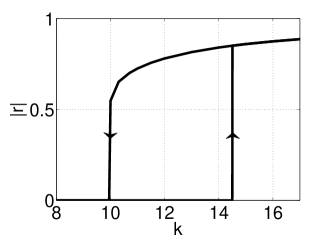
Figure 1: Hysteresis loop for $\omega_{0}=5,T=1$. The upper and lower branches correspond to stable coherent and incoherent states.

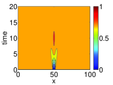
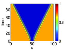
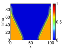
Figure 2: $|r(x,t)|$ for, (a) an initial configuration with a small part of the one-dimensional spatial domain in the incoherent state (blue) and a large part in the coherent state (orange), (b) a larger part of the spatial domain is initially in the incoherent state than that in (a), and (c) a still larger initial incoherent region. ($\omega_{0}=5,T=1,D=100,k=12$).

Next, we consider the dynamics as a function of the coupling strength $k$. Recall from Fig. 1 that there is a hysteretic region of coexisting coherent and incoherent states for the region $k^{\prime}_{c}<k<k_{c}$ where $k^{\prime}_{c}=10$ and $k_{c}=14.5$. Figure 3 shows the time evolution of $|r(x,t)|$ as a function of $k$. When the state is initialized with half ($25\leq x\leq 75$) the domain in the homogeneous incoherent state and the remaining half in the homogeneous coherent state, it is seen that if $k$ is sufficiently close to $k^{\prime}_{c}$, then the incoherent region engulfs the coherent region, while if $k$ is sufficiently greater than $k_{c}$, the homogeneous coherent solution takes over, and by comparing Figs. 3(a) to 3(e), we find that the propagation velocity decreases as $k$ is increased toward $k_{c}$. As $k$ increases past $k\sim 12$, the simple propagating front phenomenon seen in Figs. 2 and 3(a)-3(c) is replaced by more complex behavior. For example, in Fig. 3(d) we observe the formation of a “bridge” at $k=13$ ($<k_{c}$), i.e., a narrow stable coherent region sandwiched between two broad incoherent regions. This solution is apparently a long-time stable state. It develops as the two propagating fronts collapsing the coherent regions slow to a halt as they approach each other. We note further that the bridge has an amplitude which is smaller than that of the stable homogeneous solution, and the oscillation frequency is different as well (graphs not shown). Further, this bridge type solution persists for $k>k_{c}$, and can give rise to further intriguing dynamics like multiple bridges, as shown in Figs. 3(g), and even more vigorous behaviors of merging and re-creation of plateaus of coherent regions and bridges, as seen in Fig. 3(h). Comparing Fig. 3(f) to 3(h), it is notable that a wide variety of evolutionary behaviors occurs within a relatively small range in $k$, including the formation of single and multiple bridges, as well as collapse and re-creation of plateaus. Figure 4 studies the glassy-like behavior related to that seen in Fig. 3(h) at a slightly different set of system parameters. The figure shows plateaus of coherent regions (orange triangles in Figs. 4(a) and 4(b)) and bridge-like patterns (yellow stripes), connected through dynamical creation, merging and re-creation of such structures until the system eventually evolves into the homogeneous coherent state. Figure 4(c) shows the phase evolution inside the plateau region (orange triangle) of Fig. 4(a) centered at $t\approx 420,x\approx 50$. Figure 4(d) shows the phase evolution corresponding to the four-bridge-structure between the top of Fig. 4(a) and the bottom of Fig. 4(b) ($700\leq t\leq 1300$). We note that within a plateau, the whole region oscillates roughly homogeneously (see the nearly parallel evolving fronts in Fig. 4(c)), and each bridge pattern functions as a sink of incoming waves (see the zig-zag-like pattern in Fig. 4(d)). Further important dynamical characteristics during this vigorous glassy-like transition state are revealed in Figs. 4(e) and 4(f), which show $|r|$ and $\theta$ (where $r=|r|e^{i\theta}$) respectively at $t=148$. We see that there are multiple hole-like patterns (deep dips in $|r|$ in Fig. 4(e)), at which the phase changes sharply, (see Fig. 4(f), and note that the changes in phase for the outer two holes appear to be virtually discontinuous, as discussed in more detail shortly). In comparison, for the multiple-bridge region at $t=1200$, Figs. 4(g) and 4(h) show that both $|r|$ and $\theta$ change smoothly in space.

Figure 5 shows the dynamical characteristics associated with the hole-like patterns in another setting where these patterns dominate and are not interspersed with other spatial features (like bridges and plateaus). The figure corresponds to the same parameters as those in Fig. 3(h), but initialized with different incoherent and coherent regions. Compared with Fig. 3(h), there is a relatively short time for the system to stay in the plateau-like regions, and instead of settling in the homogeneous coherent state solution as in Fig. 3(h), four distinct hole-like patterns emerge (black lines starting at $t\approx 130$ in Fig. 5(a)). As time evolves, the two inner holes move toward each other and annihilate, while the outer two continue to evolve, apparently becoming stationary. Note also that for the two merging holes, they approach each other at a faster speed when they are closer to each other. Examination of the phase evolution of the system (Figs. 5(b) and 5(e)) suggests the center of each hole act as a source of plane waves, in contrast with the bridge solution which acts as a sink (see Fig. 4(d)). For the inner two moving holes, while each is characterized by a dip in magnitude (see Fig. 5(c) at $t=192$), the dips decrease in magnitude as the two holes approach each other, with the relative phase difference on the two sides of the hole center close to being continuous (see Fig.5(d)). However, if the holes are stationary, e.g., the outer two holes in Figs. 5(c) and 5(f), each dip in $|r|$ is close to zero, with the relative phase difference on the two sides being an essentially discontinuous slip of $\pm 3\pi$. A further observation in the case of two stationary holes is that there is a bump in $|r|$ half-way between them corresponding to the location at which incoming waves emitted from the holes converge (see $x=50$ in Fig. 5(f)).

In fact, when $k\approx k_{c}$, the hole-like pattern is a feature that shows up readily when two plane waves with a relative phase difference of $\pm\pi$ (or odd-multiples of them) collide. An example is studied in Fig. 6 where two waves of relative phase difference $\pi$ collide giving rise to a hole pattern. This observation is consistent with the relative phase differences observed at the two outer holes studied in Fig. 5(g). Furthermore, although the hole pattern seems to arise only under relatively specific conditions, it is found to be pretty stable with respect to changes in parameters or small perturbations once it is formed. Finally, as shown in Fig. 7, we note that the hole core occupies a finite width and so is not a point singularity when $T\neq 0$. This will be shown to have a close correspondence with the spiral wave in our two-dimensional study (sec. III.3).

It is further interesting to note some similarity between our observations in the region $k\approx k_{c}$ and the intermittency regime of the complex Ginzburg-Landau equation (CGLE) (See for example, section III of Ref. Aranson , and section 2.5 of Ref. Mori_Kura ). There, the CGLE displays similar glassy-like transition patterns characterized by large plateaus of coherent regions with hole-like patterns being continuously created and destroyed. However, there are also differences between the two systems. For example, the CGLE does not seem to have a close counterpart to the bridge pattern observed in our system, while more intricate dynamics of hole creation and destruction leading to zigzagging holes and defect chaos have not been observed in our study.

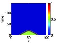
(a) $k=10$

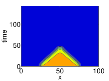
(b) $k=11$

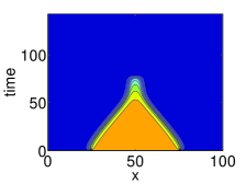
(c) $k=12$

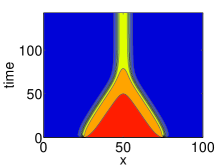
(d) $k=13$

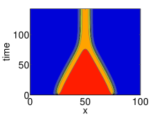
(e) $k=14$

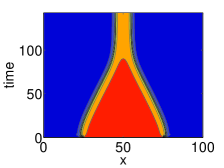
(f) $k=14.5$

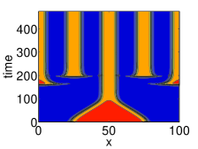
(g) $k=14.6$

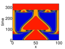
(h) $k=14.8$

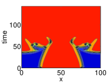
(i) $k=15$

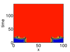
(j) $k=16$

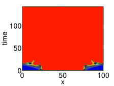
(k) $k=17$

Figure 3: A comparison of the time evolutions of $|r(x,t)|$ for different values of $k$ where $r$ is initialized with half of the interval at the coherent state ($25\leq x\leq 75$) and half at the incoherent state. Notice the difference in time scales of Fig. 3(g) and Fig. 3(h) from other figures ($\omega_{0}=5,T=1,D=100$; periodic boundary conditions are imposed).

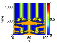
(a) $|r(x,t)|$

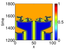
(b) $|r(x,t)|$

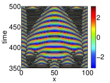
(c) $\theta(x,t)$ in the plateau centered at $x=50$ and $t=420$.

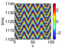
(d) $\theta(x,t)$ in part of the multiple-bridge pattern for $700\leq t\leq 1300$.

(e) $|r(x,148)|$

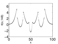
(f) $\theta(x,148)$

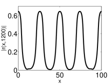
(g) $|r(x,1200)|$

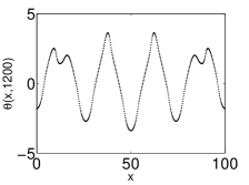
(h) $\theta(x,1200)$

Figure 4: (a,b) Glassy state of transition, formation of plateaus of coherent regions and hole patterns, and final evolution into the homogeneous coherent state. (c,d) Phase evolution in the plateau and multiple-bridge regions. (e,f) $|r(x,148)|$ and $\theta(x,148)$. (g,h) $|r(x,1200)|$ and $\theta(x,1200)$ ($\omega_{0}=4,T=1,D=100,k=10.3\hskip 2.84526pt(>k_{c}=10)$; initial condition: $r$ is given by the homogeneous coherent state solutions for $25\leq x\leq 75$, and $r=0$ otherwise; periodic boundary conditions are imposed).

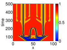
(a) $|r(x,t)|$

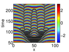
(b) $\theta(x,t)$

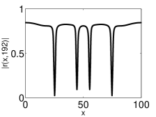
(c) $|r(x,192)|$

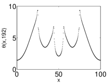
(d) $\theta(x,192)$

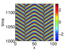
(e) $\theta(x,t)$

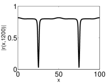
(f) $r(x,1200)$

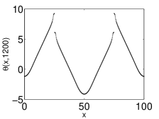
(g) $\theta(x,1200)$

Figure 5: Formation and dynamical evolution of hole patterns. (a) $|r(x,t)|$. (b-d) Close-up views of four hole patterns with two inner traveling holes. (e-g) Close-up views of two stationary hole patterns. ($\omega_{0}=5,T=1,D=100,k=14.8$; initial condition: $r$ is given by the homogeneous coherent state solutions for $0\leq x\leq 41$ and $59\leq x\leq 100$, and $r=0$ otherwise; periodic boundary conditions are imposed).

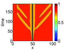
(a) $|r(x,t)|$

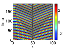
(b) $\theta(x,t)$

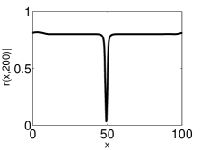
(c) $|r(x,200)|$

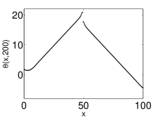
(d) $\theta(x,200)$

Figure 6: An example of the hole solution by collision of two plane wave solutions. The two waves meet at $x=50$ with a $\pi$ phase difference. ($\omega_{0}=5,T=1,D=100,k=14.8$ and periodic boundary conditions). The initial condition corresponds to a discontinuous $r$ given by a right traveling plane wave solution with $m=3$ (where the wave number is $2m\pi/D$) for $0\leq x\leq 50$ and a left traveling plane wave solution with $m=4$ for $50<x\leq 100$. Correspondingly, we observe from (d) that $[\theta(0,200)-\theta(100,200)]=2\pi$.

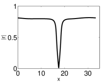
(a) $|r(x)|$

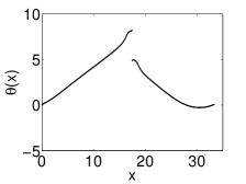
(b) $\theta(x)$

Figure 7: Finite width of (one-dimensional) hole core ($\omega_{0}=5,T=1,D=33.3,k=14.8$).

III.2 2D propagating fronts and “bridge” patterns

Figures 8 and 9 show the $d=2$ counterparts to the $d=1$ propagating fronts and associated features. Similar to what was previously done for $d=1$, half of the system is initialized in the homogeneous incoherent state and the remaining half in the homogeneous coherent state, and they are divided by a sinusoidally wiggling boundary (Figs. 8(a) and 9(a)). Analogous to the $d=1$ case, for $d=2$, the homogeneous incoherent state and homogeneous coherent state take over when $k$ is sufficiently small or large compared to $k_{c}$ respectively. The most interesting behaviors again take place when $k\approx k_{c}$. With $k=14.4<k_{c}$, Fig. 8 shows the development of a stable bridge solution. In contrast, with $k=14.8>k_{c}$, Fig. 9 shows a surprisingly rich spatio-temporal pattern evolution. As in Fig. 8, the originally coherent half apparently starts to shrink into a bridge (see Fig. 9(b)); however, as time progresses further, we see that coherent regions arise out of the originally incoherent regions to form new features (see also Figs. 3(g) and 3(h) in the $d=1$ case), and these new features interact in a nontrivial two dimensional manner. For example, when two neighboring coherent regions get close to each other, they can form bonds and merge into each other: see the connections formed between bridge-like structures from $t=83$ to $t=98$; also see the coherent spot formed at the upper left hand corner at $t=245$ and see how it merges into the bridge on its right as time progresses to $t=400$. We also observe that, during the process of merger, bridge-like structures may also temporarily separate and then re-connect: see the connecting bridge at the bottom right hand corner from $t=138$ to $t=170$. A further notable feature is the coherent spot on the top left hand corner at $t=561$ (a target pattern in the phase plot as shown in the next section), which survives from $t=561$ to the end of the numerical run. In the above reported numerical experiments we observe that both incoherent and coherent regions coexist for a long time. We do not know, however, whether a coherent or incoherent state ultimately will take over the whole domain at longer time.

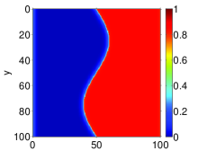
(a) $t=0$

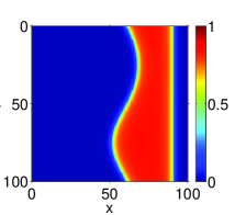
(b) $t=46$

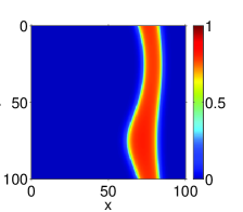
(c) $t=72$

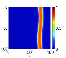
(d) $t=216$

Figure 8: Time evolution of $|r({\bf x},t)|$ of a $d=2$ configuration initialized with half of the region at the incoherent state and half at the coherent state divided by a wiggled boundary with $k=14.4$ ($<k_{c}=14.5$) ($\omega_{0}=5,T=1,D=100$; periodic boundary conditions are imposed).

(a) $t=0$

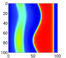
(b) $t=55$

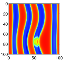
(c) $t=83$

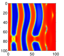
(d) $t=98$

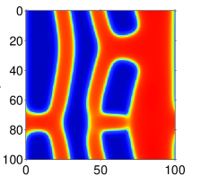
(e) $t=138$

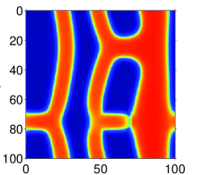
(f) $t=150$

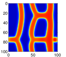
(g) $t=170$

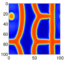
(h) $t=245$

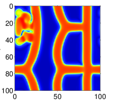
(i) $t=282$

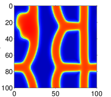
(j) $t=303$

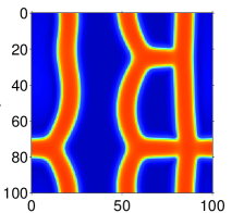
(k) $t=400$

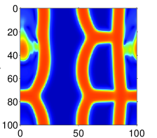
(l) $t=431$

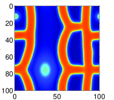
(m) $t=561$

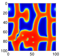
(n) $t=611$

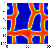
(o) $t=669$

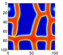
(p) $t=700$

Figure 9: Time evolution of $|r({\bf x},t)|$ from an initial configuration (a) with half of the region at the incoherent state and half at the coherent state divided by a wiggled boundary with $k=14.8$ ($>k_{c}=14.5$). A comparison with Fig. 8 shows a much richer spatio-temporal dynamical pattern ($\omega_{0}=5,T=1,D=100$; periodic boundary conditions are imposed).

III.3 2D Spots, spiral waves and target patterns

Figure 10 shows the time evolution of both $|r({\bf x},t)|$ and $\sin[\theta({\bf x},t)]$ $[$ where $r({\bf x},t)=|r({\bf x},t)|\exp[i\theta({\bf x},t)]$, and ${\bf x}=(x,y)$ in $2D$ $]$ when the system is initialized with a small random initial condition at each grid point, and the coupling strength is $k=15.5$ ($>k_{c}=14.5$). As expected from our previous studies, when $k>k_{c}$, coherent regions ($|r|\approx 1$) emerge from the initial incoherent state. Further, the phase plots show some distinct target-like patterns of nested closed surfaces of constant phase (see $t=40$ and $t=217$). As time progresses, coherent regions (red in the $|r|$ plots) become dominant and only small islands of incoherent regions remain (blue in the $|r|$ plots). Similar to our previous observation of propagating fronts when $k>k_{c}$ (compare Figs. 9(g) and 9(h)), coherent regions can form in an originally incoherent region ($|r|\ll 1$). For example, see the figures from $t=139$ to $t=161$, and especially from $t=195$ to $t=225$, where we see coherent regions (red/yellow) appearing and growing in the interior of incoherent (blue) blob, eventually destroying it. As can be inferred by comparing the $|r|$ and $\sin(\theta)$ plots, small blue, dot-like features in the $|r|$ plots represent phase defects in the complex amplitude (i.e., counter clockwise encirclement of such a feature leads to a phase change of either $+2\pi$ or $-2\pi$), and these blue dot features are commonly seen as spiral wave type patterns in the phase plots. When, as in the previously noted plots from $t=195$ to $225$, coherent regions take over from an incoherent patch, we also note that a number of phase defects result (which must be formed in opposite-spiral-parity pairs due to the conservation of topological charge); see $t=250$. The isolated phase defects subsequently wander about, and some of them are seen to annihilate with others of opposite parity (see the two defects closest to the bottom of the picture at $t=267$ and their evolution up to $t=293$), or sometimes they are absorbed into an incoherent region (e.g., compare the $|r|$ plots at $t=195$ and $t=217$). Lastly, regarding the speed of motion of spiral patterns, we note that similar to the observation in Fig. 5(a), when oppositely charged spirals get close enough to each other, their speed of approach becomes distinctively faster till they annihilate each other.

In studies of the CGLE, the hole pattern and spiral wave pattern are analogous phenomena occurring in $d=1$ and $d=2$, respectively. Indeed, the hole pattern and spiral wave pattern exhibit similar characteristics in our study. Both features are stable with respect to small changes in parameters, and exhibit similar dynamical characteristics of approach and annihilation as described above. In addition, Fig. 11 shows, in parallel with Fig. 7, that the central core of the spiral wave pattern occupies a finite area when $T\neq 0$. This is similar to the chimera-centered spirals noted in Refs. Martens ; KSB .

III.4 2D pulsating pattern

Another class of local coherent structures supported in the $d=2$ case is shown in Figs. 12 and 13, which shows a localized pulsating spot in an incoherent background. It is interesting to notice that oscillations of the magnitude and phase (which show up in the form of target patterns) of $r(x,t)$ are not the same, with that of the phase oscillation being more irregular and more than an order of magnitude faster than the amplitude oscillation (Figs. 12(d) and 13(g)). It is interesting to note that for the CGLE, stable pulsating patterns come only with the addition of a quintic term (see Ref. Deissler , and the later work Ref. Akh and references therein).

IV Summary and Concluding Remarks

In this paper, we have studied the spatio-temporal dynamics of spatially coupled oscillator systems where the oscillators have a heterogeneous distribution of response times. Using the results of Refs. OA1 -OA3 , we have derived a macroscopic PDE description for this situation [Eqs. (30)-(32)]. The resulting macroscopic dynamics are found to exhibit a wide variety of pattern formation behaviors. We characterized the possible behaviors roughly according to the hysteresis loop corresponding to bistable homogeneous incoherent and homogeneous coherent state solutions. Numerical studies show that the system behaviors for $k$ sufficiently below/above the bistable $k$-range are simple in that the homogeneous incoherent/coherent state eventually takes over the entire domain. In contrast, for $k$ in or near the bistable range the system can exhibit a variety of interesting spatio-temporal phenomena. These include propagating fronts, bridge patterns, hole patterns ($d=1$), spiral waves ($d=2$), spots, target patterns, pulsating patterns, etc.

Finally, it is interesting to consider the role of time delay in contributing to the features that we observed. If there is no time delay (i.e., $T=0$), there is no homogeneous bistable behavior as observed in Fig. 1, and the transition from the homogeneous incoherent state to the homogeneous coherent state is supercritical and takes place at $k_{c}=2\Delta$. In this case, many of the interesting spatio-temporal phenomena that we have found for $T>0$ are absent. For example, when $T=0$, the intricate 1D glassy state transitions were not observed, and the system typically evolves relatively rapidly into either homogeneous incoherent or homogeneous coherent state solutions. The 2D waves arisen from topological defects are still present; however, for $T=0$ the system will be similar to the case of zero nonlinear dispersion in Ref. Shima_Kura , where the incoherent core remains a point defect but not a finite area as observed when $T\neq 0$. Thus finite response time introduces additional dynamics, leading to the large variety of behaviors observed.

Acknowledgments. Work at the University of Maryland was supported by a MURI grant (ONR N00014-07-1-0734). Work at the University of Colorado was supported by the NSF (DMS 1030586).

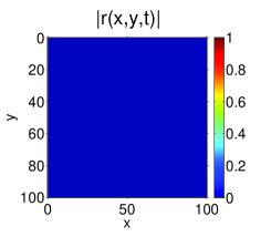
(a) $t=0$

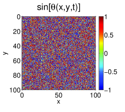
(b) $t=0$

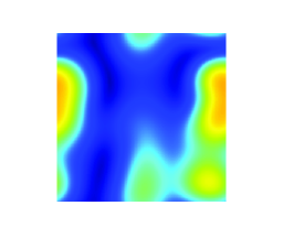
(c) $t=40$

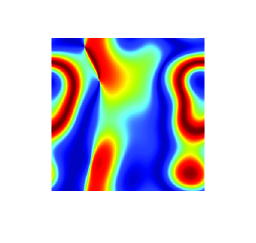
(d) $t=40$

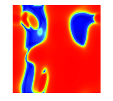
(e) $t=57$

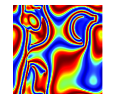
(f) $t=57$

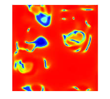
(g) $t=87$

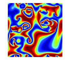
(h) $t=87$

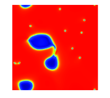
(i) $t=139$

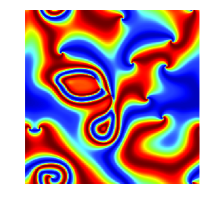
(j) $t=139$

Time evolution of $|r({\bf x},t)|$ and $\sin[\theta({\bf x},t)]$ (where $r({\bf x},t)=|r({\bf x},t)|\exp[i\theta({\bf x},t)]$) from random initial condition, (a) and (b) ($\omega_{0}=5,T=1,D=100,k=15.5\hskip 2.84526pt(>k_{c}=14.5)$; periodic boundary conditions are imposed).

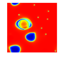
(k) $t=153$

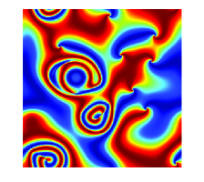
(l) $t=153$

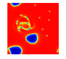
(m) $t=161$

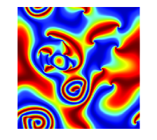
(n) $t=161$

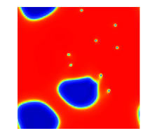
(o) $t=195$

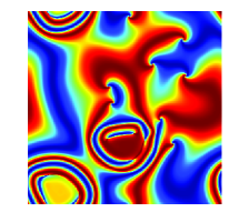
(p) $t=195$

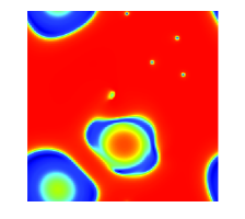
(q) $t=217$

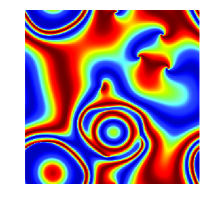
(r) $t=217$

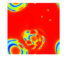
(s) $t=225$

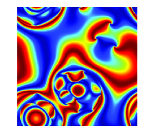
(t) $t=225$

*Cont’d

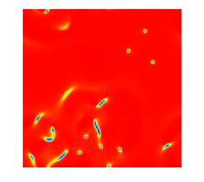
(u) $t=238$

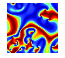
(v) $t=238$

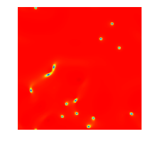
(w) $t=250$

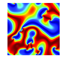
(x) $t=250$

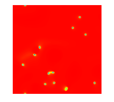
(y) $t=259$

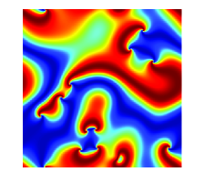
(z) $t=259$

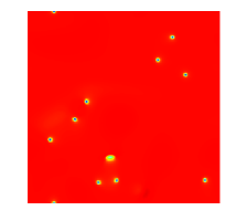
(aa) $t=263$

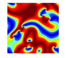
(ab) $t=263$

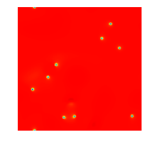
(ac) $t=267$

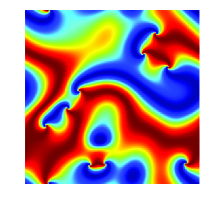
(ad) $t=267$

*Cont’d

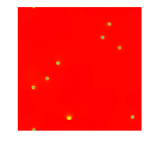
(ae) $t=281$

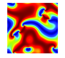
(af) $t=281$

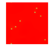
(ag) $t=293$

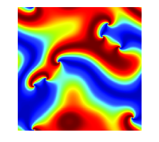
(ah) $t=293$

Figure 10: Cont’d

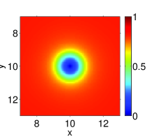
(a) $|r({\bf x})|$

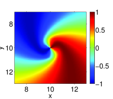
(b) $\sin(\theta({\bf x}))$

Figure 11: Finite area of (two-dimensional) spiral cores ($\omega_{0}=5,T=1,D=20,k=15$).

(a) $|r({\bf x},129)|$

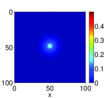
(b) $|r({\bf x},148)|$

(c) $|r({\bf x},158)|$

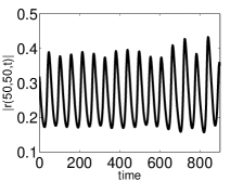
(d) $|r(50,50,t)|$

Figure 12: Pulsating pattern: amplitude variation. Figures (a) to (c) show approximately one “period” of oscillation in $|r|$. Figure (d) shows the time variation of $|r|$ at the center of the pulse; compare with Fig. 13 for oscillations in phase ($\omega_{0}=5,T=1,D=100,k=14.52$; periodic boundary conditions are imposed).

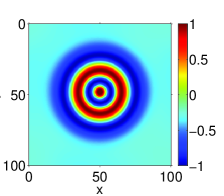
(a) $\sin(\theta),t=129$

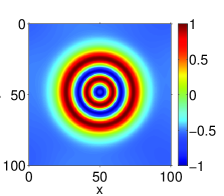
(b) $\sin(\theta),t=130$

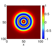
(c) $\sin(\theta),t=131$

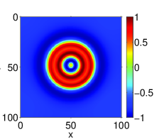
(d) $\sin(\theta),t=132$

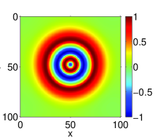
(e) $\sin(\theta),t=133$

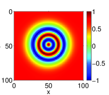
(f) $\sin(\theta),t=134$

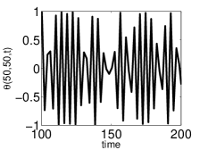
(g) $\sin(\theta(50,50,t))$

Figure 13: Pulsating pattern: phase variation. Figures (a) to (f) show the rapid time variations of the phase. Figure (g) shows the time variation of $sin(\theta)$ at the center of the pulse (Parameters are as indicated in Fig. 12).

References

- (1) A. Pikovsky, M. Rosenblum and J.Kurths, Synchronization: A Universal Concept in Nonlinear Sciences (Cambridge University Press, 2004).
- (2) S. Strogatz, Sync: The Emerging Science of Spontaneous Order (Hyperion 2003).
- (3) A. T. Winfree, The Geometry of Biological Time, ed. (Springer 2001).
- (4) J. Buck, Q. Rev. Biol. 63, 265 (1988).
- (5) S. H. Strogatz, D. M. Abrams, A. McRobie, B. Eckhardt and E.Ott, Nature 438, 43 (2005).
- (6) L. Glass and M. C. Mackey, From Clocks to Chaos: The Rhythms of Life (Princeton University Press, NJ, 1988).
- (7) T. D. Frank, A. Daffertshofer, C. E. Peper, P. J. Beek and H. Haken, Physica D 144, 62 (2000).
- (8) J. Garcia-Ojalvo, M. B. Elowitz and S. H. Strogatz, Proc. Natl. Acad. Sci. 101, 10955 (2004).
- (9) S. Yamaguchi, et al., Sci. 302, 255 (Oct. 10, 2003).
- (10) Y. Kuramoto, Chemical Oscillations, Waves, and Turbulence (Dover Press, Springer, 1984).
- (11) I. Z.Kiss, Y. Zhai and J. L. Hudson, Sci. 296, 1676 (2002).
- (12) A. F. Taylor, M. R. Tinsley, F. Wang, Z. Huang and K. Showalter, Sci. 323, 614 (2009).
- (13) H. Hong, M. Y. Choi and B. J. Kim, Phys. Rev. E 65, 026139 (2002).
- (14) T. Ichinomiya, Phys. Rev. E 70, 026116 (2004).
- (15) Y. Moreno and A. F. Pacheco, Europhys. Lett. 68, 603 (2004).
- (16) J. G. Restrepo, E. Ott and B. R. Hunt, Chaos 16, 015107 (2005).
- (17) Y. Kuramoto and D. Battogtokh, Nonlinear Phenom. Complex Syst. 5, 380 (2002).
- (18) S. Shima and Y. Kuramoto, Phys. Rev. E 69, 036213 (2004).
- (19) D. A. Abrams and S. H. Strogatz, Int. J. Bifur. Chaos 16, 21 (2006).
- (20) C. R. Laing, Physica D 238, 1569 (2009).
- (21) M. K. S. Yeung and S. H. Strogatz, Phys. Rev. Lett. 82, 648 (1999).
- (22) M. Y. Choi, H. J. Kim, D. Kim and H. Hong, Phys. Rev. E 61, 371 (2000).
- (23) W. S. Lee, E. Ott and T. M. Antonsen, Phys. Rev. Lett. 103, 044101 (2009).
- (24) E. Ott and T. M. Antonsen, Chaos 18, 037113 (2008).
- (25) E. Ott and T. M. Antonsen, Chaos 19, 023117 (2009).
- (26) E. Ott, B. Hunt, and T.M. Antonsen, arXiv:1005.3319.
- (27) G. C. Sethia and A. Sen, Phys. Rev. Lett. 100, 144102 (2008).
- (28) S. Chapman and T. G. Cowling, The Mathematical Theory of Non-uniform Gases (Cambridge University Press, 1952).
- (29) I. S. Aranson and L. Kramer, Rev. Mod. Phys. 74, 99 (2002).
- (30) H. Mori and Y. Kuramoto, Dissipative Structures and Chaos (Springer 1998).
- (31) E. A. Martens, C. R. Laing and S. H. Strogatz, Phys. Rev. Lett 104, 044101 (2010).
- (32) Y. Kuramoto, S. Shima, D. Battogtokh and Y. Shiogai, Prog. Theor. Phys. Suppl. 161, 127 (2006).
- (33) R. J. Deissler and H. R. Brand, Phy. Rev. Lett. 72, 478 (1994).
- (34) N. Akhmediev, J. M. Soto-Crespo and G. Town, Phy. Rev. E 63, 056602 (2001).