Solve the Master Equation by Python-An Introduction to the Python Computing Environment

Abstract

A brief introduction to the Python computing environment is given. By solving the master equation encountered in quantum transport, we give an example of how to solve the ODE problems in Python. The ODE solvers used are the ZVODE routine in Scipy and the bsimp solver in GSL. For the former, the equation can be in its complex-valued form, while for the latter, it has to be rewritten to a real-valued form. The focus is on the detailed workflow of the implementation process, rather than on the syntax of the python language, with the hope to help readers simulate their own models in Python.

I Introduction

Python is a general purpose, high-level programming language. It is well documented and easy to learn. With its concise and high-readable code, it greatly improves the efficiency of code development and code reuse, so we can save our time by simulating our model in Python.

In computation, Python provides us with an easy-to-use environment which saves both the code development time and the code execution time. Though it is an interpreted language, which means its execution speed is lower compared with the compiled language like C and Fortran, its performance has been greatly improved by a set of specific packages designed for numerical computation. This is done by gluing well behaved numerical libraries written in C/C++ and Fortran and allowing users to use them in Python code, thus we can write code efficiently in Python and get an execution speed like C and Fortran. Those packages includes Numpy Jones et al. (01); Oliphant (2007), Scipy Jones et al. (01); Oliphant (2007), Pygsl pyg , Cython Behnel et al. (2011) and various others packages. Numpy is based on the compiled LAPACK libraries that is standard for linear algebra computations. It provides the data structure ’array’ and fast operations on arrays, such as linear algebra, Fourier transform and random number generation, which make it easier and faster to handle matrix related problems. As the computation is essentially executed in LAPACK, it can run almost as fast as in the C code. Based on Numpy, Scipy provides many modules to perform the common tasks in science and industry, such as FFT, sparse matrix, statistics, signal processing and ODE solvers. The functionality of Numpy and Scipy is similar to Matlab, but they are developed to make scientific computing a natural part of Python, rather than be a copy of Matlab. Pygsl is a python interface to the GNU Scientific Library (GSL) Galassi et al. (2003), which is an open source C library for numerical computations in science. The models can be expresed in Numpy arrays and then by Pygsl we can use the functions in GSL directly as if they are Python functions, which greatly simplifies the usage of GSL functions. Cython is based on Python, but it allows for static C type declarations and direct calling of C or C++ functions, which combines the high productivity of Python with the execution speed of C Behnel et al. (2009). Cython is used in the development of the powerful computing software sage Stein et al. (2011) (or sagemath). Besides computation, there are many powerful visualization tools in Python, such as Visual vpy for animation and Matplotlib Hunter (2007) for Matlab-like plot. Other plotting tools, such as Mayavi may for 3D visulization and gnuplot Thomas et al. for scientific plot, can also be used in Python directly.

Even though there is very few cases where no package exists for performance improvement, we still recommend Python as it could save lots of our time in code development, while using the compiled languages can take lots of human time and would be exhausting. On the other hand, Python allows us to write the time consuming part of the algorithm, usually long loops, directly in compiled languages like C/C++ and Fortran, so we can get an optimal balance between human time and machine time. This can be done by lots of powerful wrappers, such as F2PY Peterson (2009), which can automatically wrap Fortran codes and make it callable from Python, and Weave Wea , which makes it possible to written C and C++ codes directly in Python codes.

In this paper, we will use Python to solve the master equation in reference Greentree et al. (2004), which is an ordinary differential equation (ODE). This is an introduction to the Python computing environment and a detailed example of solving the ODE problems in Python. We will use three solvers, the ZVODE routine in Scipy, the bsimp solver and the rkf45 solver of GSL to solve it. We will also give an example of using Cython to optimize the code to get faster execution speed. The emphasis is layed on the workflow of how to solve the ODE problems in Python rather than on the syntax of this language. One can turn to the books Fangohr et al. (2008); Landau (2008); Kiusalaas (2010) for a detailed tutorial of computational physics in Python.

II The Master Equation

The master equation to be solved is

$$\dot{\rho}=-i\left[\mathcal{H},\rho\right]-\Gamma\left[\rho-diag(\rho)\right],$$ (1)

where the Hamiltonian $\mathcal{H}=\left(\begin{array}[]{ccc}0&-\Omega_{12}&0\\ -\Omega_{12}&0&-\Omega_{23}\\ 0&-\Omega_{23}&0\end{array}\right)$ describes the coherent tunneling via adiabatic passage (CTAP) scheme, $\Gamma$ is the $T_{2}$ dephasing rate and $\Omega_{12}$ and $\Omega_{23}$ are the tunneling rate between the corresponding quantum dots

$$\Omega_{12}\left(t\right) = \Omega^{max}\exp\left[-\left(t-\frac{t_{max}+\sigma}{2}\right)^{2}/\left(2\sigma^{2}\right)\right]$$

$$\Omega_{23}\left(t\right) = \Omega^{max}\exp\left[-\left(t-\frac{t_{max}-\sigma}{2}\right)^{2}/\left(2\sigma^{2}\right)\right].$$

This is an evolution equation of the density matrix of the system, which describes the evolution of the electron in the dots. The master equation is often used when the decoherence effect are considered due to the interaction between the system and its environment. The diagonal terms of the density matrix describe the population of the electron in the corresponding dots, while the off-diagonal terms describe the correlation between corresponding dots. For the $T_{2}$ dephasing term, the off-diagonal terms describe the decoherence of the electron, which corresponds to the loose of its quantum nature. The neglected diagonal terms in the dephasing terms describe the loss of particles in corresponding dots due to the interaction with the environment, which is not important in the CTAP scheme.

To judge the efficiency of the transporting system, this equation needs to be solved. We would first solve the case without the dephasing term using the solver ZVODE and bsimp, and only consider the case of counter-intuitive pulses, that is, the result shown in Figure.3(b) in reference Greentree et al. (2004). After that, we would solve the case with the dephasing term included using the rkf45 solver and give the pseudo-color plot correspoding Figure.4 in reference Greentree et al. (2004). The parameters are chosen as the same as there with $\sigma=t_{max}/8$. Reducing $t$ by $\pi/\Omega^{max}$, that is, $t=t/\left(\pi/\Omega^{max}\right)$ and $t_{m}=t_{max}/\left(\pi/\Omega^{max}\right)$, and then rescale $t$ to 1 by $t=t/t_{m}$, the equation is reduced to the form

$$\dot{\rho}=-i\pi t_{m}[\mathcal{H},\rho]-\Gamma\pi t_{m}[\rho-diag(\rho)],$$ (2)

where $\Gamma=\Gamma/\Omega^{max}$ and the coupling pulses are reduced to

$$\Omega_{12}\left(t\right) = \exp\left[-32\left(t-\frac{9}{16}\right)^{2}\right]$$

$$\Omega_{23}\left(t\right) = \exp\left[-32\left(t-\frac{7}{16}\right)^{2}\right].$$ (3)

This is the equation we need to solve in Python.

III The Solvers

Scipy provides two ODE solvers ’odeint’ and ’ode’ in its ’integrate’ module, with the former using the ’lsoda’ of the Fortran library odepack and the latter using the VODE ( for real-valued equations) and the ZVODE (for complex-valued equations) routines. The ZVODE routine provides the implicit Adams method for non-stiff problems and a method based on the backward odifferentiation formulas (BDF) for stiff problems. Stiff equation is that includes some terms that can lead to rapid vibration in the solution and it requires the step size to be taken extremely small if using non-stiff solvers. This would happen when the variables are changing on two vastly different scales. If you do not know whether you problem is stiff or not, using the stiff solvers would be safe, although it would cost more time. Here we will use the ZVODE routine with the BDF method. The CTAP scheme is non-stiff, but we use stiff solvers here just to give examples of how to use them. In the last part when we solve the equation with the dephasing effect, we would use the non-stiff solver and optimize it by Cython, as there is a hard requirement on computation time there. As the solver only accepts a set of equations that are in a vector form, we have to rewrite equation (2) from the matrix form to a one-dimensional array form. This can be done via the Numpy array and related operations. The equation finally should be in the form

$$\frac{dy}{dt}=-i\pi t_{m}f,$$ (4)

where $y$ is the column version of $\rho$ and $f$ is the derivative of $y$ with time.

Listing 1 impliments the solution of equation (4). We first import it by ’from Scipy.integrate import ode’, which imports the solver ode from Scipy’s integrate module. Then we define equation (4) and its Jacobian using the data structure array provided by Numpy, which is straightforward in describing matrix related problems . The integrator of the solver should be set to use the ZVODE routine with the BDF method. After setting the step size and the precision anticipated, we can call this solver to forward the calculation step by step until it reaches the final value. We can plot the data directly in Python using Matplotlib or gnuplot Haggerty . Here we output the data to a file and plot it in gnuplot. The source file of gnuplot would also be given in listing 2 and the result is shown in Figure. 1.

Listing 1: This program solves the CTAP regime without the dephasing term using the zvode routine of Scipy.

⬇

1#! /usr/bin/env python2.7

#First import the modulus used in this program. Numpy is so often used that perhaps every

3#program should import it first. The ode solver is in Scipy’s integrate modulus.

5import numpy

from scipy.integrate import ode

7

#Define function dy/dt = f. We have to write the elements of f out by hand, as

9#this solver requires the Jacobian, whose elements must be calculated by hand.

#For the rkf45 solver used below, which does not require the Jacobian, we can express it by

11#Numpy array operations without calculating its elements by hand.

def userSupply(t, y, tm):

13 j1=numpy.exp(-32.*(t-9./16)**2)

j2=numpy.exp(-32.*(t-7./16)**2)

15 #complex number is represented by j in Python. 5j means 5*i and 1j means i.

return -1j*numpy.pi*tm*numpy.array(

17 [j1*y[1]-j1*y[3], j1*y[0]+j2*y[2]-j1*y[4], j2*y[1]-j1*y[5],

j1*y[4]-j1*y[0]-j2*y[6], j1*y[3]+j2*y[5]-j1*y[1]-j2*y[7],

19 j2*y[4]-j1*y[2]-j2*y[8], j1*y[7]-j2*y[3],

j1*y[6]+j2*y[8]-j2*y[4], j2*y[7]-j2*y[5]])

21

#The jacobian df/dy of the ODE equations.

23def jac(t, y, tm):

j1=numpy.exp(-32.*(t-9./16)**2)

25 j2=numpy.exp(-32.*(t-7./16)**2)

return -1j*numpy.pi*tm*numpy.array([[0, j1, 0, -j1, 0, 0, 0, 0, 0],

27 [j1, 0, j2, 0, -j1, 0, 0, 0, 0],

[0, j2, 0, 0, 0, -j1, 0, 0, 0],

29 [-j1, 0, 0, 0, j1, 0, -j2, 0, 0],

[0, -j1, 0, j1, 0, j2, 0, -j2, 0],

31 [0, 0, -j1, 0, j2, 0, 0, 0, -j2],

[0, 0, 0, -j2, 0, 0, 0, j1, 0],

33 [0, 0, 0, 0, -j2, 0, j1, 0, j2],

[0, 0, 0, 0, 0, -j2, 0, j2, 0]])

35#initial time and value.

t0 = 0

37y0 = numpy.array([1, 0, 0, 0, 0, 0, 0, 0, 0], dtype=numpy.complex128)

#t_max and the step size.

39tm = 8000

H = 1.e-3

41#Call the solver ode with the function ’userSupply’ and the Jacobian ’jac’, and

#define the integrator ’zvode’ with the ’bdf’ method and set tolerance ’rtol’.

43r = ode(userSupply, jac).set_integrator(

’zvode’, method=’bdf’, with_jacobian=True, rtol=1.e-6, order=5)

45#Prepare the intial values and the parameters t_max.

r.set_initial_value(y0, t0).set_f_params(tm).set_jac_params(tm)

47

#define the file to write data to.

49output1=open(’dataCounBdf’,’w’)

#Forward the integrator in a loop and output the data to the file.

51while r.successful() and r.t < 1.:

if ( 1. - r.t) < H: H = 1. -r.t

53 r.integrate(r.t + H)

output1.write(”%f %f %f %f\n” % (r.t, r.y[0], r.y[4], r.y[8]))

55

output1.close() #close the file.

Listing 2: The program plots the evolution result.

⬇

1set terminal tikz standalone color size 5in,3in

set out ’counterBdf.tex’

3set xlabel ’$\frac{t}{tm}$’

set ylabel ’$\rho$’

5set yrange [-0.1:1.2]

set grid

7set title ’solution of the ZVODE routine’

plot ’dataCounBdf’ using ($1):($2) smooth csplines title ’$\rho_{11}$’, ’dataCounBdf’ using ($1):($3) smooth csplines title ’$\rho_{22}$’, ’dataCounBdf’ using ($1):($4) smooth csplines title ’$\rho_{33}$’

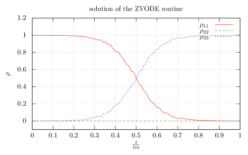
Figure 1: Solution got via the ZVODE routine for the counter-intuitive pulse without dephasing. The particle evolves from the first dot to the third dot without any population on the second dot. This is the result of the CTAP scheme, as explained in reference Greentree et al. (2004). Here $t_{m}$ has been set to 8000 to avoid vibrations of the lines.

GSL provides many ODE solvers, using the implicit Bulirsch-Stoer method, the Gear method and various Runge-Kutta methods. They can be used in Python via the Pygsl module, which makes their usage straightforward, just like using the solvers in Scipy, and you can read its document by typing ’help(’pygsl.odeiv’)’ in Python. Here the solver bsimp is used, which is given in listing 3. The bsimp solver impliments the implicit Bulirsch-Stoer method of Bader and Deuflhard. For smooth functions, the Bulirsch-Stoer method is the best way to achieve both high-accuracy solutions and computational efficiency Press (1994), with the implicit Bulirsch-Stoer method designed for stiff problems. As above, the Pygsl module should to be imported first. Then is the definition of the equation and its Jacobian. It should be noticed that the solvers in GSL only accept real-valued equations, so $y$’s real and imaginary part in equation (4) have to be separated and form a new set of coupled equations with 18 elements, with $y[2i]$ and $y[2i+1]$ the real and the imaginary part of the original$y[i]$. Their preparation is a little different from solvers in Scipy, which can be learned from its documentation. It only needs inputs of the initial step size and the errors tolerated, as the following step sizes are adjusted automatically to optimize its speed and precision. The gnuplot source code is as the code 2 except with a different input data name and output file name, so we do not put it here. The result is given in Figure. 2.

Listing 3: This program solves the CTAP regime without the dephasing using the bsimp solver of GSL.

⬇

1#! /usr/bin/env python2.7

#First import the modulus used in this program.

3#The solver is in pygsl’s odeiv module.

import numpy

5from pygsl import odeiv

7#User supplied function dy/dt = f. This is more complex compared with the above code.

#As we have to seperate the real and imaginary parts from the original equations.

9def userSupply(t, y, tm):

j2 = numpy.exp(-32.*(t-9./16)**2)

11 j1 = numpy.exp(-32.*(t-7./16)**2)

return numpy.pi*tm*numpy.array(

13 [j1*(y[3]-y[7]), j1*(y[6]-y[2]), j1*(y[1]-y[9])+j2*y[5],

j1*(y[8]-y[0])-j2*y[4], j2*y[3]-j1*y[11], j1*y[10]-j2*y[2],

15 j1*(y[9]-y[1])-j2*y[13], j1*(y[0]-y[8])+j2*y[12],

j1*(y[7]-y[3])+j2*(y[11]-y[15]), j1*(y[2]-y[6])+j2*(y[14]-y[10]),

17 j2*(y[9]-y[17])-j1*y[5], j2*(y[16]-y[8])+j1*y[4],

j1*y[15]-j2*y[7], j2*y[6]-j1*y[14], j1*y[13]+j2*(y[17]-y[9]),

19 -j1*y[12]+j2*(y[8]-y[16]), j2*(y[15]-y[11]), j2*(y[10]-y[14])])

21#the Jacobian df/dy and df/dt. The bsimp solver requires both df/dy and df/dt.

def jac(t, y, tm):

23 j2 = numpy.exp(-32.*(t-9./16)**2)

j1 = numpy.exp(-32.*(t-7./16)**2)

25 dj2dt = -64*(t-9./16)*j2

dj1dt = -64*(t-7./16)*j1

27 dfdy = numpy.zeros([18,18])

dfdy[0, 3] = j1; dfdy[0, 7] = -j1;

29 dfdy[1, 2] = -j1; dfdy[1, 6] = j1;

dfdy[2, 1] = j1; dfdy[2, 5] = j2; dfdy[2, 9] = -j1

31 dfdy[3, 0] = -j1; dfdy[3, 4] = -j2; dfdy[3, 8] = j1

dfdy[4, 3] = j2; dfdy[4, 11] = -j1

33 dfdy[5, 2] = -j2; dfdy[5,10] = j1

dfdy[6, 1] = -j1; dfdy[6, 9] = j1; dfdy[6, 13] = -j2

35 dfdy[7, 0] = j1; dfdy[7, 8] = -j1; dfdy[7, 12] =j2

dfdy[8, 3] = -j1; dfdy[8, 7] = j1; dfdy[8, 11] = j2; dfdy[8, 15] = -j2

37 dfdy[9, 2] = j1; dfdy[9, 6] = -j1; dfdy[9, 10] = -j2; dfdy[9, 14] = j2

dfdy[10, 5] = -j1; dfdy[10, 9] = j2; dfdy[10, 17] = -j2

39 dfdy[11, 4] = j1; dfdy[11, 8] = -j2; dfdy[11, 16] = j2

dfdy[12, 7] = -j2; dfdy[12, 15] = j1

41 dfdy[13, 6] = j2; dfdy[13, 14] = -j1

dfdy[14, 9] = -j2; dfdy[14, 13] = j1; dfdy[14, 17] = j2

43 dfdy[15, 8] = j2; dfdy[15, 12] = -j1; dfdy[15, 16] = -j2

dfdy[16, 11] = -j2; dfdy[16, 15] = j2

45 dfdy[17, 10] = j2; dfdy[17, 14] = -j2

dfdt = numpy.array(

47 [dj1dt*(y[3]-y[7]), dj1dt*(y[6]-y[2]), dj1dt*(y[1]-y[9])+dj2dt*y[5],

dj1dt*(y[8]-y[0])-dj2dt*y[4], dj2dt*y[3]-dj1dt*y[11], dj1dt*y[10]-dj2dt*y[2],

49 dj1dt*(y[9]-y[1])-dj2dt*y[13], dj1dt*(y[0]-y[8])+dj2dt*y[12],

dj1dt*(y[7]-y[3])+dj2dt*(y[11]-y[15]), dj1dt*(y[2]-y[6])+dj2dt*(y[14]-y[10]),

51 dj2dt*(y[9]-y[17])-dj1dt*y[5], dj2dt*(y[16]-y[8])+dj1dt*y[4],

dj1dt*y[15]-dj2dt*y[7], dj2dt*y[6]-dj1dt*y[14], dj1dt*y[13]+dj2dt*(y[17]-y[9]),

53 -dj1dt*y[12]+dj2dt*(y[8]-y[16]), dj2dt*(y[15]-y[11]), dj2dt*(y[10]-y[14])])

return numpy.pi*tm*dfdy, numpy.pi*tm* dfdt

55

#Initial values.

57dimension = 18

t = 0

59y = numpy.array([1, 0, 0, 0, 0, 0, 0, 0, 0, 0, 0, 0, 0, 0, 0, 0, 0, 0])

tm = 50

61

#the stepping function advances the solution from t_i to t_i+1 .

63#step_bsimp is the bsimp solver we use.

step = odeiv.step_bsimp(dimension,userSupply,jac,args=tm)

65#the control function optimizes the step size with the input tolerated errors.

control = odeiv.control_yp_new(step,1.e-6,1.e-6)

67#Based on the stepping and the control funtion, the evolve

#function advances the solution in a given interval.

69evolve = odeiv.evolve(step, control,dimension)

71#The file to store data.

output1=open(’dataInBsipmp’,’w’)

73

#initial step size. It can optimize step size under given errors. Only need to input an initial step size.

75h = 1.e-2

while t < 1.:

77 if (1. - t) < h: h=1. - t

t, h, y = evolve.apply(t, 1, h, y)

79 output1.write(”%f %f %f %f\n” % (t, numpy.sqrt(y[0]**2+y[1]**2), numpy.sqrt(y[8]**2+y[9]**2), numpy.sqrt(y[16]**2+y[17]**2)))

81#close file.

output1.close()

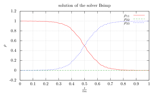
Figure 2: Solution got via the bsimp solver of GSL for the counter-intuitive pulse without dephasing. It’s the same as Figure. 1. $t_{m}$ also equals to 8000.

Now we add the dephasing term and solve the equation (2). This is done by the rkf45 solver of GSL, which uses the Runge-Kutta-Fehlberg method with adaptive stepsize control using the 5th order error estimate. The rkf45 method is the most general method and applies to almost all initial value ODE problems. The solution process gets greatly simplified using this solver, as it does not require the Jacobian of the system, the calculation of which takes most of our time. The Jacobian needs to do partial differentiation on the funtion $f$ of equation (4), which needs to be done by hand. Without it, we can use Numpy array operations to write the equation (2) to the one-dimensional array form (4) and do not need to calculate by hand at all, thus greatly saves our time. This can be done by substituting $\rho=\rho_{R}+i\rho_{C}$ into equation (2) and seperating the derivative of the $\rho_{R}$ and $\rho_{C}$. After rescaling, we would get the following equation

$$\frac{d\rho_{R}}{dt}=[H,\rho_{C}]-\Gamma[\rho_{R}-diag(\rho_{R})]$$

$$\frac{d\rho_{C}}{dt}=-[H,\rho_{R}]-\Gamma[\rho_{C}-diag(\rho_{C})].$$ (5)

This form can be expressed to the one-dimensional form easily in Numpy, as the listing 4 shows, which solves the equation with dephasing included.

To get the pseudo-color plot of Figure. 4 of reference Greentree et al. (2004). we need to solve the master equation (2) many times with different values of $\Gamma$ and $t_{m}$ each time. Here we solve it for $100x500$ times with $100$ different $\Gamma$ and $500$ different $t_{m}$. This is done in a loop and would cost huge computation time. We would give an Cython code to optimize the Python code, which is also an example of how to use Cython. The optimzed code with Cython is given in listing 6 in the next section. The gnuplot source code is given in listing 5 and the pseudo-color plot is shown in Figure. 3.

Listing 4: This program solves the CTAP regime with the dephasing included using the solver rkf45 of GSL.

⬇

1#! /usr/bin/env python2.7

#First import the modulus used in this program.

3#The solver rkf45 is in pygsl’s odeiv module.

import numpy

5from pygsl import odeiv

7#Abstract class used for declaration.

class Function:

9 def evaluate(self,t,y,lis):

tm,x=lis

11 return 0

#User supplied function dy/dt = f. We can use the Numpy array and related operations to define it, including array reshape and concatenate, which simplifys the process.

13class userSupply(Function):

def evaluate(self,t,y,lis):

15 tm,x=lis

j1 = numpy.exp(-32.*(t-9./16)**2)

17 j2 = numpy.exp(-32.*(t-7./16)**2)

H=numpy.array([[0,j1,0],[j1,0,j2],[0,j2,0]])

19 rhoR=y[0:9].reshape((3,3))

rhoC=y[9:18].reshape((3,3))

21 dRdt=numpy.dot(H,rhoC)-numpy.dot(rhoC,H)-x*(rhoR-numpy.diag(rhoR))

dCdt=numpy.dot(rhoR,H)-numpy.dot(H,rhoR)-x*(rhoC-numpy.diag(rhoC))

23 return numpy.pi*tm*numpy.concatenate((dRdt.reshape((9)),dCdt.reshape((9))))

25#compute_dephase impliments the loop within which the equation is solved with different parameters each time.

def compute_dephase(f,N1,N2):

27 output1=open(’dataDephase1’,’w’)

output2=open(’dataDephase2’,’w’)

29 output3=open(’dataDephase3’,’w’)

dimension=18

31 for x in numpy.linspace(0.,0.5,N1):

for tm in numpy.linspace(0,10,N2):

33 step = odeiv.step_rkf45(dimension,f.evaluate,args=(tm, x))

control = odeiv.control_yp_new(step,1e-7,1e-7)

35 evolve = odeiv.evolve(step, control,dimension)

y=numpy.zeros((dimension))

37 y[0]=1.0

t=0.;h = 1.e-4

39 while t<1.:

if (1.-t)<h: h=1.-t

41 t, h, y = evolve.apply(t,1.,h,y)

output1.write(” %f ” % y[0])

43 output2.write(” %f ” % y[4])

output3.write(” %f ” % y[8])

45 output1.write(”\n”)

output2.write(”\n”)

47 output3.write(”\n”)

output1.close()

49 output2.close()

output3.close()

51

compute_dephase(userSupply(),2,3)

Listing 5: The program plots the pseudo-color plot for the master equation with dephasing.

⬇

1set terminal post color enhanced

set out ’dephase1.ps’

3set xlabel ’t_{max}’

set ylabel ’{/Symbol G}’

5set xtics (”0” 0, ”2” 100,”4” 200,”6” 300,”8” 400, ”10” 500)

set ytics (”0” 0, ”0.1” 20,”0.2” 40,”0.3” 60,”0.4” 80, ”0.5” 100)

7set cbrange [0:1]

set pm3d map

9set title ’{/Symbol r}_{1}’

splot ’dataDephase1’ matrix

11exit

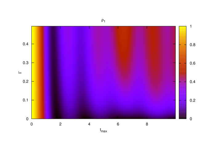
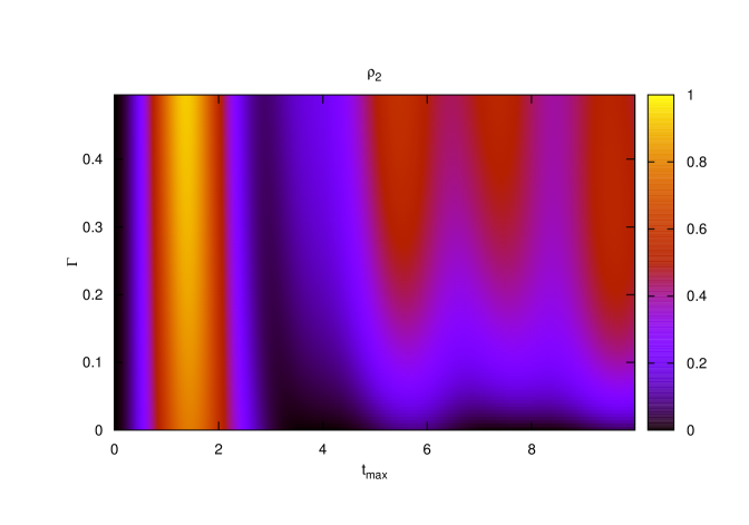
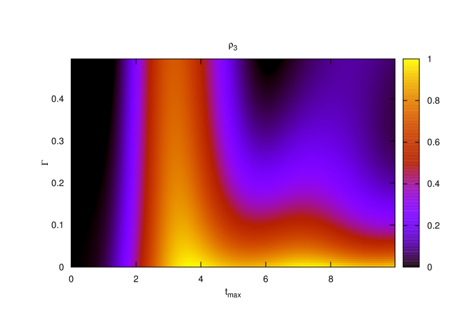
Figure 3: The pseudo-color plot of the master equation including the dephasing. See reference Greentree et al. (2004).

IV Cython

Cython allows C type declarations both for variables and functions, and you can use C functions from C libraries in Cython. It can improve the Numpy array operations, especially array iteration, to the speed of C array operations, so we can write code efficiently using Numpy array while get the speed of C. To use Cython, there are generally three stages. Firstly we typedefine the variables to C static types via the key word ’cdef’, which removes the dynamical nature of those variables and greatly improves the operation speed involving them. If their are Numpy arrays, we should also typedefine their type, which is shown in the listing 6. There are a static type and a dynamical type, both of which should be typedefined. After this first stage, the program would get a faster speed compared with the original one, especially when the iterator in the long loops are typedefined. The second stage is to typedefine the Python functions to return static type value via the key word ’cdef type-used function(tpye-used variable)’, where the type-used are appropriate types. This can greatly improve the speed of function calls, but now this function can only be called in Cython. If using the key word ’cpdef’, then the function can be called in Python. The function type defination can improve the behavior of the total code greatly. The last stage is to turn off some regular checks for some functions in the code, especially for inline functions. Well optimized Cython code can get an speed as fast as C and Fortran, as can be seen in the examples provided by the Cython website. For detailed documentation, turn to the reference  Behnel et al. (2011, 2009) and references there. The listing 6 below only serves as an example of how to use Cython. The list 7 shows the results of profiling the Python code and the Cython code. The cpu is ’2 Intel(R) Core(TM)2 Duo CPU T7500 @2.20GHz’. We can see that the Cython code saves about one third time compared with the Pythond code. The speed got is not very much compared with hundreds of times in examples provided by Cython documentation. There are two reasons for this. The first is that this is not optimizing a pure Python code. We have used many well behaved packages in the Python code, which is very fast already. The second is that our Cython code is not perfect. Many modifications can be done to optimize it further.

Listing 6: The Cythond code to optimize the Python one to get speed up.

⬇

1#! /usr/bin/env python2.7

#First import the modulus used in this program.

3#The solver rkf45 is in pygsl’s odeiv module.

5import numpy as np

cimport numpy as np

7from pygsl import odeiv

cimport cython

9

cdef extern from ”math.h”:

11 double exp(double)

@cython.profile(False)

13cdef inline double EXP(double x):

return exp(x)

15

DTYPE=np.float64

17ctypedef np.float64_t DTYPE_t

19#Abstract class used for declaration.

cdef class Function:

21 cpdef np.ndarray[DTYPE_t,ndim=1] evaluate(self,double t,np.ndarray[DTYPE_t,ndim=1] y, np.ndarray[DTYPE_t,ndim=1] lis):

cdef tm,x

23 tm,x=lis

cdef np.ndarray[DTYPE_t,ndim=1] a=np.zeros((18),dtype=DTYPE)

25 return a

27#User supplied function dy/dt = f. We can use the np array and related operations to define it, including array reshape and concatenate, which simplifys the process.

cdef class userSupply(Function):

29 cpdef np.ndarray[DTYPE_t,ndim=1] evaluate(self,double t,np.ndarray[DTYPE_t,ndim=1] y,np.ndarray[DTYPE_t,ndim=1] lis):

cdef tm,x

31 tm,x=lis

j1 = EXP(-32.*(t-9./16)**2)

33 j2 = EXP(-32.*(t-7./16)**2)

cdef np.ndarray[DTYPE_t,ndim=2] H=np.zeros((3,3),dtype=DTYPE)

35 H[0,1]=j1;H[1,0]=j1;H[1,2]=j2;H[2,1]=j2

rhoR=y[0:9].reshape((3,3))

37 rhoC=y[9:18].reshape((3,3))

dRdt=np.dot(H,rhoC)-np.dot(rhoC,H)-x*(rhoR-np.diag(rhoR))

39 dCdt=np.dot(rhoR,H)-np.dot(H,rhoR)-x*(rhoC-np.diag(rhoC))

return np.pi*tm*np.concatenate((dRdt.reshape((9)),dCdt.reshape((9))))

41

#compute_dephase impliments the loop within which the equation is solved with different parameters each time.

43cdef compute_dephase(Function f,double N1,double N2):

output1=open(’dataDephase1’,’w’)

45 output2=open(’dataDephase2’,’w’)

output3=open(’dataDephase3’,’w’)

47 cdef int dimension=18

cdef double x,tm

49 cdef double t,h

cdef np.ndarray[DTYPE_t,ndim=1] arg=np.zeros((2),dtype=DTYPE)

51 cdef np.ndarray[DTYPE_t,ndim=1] y=np.zeros((dimension),dtype=DTYPE)

for x in np.linspace(0.,0.5,N1):

53 for tm in np.linspace(0,10,N2):

arg[0]=tm;arg[1]=x

55 step = odeiv.step_rkf45(dimension,f.evaluate,args=arg)

control = odeiv.control_yp_new(step,1e-7,1e-7)

57 evolve = odeiv.evolve(step, control,dimension)

y[0]=1.0

59 t=0.;h = 1.e-4

while t<1.:

61 if (1.-t)<h: h=1.-t

t, h, y = evolve.apply(t,1.,h,y)

63 output1.write(” %f ” % y[0])

output2.write(” %f ” % y[4])

65 output3.write(” %f ” % y[8])

y=np.zeros((dimension),dtype=DTYPE)

67 output1.write(”\n”)

output2.write(”\n”)

69 output3.write(”\n”)

output1.close()

71 output2.close()

output3.close()

73

cpdef callFunction(Function f,double N1,double N2):

75 compute_dephase(f,N1,N2)

Listing 7: The result of profiling the Cython code and the Python one.

⬇

1#Profile result for dephaseCython.pyx.

#The CPU of my laptop is 2 Intel(R) Core(TM)2 Duo CPU T7500 @2.20GHz.

3Tue May 3 21:24:15 2011 Profile.prof

5 314988757 function calls in 4075.919 seconds

7 Ordered by: internal time

9 ncalls tottime percall cumtime percall filename:lineno(function)

3987941 2750.219 0.001 4032.149 0.001 {pygsl.__callback.gsl_odeiv_evolve_apply}

11 61192534 693.108 0.000 1281.930 0.000 twodim_base.py:220(diag)

61192534 229.666 0.000 413.172 0.000 numeric.py:216(asarray)

13 61192534 183.506 0.000 183.506 0.000 {numpy.core.multiarray.array}

122385068 175.650 0.000 175.650 0.000 {len}

15 1 23.031 23.031 4075.919 4075.919 {dephaseCython.callFunction}

3987941 17.043 0.000 4049.192 0.001 odeiv.py:421(apply)

17 50000 0.860 0.000 1.364 0.000 odeiv.py:385(__init__)

50000 0.392 0.000 0.649 0.000 odeiv.py:88(__init__)

19 200000 0.318 0.000 0.318 0.000 {hasattr}

50000 0.287 0.000 0.476 0.000 odeiv.py:407(__del__)

21 50000 0.273 0.000 0.439 0.000 odeiv.py:260(__del__)

50000 0.263 0.000 0.447 0.000 odeiv.py:110(__del__)

23 50000 0.195 0.000 0.317 0.000 odeiv.py:365(__init__)

50000 0.166 0.000 0.166 0.000 {pygsl.__callback.gsl_odeiv_step_alloc}

25 50000 0.122 0.000 0.122 0.000 {pygsl.__callback.gsl_odeiv_control_yp_new}

50000 0.117 0.000 0.117 0.000 {pygsl.__callback.gsl_odeiv_evolve_alloc}

27 50000 0.110 0.000 0.110 0.000 {pygsl.__callback.gsl_odeiv_step_free}

50000 0.110 0.000 0.110 0.000 {pygsl.__callback.gsl_odeiv_evolve_free}

29 50000 0.091 0.000 0.091 0.000 {pygsl.__callback.gsl_odeiv_control_free}

50000 0.080 0.000 0.080 0.000 odeiv.py:163(_get_func)

31 50000 0.077 0.000 0.077 0.000 odeiv.py:166(_get_jac)

50000 0.077 0.000 0.077 0.000 odeiv.py:169(_get_args)

33 50000 0.077 0.000 0.077 0.000 odeiv.py:160(_get_ptr)

50000 0.076 0.000 0.076 0.000 odeiv.py:293(_get_ptr)

35 101 0.003 0.000 0.004 0.000 function_base.py:6(linspace)

101 0.001 0.000 0.001 0.000 {numpy.core.multiarray.arange}

37 1 0.000 0.000 4075.919 4075.919 <string>:1(<module>)

1 0.000 0.000 0.000 0.000 {method ’disable’ of ’_lsprof.Profiler’ objects}

39

41#Profile result for dephase.py.

Tue May 3 23:33:12 2011 Profile.prof

43

651748000 function calls in 6163.858 seconds

45

Ordered by: internal time

47

ncalls tottime percall cumtime percall filename:lineno(function)

49 30596267 2708.150 0.000 5925.743 0.000 dephase.py:14(evaluate)

91788801 1223.705 0.000 1223.705 0.000 {numpy.core.multiarray.array}

51 61192534 674.102 0.000 1259.449 0.000 twodim_base.py:220(diag)

122385068 455.155 0.000 455.155 0.000 {numpy.core.multiarray.dot}

53122385068 363.905 0.000 363.905 0.000 {method ’reshape’ of ’numpy.ndarray’ objects}

61192534 227.731 0.000 411.719 0.000 numeric.py:216(asarray)

55 3987941 201.941 0.000 6127.684 0.002 {pygsl.__callback.gsl_odeiv_evolve_apply}

122385068 173.628 0.000 173.628 0.000 {len}

57 30596267 99.369 0.000 99.369 0.000 {numpy.core.multiarray.concatenate}

1 16.182 16.182 6163.858 6163.858 dephase.py:26(compute_dephase)

59 3987941 15.966 0.000 6143.650 0.002 odeiv.py:421(apply)

50000 0.805 0.000 1.295 0.000 odeiv.py:385(__init__)

61 50000 0.357 0.000 0.597 0.000 odeiv.py:88(__init__)

200000 0.308 0.000 0.308 0.000 {hasattr}

63 150300 0.301 0.000 0.301 0.000 {method ’write’ of ’file’ objects}

50000 0.278 0.000 0.457 0.000 odeiv.py:407(__del__)

65 50000 0.263 0.000 0.425 0.000 odeiv.py:260(__del__)

50000 0.255 0.000 0.434 0.000 odeiv.py:110(__del__)

67 50000 0.214 0.000 0.214 0.000 {numpy.core.multiarray.zeros}

50000 0.186 0.000 0.299 0.000 odeiv.py:365(__init__)

69 50000 0.158 0.000 0.158 0.000 {pygsl.__callback.gsl_odeiv_step_alloc}

50000 0.113 0.000 0.113 0.000 {pygsl.__callback.gsl_odeiv_control_yp_new}

71 50000 0.109 0.000 0.109 0.000 {pygsl.__callback.gsl_odeiv_evolve_alloc}

50000 0.105 0.000 0.105 0.000 {pygsl.__callback.gsl_odeiv_step_free}

73 50000 0.102 0.000 0.102 0.000 {pygsl.__callback.gsl_odeiv_evolve_free}

50000 0.088 0.000 0.088 0.000 {pygsl.__callback.gsl_odeiv_control_free}

75 50000 0.078 0.000 0.078 0.000 odeiv.py:163(_get_func)

50000 0.077 0.000 0.077 0.000 odeiv.py:166(_get_jac)

77 50000 0.076 0.000 0.076 0.000 odeiv.py:293(_get_ptr)

50000 0.075 0.000 0.075 0.000 odeiv.py:169(_get_args)

79 50000 0.075 0.000 0.075 0.000 odeiv.py:160(_get_ptr)

101 0.003 0.000 0.003 0.000 function_base.py:6(linspace)

81 101 0.001 0.000 0.001 0.000 {numpy.core.multiarray.arange}

3 0.000 0.000 0.000 0.000 {open}

83 3 0.000 0.000 0.000 0.000 {method ’close’ of ’file’ objects}

1 0.000 0.000 6163.858 6163.858 <string>:1(<module>)

85 1 0.000 0.000 0.000 0.000 {method ’disable’ of ’_lsprof.Profiler’ objects}

V Conclusion

The above examples are about how to solve the ODE problems in Python. One can also do monte carlo simulation in Python. There are many packages that can be used in Python, such as ALPS (Algorithms and Libraries for Physics Simulations) Albuquerque et al. (2007); Bauer et al. (2010) and PyMC Patil et al. (2010). GSL also has modules for Monte Carlo simulation , which can be used via Pygsl as above. Python is powerful and easy to learn. Its syntax is simple and most of the time, it is where to find the libraries needed and combine them together that provides difficult for beginners. Once get familiar with it, it would be elegant and intuitive to do numerical simulations. We hope this can help non-computation specialists get familiar with Python and implement their own models efficiently in it.

References

• Jones et al. (01 ) E. Jones, T. Oliphant, P. Peterson, et al.SciPy: Open source scientific tools for Python (2001–), http://www.scipy.org/.
• Oliphant (2007) T. E. Oliphant, Computing in Science & Engineering 9, 10 (2007).
• (3) The pygsl Teamhttp://pygsl.sourceforge.net/.
• Behnel et al. (2011) S. Behnel, R. Bradshaw, C. Citro, L. Dalcin, D. Seljebotn,  and K. Smith, Cython: The Best of Both Worlds (2011).
• Galassi et al. (2003) M. Galassi, J. Davies, J. Theiler, B. Gough, G. Jungman, M. Booth,  and F. Rossi, Gnu Scientific Library: Reference Manual (Network Theory Ltd., 2003).
• Behnel et al. (2009) S. Behnel, R. W. Bradshaw,  and D. S. Seljebotn, in Proceedings of the 8th Python in Science Conference, edited by G. Varoquaux, S. van der Walt,  and J. Millman (Pasadena, CA USA, 2009) pp. 4 – 14, http://conference.scipy.org/proceedings/SciPy2009/paper_1.
• Stein et al. (2011) W. Stein et al.Sage Mathematics Software (Version 4.6.1), The Sage Development Team (2011), http://www.sagemath.org.
• (8) Visual Pythonhttp://www.vpython.org/.
• Hunter (2007) J. D. Hunter, Computing in Science & Engineering 9, 90 (2007).
• (10) Mayavi2http://code.enthought.com/projects/mayavi/Mayavi2.
• (11) W. Thomas, K. Colin, et al.gnuplothttp://www.gnuplot.info.
• Peterson (2009) P. Peterson, Int. J. Comput. Sci. Eng. 4, 296 (2009).
• (13) weavehttp://www.scipy.org/Weave.
• Greentree et al. (2004) A. D. Greentree, J. H. Cole, A. R. Hamilton,  and L. C. L. Hollenberg, Phys. Rev. B 70, 235317 (2004).
• Fangohr et al. (2008) H. Fangohr, J. Generowicz,  and T. Fischbacher, October 0000 (2008).
• Landau (2008) R. Landau, A Survey of Computational Physics (Princeton University Press, Princeton, 2008).
• Kiusalaas (2010) J. Kiusalaas, Numerical Methods in Engineering with Python (Cambridge University Press, Cambridge, 2010).
• (18) M. e. a. Haggerty, http://gnuplot-py.sourceforge.net/.
• Press (1994) W. Press, Numerical Recipes in C (Cambridge University Press, Cambridge, 1994).
• Albuquerque et al. (2007) F. Albuquerque et al., Journal of Magnetism and Magnetic Materials 310, 1187 (2007).
• Bauer et al. (2010) B. Bauer et al.the ALPS project release 2.0: open source software for strongly correlated systems (2010).
• Patil et al. (2010) A. Patil, D. Huard,  and C. J. Fonnesbeck, Journal of Statistical Software 35, 1 (2010).