On Properties of the Minimum Entropy Sub-tree
to Compute Lower Bounds on the Partition Function

Abstract

Computing the partition function and the marginals of a global probability distribution are two important issues in any probabilistic inference problem. In a previous work, we presented sub-tree based upper and lower bounds on the partition function of a given probabilistic inference problem. Using the entropies of the sub-trees we proved an inequality that compares the lower bounds obtained from different sub-trees. In this paper we investigate the properties of one specific lower bound, namely the lower bound computed by the minimum entropy sub-tree. We also investigate the relationship between the minimum entropy sub-tree and the sub-tree that gives the best lower bound.

I Introduction

The partition function is of great importance in statistical physics since most of the thermodynamic variables of a system can be expressed in terms of this quantity or its derivatives. This quantity also plays an important role in many other contexts, including artificial intelligence, combinatorial enumeration, approximate inference, and parameter estimation. In general, the exact calculation of the partition function is computationally intractable therefore finding low-complexity estimates and bounds is desirable.

In [5], we proposed upper and lower bounds on the partition function that depend on the partition function of any sub-junction tree of a given junction graph representing the inference problem. In [6] a greedy algorithm that gives low-complexity upper and lower bounds on the partition function was proposed. An inequality was proved that compares the lower bounds calculated from different sub-junction trees based on their entropies  [6, Theorem 2].

In this paper, we study the properties of the minimum entropy sub-junction tree and will extend the results of [6, Theorem 2] by stating new theorems and corollaries. We prove that there is an upper bound on how much any other lower bound can be better than the one obtained from the minimum entropy sub-tree. We also show that the probability distributions over the sub-tree that gives the best lower bound and the one with the minimum entropy are close in divergence .

II Background

Suppose a global function defined over several random variables, e.g. a probability mass function, factors as a product of a series of non-negative local kernels, each kernel defined over a subset of the set of all random variables. The goal is to compute the normalization constant and the marginals of the global function according to those subsets.

More formally, consider a set $\{X_{1},X_{2},\ldots,X_{N}\}$ of $N$ discrete random variables taking their values in a finite set $A=\{0,1,2,\ldots,a-1\}$. Let $x_{i}$ represent the possible realizations of $X_{i}$ and let ${\bf x}$ stand for $\{x_{1},x_{2},x_{3},\ldots,x_{N}\}$. Suppose $R_{1},R_{2},\ldots,R_{M}$ are subsets of $\{1,2,\ldots,N\}$ and $\mathcal{R}=\{R_{1},R_{2},\ldots,R_{M}\}$ is a collection of subsets of the indices of the random variables $X_{1}$ through $X_{N}$. Let us also suppose that $p({\bf x})$, the joint probability mass function, factors into product of finite and non-negative local kernels as

$$p({\bf x})=\frac{1}{Z}\prod_{R\in\mathcal{R}}\alpha_{R}({\bf x}_{R}),$$ (1)

where each local kernel $\alpha_{R}(x_{R})$ is a function of the variables whose indices appear in $R$, and $Z$ is the partition function, also known as the global normalization constant whose role is simply normalizing the probability distribution.

In a probabilistic inference problem, we are interested in computing $Z$ and the marginal densities $p_{R}({\bf x}_{R})$, which are defined as

$$Z = \displaystyle\sum_{\bf x}\prod_{R\in\mathcal{R}}\alpha_{R}({\bf x}_{R}),$$ (2)

$$p_{R}({\bf x}_{R}) = \displaystyle\sum_{{\bf x\setminus x}_{R}}p({\bf x}).$$ (3)

III Graphical Models and the Generalized Distributive Law

Graphical models use graphs to represent and manipulate joint probability distributions. An efficient way to solve a probabilistic inference problem is to represent it with a graphical model and use a message passing algorithm on this model.

There are many graphical models in the literature such as junction graphs, Markov random fields, and (Forney-style) factor graphs. In this paper we focus on graphical models defined in terms of junction graphs. Our results can be easily expressed with other graphical models.

Definition 1: A junction graph is an undirected graph $\mathcal{G}=(V,E,L)$ where each vertex and each edge have labels, denoted by $L(v)$, and $L(e)$ respectively. The labels on the edges must be a subset of the labels of their corresponding vertices. Furthermore, the induced subgraph consisting only of the vertices and edges which contain a particular label, must be a tree .

We say that $\mathcal{G}=(V,E,L)$ is a junction graph for the inference problem defined by $\mathcal{R}$, if $\{L(v_{1}),L(v_{2}),\ldots,L(v_{M})\}=\mathcal{R}$. For any probabilistic inference a junction graph representation always exists.

The generalized distributive law (GDL) is an iterative message passing algorithm, described by its messages and beliefs, to solve the probabilistic inference problem on a junction graph. It operates by passing messages along the edges of a junction graph, see [1], [9].

The message sent from a vertex $u$, to another vertex $v$, is a function of the variables whose indices are on $e$, the edge between $v$ and $u$, and is denoted by $m_{u,v}({\bf x}_{L(u,v)})$. The beliefs on vertices and edges are denoted by $b_{v}({\bf x}_{L(v)})$ and $b_{e}({\bf x}_{L(e)})$, respectively. The messages and the beliefs are computed as

$$m_{u,v}({\bf x}_{L(u,v)})=\\ \displaystyle\sum_{{\bf x}_{L(u)\setminus L(v,u)}}\alpha_{u}({\bf x}_{L(u)})\prod_{u^{\prime}\in N(u)\setminus v}m_{u^{\prime},u}({\bf x}_{L(u^{\prime},u)}).$$

$$b_{v}({\bf x}_{L(v)}) = \frac{1}{Z_{v}}\alpha_{v}({\bf x}_{L(v)})\displaystyle\prod_{u\in N(v)}m_{u,v}({\bf x}_{L(u,v)})$$

$$b_{e}({\bf x}_{L(e)}) = \frac{1}{Z_{e}}m_{u,v}({\bf x}_{L(e)})m_{v,u}({\bf x}_{L(e)}),$$

where $N(v)$ denotes the neighbors of $v$; $Z_{v}$ and $Z_{e}$ are the local normalizing constants.

Theorem 1

On a junction tree the beliefs converge to the exact local marginal probabilities after a finite number of steps [1, Theorem 3.1].

If $\mathcal{G}$ is a tree, $p({\bf x})$ defined by (1) factors as follows, see [4]

$$p({\bf x})=\frac{\prod_{v\in V}{p_{v}({\bf x}_{L(v)})}}{\prod_{e\in E}{p_{e}({\bf x}_{L(e)})}}.$$ (4)

In this case, the entropy of the global distribution decomposes as the sum of the entropies of the vertices minus the sum of the entropies on the edges.

Similarly, the global normalization constant $Z$ can be expressed in terms of the local normalization constants as follows

$$Z=\frac{\prod_{v\in V}{Z_{v}}}{\prod_{e\in E}{Z_{e}}}.$$ (5)

Therefore if $\mathcal{G}$ is a tree, there is an efficient algorithm to compute $Z$, the marginals of $p({\bf x})$, and the entropy of $p({\bf x})$. If $\mathcal{G}$ is not a tree, the above algorithm is not guaranteed to give the exact solution or even to converge, although empirically it performs very well.

IV Connection to Statistical Physics

New theoretical results show that there is a connection between message passing algorithms and certain approximations to the energy function in statistical mechanics. The idea is that having plausible approximations to the energy function gives hope that the minimizing arguments are also reasonable approximations to the exact marginals, see [11, 8]. See also [3] for some new results regarding the partition function and loop series.

V Sub-tree Based Lower Bounds on the Partition Function

For a general junction graph, calculating the partition function, $Z$, through a straightforward manner as expressed in (2), needs a sum with an exponential number of terms. Therefore it is desirable to have bounds on $Z$ which can be obtained with low complexity, see [10].

According to (5), on a junction tree the partition function can be computed efficiently. In this section we derive lower bounds on $Z$ which depend on the partition function of $\mathcal{G}_{T}$ a sub-junction tree of $\mathcal{G}$, see [5, 6].

Consider a probabilistic inference problem defined by $\mathcal{R}=\{R_{1},R_{2},R_{3},\ldots,R_{M}\}$. Also consider $\mathcal{R}_{T}$, a subset of $\mathcal{R}$ that has a junction tree representation. If $q_{T}({\bf x})$ denotes the global probability distribution and $Z_{T}$ the partition function constant on $\mathcal{G}_{T}$, we can rewrite $p({\bf x})$ defined in (1) as follows

$$p({\bf x}) =\frac{1}{Z}\prod_{R\in\mathcal{R}_{T}}\!\!\alpha_{R}({\bf x}_{R})\!\!\!\prod_{R\in\mathcal{R}\setminus\mathcal{R}_{T}}\!\!\!\!\!\alpha_{R}({\bf x}_{R})$$

$$=\frac{Z_{T}}{Z}\,q_{T}({\bf x})\!\!\!\!\!\prod_{R\in\mathcal{R}\setminus\mathcal{R}_{T}}\!\!\!\!\alpha_{R}({\bf x}_{R}).$$ (6)

Take logarithm of both sides of (V), multiply by $q_{T}({\bf x})$, and sum over ${\bf x}$.

$$\sum_{{\bf x}}q_{T}({\bf x})\ln p({\bf x})\;=\;\ln(\frac{Z_{T}}{Z})+\sum_{{\bf x}}q_{T}({\bf x})\ln q_{T}({\bf x})\\ \;\;\;\;\;\,+\sum_{R\in\mathcal{R}\setminus\mathcal{R}_{T}}\sum_{{\bf x}}q_{T}({\bf x})\ln\alpha_{R}({\bf x}_{R}).$$ (7)

By rearranging (7) we obtain

$$-D\big{(}q_{T}({\bf x})||p({\bf x})\big{)}\;=\;\ln(\frac{Z_{T}}{Z})\\ \;\;\;\;\;\,+\sum_{R\in\mathcal{R}\setminus\mathcal{R}_{T}}\sum_{{\bf x}}q({\bf x})\ln\alpha_{R}({\bf x}_{R}).$$ (8)

Hence the following

$$\sum_{R\in\mathcal{R}\setminus\mathcal{R}_{T}}\sum_{{\bf x}}q_{T}({\bf x})\ln\alpha_{R}({\bf x}_{R})+\ln(Z_{T})\leq\ln(Z).$$ (9)

If we denote the lower bound obtained using $q_{T}$, i.e. the left hand side of (9), by $\mathcal{L}_{q_{T}}$, the following theorem holds. See [6, Theorem 2].

Theorem 2

Consider $\mathcal{R}_{1}$ and $\mathcal{R}_{2}$, subsets of $\mathcal{R}$ with junction tree representations. Also suppose that $q_{1}({\bf x})$ and $q_{2}({\bf x})$ denote the global probability distributions, and $Z_{1}$ and $Z_{2}$ the partition functions over $\mathcal{R}_{1}$ and $\mathcal{R}_{2}$ respectively. Without loss of generality suppose $H(q_{1})\leq H(q_{2})$, then the following inequality holds

$$\mathcal{L}_{q_{2}}\;\leq\;\mathcal{L}_{q_{1}}+\\ \,\!\!\min\big{(}D(q_{1}||\overline{q}_{1})\!\!-\!\!D(q_{2}||q_{1}),D(q_{1}||q_{2})\!\!+\!D(q_{1}||\overline{q}_{2})\big{)}.$$ (10)

Here $\overline{q}_{1}$ and $\overline{q}_{2}$ denote the global probability distributions on $\mathcal{R}\setminus\mathcal{R}_{1}$ and $\mathcal{R}\setminus\mathcal{R}_{2}$ respectively.

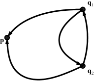
Figure 1: To $p$ via $q_{1}$ or via $q_{2}$

Corollary 1: In the case that $\mathcal{R}_{1}=\mathcal{R}\setminus\mathcal{R}_{2}$, namely when the junction graph decomposes into two junction trees (for example this can be the case when we choose a sub-tree in a graph with only one cycle), if $H(q_{1})\leq H(q_{2})$ the bound in (10) simplifies to

$$\mathcal{L}_{q_{2}}+D(q_{2}||q_{1})\;\leq\;\mathcal{L}_{q_{1}}+D(q_{1}||{q}_{2}).$$ (11)

Note that in general $D(\cdot||\cdot)$ is not symmetrical therefore equation (11) does not tell whether one bound is better than the other. According to (8) and the definition of $\mathcal{L}_{q_{T}}$, we can see that $\mathcal{L}_{q_{T}}=\ln(Z)-D(q_{T}||p)$ therefore we can rewrite (11) as

$$D(q_{2}||q_{1})+D(q_{1}||p)\;\leq\;D(q_{1}||q_{2})+D(q_{2}||p).$$ (12)

In other words, the distance from $q_{2}$ to $p$ via $q_{1}$ is shorter than the distance from $q_{1}$ to $p$ via $q_{2}$. See Fig. 1. Note that in general $D(\cdot||\cdot)$ does not satisfy the triangular inequality therefore equation (12) does not tell whether one bound is better than the other either.

Clearly, the distance from $q_{1}$ to $p$ is also shorter than the distance from $q_{1}$ to $p$ via $q_{2}$.

$$D(q_{1}||p)\;\leq\;D(q_{1}||q_{2})+D(q_{2}||p).$$ (13)

Corollary 2: Consider a subset $\mathcal{R}_{S}$ of $\mathcal{R}$ with junction tree representation. Also suppose that $q_{S}$, the probability distribution over $R_{S}$, has the smallest entropy among all the probability distributions on sub-trees. Then for any subset $\mathcal{R}_{T}$ of $\mathcal{R}$ with tree representation the following inequality holds

$$\mathcal{L}_{q_{T}}\,\leq\,\mathcal{L}_{q_{S}}\,+\,D(q_{S}||\overline{q}_{S}).$$ (14)

Proof:

According to Theorem 2

$$\mathcal{L}_{q_{T}}\leq\mathcal{L}_{q_{S}}+\\ \!\!\!\!\min\big{(}D(q_{S}||\overline{q}_{S})\!-\!D(q_{T}||q_{S}),\!D(q_{S}||q_{T})\!\!+\!\!D(q_{S}||\overline{q}_{T})\big{)}.$$

and hence the following

$$\mathcal{L}_{q_{T}} \leq \mathcal{L}_{q_{S}}\!+\!D(q_{S}||\overline{q}_{S})\!-\!D(q_{T}||q_{S})$$

$$\leq \mathcal{L}_{q_{S}}\!+\!D(q_{S}||\overline{q}_{S}).$$

∎

In other words, the lower bound obtained from any sub-tree can not be better than the lower bound obtained from the minimum entropy sub-tree by more than $D(q_{S}||\overline{q}_{S})$, a value that does not depend on $q_{T}$. This gives us a quality guarantee for the lower bound obtained from the minimum entropy sub-tree [7].

Theorem 3

Consider subsets $\mathcal{R}_{S}$ and $\mathcal{R}_{B}$ of $\mathcal{R}$ with junction tree representations. Also suppose that $q_{S}$, the probability distribution over $\mathcal{R}_{S}$, has the smallest entropy and $q_{B}$, the probability distribution over $\mathcal{R}_{B}$, gives the best lower bound, then the following inequality holds

$$D(q_{B}||q_{S})\,\leq\,D(q_{S}||\overline{q}_{S}).$$ (15)

Proof:

Since $H(q_{S})\leq H(q_{B})$ according to Theorem 2 we can write

$$\mathcal{L}_{q_{B}}\,\leq\,\mathcal{L}_{q_{S}}+D(q_{S}||\overline{q}_{S})-D(q_{B}||q_{S}).$$ (16)

Since $q_{B}$ gives the best lower bound

$$\mathcal{L}_{q_{S}}\,\leq\,\mathcal{L}_{q_{B}}.$$ (17)

The proof would be clear by adding equations (16) and (17). ∎

Theorem 3 gives us another quality guarantee regarding the minimum entropy sub-tree (which is the least random, least uncertain, and most biased sub-tree). This theorem shows that the probability distribution on the tree that gives the best bound and the minimum entropy distribution are close, where closeness is measured by divergence. The upper bound is $D(q_{S}||\overline{q}_{S})$ which does not depend on $q_{B}$ [7]. See Fig. 2.

Corollary 3: In the case that $\mathcal{R}_{S}=\mathcal{R}\setminus\mathcal{R}_{B}$ we have the following inequality

$$D(q_{B}||q_{S})\leq D(q_{S}||q_{B}).$$ (18)

remark 1: In almost all the theorems and corollaries, we insisted that the subsets of $\mathcal{R}$ have junction-tree representations. This assumption can be relaxed and the theorems and corollaries would still be valid for the sub-graphs. However, having a junction tree representation makes the computation of the entropy and the partition function easier (using GDL or any other iterative message passing algorithm).

Figure 2: Upper bound for divergence between $q_{B}$ and $q_{S}$

VI Conclusion

In this paper, we extended some of our previous results on bounding the partition function. In the case that the graph decomposes into two sub-trees we derived a number of divergence inequalities concerning the global probability distribution and the probability distributions on the sub-trees. We showed that the minimum entropy sub-tree has some optimality properties, namely the lower bound obtained from this tree can not be far from the lower bound obtained from any other sub-tree and the probability distribution on this tree and the probability distribution on the tree that gives the best lower bound are close where the divergence is the measure of closeness.

References

- [1] S. M. Aji and R. J. McEliece. “The Generalized Distributive Law,” IEEE Trans. Info. Theory, 325–343, March 2000.
- [2] S. M. Aji and R. J. McEliece. “The Generalized Distributive Law and Free Energy Minimization,” 39th Allerton Conference on Communication, Control, and Computing, October 2001.
- [3] M. Chertkov and V. Chernyak. “Loop Calculus in Statistical Physics and Information Science.” Phys. Rev. E 73, June 2006.
- [4] R. Cowell. Advanced Inference in Bayesian Networks. In Learning in Graphical Models. MIT Press, 1998.
- [5] M. Molkaraie and P. Pakzad. “On Entropy Decomposition and New Bounds on the Partition Function,” International Symposium on Info. Theory, Australia, September 2005.
- [6] M. Molkaraie and P. Pakzad. “Sub-tree Based Upper and Lower Bounds on the Partition Function,” International Symposium on Info. Theory, Seattle, July 2006.
- [7] M. Molkaraie, Subtree-Based Bounds and Simulation-Based Estimations for the Partition Function, Ph.D. dissertation , EPF Lausanne, Switzerland, 2007.
- [8] P. Pakzad and V. Anantharam. “Estimation and Marginalization Using Kikuchi Approximation Methods,” Neural Computation, 1836–1873, August 2005.
- [9] G. R. Shafer and P. P. Shenoy. “Probability Propagation,” Annals of Mathematics and Artificial Intelligence, 327–352, 1990.
- [10] M. J. Wainwright, T. Jaakkola, and A. S. Willsky. “A New Class of Upper Bounds on the Log Partition Function,” IEEE Trans. Info. Theory, 2313–2335, July 2005.
- [11] J. S. Yedidia, W. T. Freeman, and Y. Weiss. “Constructing Free Energy Approximations and Generalized Belief Propagation Algorithms,” IEEE Trans. Info. Theory, 2282–2312, July 2005.