Capillary instability in a two-component Bose–Einstein condensate

Abstract

Capillary instability and the resulting dynamics in an immiscible two-component Bose–Einstein condensate are investigated using the mean-field and Bogoliubov analyses. A long, cylindrical condensate surrounded by the other component is dynamically unstable against breakup into droplets due to the interfacial tension arising from the quantum pressure and interactions. A heteronuclear system confined in a cigar-shaped trap is proposed for realizing this phenomenon experimentally.

I Introduction

A fluid cylinder will be unstable against breakup into droplets if its length exceeds its circumference. A familiar example is a water jet projected into air, which breaks up into many water droplets. Savart Savart first investigated this kind of instability and Plateau Plateau subsequently developed an experimental technique. Lord Rayleigh Rayleigh used linear stability analysis to investigate this phenomenon. This instability is known as capillary instability Chandra (or sometimes as Plateau–Rayleigh instability). The present paper proposes a method for observing capillary instability in quantum degenerate gases.

Classical fluid instabilities have recently been studied theoretically in quantum fluids with renewed interest. Various fluid instabilities are predicted to be observable in two-component Bose–Einstein condensates (BECs) including the Rayleigh–Taylor instability Sasaki ; Gautam , the Kelvin–Helmholtz instability Takeuchi ; Suzuki , the Richtmyer–Meshkov instability Bezett , the counter-superflow instability Law ; TakeuchiL , and the Rosensweig instability SaitoL . Of these, the counter-superflow instability has recently been realized experimentally Hoefer . The Bénard–von Kármán vortex street, which is predicted to occur in single-component SasakiL and two-component BECs Sasaki2 , is also caused by fluid instability.

In the present paper, we investigate capillary instability and the resulting dynamics in a two-component BEC. Capillary instability in a water jet originates from the surface tension of water that results from the attractive interaction between water molecules. By contrast, in the present study, we demonstrate that capillary instability emerges in an atomic gas with repulsive inter- and intra-atomic interactions. We consider an immiscible two-component BEC in which a cylinder of component 1 is surrounded by component 2. The interfacial tension between the two components Barankov ; Schae induces capillary instability and component 1 breaks into droplets that form a matter-wave soliton train. This system thus exhibits capillary instability and is novel in that the instability is only due to repulsive interactions. We also demonstrate that dark–bright soliton and skyrmion trains can be generated in this system.

The present paper is organized as follows. Section II numerically demonstrates capillary instability and subsequent dynamics in an ideal system. Section III examines the stability of the system using Bogoliubov and linear stability analyses. Section IV proposes a realistic system for observing capillary instability in a trapped two-component BEC and numerically demonstrates various dynamics. Section V presents the conclusions of this study.

II Dynamics in an ideal system

We consider a two-component BEC of atoms with mass $m_{j}$ in an external potential $V_{j}$, where the subscript $j=1$, $2$ indicates component 1 or 2. In zero-temperature mean-field theory, the macroscopic wave functions $\psi_{1}$ and $\psi_{2}$ obey the Gross–Pitaevskii (GP) equation given by

$$i\hbar\frac{\partial\psi_{1}}{\partial t} = \left(-\frac{\hbar^{2}}{2m_{1}}\nabla^{2}+V_{1}+g_{11}|\psi_{1}|^{2}+g_{12}|\psi_{2}|^{2}\right)\psi_{1},$$

$$i\hbar\frac{\partial\psi_{2}}{\partial t} = \left(-\frac{\hbar^{2}}{2m_{2}}\nabla^{2}+V_{2}+g_{22}|\psi_{2}|^{2}+g_{12}|\psi_{1}|^{2}\right)\psi_{2},$$

where the interaction parameters are defined as

$$g_{jj^{\prime}}=2\pi\hbar^{2}a_{jj^{\prime}}\left(m_{j}^{-1}+m_{j^{\prime}}^{-1}\right),$$ (2)

with $a_{jj^{\prime}}$ being the $s$-wave scattering length between the atoms in components $j$ and $j^{\prime}$ $(j,j^{\prime}=1,2)$. We assume that the interaction parameters satisfy

$$g_{11}g_{22}<g_{12}^{2},$$ (3)

for which the two components are immiscible Pethick .

In this section, we consider an ideal system with $V_{1}=V_{2}=0$, $m_{1}=m_{2}\equiv m$, and $g_{11}=g_{22}\equiv g$. Normalizing the length and time in Eq. (1) by $\xi=\hbar/(mgn)^{1/2}$ and $\xi/v_{\rm s}$, where $n$ is the atomic density $|\psi_{2}|^{2}$ far from the interface and $v_{\rm s}=(gn/m)^{1/2}$ is the sound velocity, we find that the intracomponent interaction coefficients are normalized to unity and the relevant parameter is only $g_{12}/g$. The initial state is a stationary state $\Psi_{j}(r)$ in which component 1 is a cylinder centered about the $z$ axis and is surrounded by component 2. The state $\Psi_{j}(r)$ depends only on $r=(x^{2}+y^{2})^{1/2}$ and has cylindrical symmetry and translation symmetry along $z$. Numerically, this initial state is prepared by imaginary time propagation of the GP equation (1). The time evolution of the system is obtained by numerically solving the GP equation (1) by the pseudospectral method.

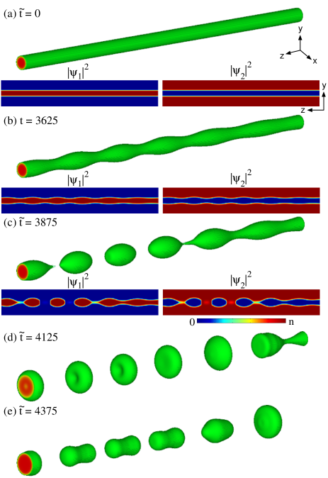
Figure 1: (Color online) Capillary instability and resulting dynamics of a two-component BEC for $g_{12}/g=1.1$. The three-dimensional objects depict the isodensity surface of component 1. The lower panels in (a)–(c) show the density distributions $|\psi_{j}|^{2}$ at the cross section of $x=0$ (the field of view is $600\xi\times 100\xi$). The number of component 1 atoms in an initial cylinder with length $\xi$ is $N_{1\xi}=400$.

Figure 1 shows the time evolution of the system for $g_{12}/g=1.1$, where the number of component 1 atoms in an initial cylinder with length $\xi$,

$$N_{1\xi}\equiv\xi\int dxdy|\Psi_{1}|^{2},$$ (4)

is 400. We add a small white noise to the initial state to break the exact numerical symmetry. At $\tilde{t}\equiv tv_{\rm s}/\xi=3600$, “varicose” Chandra modulation with a wavelength $\simeq 99\xi\simeq 9.0R_{0}$ occurs on the cylindrical interface [Fig. 1 (b)], where $R_{0}$ is the initial radius of the cylinder of component 1. The varicosities then split into droplets [Fig. 1 (c)], which undergo quadrupole oscillations [Figs. 1 (d) and 1 (e)] due to the kinetic energy converted from the interfacial tension energy. The droplets subsequently aggregate to minimize the interfacial tension energy.

Figure 2: (Color online) Time evolution of the system with a periodic initial perturbation given by Eq. (5). The parameters are the same as those in Fig. 1. The three-dimensional objects indicate the isodensity surfaces of component 1 and the lower panels show the density distributions $|\psi_{j}|^{2}$ at the cross section of $x=0$ (the field of view is $600\xi\times 100\xi$).

Figure 2 shows the time evolution of the system, where a periodic initial perturbation is added to component 1 as

$$\Psi_{1}(r)\left(1+0.01\cos\frac{2\pi z}{200\xi}\right),$$ (5)

instead of the white noise. This wavelength $200\xi$ is about twice the most unstable wavelength in the modulation in Fig. 1 (b). The sinusoidal seed develops into a highly nonlinear pattern [Fig. 2 (a)] and the thin ligaments separate from the main droplets [Fig. 2 (b)], which deform into small drops [Fig. 2 (c)]. Such nonlinear behavior is very similar to that in classical liquid jets Bogy , and the small drops are termed “satellite drops”.

III Stability analysis

III.1 Bogoliubov analysis

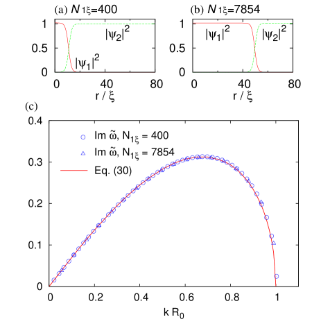
Figure 3: (Color online) Radial density profiles of the stationary states for (a) $N_{1\xi}=400$ and (b) $N_{1\xi}=7854$ with $g_{12}/g=1.1$. (c) Imaginary part of the excitation frequencies. The circles and triangles are obtained by numerical diagonalization of Eq. (9) with the parameters used in (a) and (b), respectively. The plotted quantities are normalized using Eq. (10) with $R_{0}=11\xi$ for the circles and $R_{0}=50\xi$ for the triangles. The solid curve indicates Eq. (30).

We study the stability of an ideal system such as that depicted in Fig. 1 (a) using Bogoliubov theory. We separate the wave function as

$$\psi_{j}(r,z,t)=\left[\Psi_{j}(r)+\delta\psi_{j}(r,z,t)\right]e^{-i\mu_{j}t/\hbar},$$ (6)

where $\mu_{j}$ is the chemical potential and the system is assumed to have cylindrical symmetry. Figures 3 (a) and 3 (b) show examples of the stationary state $\Psi_{j}(r)$. Substituting Eq. (6) into the GP equation (1) and taking the first order of the small deviation $\delta\psi_{j}$, we find $(j\neq j^{\prime})$

$$i\hbar\frac{\partial\delta\psi_{j}}{\partial t} = \left(-\frac{\hbar^{2}}{2m_{j}}\nabla^{2}+V_{j}-\mu_{j}+2g_{jj}\Psi_{j}^{2}+g_{jj^{\prime}}\Psi_{j^{\prime}}^{2}\right)\delta\psi_{j}$$ (7)

$$+g_{jj}\Psi_{j}^{2}\delta\psi_{j}^{*}+g_{jj^{\prime}}\Psi_{j}\Psi_{j^{\prime}}(\delta\psi_{j^{\prime}}+\delta\psi_{j^{\prime}}^{*}),$$

where $\Psi_{1}$ and $\Psi_{2}$ are assumed to be real without loss of generality. Using the excitation mode of the form

$$\delta\psi_{j}=u_{jk}(r)e^{i(kz-\omega t)}+v_{jk}^{*}(r)e^{-i(kz-\omega t)}$$ (8)

in Eq. (7), we obtain the Bogoliubov–de Gennes equation $(j\neq j^{\prime})$,

$$\left[-\frac{\hbar^{2}}{2m_{j}}\left(\frac{\partial^{2}}{\partial r^{2}}+\frac{1}{r}\frac{\partial}{\partial r}-k^{2}\right)+V_{j}-\mu_{j}+2g_{jj}\Psi_{j}^{2}+g_{jj^{\prime}}\Psi_{j^{\prime}}^{2}\right]u_{jk}+g_{jj}\Psi_{j}^{2}v_{jk}+g_{jj^{\prime}}\Psi_{j}\Psi_{j^{\prime}}(u_{j^{\prime}k}+v_{j^{\prime}k}) = \hbar\omega u_{jk},$$ (9a)

$$\left[-\frac{\hbar^{2}}{2m_{j}}\left(\frac{\partial^{2}}{\partial r^{2}}+\frac{1}{r}\frac{\partial}{\partial r}-k^{2}\right)+V_{j}-\mu_{j}+2g_{jj}\Psi_{j}^{2}+g_{jj^{\prime}}\Psi_{j^{\prime}}^{2}\right]v_{jk}+g_{jj}\Psi_{j}^{2}u_{jk}+g_{jj^{\prime}}\Psi_{j}\Psi_{j^{\prime}}(u_{j^{\prime}k}+v_{j^{\prime}k}) = -\hbar\omega v_{jk}.$$ (9b)

Figure 3 (c) shows the imaginary part of the Bogoliubov excitation frequency obtained by numerical diagonalization of Eq. (9). For comparison with an analytic result given in the next subsection, we plot the normalized quantity as

$${\rm Im}\tilde{\omega}\equiv\sqrt{\frac{mnR_{0}^{3}}{\alpha}}{\rm Im}\omega,$$ (10)

where $\alpha$ is the interfacial tension coefficient originating from the excess kinetic and interaction energies at the interface. For $g_{12}/g=1.1$, we can use the expression for the interfacial tension coefficient obtained in Refs. Barankov ; Schae , namely,

$$\alpha=\frac{\hbar n^{3/2}}{\sqrt{2m}}\sqrt{g_{12}-g}.$$ (11)

Figure 3 (c) reveals that the most unstable wavelength is $\simeq 9.3R_{0}$, which agrees with the modulation in Fig. 1 (b). In Fig. 3 (c), we plot two cases for the parameters corresponding to Fig. 3 (a) (circles) and Fig. 3 (b) (triangles). We note that these plots fall on a universal curve using the scaling in Eq. (10).

III.2 Linear stability analysis

To understand the Bogoliubov spectrum obtained in Fig. 3, we analyze the stability of the system using a similar method to Rayleigh’s linear stability analysis Rayleigh ; Chandra . We start from the mean-field Lagrangian given by

$$L=\int d\bm{r}\left(P_{1}+P_{2}-g_{12}|\psi_{1}|^{2}|\psi_{2}|^{2}\right),$$ (12)

where

$$P_{j}=i\hbar\psi_{j}^{*}\frac{\partial\psi_{j}}{\partial t}-\frac{\hbar^{2}}{2m_{j}}|\bm{\nabla}\psi_{j}|^{2}-V_{j}|\psi_{j}|^{2}-\frac{g_{jj}}{2}|\psi_{j}|^{4}.$$ (13)

The functional derivative of the action $\int Ldt$ with respect to $\psi_{j}^{*}$ gives the GP equation (1). In this subsection, we assume that the two components are strongly phase separated and that the interface thickness is negligibly small. We also assume that the system has cylindrical symmetry and that the interface is located at $r=R(z,t)$. We then approximate Eq. (12) as

$$L=2\pi\int dz\left(\int_{0}^{R}rdrP_{1}+\int_{R}^{\infty}rdrP_{2}\right)-\alpha S,$$ (14)

where $S$ is the area of the interface. Differentiating Eq (14) with respect to $R$, we obtain Landau

$$P_{1}(R,z,t)-P_{2}(R,z,t)=\alpha\left(\frac{1}{R_{1}}+\frac{1}{R_{2}}\right),$$ (15)

where $R_{1}$ and $R_{2}$ are the principal radii of the interface curvature. Equation (15) corresponds to Laplace’s formula in fluid mechanics.

We write the wave function as

$$\psi_{j}(r,z,t)=\sqrt{n_{j}(r,z,t)}e^{i\phi_{j}(r,z,t)},$$ (16)

where $n_{j}$ and $\phi_{j}$ are real functions, $n_{1}=0$ for $r>R$, and $n_{2}=0$ for $r<R$. We separate the density and phase as

$$n_{j}(r,z,t) = n_{j0}+\delta n_{j}(r,z,t),$$ (17a)

$$\phi_{j}(r,z,t) = -\frac{g_{jj}n_{j0}}{\hbar}t+\delta\phi_{j}(r,z,t),$$ (17b)

and substitute them into Eq. (1). Taking the first order of $\delta\phi_{j}$ and $g_{jj}\delta n_{j}$, we have

$$\bm{\nabla}\cdot\bm{v}_{j} = 0,$$ (18)

$$\hbar\frac{\partial\delta\phi_{j}}{\partial t}+g_{jj}\delta n_{j} = 0,$$ (19)

where the velocity is defined as

$$\bm{v}_{j}=\frac{\hbar}{m_{j}}\bm{\nabla}\delta\phi_{j}.$$ (20)

The gradient of Eq. (19) gives

$$m_{j}\frac{\partial\bm{v}_{j}}{\partial t}+g_{jj}\bm{\nabla}\delta n_{j}=0.$$ (21)

Substituting Eq. (17) into Eq. (13) and using Eq. (19), we obtain the pressure,

$$P_{j}=\frac{1}{2}g_{jj}n_{j0}^{2}+g_{jj}n_{j0}\delta n_{j}.$$ (22)

We assume the sinusoidal forms of the small excitation as

$$R(z,t) = R_{0}+\epsilon\sin(kz-\omega t),$$ (23a)

$$v_{jr}(r,z,t) = \tilde{v}_{jr}(r)\cos(kz-\omega t),$$ (23b)

$$v_{jz}(r,z,t) = \tilde{v}_{jz}(r)\sin(kz-\omega t),$$ (23c)

$$\delta n_{j} = \delta\tilde{n}_{j}(r)\sin(kz-\omega t).$$ (23d)

Using Eqs. (22) and (23), Eq. (15) becomes

$$g_{11}n_{10}\delta\tilde{n}_{1}(r)-g_{22}n_{20}\delta\tilde{n}_{2}(r)=\frac{\alpha\epsilon}{R_{0}^{2}}(k^{2}R_{0}^{2}-1),$$ (24)

where we have used the equilibrium condition $(g_{11}n_{10}^{2}-g_{22}n_{20}^{2})/2=\alpha/R_{0}$. Substituting Eqs. (23b)–(23d) into Eqs. (18) and (21) yields

$$r^{2}\tilde{v}_{jr}^{\prime\prime}(r)+r\tilde{v}_{jr}^{\prime}(r)-(1+k^{2}r^{2})\tilde{v}_{jr}(r)=0.$$ (25)

The solutions of this differential equation are

$$\tilde{v}_{1r}(r) = c_{1}I_{1}(kr),$$ (26a)

$$\tilde{v}_{2r}(r) = c_{2}K_{1}(kr),$$ (26b)

where $c_{1}$ and $c_{2}$ are constants and $I_{n}$ and $K_{n}$ are modified Bessel functions of the first and second kinds. These functions are chosen such that components 1 and 2 do not diverge at the $z$ axis and infinity, respectively. It follows from Eqs. (21) and (26) that

$$g_{11}\delta\tilde{n}_{1}(r) = -\frac{m_{1}\omega c_{1}}{k}I_{0}(kr),$$ (27a)

$$g_{22}\delta\tilde{n}_{2}(r) = \frac{m_{2}\omega c_{2}}{k}K_{0}(kr).$$ (27b)

The kinematic boundary condition at the interface is $dR/dt=v_{1r}(R)=v_{2r}(R)$, which gives

$$\epsilon\omega=-c_{1}I_{1}(R_{0})=-c_{2}K_{1}(R_{0}).$$ (28)

Using Eqs. (24), (27), and (28), we obtain the dispersion relation of the excitation as

$$\omega^{2}=\frac{\alpha}{R_{0}^{3}}\frac{kR_{0}(k^{2}R_{0}^{2}-1)}{m_{1}n_{10}\frac{I_{0}(kR_{0})}{I_{1}(kR_{0})}+m_{2}n_{20}\frac{K_{0}(kR_{0})}{K_{1}(kR_{0})}}.$$ (29)

This dispersion relation has the same form as that of classical inviscid incompressible fluids Chris . The quantum mechanical pressure is included in the interfacial tension coefficient $\alpha$ and Eq. (29) does not contain any explicit quantum correction term. For $0<kR_{0}<1$, the right-hand side of Eq. (29) is negative and the frequency $\omega$ is pure imaginary. The mode with a wavelength larger than $2\pi R_{0}$ is therefore dynamically unstable. The most unstable wave number is given by $kR_{0}\simeq 0.68$ and the most unstable wavelength is $\simeq 9.2R_{0}$, which is in good agreement with the modulation wavelength in Fig. 1 (b). The most unstable wave number depends only on $R_{0}$ and is independent of the interaction parameters. The interaction, which is included in $\alpha$, only affects the growth rate of the unstable modes.

The solid line in Fig. 3 indicates

$$\sqrt{\frac{mnR_{0}^{3}}{\alpha}}{\rm Im}\omega=\sqrt{\frac{kR_{0}(1-k^{2}R_{0}^{2})}{\frac{I_{0}(kR_{0})}{I_{1}(kR_{0})}+\frac{K_{0}(kR_{0})}{K_{1}(kR_{0})}}}$$ (30)

for $0<kR_{0}<1$, which is in excellent agreement with the numerically obtained Bogoliubov spectrum normalized by Eq. (10). This confirms that the modulation instability shown in Fig. 1 (b) is the capillary instability. Figure 3 shows that the dispersion relation (29) is accurate even when the radius of the cylinder of component 1 is of the same order as the interface thickness.

IV Dynamics in a trapped system

We propose a realistic experimental situation to observe the capillary instability in a trapped BEC. We consider a heteronuclear condensate consisting of ${}^{41}{\rm K}$ (component 1) and ${}^{87}{\rm Rb}$ (component 2) atoms in the stretched $|F=2,m_{F}=2\rangle$ states. Modugno . The scattering lengths are $a_{11}=65a_{\rm B}$ Wang , $a_{22}=99a_{\rm B}$ Marte , and $a_{12}=163a_{\rm B}$ Ferlaino , which satisfy the phase separation condition in Eq. (3). The two components are confined in axisymmetric harmonic potentials,

$$V_{j}=\frac{m_{j}}{2}(\omega_{j\perp}^{2}r^{2}+\omega_{jz}^{2}z^{2}),$$ (31)

produced by laser beams. Since the electronic excitation frequencies of the two atomic species are separated from each other, $V_{1}$ and $V_{2}$ can be chosen independently by using laser beams with different frequencies.

The initial state is prepared for trap frequencies satisfying $\omega_{1\perp}\gg\omega_{2\perp}$ and $\omega_{j\perp}\gg\omega_{jz}$. Since the radial confinement of component 1 is much tighter than that of component 2, the ground state of component 1 is extremely narrow and it is surrounded by component 2 in the radial direction. The tight radial confinement prevents component 1 from breaking up into droplets for the same reason as why a classical liquid in a pipe never exhibits the capillary instability. We then add small white noise to the initial state and reduce $\omega_{1\perp}$ suddenly at $t=0$. This produces an unstable initial state similar to the state in Fig. 1 (a), and capillary instability is obtained.

Figure 4: (Color online) Time evolution of a ${}^{41}{\rm K}$-${}^{87}{\rm Rb}$ condensate confined in a cigar-shaped trap. The initial state is the ground state, in which $N_{1}=5\times 10^{4}$ ${}^{41}{\rm K}$ atoms (component 1) are confined in $V_{1}$ with $(\omega_{1\perp},\omega_{1z})/2\pi=(582,11.6)$ Hz and $N_{2}=9.5\times 10^{5}$ ${}^{87}{\rm Rb}$ atoms (component 2) are confined in $V_{2}$ with $(\omega_{2\perp},\omega_{2z})/2\pi=(89.4,7.2)$ Hz. At $t=0$, $\omega_{1\perp}/(2\pi)$ is changed from $582$ Hz to $145$ Hz. The panels in (a)–(c) show the density distributions $|\psi_{j}|^{2}$ at the cross section of $x=0$, where the unit of the density is $10^{20}$ ${\rm m}^{-3}$ and the field of view is $220\times 14$ $\mu{\rm m}$. The bottom figure shows the isodensity surface of component 1 at $t=21$ ms.

Figure 4 demonstrates the capillary instability and resulting dynamics of a trapped two-component BEC obtained by numerically solving the 3D GP equation. The ratio of the number of atoms in component 1 to the total number of atoms is $N_{1}/(N_{1}+N_{2})=0.05$. At $t=0$, the radial confinement of component 1 is relaxed and modulation grows due to the capillary instability. Varicose modulation occurs in component 1 [Fig. 4 (b)], which breaks up into droplets [Fig. 4 (c)]. The axisymmetry of the system is preserved within this time scale. We have thus shown that the capillary instability can be observed in a trapped two-component BEC. The structure in Fig. 4 (c) is similar to a matter-wave soliton train. A matter-wave soliton and soliton train have so far been produced by a single-component BEC with attractive interactions Khay ; Strecker . By contrast, the train of matter-wave droplets in Fig. 4 (c) is produced only by repulsive interactions.

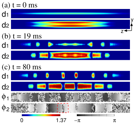
Figure 5: (Color online) Time evolution for $N_{1}=2\times 10^{5}$ and $N_{2}=8\times 10^{5}$. The trap frequencies are $(\omega_{1\perp},\omega_{1z})/2\pi=(436,35)$ and $(\omega_{2\perp},\omega_{2z})/2\pi=(89.4,7.2)$. At $t=0$, $\omega_{1\perp}/2\pi$ is changed to 145 Hz. The panels show the column density $d_{j}=\int|\psi_{j}|^{2}dx$ and the phase $\phi_{j}={\rm arg}\psi_{j}(x=0)$. The unit of the column density is $10^{15}$ ${\rm m}^{-2}$ and the field of view is $170\times 13.6$ $\mu{\rm m}$. The dashed square in (c) shows an example of a position at which the phase jumps.

Figure 5 shows the dynamics for $N_{1}/(N_{1}+N_{2})=0.2$. Since the radius of the initial cylinder of component 1 is larger than that in Fig. 4, the modulation wavelength for the capillary instability is larger. The size of each droplet produced by the capillary instability is thus larger than that in Fig. 4 and the droplets cut component 2 along the $z$ axis [Fig. 5 (c)]. The two-component structure in Fig. 5 (c) is similar to dark–bright solitons Busch ; Becker ; Hamner , where the density dips in component 2 and the droplets of component 1 correspond to dark and bright solitons, respectively. In fact, the phase $\phi_{2}$ of component 2 jumps at the density dips [dashed square in Fig. 5 (c)], which is required to stabilize dark–bright solitons.

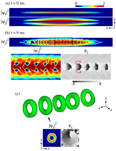
Figure 6: (Color online) Creation of a skyrmion train. (a) Density distribution of the initial state at the cross section of $x=0$. Component 1 has a singly quantized vortex along the $z$ axis. The initial trap frequencies for component 1 are $(\omega_{1\perp},\omega_{1z})/2\pi=(796,14.5)$ Hz. At $t=0$, $\omega_{1\perp}$ is changed to 145 Hz and the trap center for component 1 is shifted to $z=65$ $\mu{\rm m}$. The other parameters are the same as those in Fig. 4. The field of view is $150\times 14$ $\mu{\rm m}$. (b) Density profile of component 2 at the cross section of $x=0$ at $t=9$ ms. The density and phase in the dashed square are magnified in the lower panels. The arrows indicate the directions of circulations of the quantized vortices. (c) Isodensity surface of component 1 at $t=9$ ms. The lower panels show the density and phase profiles of component 1 at the cross section of $z$ indicated by the arrow. The unit of the density in (a)–(c) is $10^{20}$ ${\rm m}^{-3}$.

Figure 6 demonstrates generation of a skyrmion train using the capillary instability. The initial state is a stationary state in which component 1 has a singly quantized vortex line along the $z$ axis [Fig. 6 (a)]. Such a state is generated by phase imprinting using, for example, a stimulated Raman transition with Laguerre–Gaussian beams Andersen . At $t=0$, the radial confinement of component 1 is reduced and a force in the $z$ direction is exerted on component 1; this can be achieved, for example, by shifting the trap center in the $z$ direction. Figures 6 (b) and 6 (c) show the state at $t=9$ ms. The isodensity surface in Fig. 6 (c) indicates that the initial hollow cylinder of component 1 breaks up into toruses due to the capillary instability. The initial vortex remains in component 1, as shown in Fig. 6 (d). This breakup is not due to the Kelvin–Helmholtz instability since it occurs in a very similar manner when there is no force in the $z$ direction. The vortex rings are generated in component 2 [Fig. 6 (b)] at locations where there are toruses of component. This vortex ring generation is due to the acceleration of the toruses of component 1 in the $z$ direction Sasaki2 . The structures produced in Fig. 6 are thus the skyrmions in a two-component BEC Ruo . However, the skyrmion train in Fig. 6 is unstable against axisymmetry breaking. Because of the vortex quantization, the behavior in Fig. 6 is quite different from that in an axially rotating jet of a classical fluid Rutland .

V Conclusions

We have investigated the capillary instability and resulting dynamics in a two-component BEC. We first demonstrated the dynamics in an ideal system in Sec. II. We have shown that modulation occurs on a cylinder of component 1 due to the capillary instability and the cylinder breaks up into droplets (Fig. 1), as in a classical fluid jet. Formation of satellite drops was also observed (Fig. 2). In Sec. III, we performed Bogoliubov analysis and numerically obtained a dynamically unstable spectrum, which is in good agreement with that obtained by Rayleigh’s linear stability analysis (Fig. 3). In Sec. IV, we proposed realistic trapped systems and numerically demonstrated the dynamics caused by the capillary instability. We have shown that the capillary instability can be observed in a heteronuclear two-component BEC confined in a cigar-shaped harmonic trap, where the radial confinement of inner component is controlled (Fig. 4). We have also shown that dark–bright soliton and skyrmion trains can be generated in this system, which are quantum mechanical objects and have no counterparts in capillary instability in classical fluids.

- (1) F. Savart, Ann. Chim. Phys. 53, 337 (1833).
- (2) J. Plateau, Acad. Sci. Bruxelles M’em. 16, 3 (1843); ibid. 23, 5 (1849).
- (3) Lord Rayleigh, Proc. London Math. Soc. 10, 4 (1878).
- (4) See, e.g., S. Chandrasekhar, Hydrodynamic and hydromagnetic stability, Chap XII, (Oxford Univ. Press, 1961, London).
- (5) K. Sasaki, N. Suzuki, D. Akamatsu, and H. Saito, Phys. Rev. A 80, 063611 (2009).
- (6) S. Gautam and D. Angom, Phys. Rev. A 81, 053616 (2010).
- (7) H. Takeuchi, N. Suzuki, K. Kasamatsu, H. Saito, and M. Tsubota, Phys. Rev. B 81, 094517 (2010).
- (8) N. Suzuki, H. Takeuchi, K. Kasamatsu, M. Tsubota, and H. Saito, Phys. Rev. A 82, 063604 (2010).
- (9) A. Bezett, V. Bychkov, E. Lundh, D. Kobyakov, and M. Marklund, Phys. Rev. A 82, 043608 (2010).
- (10) C. K. Law, C. M. Chan, P. T. Leung, and M.-C. Chu, Phys. Rev. A 63, 063612 (2001).
- (11) H. Takeuchi, S. Ishino, and M. Tsubota, Phys. Rev. Lett. 105, 205301 (2010).
- (12) H. Saito, Y. Kawaguchi, and M. Ueda, Phys. Rev. Lett. 102, 230403 (2009).
- (13) M. A. Hoefer, C. Hamner, J. J. Chang, and P. Engels, e-print arXiv:1007.4947.
- (14) K. Sasaki, N. Suzuki, and H. Saito, Phys. Rev. Lett. 104, 150404 (2010).
- (15) K. Sasaki, N. Suzuki, and H. Saito, to be published in Phys. Rev. A.
- (16) R. A. Barankov, Phys. Rev. A 66, 013612 (2002).
- (17) B. Van Schaeybroeck, Phys. Rev. A 78, 023624 (2008); 80, 065601 (2009).
- (18) C. J. Pethick and H. Smith, Bose–Einstein Condensation in Dilute Gases, 2nd ed., Chap. 12, (Cambridge University Press, Cambridge, 2008).
- (19) For review, see for example, D. B. Bogy, Ann. Rev. Fluid Mech. 11, 207 (1979).
- (20) L. D. Landau and E. M. Lifshitz, Fluid Mechanics, 2nd ed., Chap. VII, (Butterworth-Heinemann, Oxford, 1987).
- (21) R. M. Christiansen and A. N. Hixson, Ind. Eng. Chem. 49, 1017 (1957).
- (22) G. Modugno, M. Modugno, F. Riboli, G. Roati, and M. Inguscio, Phys. Rev. Lett. 89, 190404 (2002).
- (23) H. Wang, A. N. Nikolov, J. R. Ensher, P. L. Gould, E. E. Eyler, W. C. Stwalley, J. P. Burke, Jr., J. L. Bohn, C. H. Greene, E. Tiesinga, C. J. Williams, and P. S. Julienne, Phys. Rev. A 62, 052704 (2000).
- (24) A. Marte, T. Volz, J. Schuster, S. Dürr, G. Rempe, E. G. M. van Kempen, and B. J. Verhaar, Phys. Rev. Lett. 89, 283202 (2002).
- (25) F. Ferlaino, C. D’Errico, G. Roati, M. Zaccanti, M. Inguscio, G. Modugno, and A. Simoni, Phys. Rev. A 73, 040702(R) (2006); 74, 039903(E) (2006).
- (26) L. Khaykovich, F. Schreck, G. Ferrari, T. Bourdel, J. Cubizolles, L. D. Carr, Y. Castin, and C. Salomon, Science 296, 1290 (2002).
- (27) K. E. Strecker, G. B. Partridge, A. G. Truscott, and R. G. Hulet, Nature (London) 417, 150 (2002).
- (28) Th. Busch and J. R. Anglin, Phys. Rev. Lett. 87, 010401 (2001).
- (29) C. Becker, S. Stellmer, P. Soltan-Panahi, S. Dörscher, M. Baumert, E. -M. Richter, J. Kronjäger, K. Bongs, and K. Sengstock, Nature Phys. 4, 496 (2008).
- (30) C. Hamner, J. J. Chang, P. Engels, and M. A. Hoefer, Phys. Rev. Lett. 106, 065302 (2011).
- (31) M. F. Andersen, C. Ryu, P. Cladé, V. Natarajan, A. Vaziri, K. Helmerson, and W. D. Phillips, Phys. Rev. Lett. 97, 170406 (2006).
- (32) J. Ruostekoski and J. R. Anglin, Phys. Rev. Lett. 86, 3934 (2001).
- (33) D. F. Rutland and G. J. Jameson, Chem. Eng. Sci. 25, 1301 (1970).