Interaction of oblique dark solitons in two-dimensional supersonic nonlinear Schrödinger flow

Abstract

We investigate the collision of two oblique dark solitons in the two-dimensional supersonic nonlinear Schrödinger flow past two impenetrable obstacles. We numerically show that this collision is very similar to the dark solitons collision in the one dimensional case. We observe that it is practically elastic and we measure the shifts of the solitons positions after their interaction.

1. Two-dimensional (2D) oblique dark solitons are unstable with respect to transverse perturbations kp-1970 ; zakharov-1975 ; kt-1988 and therefore their interaction with each other is not of much interest from practical point of view. However, it has been found egk-06 that such solitons generated in the flow of an atomic Bose-Einstein condensate (BEC) past an obstacle behave as effectively stable. Such a behavior was explained in kp-08 as a result of the transition from absolute instability of 2D solitons to their convective instability for large enough velocities of the flow in the reference frame attached to the obstacle, so that unstable modes are convected by the flow along the solitons from the region around the obstacle. The condition for convective instability of these dark solitons was derived in kk-11 . This phenomenon has a general nature and its nonlinear optics counterpart has been discussed in kgegk-08 . Recently, experimental observations in Bose-Einstein condensate of exciton-polaritons have indeed demonstrated the existence of stable oblique dark solitons in a superfluid flow past an obstacle amo-2010 . Hence, interaction of such effectively stable oblique dark solitons becomes a question of considerable interest and it will be addressed in this paper.

2. Oblique dark solitons in a superfluid are described very well egk-06 as stationary solutions of the defocusing nonlinear Schrödinger equation (NLS)

$$i\psi_{t}=-\frac{1}{2}\Delta\psi+|\psi|^{2}\psi\,,$$ (1)

which is written here in standard dimensionless units and $\Delta\equiv\partial^{2}_{x}+\partial^{2}_{y}$. Its transformation to a “hydrodynamic form” by means of the substitution

$$\psi({\bf r},t)=\sqrt{n({\bf r},t)}\exp\left(i\int^{{\bf r}^{\prime}}{\bf u}({\bf r}^{\prime},t)d{\bf r}^{\prime}\right)$$ (2)

yields the system

$$n_{t}+\nabla\cdot(n{\bf u})=0,$$ (3)

$${\bf u}_{t}+({\bf u}\cdot\nabla){\bf u}+\nabla n+\nabla\left(\frac{(\nabla n)^{2}}{8n^{2}}-\frac{\Delta n}{4n}\right)=0,$$ (4)

where $n$ is the density of the fluid and ${\bf u}$ denotes its velocity field.

In a stationary case $(n_{t}=0,\,{\bf u}_{t}=0)$ this system takes the form

$$\begin{split}(nu)_{x}+(nv)_{y}=0,\\ uu_{x}+vu_{y}+n_{x}+\left(\frac{n_{x}^{2}+n_{y}^{2}}{8n^{2}}-\frac{n_{xx}+n_{yy}}{4n}\right)_{x}=0,\\ uv_{x}+vv_{y}+n_{y}+\left(\frac{n_{x}^{2}+n_{y}^{2}}{8n^{2}}-\frac{n_{xx}+n_{yy}}{4n}\right)_{y}=0,\end{split}$$ (5)

where we have introduced the components ${\bf u}=(u,v)$ of the velocity field. It should be solved with the boundary conditions

$$n=1,\quad u=M,\quad v=0\quad\text{at}\quad|x|\to\infty,$$ (6)

which means that there is a uniform flow of a superfluid with constant velocity ${\bf u}=(M,0)$ at infinity. Since in our dimensionless units the sound velocity at infinity is equal to unity, the incoming velocity coincides with the Mach number $M$. The soliton solution of this problem was found in egk-06 and it can be written as

$$n(x,y)=1-\frac{1-M^{2}\sin^{2}\theta}{\cosh^{2}[\sqrt{1-M^{2}\sin^{2}\theta}(x\sin\theta-y\cos\theta+y_{0}\cos\theta)]},$$ (7)

$$u(x,y)=M\left[1+\sin^{2}\theta\left(\frac{1}{n(x,y)}-1\right)\right],\quad v(x,y)=-M\sin\theta\cos\theta\left(\frac{1}{n(x,y)}-1\right),$$ (8)

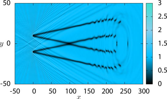
Figure 1: Interaction of two oblique dark solitons generated in the flow of a superfluid past two impenetrable obstacles. The flow is from the left to the right with $M=5$. One obstacle is located at $(x_{10},y_{10})=(0,-10)$ and the other one at $(x_{20},y_{20})=(0,10)$ . Colors indicate the magnitude of the density.

where $\theta$ is the angle between the oblique soliton and the horizontal axis and $y_{0}$ is its intersection point with the $y$ axis. The transformation (2) implies that the flow is potential (vorticity free) so that the velocity field u can be represented as a gradient of the phase

$$\phi(x,y)=Mx-\arctan\frac{M\sin\theta}{\sqrt{1-M^{2}\sin^{2}\theta}\tanh[\sqrt{1-M^{2}\sin^{2}\theta}(x\sin\theta-y\cos\theta+y_{0}\cos\theta)]}.$$ (9)

Correspondingly, the wave function of the oblique soliton reads

$$\psi(x,y)=\left\{\sqrt{1-M^{2}\sin^{2}\theta}\tanh\left[\sqrt{1-M^{2}\sin^{2}\theta}(x\sin\theta-y\cos\theta+y_{0}\cos\theta)\right]-iM\sin\theta\right\}\exp(iMx).$$ (10)

This formula describes the oblique solitons generated by the flow of a superfluid past an impenetrable obstacle. It is clear from this formula that such solitons can only be generated inside the Mach cone,

$$-\arcsin(1/M)<\theta<\arcsin(1/M).$$ (11)

3. If there are several obstacles in the flow of a superfluid, then several dispersive shocks are generated which decay far enough from the obstacles into oblique dark solitons. When such space solitons overlap, they interact with each other and their behavior in the overlap region is of considerable interest. We have simulated the interaction of oblique solitons numerically and the results are shown in Fig. 1. As we see, two pairs of dark solitons are generated, two of these solitons interact with each other in the region far enough from the obstacles and the end points of the solitons decay into vortices. It is remarkable that the interaction is practically elastic—no new solitons or radiation are visible. The only visible result of the interaction is a shift of the solitons positions after their interaction. This behavior is typical for the systems described by so-called completely integrable evolution equations (see, e.g. zmnp-80 ). Although there is nothing known about complete integrability of the system (5), it has well-known limiting cases when it reduces to completely integrable equations (see, e.g., egk-06 ; ek-06 ; egk-07 ): first, the limit of shallow solitons, when the system reduces to the Korteweg-de Vries (KdV) equation, and, second, the hypersonic limit $M\gg 1$ when it reduces to 1D NLS equation. This indicates that the system (5) is in a sense “close” to the completely integrable equations and therefore it demonstrates similar behavior. In this work, we concentrate only on the study of deep solitons so we shall consider the hypersonic limit and derive formulae for the corresponding shifts of the solitons position.

Figure 2: Shifts of the oblique solitons positions as functions of their slope angle. The second soliton has the slope angles: $\theta_{2}=0$ (dashed line); $\theta_{2}=0.1$ (solid line). The Mach number is equal to $M=5$.

4. Let us consider the hypersonic limit $M\gg 1$. As was shown in ek-06 ; ekkag-09 , in the leading order of the expansion with respect to the small parameter $1/M\ll 1$ the system (5) reduces to

$$\begin{split}n_{T}+(nv)_{Y}=0,\\ v_{T}+vv_{Y}+n_{Y}+\left(\frac{(n_{Y})^{2}}{8n^{2}}-\frac{n_{YY}}{4n}\right)_{Y}=0,\end{split}$$ (12)

and

$$u_{1,T}+vu_{1,Y}=0,$$ (13)

where we have introduced the notation

$$u=M+u_{1}+O(1/M),\quad T=\frac{x}{M},\quad Y=y.$$ (14)

The system (12) is nothing but the hydrodynamic form of the 1D NLS equation

$$i\Psi_{T}+\tfrac{1}{2}\Psi_{YY}-|\Psi|^{2}\Psi=0$$ (15)

for the variable

$$\Psi(Y,T)=\sqrt{n(Y,T)}\exp\left(i\int^{Y}v(Y^{\prime},T)dY^{\prime}\right).$$ (16)

As it is well known, the NLS equation (15) is completely integrable, it has exact multi-soliton solutions and interaction of two solitons was already studied in the classical paper zs-1973 . The single soliton solution of the equation (15) is parameterized conveniently by the value $\lambda$ of the associated Zakharov-Shabat spectral problem and after returning to the $x,\,y$ coordinates it takes the form

$$n(x,y)=1-\frac{1-\lambda^{2}}{\cosh^{2}[\sqrt{1-\lambda^{2}}(y-\lambda x/M-y_{0})]}$$ (17)

so that

$$\lambda\cong\theta M\quad\hbox{for}\,|\theta|\ll 1.$$ (18)

It is natural that Eq. (7) reduces to (17) in the limit (18).

If there are two oblique solitons in the superfluid, then they are characterized by two parameters $\lambda_{1,2}$ corresponding to different angles $\theta_{1,2}\cong\lambda_{1,2}/M$ and by two different “initial” coordinates $y_{10},\,y_{20}$. We suppose that $\lambda_{1}>\lambda_{2}$ and $y_{10}<y_{20}$. Then the shifts $\Delta y_{i}$ of the asymptotic “positions” of the oblique solitons are described by the formulae zs-1973 ; zmnp-80

$$\Delta y_{1}=\frac{1}{2\nu_{1}}\ln\frac{(\lambda_{1}-\lambda_{2})^{2}+(\nu_{1}+\nu_{2})^{2}}{(\lambda_{1}-\lambda_{2})^{2}+(\nu_{1}-\nu_{2})^{2}},\quad\Delta y_{2}=-\frac{1}{2\nu_{2}}\ln\frac{(\lambda_{1}-\lambda_{2})^{2}+(\nu_{1}+\nu_{2})^{2}}{(\lambda_{1}-\lambda_{2})^{2}+(\nu_{1}-\nu_{2})^{2}},$$ (19)

where

$$\lambda_{i}=M\theta_{i},\quad\nu_{i}=\sqrt{1-\lambda_{i}^{2}},\quad i=1,2.$$ (20)

These formulae describe the shifts for the case $M\gg 1$.

The dependence of the shifts $\Delta y_{1}$ on $\theta$ [see Eqs. (19),(20)] for some values of the slope angle of the second soliton and $M=5$ is shown in Fig. 2.

Figure 3: Left: Cross sections of the density distribution shown in Fig. 1 for different values of $x$ obtained from the numerical solution of the 2D NLS equation (1). The value of $x$ is indicated on each curve. The collision of two oblique dark solitons occurs at $x\approx 101$ and is practically elastic. Right: Cross sections of the correspondent phase distribution. One can see a phase jump after the collision of the two solitons .

6. Now, we compare our analytical predictions with numerical simulations. For large obstacles, many pairs of solitons can be generated at different angles past each obstacle egk-06 . For sake of simplicity, we consider here only small obstacles with radius $r\sim 1$, thus each obstacle only generates one pair of oblique dark solitons with angles $\theta$ and $-\theta$. We present in Fig. 3 (left) cross sections of the density distribution shown in Fig. 1 and the correpondent cross sections of the phase (right). The collision occurs at $x\approx 101$ and is practically elastic, i.e., we do not see any radiation loss during and after the solitons interaction. We also observe a phase jump after the collision.

In order to measure the shifts of the solitons positions after their interaction, we have performed two series of numerical simulations. Firstly, we have simulated the 2D flow past one impenetrable obstacle of unitary radius placed at $(x_{10},y_{10})=(0,-15)$ and for different values of the Mach number $M$, namely $M=5,\,6,\,7,\,8\,\,\rm{and}\,\,10$. Then, we have measured the coordinates $({x}_{\rm 1A},{y}_{\rm 1A})$ of the minimum of the soliton far enough from the region of interaction, where subscript “A” denotes simulation with one single obstacle.

Secondly, we added another obstacle at the position $(x_{20},y_{20})=(0,15)$, repeated the simulation of the 2D superfluid flow and measured the coordinates $({x}_{\rm 1B},{y}_{\rm 1B})$ of the minimum of the dark soliton, where “B” denotes simulation with two obstacles. Thus, for ${x}_{\rm 1A}={x}_{\rm 1B}$, the shift is given by $\Delta y_{1}={y}_{\rm 1B}-{y}_{\rm 1A}$. In all simulations, we have applied a 2D finite difference method (Crank-Nicolson method) combined with a split-step method and used the spatial grid sizes $\delta x=\delta y=0.2$ and the time step $\delta t=0.01$.

In Table 1 we compare the numerical results with the analytical predictions for the shifts using different values of $M$. The agreement with the analytical results is satisfactory considering the perturbation of the linear waves shipwaves on the dark solitons and the computational limitation for the numerical simulations.

Table 1: Supersonic flow past two obstacles.

$M$	$\theta$	$\Delta y_{1}$	$\Delta y_{1}$ Eq.(19)
5	0.1	0.5	0.8
6	0.08	0.6	0.8
7	0.07	0.6	0.8
8	0.06	0.6	0.8
10	0.05	0.5	0.8

We further simulate the two-dimensional superfluid flow past a single small obstacle with different sizes and notice that the amplitudes and the slopes of these solitons depend on the obstacle’s sizes. As it can be seen in Table 2, increasing the size of the obstacle, the amplitude of the soliton increases and its slope decreases. Consequently, one can investigate the interaction of oblique dark solitons with different amplitudes and slopes considering two obstacles with different sizes. In Fig. 4 we show the superfluid flow past two obstacles, one with radius $r=0.6$ and the other one with radius $r=1$. We see that the collision of two different oblique dark solitons is still practically elastic and also the phase jump after the collision.

Table 2: Amplitude ($A$) and slope ($\theta$) of dark solitons for obstacles with different radius ($r$) and $M=5$.

$r$	$0.6$	$0.8$	$1.0$	$1.2$	$1.4$
$A$	$0.57$	$0.69$	$0.78$	$0.81$	$0.83$
$\theta$	$0.13$	$0.11$	$0.1$	$0.09$	$0.08$

7. Conclusions: We analyzed the collision of two oblique dark solitons numerically and by analytical approximations. The observed shifts are consistent in magnitude order with the analytical predictions, considering the perturbation of the linear waves and the computational limitation for the numerical simulations. During and after the collision we have not observed any radiation loss and phase jumps are analogous to those observed in the 1D NLS. We conjecture that collisions of oblique solitons in 2D NLS may be a completely integrable process in the asymptotic limit. This soliton collision might be experimentally observed in different nonlinear media such as an atomic BEC, photorefractive crystals and exciton-polariton condensates.

We thank A.M Kamchatnov for useful discussions. We also thank funding agencies CAPES, CNPq and FAPESP (Brazil).

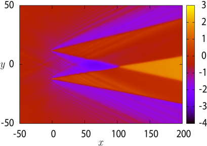
Figure 4: Left: Cross sections of the density distribution for different values of $x$ obtained from the numerical solution of the 2D NLS equation (1). The value of $x$ is indicated on each curve. We consider the flow past two different obstacles, one with radius $r=1.0$ at $(x_{10},y_{10})=(0,-12)$ and the other one with radius $r=0.6$ located at $(x_{20},y_{20})=(0,12)$. The collision of two different oblique dark solitons occurs at $x\approx 103$ and is still practically elastic. The solitons angles are $\theta_{1}=0.1$ and $\theta_{2}=0.13$ and the shifts of the solitons positions are $\Delta y_{1}\approx\Delta y_{2}\approx 0.5$. Right: Density plot of the corresponding phase. We can see a phase jump after the collision of the two solitons. .

References

- (1) B.B. Kadomtsev and V.I. Petviashvili, Sov. Phys. Doklady, 15, 539 (1970).
- (2) V.E. Zakharov, JETP Lett. 22, 172 (1975).
- (3) E.A. Kuznetsov and S.K. Turitsyn, Sov. Phys. JETP, 67, 1583 (1988). [Zh. Eksp. Teor. Fiz. 94, 119 (1988)].
- (4) G.A. El, A. Gammal, and A.M. Kamchatnov, Phys. Rev. Lett. 97, 180405 (2006).
- (5) A.M. Kamchatnov and L.P. Pitaevskii, Phys. Rev. Lett. 100, 160402 (2008).
- (6) A.M. Kamchatnov and S.V. Korneev, Phys. Lett. A 375, 2577 (2011).
- (7) E.G. Khamis, A. Gammal, G.A. El, Yu.G. Gladush, and A. M. Kamchatnov, Phys. Rev. A 78, 013829 (2008).
- (8) A. Amo et al., Science 332, 1167 (2011).
- (9) V.E. Zakharov, S.V. Manakov, S.P. Novikov, L.P. Pitaevskii, Theory of solitons, Moscow, Nauka, 1980.
- (10) G.A. El and A.M. Kamchatnov, Phys. Lett. A 350, 192 (2006); erratum: Phys. Lett. A 352, 554 (2006).
- (11) G. A. El, A. M. Kamchatnov, V. V. Khodorovskii, E. S. Annibale, and A. Gammal, Phys. Rev. E 80, 046317 (2009).
- (12) G.A. El, Yu.G. Gladush, and A.M. Kamchatnov, J. Phys. A: Math. Theor. 40, 611 (2007).
- (13) V.E. Zakharov and A.B. Shabat, Sov. Phys. JETP 37, 823 (1973) [Zh. Eksp. Teor. Fiz. 64, 1627 (1973)].
- (14) Yu.G. Gladush, G.A. El, A. Gammal, A.M. Kamchatnov, Phys. Rev. A 75, 033619 (2007).