On the persistence and global stability of mass-action systems

Abstract

This paper concerns the long-term behavior of population systems, and in particular of chemical reaction systems, modeled by deterministic mass-action kinetics. We approach two important open problems in the field of Chemical Reaction Network Theory, the Persistence Conjecture and the Global Attractor Conjecture. We study the persistence of a large class of networks called lower-endotactic and in particular, we show that in weakly reversible mass-action systems with two-dimensional stoichiometric subspace all bounded trajectories are persistent. Moreover, we use these ideas to show that the Global Attractor Conjecture is true for systems with three-dimensional stoichiometric subspace.

1 Introduction

Mass-action systems are a large class of nonlinear differential equations, widely used in the modeling of interaction networks in chemistry, biology and engineering. Due to the high complexity of dynamical systems arising from nonlinear interactions, it is very difficult, if not impossible, to create general mathematical criteria about qualitative properties of such systems, like existence of positive equilibria, stability properties of equilibria or persistence (non-extinction) of variables. However, a fertile theory that answers this type of questions for mass-action systems has been developed over the last 40 years in the context of chemical reaction systems. Generally termed “Chemical Reaction Network Theory” [11, 12, 13, 14, 17, 18, 19, 20] this field of research originated with the seminal work of Fritz Horn, Roy Jackson and Martin Feinberg [11, 18, 20] and describes the surprisingly stable dynamic behavior of large classes of mass-action systems, independently of the values of the parameters present in the system. This fact is very relevant, since the exact values of the system parameters are typically unknown in practical applications. Although the results in this paper will be applicable to general population systems driven by mass-action kinetics, they will be developed within the frame of Chemical Reaction Network Theory.

A large part of this paper is devoted to persistence properties of mass-action systems. A dynamical system on $\mathbb{R}^{n}_{\geq 0}$ is called persistent if forward trajectories that start in the interior of the positive orthant do not approach the boundary of $\mathbb{R}^{n}_{\geq 0}$ (see section 2.6 for a rigorous definition). Note that, throughout this paper, trajectory will always mean bounded trajectory. For systems with bounded trajectories, this is equivalent to saying that no trajectories with positive initial condition have $\omega$-limit points on the boundary of $\mathbb{R}^{n}_{\geq 0}.$ Persistence answers important questions regarding dynamic properties of biochemical systems, ecosystems, or infectious diseases, e.g. will each chemical species be available at all future times; or will a species become extinct in an ecosystem; or will an infection die off. One of the major open questions of Chemical Reaction Network Theory is the following:

Persistence Conjecture [10]. Any weakly reversible mass-action system is persistent.

A weakly reversible mass-action system is one for which its directed reaction graph has strongly connected components (Definition 3). A version of this conjecture was first mentioned by Feinberg in [13, Remark 6.1.E]; that version only requires that no trajectory with positive initial condition converges to a boundary point. A stronger version of the Persistence Conjecture (called the Extended Persistence Conjecture) was formulated by Craciun, Nazarov and Pantea in [10] and it was shown to be true for two-species systems. Moreover, in that case, weakly reversible mass-action systems are not only persistent, but also permanent (all trajectories originating in the interior of $\mathbb{R}^{n}_{\geq 0}$ eventually enter a fixed compact subset of the interior of $\mathbb{R}^{n}_{\geq 0}$).

In recent approaches to the Persistence Conjecture, the behavior of weakly reversible mass-action systems near the faces of their stoichiometric compatibility classes (minimal linear invariant subsets) was considered. It is known that $\omega$-limit points may only lie on faces of the stoichiometric compatibility class that are associated with a semilocking set [1] (see also [13, Remark 6.1.E]), or siphon in the Petri net literature [5, 27]. Anderson [1] and Craciun, Dickenstein, Shiu and Sturmfels [9] showed that vertices of the stoichiometric compatibility class cannot be $\omega$-limit points. Moreover, Anderson and Shiu [4] proved that for a weakly reversible mass-action system, the trajectories are, in some sense, repelled away from codimension-one faces of the stoichiometric compatibility class.

In this paper we prove the following version of the Persistence Conjecture for systems with two-dimensional stoichiometric compatibility classes (Theorem 5.1):

Theorem 5.1. Any $\kappa$-variable mass-action system with bounded trajectories, two-dimensional stoichiometric compatibility classes and lower-endotactic stoichiometric subnetworks is persistent.

Here a stoichiometric subnetwork is a union of connected components of the reaction graph (see Definition 8) and the requirement of lower-endotactic (Definition 17) stoichiometric subnetworks is less restrictive than that of weak reversibility. We suggest that the hypothesis of “lower-endotactic” arises naturally in the context of persistence of mass-action systems. Moreover, $\kappa$-variable mass-action is a generalization of mass-action where each reaction rate parameter is allowed to vary within a compact subset of $(0,\infty)$ (see Definition 6). Therefore this theorem implies the following:

Corollary. Any weakly reversible mass-action system with two-dimensional stoichiometric compatibility classes and bounded trajectories is persistent.

Note that our proof of Theorem 5.1. above (and of its corollary) requires the hypothesis of bounded trajectories. However, it has been conjectured that all trajectories of weakly reversible mass-action systems are bounded [3], and this conjecture has recently been proved for networks whose reaction graph has a single connected component [3]. Also, a stronger statement is known to be true for two-species networks: any endotactic, $\kappa$-variable mass-action system with two species has bounded trajectories [10].

The Persistence Conjecture is strongly related to another conjecture which is often considered the most important open problem in the field of Chemical Reaction Network Theory [2, 4, 9, 10], namely the Global Attractor Conjecture. This conjecture was first formulated by Horn [19] and concerns the long-term behavior of complex-balanced systems, i.e., systems that admit a positive complex-balanced equilibrium (see Definition 10). Horn and Jackson showed that if a mass-action system is complex-balanced then there exists a unique positive equilibrium in each stoichiometric compatibility class and this equilibrium is complex-balanced [20]. Moreover, each such equilibrium is locally asymptotically stable in its stoichiometric compatibility class due to the existence of a strict Lyapunov function [20]. In two subsequent papers [11, 18] Feinberg and Horn showed that weakly reversible mass-action systems which are also deficiency zero (Definition 11) are complex-balanced. This fact is remarkable since it reveals a wide class of reaction systems that are complex-balanced only because of their structure and regardless of parameter values. For a self-contained treatment of Chemical Reaction Network Theory, including the results mentioned above, the reader is referred to [12].

The Lyapunov function of Horn and Jackson does not guarantee global stability for a positive equilibrium relative to the interior of its compatibility class. This fact is the object of the Global Attractor Conjecture:

Global Attractor Conjecture. In a complex-balanced mass-action system, the unique positive equilibrium of a stoichiometric compatibility class is a global attractor of the interior of that class.

It is known [12] that complex-balanced systems are necessarily weakly reversible. On the other hand, trajectories of complex-balanced systems converge to the set of equilibria [1, 24, 26], so it follows that the Persistence Conjecture implies the Global Attractor Conjecture.

A series of partial results towards a proof of the Global Attractor Conjecture have been obtained in recent years. It is known that the conjecture is true for systems with two-dimensional stoichiometric compatibility classes ([4]; see also the recent work of Siegel and Johnston [25]), and for three-species systems [10]. Recently, Anderson proved that the conjecture holds if the reaction graph has a single connected component [2].

In this paper we prove the Global Attractor Conjecture for systems with three-dimensional stoichiometric compatibility classes (Theorem 6.3):

Theorem 6.3. Consider a complex-balanced weakly reversible mass-action system having stoichiometric compatibility classes of dimension three. Then, for any positive initial condition $c_{0},$ the solution $c(t)$ converges to the unique positive equilibrium which is stoichiometrically compatible with $c_{0}.$

Aside from being significant in the field of polynomial dynamical systems and relevant in important biological models [15, 16, 24, 26], Chemical Reaction Network Theory, and in particular the two conjectures discussed above, have ramifications in other well-established areas of mathematics. For example, [9] stresses the connection with toric geometry and computational algebra; in that work complex-balanced systems are called toric dynamical systems to emphasize their intrinsic algebraic structure. Also, [23] studies the rich algebraic structure of biochemical reaction systems with toric steady states. Furthermore, the unique positive equilibrium in a stoichiometric compatibility class of a complex-balanced system is sometimes called the Birch point in relation to Birch’s Theorem from algebraic statistics [9, 21].

This paper is organized as follows. After a preliminary section of terminology and notation, we introduce the lower-endotactic networks in section 3 and follow with a discussion of our main technical tool, the 2D-reduced mass-action system in section 4. The main persistence result of the paper is contained in section 5 (Theorem 5.1) and our result on the Global Attractor Conjecture (Theorem 6.3) is proved in section 6. A critical part in the proof of the latter theorem resides in the result of Theorem 6.2, which analyzes the behavior of weakly reversible mass-action systems near codimension-two faces of stoichiometric compatibility classes.

2 Preliminaries

A chemical reaction network is usually given by a finite list of reactions that involve a finite set of chemical species. An example with four species $A,B,C$ and $D$ and five reactions is given in (1).

$$B+D\displaystyle\mathop{\rightleftharpoons}A+C\displaystyle\mathop{\to}A+B\displaystyle\mathop{\to}C+D\qquad 2A\displaystyle\mathop{\to}A+D\displaystyle\mathop{\leftarrow}2D$$ (1)

The interpretation of the reaction $A+B\to C+D$, for instance, is that one molecule of species $A$ combines with one molecule of species $B$ to produce one molecule of each of the species $C$ and $D$. The objects on both sides of a reaction are formal linear combinations of species and are called complexes. According to the direction of the reaction arrow, a complex is either source or target. This way, the reaction $A+B\to C+D$ in (1) has $A+B$ as source complex and $C+D$ as target complex. The concentrations $c_{A},c_{B},c_{C}$ and $c_{D}$ vary with time by means of a set of ordinary differential equations, which we will explain shortly. In this preliminary section of the paper we review the standard concepts of Chemical Reaction Network Theory (see [12]) and introduce some new terminology that will be useful further on. In what follows, the set of nonnegative, respectively strictly positive real numbers are denoted by $\mathbb{R}_{\geq 0}$ and $\mathbb{R}_{>0}$ . For an integer $n\geq 1$ we call $\mathbb{R}_{>0}^{n}$ the positive orthant. The boundary of a set $K\subset\mathbb{R}^{n}$ will be denoted by $\partial K$ and the convex hull of $K$ will be denoted by $\mathrm{conv}(K).$ Also, we will denote the transpose of a matrix $A$ by $A^{t}.$

2.1 Reaction networks

If $I$ is a finite set then we denote by ${\mathbb{Z}}_{\geq 0}^{I}$ and ${\mathbb{R}}_{\geq 0}^{I}$ the set of all formal sums $\alpha=\displaystyle\sum_{i\in I}\alpha_{i}i$ where $\alpha_{i}$ are nonnegative integers, respectively nonnegative reals.

Definition 1.

A chemical reaction network is a triple $(\mathcal{S},\mathcal{C},\mathcal{R})$, where $\mathcal{S}$ is the set of species, $\mathcal{C}\subseteq\mathbb{Z}_{\geq 0}^{\mathcal{S}}$ is the set of complexes, and $\mathcal{R}$ is a relation on $\mathcal{C}$, denoted $P\to P^{\prime}$, representing the set of reactions of the network. The reaction set $\mathcal{R}$ cannot contain elements of the form $P\to P$ and each complex in $\mathcal{C}$ is required to appear in at least one reaction.

For simplicity, we will often denote a reaction network by a single letter, for instance $\mathcal{N}=(\mathcal{S},\mathcal{C},\mathcal{R}).$ For technical reasons we have chosen to neglect a third requirement that is usually included in the definition of a reaction network (see [12]): each species appears in at least one complex. This condition is not essential in the setting of this paper.

In (1) the set of species is $\mathcal{S}=\{A,B,C,D\}$, and the set of complexes is $\mathcal{C}=\{B+D,A+C,A+B,C+D,2A,A+D,2D\}.$

Once we fix an order among the species, any complex may be viewed as a column vector of dimension equal to the number of elements of $\mathcal{S}.$ For example, the complexes $A+B$ and $2D$ in (1) may be represented by the vectors $(1\ 1\ 0\ 0)^{t},$ and $(0\ 0\ 0\ 2)^{t}.$ With this identification in place, we may now define the reaction vector of a reaction $P\to P^{\prime}\in\mathcal{R}$ to be $P^{\prime}-P.$

Definition 2.

The stoichiometric subspace of the reaction network $\mathcal{N}=(\mathcal{S},\mathcal{C},\mathcal{R})$ is $S=\mathrm{span}\{P^{\prime}-P\mid P\to P^{\prime}\in\mathcal{R}\}.$

Example 1.

The stoichiometric subspace of the reaction network (1) is the column space of the stoichiometric matrix

$$A=\left(\begin{tabular}[]{rrrrrr}1&-1&0&-1&-1&1\\ -1&1&1&-1&0&0\\ 1&-1&-1&1&0&0\\ -1&1&0&1&1&-1\\ \end{tabular}\right).$$

It is easy to see that $S=\{(a,\ b,\ -b,\ -a)^{t}|(a,b)\in\mathbb{R}^{2}\}.$

Any reaction network $\mathcal{N}$ can be viewed as a directed graph whose vertices are the complexes of $\mathcal{N}$ and whose edges correspond to reactions of $\mathcal{N}$. Each connected component of this graph is called a linkage class of $\mathcal{N}.$

Definition 3.

A reaction network $\mathcal{N}$ is called weakly reversible if its associated directed graph has strongly connected components.

In other words, $\mathcal{N}$ is weakly reversible if whenever there exists a directed arrow pathway (consisting of one or more reaction arrows) from one complex to another, there also exists a directed arrow pathway from the second complex back to the first.

2.2 Reaction systems

Throughout this paper we let $n$ denote the number of species of a reaction network $\mathcal{N}=(\mathcal{S},\mathcal{C},\mathcal{R}),$ we fix an order among the species, and we denote $\mathcal{S}=\{X_{1},\ldots,X_{n}\}.$ We also let $c(t)\in\mathbb{R}^{\mathcal{S}}\cong\mathbb{R}^{n}$ denote the (column) vector of species concentrations at time $t\geq 0$. From here on, “vector” or “point of $\mathbb{R}^{n}$” will always mean “column vector”, even if, for simplicity, the notation ^t may not always be used. The concentration vector $c(t)$ is governed by a set of ordinary differential equations that involve a reaction rate function for each reaction in ${\mathcal{R}}.$

Definition 4.

A (non-autonomous) reaction system is a quadruple $({\mathcal{S}},{\mathcal{C}},{\mathcal{R}},K)$ where $\mathcal{N}=({\mathcal{S}},{\mathcal{C}},{\mathcal{R}})$ is a reaction network with $n$ species and $K:\mathbb{R}_{\geq 0}\times\mathbb{R}_{\geq 0}^{n}\to\mathbb{R}_{>0}^{\mathcal{R}}$ is a piecewise differentiable function called the kinetics of the system. The component $K_{P\to P^{\prime}}$ of $K$ is called the rate function of reaction $P\to P^{\prime}.$ Letting $P=(m_{1},\ldots,m_{n})$ and ${\bf x}=(x_{1},\ldots,x_{n}),$ $K_{P\to P^{\prime}}$ is assumed to satisfy, for any $t\geq 0,$ the following: if $x_{i}=0$ and $m_{i}\neq 0$ then $K_{P\to P^{\prime}}(t,{\bf x})=0.$ The dynamics of the system is given by the following system of differential equations for the concentration vector $c(t)$:

$$\dot{c}(t)=\sum_{P\to P^{\prime}}K_{P\to P^{\prime}}(t,c(t))(P^{\prime}-P).$$ (2)

Note that we will often use the short notation $(\mathcal{N},K)$ for a reaction system.

The regularity condition on $K$ may be replaced by any other condition that guarantees uniqueness of solutions for (2). Sometimes, additional properties are required of $K$ [4, 6, 7]. For example, it is commonly assumed that if the $i$th species is not a reactant in $P\to P^{\prime}$ (i.e. $m_{i}=0$) then $K_{P\to P^{\prime}}$ does not depend on $x_{i}.$ Another widespread assumption is that $K$ is increasing with respect to reactant concentrations, i.e. $\frac{\partial}{\partial x_{i}}K_{P\to P^{\prime}}\geq 0$ if $m_{i}\neq 0.$ These conditions are automatically satisfied for the kinetics treated in this paper.

If $c_{0}\in\mathbb{R}^{n}_{\geq 0}$ we let

$$T(c_{0})=\{c(t)\mid t\geq 0,c(0)=c_{0}\}$$

denote the trajectory of $(\mathcal{N},K)$ with initial condition $c_{0}.$ If $K(t,{\bf x})=K({\bf x})$ does not depend explicitly on time, we say that $c_{*}\in\mathbb{R}^{n}_{\geq 0}$ is an equilibrium of the reaction system $(\mathcal{N},K)$ if it is an equilibrium of the corresponding differential equations (2).

Note that the condition on $K_{P\to P^{\prime}}$ imposed in Definition 4 makes the nonnegative orthant $\mathbb{R}^{n}_{\geq 0}$ forward invariant for (2). Under mild additional assumptions on $K,$ the positive orthant $\mathbb{R}^{n}_{>0}$ is also forward-invariant for (2) (see [26]). For example, this will be the case for $\kappa$-variable mass-action kinetics, the main type of kinetics considered in this paper (Definition 6).

Integrating (2) yields

$$c(t)=c(0)+\sum_{P\to P^{\prime}}\left(\int_{0}^{t}K_{P\to P^{\prime}}(s,c(s))ds\right)(P^{\prime}-P)$$

and it follows that $c(t)$ is contained in the affine subspace $c(0)+S$ for all $t\geq 0.$ Combining this with the preceding observation we see that $(c(0)+S)\cap\mathbb{R}_{\geq 0}^{n}$ is forward invariant for (2).

Definition 5.

Let $c_{0}\in\mathbb{R}^{n}.$ The polyhedron $(c_{0}+S)\cap\mathbb{R}_{\geq 0}^{n}$ is called the stoichiometric compatibility class of $c_{0}.$

Note that, throughout this paper, “polyhedron” will always mean “convex polyhedron”, i.e., an intersection of finitely many half-spaces. To prepare for the next definition we introduce the following notation: given two vectors $u,v\in\mathbb{R}^{n}_{\geq 0},$ we denote $u^{v}=\displaystyle\prod_{i=1}^{n}u_{i}^{v_{i}}$, with the convention $0^{0}=1$.

Definition 6 ([10]).

A $\kappa$-variable mass-action system is a reaction system $(\mathcal{N},K)$ where $\mathcal{N}=(\mathcal{S},\mathcal{C},\mathcal{R})$ and the rate function of $P\to P^{\prime}\in\mathcal{R}$ is given by

$$K_{P\to P^{\prime}}(t,{\bf x})=\kappa_{P\to P^{\prime}}(t){\bf x}^{P}.$$ (3)

Here $\kappa:\mathbb{R}_{\geq 0}\to(\eta,1/\eta)^{\mathcal{R}}$ for some $\eta<1$ is a piecewise differentiable function called the rate-constant function.

To emphasize the rate-constant function, we denote a $\kappa$-variable mass-action system by $(\mathcal{S},\mathcal{C},\mathcal{R},\kappa),$ or by $(\mathcal{N},\kappa).$ Note that if the rate-constant function is fixed in time, $\kappa$-variable mass-action becomes the usual mass-action. A few biological examples of $\kappa$-variable mass-action models that are not mass-action are presented in [10].

Therefore, a $\kappa$-variable mass-action system gives rise to the following non-autonomous, and usually nonlinear, system of coupled differential equations:

$$\dot{c}(t)=\sum_{P\to P^{\prime}}\kappa_{P\to P^{\prime}}(t)c(t)^{P}(P^{\prime}-P).$$ (4)

Example 2.

We endow the reaction network (1) with $\kappa$-variable mass-action kinetics of rate-constant function specified on the reaction arrows in (5).

$$B+D\displaystyle\mathop{\rightleftharpoons}^{\kappa_{1}(t)}_{\kappa_{2}(t)}A+C\displaystyle\mathop{\to}^{\kappa_{3}(t)}A+B\displaystyle\mathop{\to}^{\kappa_{4}(t)}C+D\qquad 2A\displaystyle\mathop{\to}^{\kappa_{5}(t)}A+D\displaystyle\mathop{\leftarrow}^{\kappa_{6}(t)}2D$$ (5)

We have $c(t)=(c_{A}(t),\ c_{B}(t),\ c_{C}(t),\ c_{D}(t))$ and note that, for example, $c(t)^{A+B}=c(t)^{(1\ 1\ 0\ 0)}=c_{A}(t)c_{B}(t).$ From (4) we have

$$\dot{c}=\kappa_{1}(t)c_{B}c_{D}A_{1}+\kappa_{2}(t)c_{A}c_{C}A_{2}+\kappa_{3}(t)c_{A}c_{C}A_{3}+\kappa_{4}(t)c_{A}c_{B}A_{4}+\kappa_{5}(t)c_{A}^{2}A_{5}+\kappa_{6}(t)c_{D}^{2}A_{6}$$

for all $t\geq 0,$ where $A_{i}$ is column $i$ of the stoichiometric matrix $A$ given in (1), i.e., the reaction vector of reaction $i.$ Therefore the differential equations corresponding to (5) are

$$\dot{c}_{A} = \kappa_{1}(t)c_{B}c_{D}-\kappa_{2}(t)c_{A}c_{C}-\kappa_{4}(t)c_{A}c_{B}-\kappa_{5}(t)c_{A}^{2}+\kappa_{6}(t)c_{D}^{2}$$ (6)

$$\dot{c}_{B} = -\kappa_{1}(t)c_{B}c_{D}+\kappa_{2}(t)c_{A}c_{C}+\kappa_{3}(t)c_{A}c_{C}-\kappa_{4}(t)c_{A}c_{B}$$

$$\dot{c}_{C} = \kappa_{1}(t)c_{B}c_{D}-\kappa_{2}(t)c_{A}c_{C}-\kappa_{3}(t)c_{A}c_{C}+\kappa_{4}(t)c_{A}c_{B}$$

$$\dot{c}_{D} = -\kappa_{1}(t)c_{B}c_{D}+\kappa_{2}(t)c_{A}c_{C}+\kappa_{4}(t)c_{A}c_{B}+\kappa_{5}(t)c_{A}^{2}-\kappa_{6}(t)c_{D}^{2},$$

2.3 Sums of reaction systems

A reaction network $(\mathcal{S},\mathcal{C},\mathcal{R})$ is called a subnetwork of $(\mathcal{S},^{\prime}\mathcal{C}^{\prime},\mathcal{R}^{\prime})$ if $\mathcal{S}\subseteq\mathcal{S}^{\prime}$, $\mathcal{C}\subseteq\mathcal{C}^{\prime}$ and $\mathcal{R}\subseteq\mathcal{R}^{\prime}.$ If $\mathcal{R}^{\prime}$ has an associated kinetics $K$ then restricting $K$ to reactions of $\mathcal{R}$ defines a kinetics for $\mathcal{R}.$ On the other hand, if $\mathcal{N}_{s}=(\mathcal{S}_{s},\mathcal{C}_{s},\mathcal{R}_{s})$, $s\in\{1,\ldots,p\}$ are reaction networks, their union, denoted by $\bigcup_{s=1}^{p}(\mathcal{S}_{s},\mathcal{C}_{s},\mathcal{R}_{s})$ or simply by $\bigcup_{s=1}^{p}\mathcal{N}_{s}$, and defined as the triple $(\bigcup_{s=1}^{p}\mathcal{S}_{s},\bigcup_{s=1}^{p}\mathcal{C}_{s},\bigcup_{s=1}^{p}\mathcal{R}_{s})$ is also a reaction network. If each $\mathcal{N}_{s}$ has an associated kinetics $K_{s},$ we can define a kinetics for $\bigcup_{s=1}^{p}\mathcal{N}_{s}$ by simply adding all $K_{s}.$

Definition 7.

The sum of the reaction systems $(\mathcal{S}_{s},\mathcal{C}_{s},\mathcal{R}_{s},K_{s})$ is the reaction system $(\mathcal{S},\mathcal{C},\mathcal{R},K)$ where $(\mathcal{S},\mathcal{C},\mathcal{R})=\bigcup_{s=1}^{p}(\mathcal{S}_{s},\mathcal{C}_{s},\mathcal{R}_{s})$ and

$$K_{P\to P^{\prime}}(t,{\bf x})=\sum_{\{s:P\to P^{\prime}\in\mathcal{R}_{s}\}}K_{s,P\to P^{\prime}}(t,\bf x)$$

for and all $(t,{\bf x})\in\mathbb{R}_{\geq 0}\times\mathbb{R}^{n}_{\geq 0}.$ We will denote this $(\mathcal{S},\mathcal{C},\mathcal{R},K)$ by $\bigcup_{s=1}^{p}(\mathcal{S}_{s},\mathcal{C}_{s},\mathcal{R}_{s},K_{s})$ or simply by $\bigcup_{s=1}^{p}(\mathcal{N}_{s},K_{s}),$ where $\mathcal{N}_{s}=(\mathcal{S}_{s},\mathcal{C}_{s},\mathcal{R}_{s}).$

For example, any reaction system is the sum of the reaction systems corresponding to its linkage classes. Similarly, any reaction system is the sum of the reaction systems corresponding to its stoichiometric subnetworks, which we define next.

Definition 8.

A reaction network $(\mathcal{S},\mathcal{C},\mathcal{R})$ with stoichiometric subspace $S$ can be written uniquely as a union of subnetworks

$$(\mathcal{S},\mathcal{C},\mathcal{R})=\bigcup_{s=1}^{p}(\mathcal{S}_{s},\mathcal{C}_{s},\mathcal{R}_{s})$$

where $\{{\mathcal{C}}_{s}\}_{s\in\{1,\ldots,p\}}$ is a partition of $\cal C$ such that two complexes in $\cal C$ are in the same block of the partition if and only if their difference is in $S$. We call each $(\mathcal{S}_{s},\mathcal{C}_{s},\mathcal{R}_{s})$ a stoichiometric subnetwork of $(\mathcal{S},\mathcal{C},\mathcal{R})$.

Fig. 1: Stoichiometric subnetworks for Example 3.

Example 3.

The diagram in Figure 1 represents the reaction network

$$C\to B\to A,\quad 2B\rightleftharpoons A+B,\quad B+C\to 2A\to 2C.$$

This reaction network has three linkage classes, and two stoichiometric subnetworks

$$\{C\to B\to A\}\text{ and }\{2B\rightleftharpoons A+B,\quad B+C\to 2A\to 2C\}.$$

Note that there exist vectors $a_{1},\ldots,a_{p}\in\mathbb{R}^{n}$ such that for all $s\in\{1,\ldots,p\},$ we have $\mathcal{C}_{s}\subset a_{s}+S$ and the affine subspaces $a_{s}+S,$ $s\in\{1,\ldots,p\}$ are pairwise disjoint. Also note that each stoichiometric subnetwork is a union of linkage classes.

Example 4.

The reaction network (1) has two linkage classes which belong to two different stoichiometric subnetworks since $(A+B)-2A=(-1,\ 1,\ 0,\ 0)\notin S$ (recall $S$ from Example 1). Therefore the reaction network has exactly two stoichiometric subnetworks which coincide with its linkage classes.

2.4 Projected reaction systems

For $W\subset\{1,\ldots,n\}$ we define

$$\pi_{W}:\mathbb{R}^{n}\to\mathbb{R}^{W}$$

to be the projection onto W, i.e. the orthogonal projection onto $\mathbb{R}^{W}.$

Definition 9 ([22]; see also [2]).

Let $\mathcal{N}=(\mathcal{S},\mathcal{C},\mathcal{R})$ be a reaction network with $\mathcal{S}=\{X_{1},\ldots,X_{n}\}$ and let $W\subset\{1,\ldots,n\}.$ Let $\mathcal{S}_{W}=\{X_{i}\mid i\in W\},$

$$\mathcal{R}_{W}=\{\pi_{W}(P)\to\pi_{W}(P^{\prime})\mid P\to P^{\prime}\in\mathcal{R},\text{ such that }\pi_{W}(P)\neq\pi_{W}(P^{\prime})\}$$

and $\mathcal{C}_{W}\subset\pi_{W}(\mathcal{C})$ be the set of complexes in $\mathcal{R}_{W}.$ The reaction network $(\mathcal{S}_{W},\mathcal{C}_{W},\mathcal{R}_{W}),$ is called $\mathcal{N}$ projected onto $W$ and denoted $\pi_{W}(\mathcal{N}).$

In other words, the projection of $(\mathcal{S},\mathcal{C},\mathcal{R})$ onto $W$ is obtained by deleting the species $X_{i}$, $i\in\complement W$ from all reactions in $\mathcal{R}$ and further removing the resulting reactions for which the source and the target complexes are the same. Here and from now on $\complement W$ denotes the complement of $W$ in $\{1,\ldots,n\}$.

If $(\mathcal{N},K)=(\mathcal{S},\mathcal{C},\mathcal{R},K)$ is a reaction system and $c(t)=(c_{1}(t),\ldots,c_{n}(t))$ is a solution of the corresponding system of differential equations (2) with initial condition $c_{0}\in\mathbb{R}^{n}_{\geq 0},$ then $\pi_{W}(c)(t)$ is a solution of the following system of differential equations:

$$\frac{d}{dt}\pi_{W}(c)=\sum_{Q\to Q^{\prime}\in\mathcal{R}_{W}}\Bigg{(}\sum_{\begin{subarray}{c}{\{P\to P^{\prime}\in\mathcal{R}:}\\ {\pi_{W}(P)=Q,\pi_{W}(P^{\prime})=Q^{\prime}\}}\end{subarray}}\overline{K}_{P\to P^{\prime}}(t,\pi_{W}(c))\Bigg{)}(Q^{\prime}-Q)$$ (7)

with initial condition $\pi_{W}(c_{0}).$ Equation (7) is obtained from (2) by $(i)$ keeping only the equations for $\dot{c}_{i}$ with $i\in W$; $(ii)$ writing $K_{P\to P^{\prime}}(t,c)=\overline{K}_{P\to P^{\prime}}(t,\pi_{W}(c))$ to illustrate that $c_{i},$ $i\in\complement W,$ are written either in terms of $c_{i},$ $i\in W,$ or as functions of $t;$ and $(iii)$ lumping together the rates of reactions $P\to P^{\prime}$ that project to the same reaction in $\mathcal{R}_{W}.$ The system of differential equations (7) defines a kinetics $K_{W}$ for $\pi_{W}(\mathcal{N}),$ where, for any reaction $Q\to Q^{\prime}\in{\cal R}_{W},$ $K_{W,Q\to Q^{\prime}}$ is given by the sum from the parentheses in (7). We call the resulting reaction system $(\pi_{W}(\mathcal{N}),K_{W})$ a projection of $\mathcal{N}$ onto $W$. Note that $\overline{K}$ is not unique. Which variables $c_{i},$ $i\in\complement W$ are written in terms of $t$ and which are written in terms of $c_{i},$ $i\in W$ is a matter of context. For instance, Example 5 below describes two different functions $\overline{K}$ associated with system (5) projected onto $\{1,2\}.$

A natural way of defining $\overline{K}$ for $\kappa$-variable mass-action systems is to include $c_{i},$ $i\in\complement W$ in the rate-constant function: $\overline{K}(t,c)=\overline{\kappa}(t)\pi_{W}(c)^{\pi_{W}(P)},$ where $\overline{\kappa}(t)=\kappa(t)\pi_{\complement W}(c(t))^{\pi_{\complement W}(P)}.$ The differential equations (7) in this case are

$$\frac{d}{dt}\pi_{W}(c)=\sum_{Q\to Q^{\prime}\in\mathcal{R}_{W}}\Bigg{(}\sum_{\begin{subarray}{c}{\{P\to P^{\prime}\in\mathcal{R}:}\\ {\pi_{W}(P)=Q,\pi_{W}(P^{\prime})=Q^{\prime}\}}\end{subarray}}\kappa_{P\to P^{\prime}}(t)\pi_{\complement W}(c)^{\pi_{\complement W}(P)}\Bigg{)}\pi_{W}(c)^{Q}(Q^{\prime}-Q).$$ (8)

Note that this projection has the form of $\kappa$-variable mass-action, with rate-constant function for the reaction $Q\to Q^{\prime}\in\mathcal{R}_{W}$ given by the second sum in (8). However, this rate-constant is not necessarily bounded in a compact interval of $(0,\infty).$

Example 5.

Following (8), the projection of reaction system (5) onto $W=\{1,2\}$ i.e., onto species $A$ and $B,$ can be written in the $\kappa$-variable mass-action form (without necessarily being $\kappa$-variable mass-action):

$$B\mathop{\rightleftharpoons}^{\overline{\kappa}_{1}(t)}_{\overline{\kappa}_{2}(t)}A\mathop{\to}^{\overline{\kappa}_{3}(t)}A+B\mathop{\to}^{\kappa_{4}(t)}0\qquad 2A\mathop{\to}^{\kappa_{5}(t)}A\mathop{\leftarrow}^{\overline{\kappa}_{6}(t)}0$$

with differential equations

$$\dot{c}_{A} = \overline{\kappa}_{1}(t)c_{B}-\overline{\kappa}_{2}(t)c_{A}-\kappa_{4}(t)c_{A}c_{B}-\kappa_{5}(t)c_{A}^{2}+\overline{\kappa}_{6}(t)$$

$$\dot{c}_{B} = -\overline{\kappa}_{1}(t)c_{B}+\overline{\kappa}_{2}(t)c_{A}+\overline{\kappa}_{3}(t)c_{A}-\kappa_{4}(t)c_{A}c_{B}$$

where (recall equation (6)) $\overline{\kappa}_{1}(t)=\kappa_{1}(t)c_{D}(t),$ $\overline{\kappa}_{2}(t)=\kappa_{2}(t)c_{C}(t),$ $\overline{\kappa}_{3}(t)=\kappa_{3}(t)c_{C}(t),$ and $\overline{\kappa}_{6}(t)=\kappa_{6}(t)c_{D}(t)^{2}.$

On the other hand, let $T=\{c(t)\mid t\geq 0\}$ be a trajectory of (5) with initial condition $(\alpha,\ \beta,\ \gamma,\ \eta)\in\mathbb{R}_{>0}^{4}.$ Then $c_{A}+c_{D}=\alpha+\eta,$ $c_{B}+c_{C}=\beta+\gamma$ and therefore $\pi_{\{1,2\}}(T)$ is a trajectory of the following projection of (5):

$$B\mathop{\rightleftharpoons}^{\overline{K}_{1}}_{\overline{K}_{2}}A\mathop{\to}^{\overline{K}_{3}}A+B\mathop{\to}^{\overline{K}_{4}}0\qquad 2A\mathop{\to}^{\overline{K}_{5}}A\mathop{\leftarrow}^{\overline{K}_{6}}0,$$

where, denoting $\pi_{\{1,2\}}(c)=(x,y),$ the rate function $\overline{K}(t,(x,y))$ is given by $\overline{K}_{1}(t,(x,y))=\kappa_{1}(t)y(\alpha+\eta-x),$ $\overline{K}_{2}(t,(x,y))=\kappa_{2}(t)x(\beta+\gamma-y),$ $\overline{K}_{3}(t,(x,y))=\kappa_{3}(t)x(\beta+\gamma-y),$ $\overline{K}_{4}(t,(x,y))=\kappa_{4}(t)xy,$ $\overline{K}_{5}(t,(x,y))=\kappa_{5}(t)x^{2}$ and $\overline{K}_{6}(t,(x,y))=\kappa_{6}(t)(\alpha+\eta-x)^{2}.$

Remark 2.1.

Let $W\subset\{1,\ldots,n\}$ and $P,P^{\prime}\in\mathcal{C}.$ If $\pi_{W}(P)\neq\pi_{W}(P^{\prime}),$ then any directed path in $\mathcal{R}$ from $P$ to $P^{\prime}$ projects onto a directed path from $\pi_{W}(P)$ to $\pi_{W}(P^{\prime})$ in $\mathcal{R}_{W}$. If, on the other hand, $\pi_{W}(P)=\pi_{W}(P^{\prime}),$ then a directed path from $P$ to $P^{\prime}$ either projects onto a cycle in ${\cal R}_{W}$ or is eliminated by the projection.

Therefore projection preserves weak reversibility: if $\mathcal{N}$ is weakly reversible, then so is $\pi(\mathcal{N}).$ This result appears in [22] and is also the object of Lemma 3.4. in [2].

2.5 Complex-balanced systems and deficiency of a network

Complex-balanced systems are defined in the context of mass-action kinetics, i.e., the rate-constants are fixed positive numbers.

Definition 10.

An equilibrium $c_{*}\in\mathbb{R}_{\geq 0}^{n}$ of a mass-action system $(\mathcal{R},\mathcal{S},\mathcal{C},\kappa)$ is called complex-balanced equilibrium if, at $c_{*}$, for any complex $P_{0}\in\cal C,$ the flow into $P_{0}$ is equal to the flow out of $P_{0}.$ More precisely, for each $P_{0}\in{\mathcal{C}}$ we have

$$\sum_{P\to P_{0}}\kappa_{P\to P_{0}}{c_{*}}^{P}=\sum_{P_{0}\to P}\kappa_{P_{0}\to P}{c_{*}}^{P_{0}}.$$

A complex-balanced system is a mass-action system that admits a strictly positive complex-balanced equilibrium.

Definition 11.

Let $(\mathcal{S},\mathcal{C},\mathcal{R})$ be a reaction network with $m$ complexes, $l$ linkage classes and whose stoichiometric subspace has dimension $s.$ The deficiency of the reaction network $\mathcal{R}$ is $m-l-s.$

The deficiency of a reaction network is always non-negative [12]. It has been shown that weakly reversible systems whose deficiency is equal to zero are complex-balanced [12]. This remarkable fact reveals a large class of mass-action systems which are complex-balanced regardless of the choice of their rate constants.

2.6 Persistence and the sub-tangentiality condition

Definition 12.

A trajectory $T(c_{0})=\{(x_{1}(t),\ldots,x_{n}(t))\mid t\geq 0\}$ with positive initial condition $c_{0}\in\mathbb{R}_{>0}^{n}$ of an n-dimensional dynamical system is called persistent if

$$\liminf_{t\to\infty}x_{i}(t)>0\ for\ all\ i\in\{1,\ldots,n\}.$$

Some authors call a trajectory that satisfies the condition in Definition 12 strongly persistent [29]. In their work, persistence requires only that $\limsup_{t\to\infty}x_{i}(t)>0$ for all $i\in\{1,\ldots,n\}.$ We say that a dynamical system (or a reaction system) is persistent if all its trajectories with strictly positive initial condition are persistent.

Definition 13.

Let $T(c_{0})=\{{\bf x}(t)\mid t\geq 0\}$ denote a forward trajectory of a dynamical system with initial condition $c_{0}\in\mathbb{R}_{>0}^{n}.$ The $\omega$-limit set of $T(c_{0})$ is

$$\textstyle\lim_{\omega}T(c_{0})=\{l\in\mathbb{R}^{n}\mid\lim_{n\to\infty}c(t_{n})=l\text{ for some sequence }t_{n}\to\infty\}.$$

The elements of $\lim_{\omega}T(c_{0})$ are called $\omega$-limit points of $T(c_{0})$.

Note that a bounded trajectory of a dynamical system with positive initial condition is persistent iff it has no $\omega$-limit points on $\partial\mathbb{R}_{\geq 0}^{n}.$

In this paper we will prove persistence of trajectories $T(c_{0})$ for reaction systems with special properties. Our approach will consist of showing that a certain convex polyhedron included in $\mathbb{R}^{n}_{>0}$ contains $T(c_{0}).$ To this end we will use the following version of a result of Nagumo [8]. Recall that for a closed, convex set $K\subset\mathbb{R}^{n}$ and for ${\bf x}\in K$ the normal cone of $K$ at $\bf x$ is defined as follows:

$$N_{K}({\bf x})=\{{\bf n}\in\mathbb{R}^{n}\mid{\bf n}\cdot({\bf y}-{\bf x})\leq 0\text{ for all }{\bf y}\in K\}.$$

Theorem 2.1 (Nagumo, [8]).

Let $K\subset\mathbb{R}^{n}$ be a closed, convex set. Assume that the system $\dot{\bf x}(t)=f(t,{\bf x}(t))$ has unique solution for any initial value, and let $T(c_{0})=\{{\bf x}(t)\mid t\geq 0,\ x(0)=c_{0}\}$ be a forward trajectory of this system with $c_{0}\in K.$ If for any $t_{0}\geq 0$ such that $x(t_{0})\in\partial K$ we have the sub-tangentiality condition

$${\bf n}\cdot f(t_{0},x(t_{0}))\leq 0\text{ for all }{\bf n}\in N_{K}(x(t_{0}))$$

then $T(c_{0})\subset K.$

3 Lower-endotactic networks

Let $\mathcal{N}=(\mathcal{S},\mathcal{C},\mathcal{R})$ be a reaction network with species $X_{1},\ldots,X_{n}$ and let $S\subseteq\mathbb{R}^{n}$ denote its stoichiometric subspace. By a useful abuse of notation, we view the source complexes of $\mathcal{N}$ as lattice points in $\mathbb{Z}^{n}:$

$${\mathcal{SC}}({\mathcal{N}})=\{(m_{1},\ldots,m_{n})\in\mathbb{Z}_{\geq 0}^{n}\mid m_{1}X_{1}+\ldots+m_{n}X_{n}\in\mathcal{C}\text{ is a source complex}\}.$$

In this section we revisit the notion of lower-endotactic network, first introduced in [10] for the case of two-species networks, and we extend it to planar reaction networks, defined below. We let $\mathrm{aff}(\mathcal{N})$ denote the affine hull of $\mathcal{C}$, i.e. the minimal affine subspace of $\mathbb{R}^{n}$ that contains $\mathcal{C}.$

Definition 14.

The reaction network $\mathcal{N}$ is called planar if $\mathrm{dim(aff}(\mathcal{N}))\leq 2.$

Let $\mathrm{aff}_{+}(\mathcal{N})=\mathrm{aff}(\mathcal{N})\cap\mathbb{R}^{n}_{\geq 0}.$ The following definition is similar to the one in [10, section 4].

Definition 15.

Let $\mathcal{N}=(\mathcal{S},\mathcal{C},\mathcal{R})$ be a reaction network such that $\mathrm{aff}(\mathcal{N})$ has dimension two and let $\bf v$ be a vector in S.

(i) The $\bf v$-essential subnetwork $\mathcal{N}_{\bf v}=(\mathcal{S},\mathcal{C}_{\bf v},\mathcal{R}_{\bf v})$ of $(\mathcal{S},\mathcal{C},\mathcal{R})$ is defined by the reactions of $\mathcal{R}$ whose reaction vectors are not orthogonal to $\bf v$:

$$\mathcal{R}_{\bf v}=\{P\to P^{\prime}\in{\cal R}\mid(P^{\prime}-P)\cdot{\bf v}\neq 0\};$$

$\mathcal{C}_{\bf v}$ is defined as the set of complexes appearing in reactions of $\mathcal{R}_{\bf v}.$

(ii) The $\bf v$-essential support of $\mathcal{N}$ is the supporting line $L$ of $\mathrm{conv}(\mathcal{SC(N}_{\bf v}))$ that is orthogonal to $\bf v$ and such that the positive direction of $\bf v$ lies on the same side of $L$ as $\mathcal{SC(N}_{\bf v});$ (in other words, for any $P\in\mathrm{aff}(\mathcal{N}),$ the intersection of the half-line $\{P+t{\bf v}|,t\geq 0\}$ with the half-plane bounded by $L$ that contains $\mathcal{SC(N}_{\bf v})$ is unbounded.) The line $L$ is denoted by $esupp^{\bf v}(\mathcal{N}).$

Fig. 2: (a) Essential supports corresponding to ${\bf v}_{1}$ and ${\bf v}_{2};$ (b) Example of a set of inward vectors; (c) Illustration for the proof of Lemma 19.

Figure 2(a) illustrates the notion of $\bf v$-essential support for a planar reaction network with six complexes and four reactions. This reaction network has two source complexes and note that ${\cal N}_{{\bf v}_{1}}$ is equal to $\cal N,$ whereas ${\cal N}_{{\bf v}_{2}}$ is strictly smaller than $\cal N$ and contains only one source complex.

We denote by $esupp^{\bf v}(\mathcal{N})_{<0}$ the intersection of $\mathrm{aff}_{+}(\mathcal{N})$ with the open half-plane in $\mathrm{aff}(\mathcal{N})$ bounded by $esupp^{\bf v}(\mathcal{N})$ that does not contain the positive direction of $\bf v:$

$$esupp^{\bf v}(\mathcal{N})_{<0}=\{P\in\mathrm{aff}_{+}(\mathcal{N})\mid(P-Q)\cdot{\bf v}<0\text{ for all }Q\in esupp^{\bf v}(\mathcal{N})\}$$

and we define $esupp^{\bf v}(\mathcal{N})_{>0}$ similarly.

Definition 16.

Let $C\subset\mathbb{R}^{n}$ be a closed and convex set, and let $S$ be the linear subspace of $\mathbb{R}^{n}$ such that the affine hull of $C$ is a translation of $S$. Then

$$\mathrm{iv}(C)=-\bigcup_{{\bf x}\in\partial C}(N_{C}({\bf x})\cap S)$$

is called the set of inward vectors of $C.$ Here $\partial C$ denotes the relative boundary of $C.$

An example of a set of inward vectors for a two-dimensional set $C$ is depicted in Figure 2(b).

Remark 3.1.

(i) $\mathrm{iv}(C)$ is a convex cone and if $C$ is bounded then $\mathrm{iv}(C)=S.$

(ii) If $C$ is a half-line then $\mathrm{iv}(C)$ consists of all vectors parallel with $C$ pointing in the unbounded direction of $C.$ If $C$ is a bounded line segment, then $\mathrm{iv}(C)$ consists of all vectors parallel with $C.$

(iii) If $\mathrm{aff}(C)$ has dimension two, then the set of inward vectors $\mathrm{iv}(C)$ is two-dimensional and consists of the normal vectors ${\bf v}\in S$ of all supporting lines $L$ of $C$ such that the positive direction of $\bf v$ is on the same side of $L$ as $C$ (see Figure 2(b) for an example).

Definition 17.

Let $\mathcal{N}$ be a planar reaction network with stoichiometric subspace $S.$ Then $\mathcal{N}$ is called lower-endotactic if the set

$$\{P\to P^{\prime}\mid P\in esupp^{\bf v}(\mathcal{N})\text{ and }P^{\prime}\in esupp^{\bf v}(\mathcal{N})_{<0}\}$$ (9)

is empty for all nonzero vectors ${\bf v}\in\mathrm{iv}(\mathrm{aff}_{+}(\mathcal{N})).$

Definition 17(ii) is easily explained by the “parallel sweep test” [10]. A reaction network $\mathcal{N}=(\mathcal{S},\mathcal{C},\mathcal{R})$ is lower-endotactic if and only if it passes the following test for any nonzero inward vector $\bf v$ of $\mathrm{aff}_{+}(\mathcal{N})$: sweep the plane $\mathrm{aff}(\mathcal{N})$ with a line $L$ orthogonal to $\bf v$, coming from infinity and going in the direction of $\bf v$, and stop when $L$ encounters a source complex corresponding to a reaction which is not parallel to $L$. Now check that no reaction with source on $L$ points towards the swept region. If $\mathcal{R}_{\bf v}=\O$, then all reaction vectors of $\mathcal{R}$ are perpendicular to $\bf v$ and $L$ never stops in the parallel sweep test. In this case we still say that the network has passed the test for $\bf v$.

A reaction network is lower-endotactic if its reactions with sources that are “closest” to the boundary of $\mathrm{aff}_{+}(\mathcal{N})$ point “inside” $\mathrm{aff}_{+}(\mathcal{N})$. Note that this special property of lower-endotactic networks in the lattice space $\mathbb{Z}^{n}_{\geq 0}$ is analogous with the behavior of persistent trajectories in the phase space $\mathbb{R}^{n}_{\geq 0}:$ once a persistent trajectory gets “close enough” to the relative boundary of its stoichiometric compatibility class $S(c_{0})$, it is pushed back “inside”. In this sense, the requirement that a reaction network be lower-endotactic appears very naturally in the context of persistence of a corresponding reaction system.

Remark 3.2.

Following [10], a planar reaction network $\mathcal{N}$ is called endotactic if the parallel sweep test holds for all nonzero vectors ${\bf v}\in S$. An endotactic network is also lower-endotactic; the two notions coincide if $\mathrm{aff}_{+}(\mathcal{N})$ is bounded.

Remark 3.3.

The definition of endotactic networks has been extended in [10] for networks that are not necesarilly planar, using the parallel sweep test with hyperplanes instead of lines ([10, Remark 4.1]). Definition 17 is in fact a special case of the following more general definition of lower-endotactic networks:

Definition 18.

A reaction network (not necessarily planar) with $n$ species is called lower-endotactic if it passes the parallel sweep test for any inward vector of the non-negative orthant $\mathbb{R}_{\geq 0}^{n}.$

Whereas the definition above is easier to state, the more technical Definition 17 is better suited for planar networks in the context of this paper.

Remark 3.4.

A weakly reversible reaction network $\mathcal{N}$ is always endotactic, and in particular, lower-endotactic. Indeed, if $P\in esupp^{\bf v}(\mathcal{N})$ for some vector ${\bf v}\in S$ and $P\to P^{\prime}$ is a reaction of $\mathcal{N}$ then $P^{\prime}\in esupp^{\bf v}(\mathcal{N})_{\geq 0},$ for otherwise the fact that $P^{\prime}$ is also a source complex would contradict $P\in esupp^{\bf v}(\mathcal{N}).$

Remark 3.5.

If $\mathrm{aff}(\mathcal{N})$ is one-dimensional we let $\mathcal{P}$ be a two-dimensional affine subspace of $\mathbb{R}^{n}$ such that $\mathrm{aff}(\mathcal{N})\subset\mathcal{P}.$ The parallel sweep test for $\mathcal{N}$ with vectors of $\mathrm{iv}(\mathcal{P}\cap\mathbb{R}^{n}_{\geq 0})$ provides the same result as the “true” parallel sweep test with vectors of $\mathrm{iv}(\mathrm{aff}_{+}(\mathcal{N})).$ We may pretend that $\mathrm{aff}_{+}(\mathcal{N})$ coincides with the two-dimensional set $\cal P$ and therefore, from this point of view, lower-endotactic planar reaction networks with one-dimensional stoichiometric subspace do not need a special discussion. In what follows, unless stated otherwise, we will assume that $\mathrm{dim}(\mathrm{aff}(\mathcal{N}))=2.$

Note that, if $\mathrm{aff}(\mathcal{N})$ has dimension one, then $\mathrm{aff}_{+}({\mathcal{N}})$ contains vectors with at most two possible positive directions (see Remark 3.1). The following lemma shows that, even if $\mathrm{aff}(\mathcal{N})$ has dimension two, the parallel sweep test only needs to be performed for a finite set of directions $\bf v$ (see also [10, Proposition 4.1]):

Lemma 19.

Let $\mathcal{N}$ be a planar reaction network with $\mathrm{dim(aff}(\mathcal{N}))=2.$

(i) If $\mathrm{aff}_{+}(\mathcal{N})$ is bounded, then $\mathcal{N}$ is lower-endotactic if and only if it passes the parallel sweep test for vectors $\bf v$ that are orthogonal to a side of the polygon $\mathrm{conv}(\mathcal{SC(N)}).$

(ii) If $\mathrm{aff}_{+}(\mathcal{N})$ is unbounded, then $\mathcal{N}$ is lower-endotactic if and only if it passes the parallel sweep test for vectors $\bf v$ that are either orthogonal to a side of the polygon $\mathrm{conv}(\mathcal{SC(N)}),$ or are generators of the cone $\mathrm{iv}(\mathrm{aff}_{+}(\mathcal{N}))$.

Proof.

The sides of $\mathrm{conv}(\mathcal{SC(N)})$ whose inward normal vectors are in $\mathrm{iv}(\mathrm{aff}_{+}(\mathcal{N}))$ form a polygonal line $\mathcal{L}$. As in Figure 2(c), if $\mathrm{aff}_{+}(\mathcal{N})$ is unbounded, we augment $\mathcal{L}$ with half-lines of directions given by the generators of $\mathrm{iv}(\mathrm{aff}_{+}(\mathcal{N})).$ If a vector ${\bf v}\in\mathrm{iv}(\mathrm{aff}_{+}(\mathcal{N}))$ does not correspond to $(i)$ or $(ii)$ in the statement of the lemma, then $esupp^{\bf v}(\mathcal{N})$ contains exactly one vertex $P$ of $\mathcal{L}.$ Let $P\to P^{\prime}\in\mathcal{R}.$ Since the inward normal vectors of the two sides of $\mathcal{L}$ adjacent to $P$ belong to cases $(i)$ or $(ii)$ from the statement of the lemma, it follows that $P^{\prime}$ lies in the interior or on the sides of the angle $\angle P$ of $\mathcal{L},$ and therefore in $P\in esupp^{\bf v}(\mathcal{N})_{>0}.$ In conclusion, the parallel sweep test holds for all ${\bf v}\in\mathrm{iv}(\mathrm{aff}_{+}(\mathcal{N}))$ and $\mathcal{N}$ is lower-endotactic. ∎

Example 6.

A few examples are illustrated in Figure 3. The source complexes are depicted using solid dots and the various lines represent the final positions of the sweeping lines from Lemma 19. Note that the reaction networks in $(a)$ and $(b)$ look the same, but, since $\mathrm{aff}_{+}(\mathcal{N})$ is unbounded in $(a)$ and bounded in $(b),$ the reaction network in $(a)$ is lower-endotactic, whereas the reaction network in $(b)$ is not. The same thing happens for $(e)$ and $(d).$

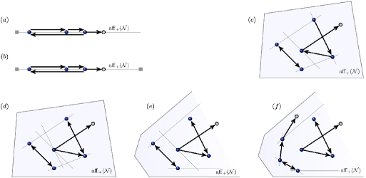
Fig. 3: Examples of lower-endotactic networks - (a), (c), (e) and non lower-endotactic networks - (b), (d), (f).

Affine transformations of reaction networks. An important observation that is used often throughout this paper is that projections of lower-endotatic networks are also lower-endotactic. We prove this fact in the larger context of affine transformations of reaction networks. Let $\mathcal{N}=(\mathcal{S},\mathcal{C},\mathcal{R})$ be a planar reaction network and consider an affine transformation $U:\mathrm{aff}(\mathcal{N})\to\mathbb{R}^{d}$ such that $U(\mathrm{aff}_{+}(\mathcal{N}))\subset\mathbb{R}^{d}_{\geq 0}.$ Similarly to the definition of a projected network, we consider the “generalized” reaction network $U(\mathcal{N}),$ with reactions $U(\mathcal{R})=\{U(P)\to U(P^{\prime})\mid P\to P^{\prime}\in\mathcal{R}\}$ and complexes in the set $U(\mathcal{C})$ which are allowed to have nonnegative real coordinates. We have $\mathrm{aff}_{+}(U(\mathcal{N}))=\mathrm{aff}(U(\mathcal{N}))\cap\mathbb{R}^{d}_{\geq 0}$ and we may ask whether $U(\mathcal{N})$ is lower-endotactic.

Proposition 3.1.

Let $\mathcal{N}$ be a planar reaction network and let $U:\mathrm{aff}(\mathcal{N})\to\mathbb{R}^{d}$ be an affine transformation such that $U(\mathrm{aff}_{+}(\mathcal{N}))\subset\mathbb{R}^{d}_{\geq 0}.$ Then, if $\mathcal{N}$ is lower-endotactic, the planar reaction network $U(\mathcal{N})$ is also lower-endotactic. Moreover, if $\mathcal{N}$ is endotactic, then $U(\mathcal{N})$ is also endotactic.

Proof.

We show the lower-endotactic case; the proof for the endotactic case is similar. Also, we assume that $U$ has rank two; a simpler version of the argument below works if $U$ has rank one. Let ${\bf w}\in\mathrm{iv(aff}_{+}(U(\mathcal{N}))),$ and let $L=esupp^{\bf w}(U(\mathcal{N})).$ Since $U$ takes parallel lines to parallel lines, there exists a vector $\bf v$ such that $U^{-1}(L)=esupp^{\bf v}(\mathcal{N})$ and

$$esupp^{\bf w}(U(\mathcal{N}))_{<0}=U(esupp^{\bf v}(\mathcal{N}))_{<0}).$$

Because $U(\mathrm{aff}_{+}(\mathcal{N}))\subseteq\mathrm{aff}_{+}(U(\mathcal{N})),$ we have $\mathrm{iv(aff}_{+}(U(\mathcal{N})))\subseteq\mathrm{iv}(U(\mathrm{aff}_{+}(\mathcal{N})))$ and therefore ${\bf w}\in\mathrm{iv}(U(\mathrm{aff}_{+}(\mathcal{N}))$. It follows that ${\bf v}\in\mathrm{iv}(\mathrm{aff}_{+}(\mathcal{N})).$ Then, if $U(P)\to U(P^{\prime})\in U(\mathcal{R})$ such that $U(P)\in esupp^{\bf w}(U(\mathcal{N}))$ and $U(P^{\prime})\in esupp^{\bf w}(U(\mathcal{N}))_{<0}$ then $P\to P^{\prime}\in\mathcal{R},$ $P\in esupp^{\bf v}(\mathcal{N})$ and $P^{\prime}\in esupp^{\bf v}(\mathcal{R})_{<0},$ contradicting the fact that $\mathcal{N}$ is lower-endotactic. ∎

4 2D-reduced mass-action systems

A key ingredient in the proof of our main persistence result consists of studying projections of trajectories of $\kappa$-variable mass-action systems onto well-chosen two-dimensional subspaces of $\mathbb{R}^{n}.$ These special projected trajectories obey a specific type of dynamics which we call 2D-reduced mass-action. In this section we show that bounded forward trajectories of such dynamical systems are persistent. To this end we will extend significantly the ideas from [10], where they were introduced in the context of two-species $\kappa$-variable mass-action systems.

4.1 Definition and comparison of reaction rates

Fix an integer $n\geq 2$ and let $l,k$ be two fixed elements of $\{1,\ldots,n\}$ such that $l<k.$ Let $p_{i},\ q_{i}$ be nonnegative rational numbers for $i\in\{1,\ldots,n\}$ such that, for any $i,$ not both $p_{i}$ and $q_{i}$ are zero, and such that $p_{l}=q_{k}=1$ and $p_{k}=q_{l}=0.$ Denote

$$\Psi=\left(\setcounter{MaxMatrixCols}{11}\begin{matrix}p_{1}&\ldots&p_{l-1}&1&p_{l+1}&\ldots&p_{k-1}&0&p_{k+1}&\ldots&p_{n}\\ q_{1}&\ldots&q_{l-1}&0&q_{l+1}&\ldots&q_{k-1}&1&q_{k+1}&\ldots&q_{n}\\ \end{matrix}\right)^{t}.$$ (10)

Definition 20.

Let $\Psi$ be a matrix of the form (10).

(i) Let $\mathcal{N}=(\mathcal{S},\mathcal{C},\mathcal{R})$ be a reaction network with two species, let $\kappa:\mathbb{R}_{\geq 0}\to\mathbb{R}_{>0}^{\mathcal{R}}$ be a piecewise differentiable function and let $a\in\mathbb{R}^{n}.$ For all reactions $P\to P^{\prime}\in\cal R,$ we define $K_{P\to P^{\prime}}:\mathbb{R}_{\geq 0}\times\mathbb{R}^{2}_{\geq 0}\to\mathbb{R}_{\geq 0},$

$$K_{P\to P^{\prime}}(t,{\bf x})=\kappa_{P\to P^{\prime}}(t)(\Psi{\bf x})^{\Psi P+a}.$$ (11)

The reaction system $(\mathcal{N},K)$ is called a 2D-reduced planar mass-action system and is denoted by $(\mathcal{N},\Psi,\kappa,a).$

(ii) For each $s\in\{1,\ldots,p\},$ let $\mathcal{N}_{s}=(\mathcal{S},\mathcal{C}_{s},\mathcal{R}_{s})$ be a two-species reaction network and let $(\mathcal{N}_{s},\Psi,\kappa_{s},a_{s})$ be a 2D-reduced mass-action system. The sum $(\mathcal{N},K)=\bigcup_{s=1}^{p}(\mathcal{N}_{s},\Psi,\kappa_{s},a_{s})$ (recall Definition 7) is called a 2D-reduced mass-action system.

Therefore the concentration vector $c(t)=(x(t),y(t))$ of a 2D-reduced mass-action system $\bigcup_{s=1}^{p}(\mathcal{N}_{s},\Psi,\kappa_{s},a_{s})$ satisfies the following differential equation:

$$\dot{c}(t)=\sum_{s=1}^{p}\sum_{P\to P^{\prime}\in\mathcal{R}_{s}}\kappa_{s,P\to P^{\prime}}(t)(\Psi c(t))^{\Psi P+a_{s}}(P^{\prime}-P).$$ (12)

Note that, by definition, $\kappa$ needs not be bounded away from zero and infinity, as is the case for $\kappa$-variable mass-action systems. However, we will require this condition to prove persistence of 2D-reduced mass-action systems in Corollary 4.1.

The goal of this section is to study the persistence of 2D-reduced mass-action systems. One important component of our analysis is highlighting the reaction whose rate at time $t\geq 0$ “dominates” the other reaction rates. In view of (11) we then consider, for $A>0$ and for any $s\in\{1,\ldots,p\},$ the sign of the difference

$$(\Psi{\bf x})^{\Psi P+a_{s}}-A(\Psi{\bf x})^{\Psi P^{\prime}+a_{s}},$$ (13)

for all pairs of distinct source complexes $P,\ P^{\prime}$ of $\mathcal{N}_{s}.$ For simplicity, and without loss of generality, we assume that $k=2$ and $l=1.$ Then (13) has the same sign as the following expression, which we denote by $\Lambda_{\alpha,\beta}^{A}(x,y):$

$$\Lambda^{A}_{\alpha,\beta}(x,y)=x^{\alpha}y^{-\beta}(p_{3}x+q_{3}y)^{p_{3}\alpha-q_{3}\beta}\ldots(p_{n}x+q_{n}y)^{p_{n}\alpha-q_{n}\beta}-A^{D}.$$ (14)

Here $(\alpha,-\beta)=D(P-P^{\prime})$ and $D$ denotes the least common denominator of all nonzero $p_{i}$ and $q_{i}$, $i\in\{3,\ldots,n\}.$ Note that all the exponents in (14) are integers.

The geometry of the curves $\Lambda^{A}_{\alpha,\beta}(x,y)=0$ within $\mathbb{R}_{>0}^{2}$ is very relevant to our discussion. An immediate goal, which we pursue next, is to find simple approximations for these curves. We will see that within appropriate subsets of $\mathbb{R}_{>0}^{2},$ $\Lambda^{A}_{\alpha,\beta}(x,y)=0$ may be approximated by power curves $y=Cx^{\tau}$ that are ordered in a useful way, as we will explain later in the paper. Let

$$\overline{\Delta}=\left(1+\sum_{i=3}^{n}p_{i}\right)\alpha,\ \overline{\overline{\Delta}}=\left(1+\sum_{i=3}^{n}q_{i}\right)\beta\text{ and }\Delta=\overline{\Delta}-\overline{\overline{\Delta}}.$$ (15)

Lemma 21.

Suppose $\Delta\neq 0.$

(i) If $\alpha\beta<0$ then for all $x>0$ there exists a unique $y>0$ such that $\Lambda^{A}_{\alpha,\beta}(x,y)=0.$

(ii) If $\alpha\beta>0$ then for all small enough $x>0$ there exists a unique $y>0$ such that $\Lambda^{A}_{\alpha,\beta}(x,y)=0.$

Proof.

(i) If $\alpha\beta<0,$ without loss of generality we may take $\alpha>0$ and $\beta<0.$ For any fixed $x>0,$ $\Lambda_{\alpha,\beta}^{A}(x,y)$ is a polynomial in $y$ whose coefficients are all positive, except for its free term $-A^{D}.$ The Descartes rule of signs implies that this polynomial has a unique positive root.

(ii) If $\alpha\beta>0,$ we may assume that $\alpha>0$ and $\beta>0.$ $\Lambda^{A}_{\alpha,\beta}(x,y)=0$ implies

$$A^{D}y^{\beta}(p_{3}x+q_{3}y)^{q_{3}\beta}\ldots(p_{n}x+q_{n}y)^{q_{n}\beta}=x^{\alpha}(p_{3}x+q_{3}y)^{p_{3}\alpha}\ldots(p_{n}x+q_{n}y)^{p_{n}\alpha}.$$ (16)

We rewrite this equality by excluding the factors of zero power and merging the powers of $x$ in the left hand side and the powers of $y$ in right hand side. We denote

$$\lambda_{x}=1+\sum_{\begin{subarray}{c}{i\in\{3,\ldots,n|}\\ {q_{i}=0\}}\end{subarray}}p_{i}\quad\text{ and }\lambda_{y}=1+\sum_{\begin{subarray}{c}{i\in\{3,\ldots,n|}\\ {p_{i}=0\}}\end{subarray}}q_{i},$$ (17)

and we let $i_{l}$, $l\in\{1,\ldots,I\}$ be the indices for which both $p_{i_{l}}$ and $q_{i_{l}}$ are strictly positive. Then we have

$$A^{\prime}y^{\lambda_{y}\beta}(p_{i_{1}}x+q_{i_{1}}y)^{q_{i_{1}}\beta}\ldots(p_{i_{I}}x+q_{i_{I}}y)^{q_{i_{I}}\beta}-x^{\lambda_{x}\alpha}(p_{i_{1}}x+q_{i_{1}}y)^{p_{i_{1}}\alpha}\ldots(p_{i_{I}}x+q_{i_{I}}y)^{p_{i_{I}}\alpha}=0$$ (18)

where $A^{\prime}=A^{D}\prod_{i\in\{1,\ldots,n\}\backslash\{i_{1},\ldots,i_{I}\}}q_{i}^{q_{i}\beta}p_{i}^{-p_{i}\alpha}.$ We denote the polynomial in (18) by $F(x,y).$

If $\lambda_{y}\beta>\overline{\Delta}-\lambda_{x}\alpha$ then equation (18) yields

$$F(x,y) = \overline{\overline{C}}_{0}y^{\overline{\overline{\Delta}}}+(\overline{\overline{C}}_{1}\ x)y^{\overline{\overline{\Delta}}-1}+\ldots+(\overline{\overline{C}}_{\overline{\overline{\Delta}}-\lambda_{y}\beta}\ x^{\overline{\overline{\Delta}}-\lambda_{y}\beta})y^{\lambda_{y}\beta}$$

$$- (\overline{C}_{\lambda_{x}\alpha}x^{\lambda_{x}\alpha})y^{\overline{\Delta}-\lambda_{x}\alpha}-(\overline{C}_{\lambda_{x}\alpha+1}\ x^{\lambda_{x}\alpha+1})y^{\overline{\Delta}-\lambda_{x}\alpha-1}-(\overline{C}_{\overline{\Delta}-1}\ x^{\overline{\Delta}-1})y-\overline{C}_{\overline{\Delta}}\ x^{\overline{\Delta}}=0,$$

where the coefficients $\overline{\overline{C}}_{k}$ and $\overline{C}_{k}$ are positive and are obtained from expanding the first, respectively second term of the difference (18), and if $\lambda_{y}\beta\leq\overline{\Delta}-\lambda_{x}\alpha$ we have

$$F(x,y) = \overline{\overline{C}}_{0}y^{\overline{\overline{\Delta}}}+(\overline{\overline{C}}_{1}\ x)y^{\overline{\overline{\Delta}}-1}+\ldots+(\overline{\overline{C}}_{\overline{\overline{\Delta}}-(\overline{\Delta}-\lambda_{x}\alpha+1)}\ x^{\overline{\overline{\Delta}}-(\overline{\Delta}-\lambda_{x}\alpha+1)})y^{\overline{\Delta}-\lambda_{x}\alpha+1}+$$

$$+ (\overline{\overline{C}}_{\overline{\overline{\Delta}}-(\overline{\Delta}-\lambda_{x}\alpha)}\ x^{\overline{\overline{\Delta}}-(\overline{\Delta}-\lambda_{x}\alpha)}-\overline{C}_{\lambda_{x}\alpha}x^{\lambda_{x}\alpha})y^{\overline{\Delta}-\lambda_{x}\alpha}+\ldots$$

$$+ (\overline{\overline{C}}_{\overline{\overline{\Delta}}-\lambda_{y}\beta}\ x^{\overline{\overline{\Delta}}-\lambda_{y}\beta}-\overline{C}_{\overline{\Delta}-\lambda_{y}\beta}\ x^{\overline{\Delta}-\lambda_{y}\beta})y^{\lambda_{y}\beta}$$

$$- (\overline{C}_{\overline{\Delta}-(\lambda_{y}\beta-1)}\ x^{\overline{\Delta}-(\lambda_{y}\beta-1)})y^{\lambda_{y}\beta-1}-\ldots-(\overline{C}_{\overline{\Delta}-1}\ x^{\overline{\Delta}-1})y-\overline{C}_{\overline{\Delta}}\ x^{\overline{\Delta}}=0.$$

In the first case, for any fixed $x>0,$ the coefficients of $F_{x}(y)=F(x,y)$ viewed as a polynomial in $y$ change sign exactly once. It follows from the Descartes rule of signs that $F_{x}(y)=0$ has a unique positive solution. In the second case, the coefficients of $F_{x}(y)$ that are binomials in $x$ are of the form $\overline{\overline{C}}x^{\overline{\overline{\Delta}}-k}-\overline{C}x^{\overline{\Delta}-k}$ and for small $x$ are all either positive if $\overline{\overline{\Delta}}<\overline{\Delta}$ or negative if $\overline{\overline{\Delta}}>\overline{\Delta}.$ Therefore for small enough $x$ the polynomial $F_{x}(y)$ changes the sign of its coefficients only once either at $y^{\overline{\Delta}-\lambda_{x}\alpha}$ if $\Delta<0$ or at $y^{\lambda_{y}\beta-1}$ if $\Delta>0$. It follows that the equation $F_{y}(x)=0$ a unique positive solution. ∎

Remark 4.1.

Lemma 21 implies that for $\alpha\beta<0,$ the curve $\{(x,y)\in\mathbb{R}_{>0}^{2}\mid\Lambda^{A}_{\alpha,\beta}(x,y)=0\}$ is the graph of a function $y^{A}_{\alpha,\beta}:\mathbb{R}_{>0}\to\mathbb{R}_{>0}.$ It is easy to see that $\lim_{x\to 0}y^{A}_{\alpha,\beta}(x)=\infty\text{ and }\lim_{x\to\infty}y^{A}_{\alpha,\beta}(x)=0.$ On the other hand, if $\alpha\beta>0,$ the function $y^{A}_{\alpha,\beta}$ is defined only for small $x>0$: there exists $M_{\alpha,\beta}^{A}>0$ such that $\{(x,y)\in(0,M_{\alpha,\beta}^{A})\times\mathbb{R}_{>0}\mid\Lambda^{A}_{\alpha,\beta}(x,y)=0\}$ is the graph of $y^{A}_{\alpha,\beta}:(0,M_{\alpha,\beta}^{A})\to\mathbb{R}_{>0}.$ We claim that in this case we have $\lim_{x\to 0}y_{\alpha,\beta}^{A}=0.$ Indeed, suppose $\Delta<0.$ If for some $0\leq l<\infty,$ $(0,l)$ is a limit point of the curve $\{(x,y)\in\mathbb{R}^{2}_{>0}\mid\Lambda^{A}_{\alpha,\beta}(x,y)=0\},$ then plugging $(0,l)$ into (18) yields $l=0.$ It remains to check that $(0,\infty)$ is not a limit point of the curve above. If $\{(x_{n},y_{n})\}_{n>0}$ is a sequence of points with positive coordinates such that $\lim_{n\to\infty}(x_{n},y_{n})=(0,\infty)$ and $\Lambda^{A}_{\alpha,\beta}(x_{n},y_{n})=0,$ from (18) we get $\mathcal{O}(x_{n}^{\lambda_{x}\alpha})=\mathcal{O}(y_{n}^{-\Delta+\lambda_{x}\alpha})$ as $n\to\infty,$ which contradicts $\Delta<0.$ The case $\Delta>0$ follows from symmetry.

Lemma 22.

Suppose $\alpha\beta>0.$

(i) If $\Delta=0$ there exist positive constants $\gamma^{A}_{\alpha,1},\ldots,\gamma^{A}_{\alpha,N}$ for some integer $N>1$ such that

$$\Lambda^{A}_{\alpha,\beta}(x,y)=0\text{ for some }(x,y)\in\mathbb{R}_{>0}^{2}\text{ if and only if }y=\gamma^{A}_{\alpha,i}x\text{ for some }i\in\{1,\ldots,N\}.$$

(ii) If $\Delta\neq 0$ there exists a strictly increasing function $\tau:\mathbb{R}_{>0}\to\mathbb{R}_{>0}$ such that, for function $y_{\alpha,\beta}^{A}$ introduced in Remark 4.1, the limit

$$\lim_{x\to 0}\frac{y^{A}_{\alpha,\beta}(x)}{x^{\tau(\alpha/\beta)}}$$

exists, is positive and finite. We denote this limit by $C^{A}_{\alpha,\beta}.$

Proof.

$(i).$ Dividing (18) by $x^{\overline{\Delta}}=x^{\overline{\overline{\Delta}}}$ and letting $\gamma=y/x$ yields

$$A^{\prime}\gamma^{\lambda_{y}\beta}(p_{i_{1}}+q_{i_{1}}\gamma)^{q_{i_{1}}\beta}\ldots(p_{i_{I}}+q_{i_{I}}\gamma)^{q_{i_{I}}\beta}-(p_{i_{1}}+q_{i_{1}}\gamma)^{p_{i_{1}}\alpha}\ldots(p_{i_{I}}+q_{i_{I}}\gamma)^{p_{i_{I}}\alpha}=0.$$

We denote by $\overline{F}(\gamma)$ the polynomial above. The positive term in the expression of $\overline{F}$ has degree $\overline{\Delta},$ and the negative term has degree $\overline{\Delta}-\lambda_{x}\alpha,$ therefore $\lim_{\gamma\to\infty}\overline{F}(\gamma)=\infty.$ Since $\overline{F}(0)<0,$ there exists at least one positive root of $\overline{F}.$ Denoting the positive roots of $\overline{F}$ by $\gamma^{A}_{\alpha,1},\ldots,\gamma^{A}_{\alpha,N}$ completes the proof.

$(ii)$ We know from see Remark 4.1 that $(0,0)$ is a limit point of $\{(x,y)\in\mathbb{R}_{>0}^{2}\mid\Lambda_{\alpha,\beta}^{A}(x,y)=0\}.$ Lemma 21 implies that this curve has a unique Puiseux expansion in a neighborhood of $(0,0)$ (see [28] for a discussion of Puiseux expansions). By making $M_{\alpha,\beta}^{A}$ from Remark 4.1 as small as necessary for the Puiseux expansion to hold in $x\in(0,M_{\alpha,\beta}^{A})$, we have, for all $x\in(0,M_{\alpha,\beta}^{A})$:

$$y_{\alpha,\beta}^{A}(x)=C_{\alpha,\beta}^{A}x^{T}+\text{ higher order terms in }x$$ (19)

where $C_{\alpha,\beta}^{A}\in\mathbb{R}$ and $T>0$ is a rational number. The exponent $T$ in (19) is equal to the negative of one of the slopes in the lower boundary of the Newton polygon of the polynomial $F(x;y)$ defined in (18); (see [28] for more details).

Fig. 4: Monomials of $F(x;y)$ (see 18). The lattice point $(a,b)$ represents the monomial $x^{b}y^{a}$ and the lower boundary of negative slope of the associated Newton polygon is the thick polygonal line. The picture on the left corresponds to $\Delta>0$ and the one on the right corresponds to $\Delta<0.$

Since $F$ is the difference of two homogeneous polynomials of degrees $\overline{\Delta}$ and $\overline{\overline{\Delta}},$ its Newton polygon can be easily illustrated (see Figure 4) and the slopes of its lower boundary are

$$\left\{-1,-\frac{\overline{\Delta}-(\overline{\overline{\Delta}}-\lambda_{y}\beta)}{\lambda_{y}\beta}\right\}\text{ or }\left\{-1,-\frac{\lambda_{x}\alpha}{\overline{\overline{\Delta}}-(\overline{\Delta}-\lambda_{x}\alpha)}\right\}$$ (20)

if $\Delta>0$ or $\Delta<0,$ respectively. Note that $T$ cannot be equal to one, for otherwise from (18) it would follow that $\mathcal{O}(x^{\overline{\Delta}})=\mathcal{O}(x^{\overline{\overline{\Delta}}})$, contradicting $\overline{\Delta}\neq\overline{\overline{\Delta}};$ therefore $-T$ is given by the fractions in (20). Then, if we define the function $\tau:\mathbb{R}_{>0}\to\mathbb{R}_{>0}$ as follows:

$$\tau(\sigma)=\begin{cases}\lambda_{x}\left(\displaystyle\frac{1}{\sigma}\displaystyle\sum_{i=1}^{n}q_{i}-\sum_{i=1}^{n}p_{i}\right)^{-1},&\text{ if }\displaystyle\sigma<\sum_{i=1}^{n}q_{i}/\sum_{i=1}^{n}p_{i},\\ 1,&\text{ if }\displaystyle\sigma=\sum_{i=1}^{n}q_{i}/\sum_{i=1}^{n}p_{i},\\ \displaystyle{\frac{1}{\lambda_{y}}}\left(\sigma\sum_{i=1}^{n}p_{i}-\sum_{i=1}^{n}q_{i}\right),&\text{ if }\displaystyle\sigma>\sum_{i=1}^{n}q_{i}/\sum_{i=1}^{n}p_{i},\end{cases}$$

we can easily see that $T=\tau(\alpha/\beta).$ Note that $\tau$ is continuous and strictly increasing. Moreover, the value of $\sigma$ for which $\tau(\sigma)=1$ corresponds to $\Delta=0$, and thus the statement in part $(i)$ of the lemma is incorporated in part $(ii).$ ∎

4.2 The domination lemma

The following key result reinforces our motivation for considering differences (13) of reaction rates. Roughly speaking, it shows that if, at time $t,$ the rate of a reaction $P^{\prime}_{0}\to P_{0}$ dominates all the other reaction rates, then the reaction vector $P^{\prime}_{0}-P_{0}$ “dictates” the direction of the flow $\dot{c}(t).$

Lemma 23.

Let $(\mathcal{N},K)=(\mathcal{S},\mathcal{C},\mathcal{R},K)$ be a reaction system, let $P_{0}\to P^{\prime}_{0}\in{\mathcal{R}}$ and let $\bf{v}$ be a vector such that $(P^{\prime}_{0}-P_{0})\cdot{\bf v}>0.$ Also let $\mathcal{U}\subseteq\mathcal{SC}(\mathcal{N})\backslash\{P_{0}\}.$ There exists a positive constant $\mu$ such that if for some $(t,{\bf x})\in\mathbb{R}_{\geq 0}\times\mathbb{R}_{\geq 0}^{n}$ we have $K_{P_{0}\to P^{\prime}_{0}}(t,{\bf x})>0$ and

$$K_{P_{0}\to P^{\prime}_{0}}(t,{\bf x})>\mu K_{P\to P^{\prime}}(t,{\bf x})\text{ for all }P\to P^{\prime}\in\mathcal{R}\text{ with }P\in\mathcal{U}$$

then

$$\Bigg{(}K_{P_{0}\to P^{\prime}_{0}}(t,{\bf x})(P^{\prime}_{0}-P_{0})+\sum_{P\to P^{\prime},P\in\mathcal{U}}K_{P\to P^{\prime}}(t,{\bf x})(P^{\prime}-P)\Bigg{)}\cdot{\bf{v}}>0.$$

Proof.

We take

$$\mu=\frac{\parallel{\bf v}\parallel\displaystyle\sum_{P\to P^{\prime}\in\mathcal{R}}\parallel P-P^{\prime}\parallel}{(P^{\prime}_{0}-P_{0})\cdot\bf{v}}$$

and we have

$$\Bigg{(}K_{P^{\prime}_{0}\to P_{0}}(t,{\bf x})(P^{\prime}_{0}-P_{0})+\sum_{P\to P^{\prime},P\in\mathcal{U}}K_{P\to P^{\prime}}(t,{\bf x})(P^{\prime}-P)\Bigg{)}\cdot{\bf{v}}$$

$$>K_{P_{0}\to P^{\prime}_{0}}(t,{\bf x})(P^{\prime}_{0}-P_{0})\cdot{\bf v}-\sum_{P\to P^{\prime},P\in\mathcal{U}}\Bigg{(}(1/\mu)K_{P_{0}\to P^{\prime}_{0}}(t,{\bf x})\parallel{\bf v}\parallel\parallel P-P^{\prime}\parallel\Bigg{)}$$

$$\geq\left((P^{\prime}_{0}-P_{0})\cdot{\bf{v}}-(1/\mu)\parallel{\bf v}\parallel\sum_{P\to P^{\prime}\in\mathcal{R}}\parallel P^{\prime}-P\parallel\right)K_{P_{0}\to P^{\prime}_{0}}(t,{\bf x})=0,$$

where the first inequality was obtained using the Cauchy-Schwarz inequality. ∎

Remark 4.2.

If $(\mathcal{S},\mathcal{C},\mathcal{R},\Psi,\kappa,a)$ is a 2D-reduced planar mass-action system and if $\kappa(t)\in(\eta,1/\eta)^{\mathcal{R}}$ for some $t\geq 0$ then $K_{P\to P^{\prime}}(t,{\bf x})=\kappa_{P\to P^{\prime}}(t)(\Psi{\bf x})^{\Psi P+a},$ and therefore $(\Psi{\bf x})^{\Psi P_{0}+a}>(\mu/\eta^{2})(\Psi{\bf x})^{\Psi P+a}$ implies $K_{P_{0}\to P^{\prime}_{0}}(t,{\bf x})>\mu K_{P\to P^{\prime}}(t,{\bf x})$, which is exactly the condition needed in Lemma 23. Or, using the notation in (14) and letting $(\alpha,-\beta)=D(P_{0}-P):$

$$\Lambda^{\mu/\eta^{2}}_{\alpha,\beta}({\bf x})>0\text{ implies }K_{P_{0}\to P^{\prime}_{0}}(t,{\bf x})>\mu K_{P\to P^{\prime}}(t,{\bf x}).$$ (21)

4.3 Geometric constructions in the phase plane

Our strategy for proving that a trajectory $T(c_{0})$ of a certain reaction system is persistent relies on building a convex set $\mathcal{L}^{+}\subset\mathbb{R}^{2}_{>0}$ that contains $T(c_{0})$ and stays away from $\partial\mathbb{R}^{2}_{\geq 0}.$ As in [10], we partition the phase plane into subsets where one reaction rate dominates all the others, and therefore, by Lemma 23, its corresponding reaction vector dictates the direction of the vector field. The set $\mathcal{L}^{+}$ is constructed such that, on each subset of the partition, the dominating reaction vector (and therefore, by Lemma 23, the vector field), points towards the interior of $\mathcal{L}^{+}$. This is the rather simple idea behind the proof of Theorem 4.1, but the technical details involved are quite delicate. We start with the construction of the set $\mathcal{L}^{+}$, which is discussed next.

For any $s\in\{1,\ldots,p\},$ let $\mathcal{N}_{s}=(\mathcal{S},\mathcal{C}_{s},\mathcal{R}_{s})$ be a lower-endotactic two-species reaction network and let $(\mathcal{N},K)=\bigcup_{s=1}^{p}(\mathcal{N}_{s},\kappa_{s},\Psi,a_{s})$ be a 2D-reduced mass-action system. We also let $\eta<1$ be a positive constant. Let $D$ denote the least common denominator of all nonzero elements of $\Psi.$ For each $s\in\{1,\ldots,p\}$ let

$$\{r^{s}_{1},\ldots,r^{s}_{e(s)}\}=\big{\{}\alpha/\beta\mid(\alpha,-\beta)\in\{D(P-P^{\prime})\mid P,P^{\prime}\in{\mathcal{SC}}(\mathcal{N}_{s}),\alpha\beta>0\}\big{\}};$$

we assume that $r_{1}^{s}<\ldots<r_{e(s)}^{s}$ and define the set

$${\bf V}=\{(1,\tilde{r}_{1}),\ldots,(1,\tilde{r}_{e})\}=\bigcup_{s=1}^{p}\{(1,r^{s}_{i})\mid i\in\{1,\ldots,e(s)\}\}$$ (22)

where we take $\tilde{r}_{1}<\ldots<\tilde{r}_{e}.$ Let $\{\bf i,j\}$ be the standard basis of the cartesian plane. Since $\mathcal{N}_{s}$ is endotactic, for each $s\in\{1,\ldots,p\}$ and for all vectors $\bf n\in{\bf V}\cup\{\bf i,\bf j\},$ there exists a reaction

$$P_{s,\bf n}\to P^{\prime}_{s,\bf n}\in\mathcal{R}_{s}\text{ such that }P_{s,\bf n}\in esupp^{\bf n}(\mathcal{N}_{s})\text{ and }P^{\prime}_{s,\bf n}\in esupp^{\bf n}(\mathcal{N}_{s})_{>0}.$$ (23)

Note that there might exist multiple reactions as in (23), out of which $P_{s,\bf n}\to P^{\prime}_{s,\bf n}$ is chosen and fixed for the remaining of this paper.

If $\mu_{{\bf n},s}$ denotes the constant from Lemma 23 that corresponds to reaction $P_{s,\bf n}\to P^{\prime}_{s,\bf n}$ $\bf v=\bf n$ and $\mathcal{U}=\mathcal{SC(N}_{s})\cap esupp^{\bf n}(\mathcal{N}_{s})_{>0}$ we define

$$\mu=\max\big{\{}\mu_{{\bf n},s}\mid{\bf n}\in{\bf V}\cup\{{\bf i,j}\},s\in\{1,\ldots,p\}\big{\}}.$$ (24)

We also let

$$\mathcal{D}=\bigcup_{s=1}^{p}\{D(P-P^{\prime})\mid P,P^{\prime}\in\mathcal{SC(N}_{s})\},$$

and finally, inspired by Remark 4.2, we denote $A=\mu/\eta^{2}.$

Let $M>1$ be a fixed number. We choose $0<\delta<1$ and $0<\xi<1$ to satisfy the following properties:

• (P1)	$\delta<\displaystyle\frac{1}{2}\min\{C_{\alpha,\beta}^{A},\gamma_{\alpha,i}^{A}\mid(\alpha,-\beta)\in{\mathcal{D}},\alpha\beta>0\}$,
  	$\displaystyle\frac{1}{\delta}>\frac{3}{2}\max\{C_{\alpha,\beta}^{A},\gamma_{\alpha,i}^{A}\mid(\alpha,-\beta)\in{\mathcal{D}},\alpha\beta>0\}$

  where $C_{\alpha,\beta}^{A}$ and $\gamma_{\alpha,i}^{A}$ are defined in Lemma 22;
  (P2) all pairwise intersections from the strictly positive quadrant of the $2e$ curves $y=\delta x^{\tau(\tilde{r}_{i})},\ y=(1/\delta)x^{\tau(\tilde{r}_{i})},$ $i\in\{1,\ldots,e\},$ lie in $(\xi,\infty)^{2}$;
  (P3) the square $[0,\xi]^{2}$ lies below the curves $\Lambda_{\alpha,\beta}^{A}(x,y)=0$ for all $(\alpha,-\beta)\in{\mathcal{D}}\text{ with }\alpha\beta\leq 0;$
  (P4) for all $(\alpha,-\beta)\in\mathcal{D}$ such that $\alpha\beta>0$ we have $\xi<M^{A}_{\alpha,\beta}$ (recall that $M^{A}_{\alpha,\beta}$ is such that $y_{\alpha,\beta}^{A}:(0,M_{\alpha,\beta}^{A})$ admits a Puiseux series representation), and for all $x\in(0,\xi]$ we have

  $$\frac{1}{2}C^{A}_{\alpha,\beta}x^{\tau(\alpha/\beta)}<y^{A}_{\alpha,\beta}(x)<\frac{3}{2}C^{A}_{\alpha,\beta}x^{\tau(\alpha/\beta)}.$$

  
  

Fig. 5: Construction of $\mathcal{L}^{+}.$ Each dashed line represents a curve $\Lambda^{A}_{\alpha,\beta}=0$ in the positive quadrant and is labeled with a relation that the corresponding $\alpha$ and $\beta$ satisfy. The curves $y=\delta x^{\tau(\tilde{r}_{i})}$ and $y=(1/\delta)x^{\tau(\tilde{r}_{i})}$ are depicted using solid lines. The highlighted area represents the set $\mathcal{L}^{+}.$

Clearly, $\xi$ can be chosen small enough so that (P2) and (P3) are satisfied (see Figure 5). The existence of $\xi$ that also satisfies (P4) is a consequence of Lemma 22. Since $\tau$ is a strictly increasing function, condition (P2) implies that for $x\in(0,\xi]$ we have

$$(1/\delta)x^{\tau(\tilde{r}_{i+1})}<\delta x^{\tau(\tilde{r}_{i})}\text{ for all }i\in\{1,\ldots,e-1\}.$$

Moreover, for $x<\xi,$ (P1) and (P4) imply that for $\alpha\beta>0$ the curve $\{(x,y)\in\mathbb{R}_{>0}^{2}\mid\Lambda^{A}_{\alpha,\beta}(x,y)=0\}$ lies between the curves $\delta x^{\tau(\alpha/\beta)}$ and $(1/\delta)x^{\tau(\alpha/\beta)}$ (see Figure 5).

Now, for the actual construction of $\mathcal{L}^{+},$ first assume that ${\bf V}\neq\O$ and start with a point $A_{0}\in\{0\}\times(0,\xi]$ on the $y$ axis. We choose a point $A_{2}$ between the curves $y=(1/\delta)x^{\tau(\tilde{r}_{2})}$ and $y=\delta x^{\tau(\tilde{r}_{1})}$ such that the slope of the line $A_{0}A_{2}$ is $-1/\tilde{r}_{1}.$ Inductively, choose points $A_{i+1},\ i\in\{2,\ldots,e-1\}$ such that

$$(i)\ \text{ the point }A_{i+1}\text{ lies between the curves }y=(1/\delta)x^{\tau(\tilde{r}_{i+1})}\text{ and }y=\delta x^{\tau(\tilde{r}_{i})}$$

$$(ii)\text{ the line }A_{i}A_{i+1}\text{ has slope }-1/\tilde{r}_{i}.$$

Finally, $A_{e+2}$ is defined on the $x$ axis such that $A_{e}A_{e+2}$ has slope $-1/\tilde{r}_{e}.$

The polygonal line $[A_{0}A_{2}A_{3}\ldots A_{e-1}A_{e}A_{e+2}]$ is convex. We move $A_{0}$ closer to the origin if necessary, such that all the points $A_{i}$ defined above lie in the square $(0,\xi]^{2}.$

If ${\bf V}=\O$ we let $A_{0}$ and $A_{3}$ be two points on the $y$ and $x$ axes, respectively, such that $A_{0},\ A_{3}\in[0,\xi]^{2}$ and the slope of the line $A_{0}A_{3}$ is -1.

The last step of the construction consists of defining $d$ small enough such that (P5) and (P6) below are satisfied:

• (P5) If ${\bf V}\neq\O$ then the vertical half-line $\{d\}\times[0,\infty)$ intersects the segment $A_{0}A_{2}$ at a point $A_{1}$ above the curve $y=(1/\delta)x^{\tau(\tilde{r}_{1})}$; also, the horizontal half-line $[0,\infty)\times\{d\}$ intersects the segment $A_{e}A_{e+2}$ at a point $A_{e+1}$ below the curve $y=\delta x^{\tau(\tilde{r}_{e})}.$ If ${\bf V}=\O$ then $d$ is chosen such that $d<\xi/2,$ and the intersection of the vertical half-line $\{d\}\times[0,\infty)$ with the segment $A_{0}A_{3}$ is denoted $A_{1},$ whereas the intersection of the horizontal half-line $[0,\infty)\times\{d\}$ with the segment $A_{0}A_{3}$ is denoted $A_{2};$

  (P6)	$\Lambda^{A}_{\alpha,\beta}(d,M)>0\text{ for }(\alpha,-\beta)\in{\mathcal{D}},\alpha<0,\beta\geq 0,$
  	$\Lambda^{A}_{\alpha,\beta}(M,d)>0\text{ for }(\alpha,-\beta)\in{\mathcal{D}},\alpha\geq 0,\beta<0;$

Recall that $M>1$ was fixed at the beginning of the construction. It is easy to see that (14) implies that (P6) holds for $d$ small enough.

Let

$$\mathcal{L}=\{A_{1}+(0,t)\mid t\geq 0\}\cup[A_{1}\ldots A_{e+1}]\cup\{A_{e+1}+(t,0)\mid t\geq 0\}$$

be made out of the polygonal line $[A_{1}\ldots A_{e}],$ (called, for future reference, the finite part of $\mathcal{L}$) completed with a vertical and a horizontal half-lines (the union of which we call the infinite part of $\mathcal{L}$). Finally, we define $\mathcal{L}^{+}=\mathrm{conv}(\mathcal{L}).$

To indicate the quantities that $\mathcal{L}^{+}$ depends on, we write $\mathcal{L}^{+}=\mathcal{L}^{+}(\{\mathcal{N}_{s}\}_{1\leq s\leq p},\Psi,\eta,M).$ The polygonal line $[A_{0},\ldots,A_{e+2}]$ will also be useful later in this paper. We denote it by $\overline{\mathcal{L}}=\overline{\mathcal{L}}(\{\mathcal{N}_{s}\}_{1\leq s\leq p},\Psi,\eta)$ (note that $M$ is not required for $\overline{\mathcal{L}}$) and we let $\overline{\mathcal{L}}^{+}$ be the unbounded part of $\mathbb{R}^{2}_{\geq 0}$ that is delimited by $\overline{\mathcal{L}}.$

4.4 Persistence of 2D-reduced mass-action systems

The following theorem is the main result of this section.

Theorem 4.1.

Let $(\mathcal{N},K)=\bigcup_{s=1}^{p}(\mathcal{N}_{s},\kappa_{s},\Psi,a_{s})$ be a 2D-reduced mass-action system where $\mathcal{N}_{s}=(\mathcal{S},\mathcal{C}_{s},\mathcal{R}_{s})$ is lower-endotactic for all $s\in\{1,\ldots,p\}$ and denote

$$f(t,{\bf x})=\sum_{s=1}^{p}\sum_{P\to P^{\prime}\in\mathcal{R}_{s}}\kappa_{s,P\to P^{\prime}}(t)(\Psi{\bf x})^{\Psi P+a_{s}}(P^{\prime}-P).$$

Let $\eta\in(0,1)$ and $M>1$ be real numbers. Then for any $t\geq 0$ such that $\kappa_{s}(t)\in(\eta,1/\eta)^{\mathcal{R}_{s}}$ for all $s\in\{1,\ldots,p\}$, and for any ${\bf x}\in{\mathcal{L}}(\{\mathcal{N}_{s}\}_{1\leq s\leq p},\Psi,\eta,M)\cap[0,M]^{2}$ we have

$${\bf n}\cdot f(t,{\bf x})\geq 0\text{ for all }{\bf n}\in-N_{\mathcal{L}^{+}}(\bf x).$$ (25)

Proof.

The cone $-N_{\mathcal{L}^{+}}({\bf x})$ is degenerate unless ${\bf x}$ is a vertex of $\mathcal{L}$ and its generators belong to $\bf V\cup\{\bf i,j\},$ where $\bf V$ is the set of vectors defined in (22). It then suffices to show that for any $s\in\{1,\ldots,p\}$ and for any ${\bf n}\in-N_{\mathcal{L}^{+}}({\bf x})\cap(\bf V\cup\{i,j\})$ we have

$$\Bigg{(}\sum_{P\to P^{\prime}\in\mathcal{R}_{s,\bf n}}K_{s,P\to P^{\prime}}(t,{\bf x})(P^{\prime}-P)\Bigg{)}\cdot{\bf n}\geq 0$$ (26)

for all $s\in\{1,\ldots,p\},$ where $K_{s,P\to P^{\prime}}(t,{\bf x})=\kappa_{s,P\to P^{\prime}}(t)(\Psi{\bf x})^{\Psi P+a_{s}}$ is the rate of the reaction $P\to P^{\prime}\in\mathcal{R}_{s}$ at time $t.$ We fix $s\in\{1,\ldots,p\}$ and recall that $\mathcal{R}_{s,\bf n}=\{P\to P^{\prime}\in{\mathcal{R}}_{s}\mid(P^{\prime}-P)\cdot{\bf n}\neq 0\}$ denotes the $\bf n$-essential subnetwork of $\mathcal{R}_{s}.$ The inequality (26) is trivially true if $\mathcal{R}_{s,\bf n}=\O.$ Otherwise, recall the reaction $P_{s,\bf n}\to P^{\prime}_{s,\bf n}\in\mathcal{R}_{s,\bf n}$ from (23). We rewrite the left hand side of (26) by separating the reactions with source on $esupp^{\bf n}(\mathcal{N}_{s})$ and emphasizing the reaction $P_{s,\bf n}\to P^{\prime}_{s,\bf n}:$

$$\Bigg{(}\sum_{P\to P^{\prime}\in\mathcal{R}_{s,\bf n}}K_{s,P\to P^{\prime}}(t,{\bf x})(P^{\prime}-P)\Bigg{)}\cdot{\bf n}=\Bigg{(}\sum_{\begin{subarray}{c}{\{P\to P^{\prime}\in\mathcal{R}_{s,\bf n}}|\\ {P\in esupp^{{\bf n}}(\mathcal{N}_{s})}\\ {P\to P^{\prime}\neq P_{s,\bf n}\to P^{\prime}_{s,\bf n}\}}\end{subarray}}K_{s,P\to P^{\prime}}(t,{\bf x})(P^{\prime}-P)+$$

$$+K_{s,P_{s,\bf n}\to P^{\prime}_{s,\bf n}}(t,{\bf x})(P^{\prime}_{s,\bf n}-P_{s,\bf n})+\sum_{\begin{subarray}{c}{\{P\to P^{\prime}\in\mathcal{N}_{s,\bf n}}|\\ {P\notin esupp^{{\bf n}}(\mathcal{N}_{s})\}}\end{subarray}}K_{s,P\to P^{\prime}}(t,{\bf x})(P^{\prime}-P)\Bigg{)}\cdot{\bf n}.$$

Since all source complexes of $\mathcal{R}_{s,\bf n}$ lie in $esupp^{{\bf n}}({\mathcal{N}}_{s})_{\geq 0}$, the reaction vector $P^{\prime}-P$ with source $P\in esupp^{{\bf n}}(\mathcal{N}_{s})$ satisfies $(P^{\prime}-P)\cdot{\bf n}\geq 0.$ It is therefore enough to show that

$$\Bigg{(}K_{s,P_{s,\bf n}\to P^{\prime}_{s,\bf n}}(t,{\bf x})(P^{\prime}_{s,\bf n}-P_{\bf n})+\sum_{\begin{subarray}{c}{\{P\to P^{\prime}\in\mathcal{R}_{s,\bf n}}|\\ {P\notin esupp^{{\bf n}}(\mathcal{N}_{s})\}}\end{subarray}}K_{s,P\to P^{\prime}}(t,{\bf x})(P^{\prime}-P)\Bigg{)}\cdot{\bf n}\geq 0$$ (27)

in order to verify (26). In turn, (27) will follow from Lemma 23 with $\mathcal{U}=\mathcal{SC(N}_{s})\cap esupp^{{\bf n}}(\mathcal{R}_{s})_{>0}$ and the fact that

$$K_{P_{s,\bf n}\to P^{\prime}_{s,\bf n}}(t,{\bf x})>\mu K_{P\to P^{\prime}}(t,{\bf x})$$ (28)

for all $P\to P^{\prime}\in{\mathcal{R}}_{s}$ with $P\in\mathcal{U}$ (recall $\mu$ from (24)). Therefore showing inequality (28) will complete the proof of the theorem.

As noted in Remark 4.2, (28) is implied by

$$\Lambda^{A}_{\alpha,\beta}({\bf x})>0,$$ (29)

where $(\alpha,-\beta)=D(P_{s,\bf n}-P)$ and $A=\mu/\eta^{2}.$ To verify (29), we consider different cases, according on the location of ${\bf x}=(x,y)$ on $\mathcal{L}.$ First suppose that ${\bf x}$ lies on the line segment $[A_{i}A_{i+1}]$ for some $i\in\{1,\ldots,e\}.$ Then (see Figure 5), if $\tilde{r}_{i^{\prime}}<\tilde{r}_{i}<\tilde{r}_{i^{\prime\prime}}$, or equivalently, if $i^{\prime}<i<i^{\prime\prime}$, we have

$$(1/\delta)x^{\tau(\tilde{r}_{i^{\prime\prime}})}<y<\delta x^{\tau(\tilde{r}_{i^{\prime}})}.$$ (30)

Depending on the sign combination of $\alpha$ and $\beta,$ the source complex $P$ may belong to one of the three shaded regions in Figure 6(a).

Fig. 6: Positions of a source complex $P$ relative to $P_{s,\bf n}$

Region I. Here $\alpha<0$ and $\beta<0$; (29) is equivalent to $y>y^{A}_{\alpha,\beta}(x).$ The set

$$\{r^{s}_{j}\mid j\in\{1,\ldots,e(s)\}\text{ with }r^{s}_{j}>\tilde{r}_{i}\}$$

is nonempty, since $\alpha/\beta$ is one of its elements. If $r^{s}_{j_{0}}$ denotes the minimum of this set, then $r^{s}_{j_{0}}\leq\alpha/\beta$ and it follows that

$$y>(1/\delta)x^{\tau(r^{s}_{j_{0}})}>(3/2)C^{A}_{\alpha,\beta}x^{\tau(\alpha/\beta)}>y^{A}_{\alpha,\beta}(x).$$

The first inequality is implied by (30), since $r_{j_{0}}^{s}>\tilde{r}_{i}$. The second inequality holds because of (P1), because $x<\xi<1$ and because $\tau$ is increasing. The last inequality is a consequence of (P4). Note that the calculation above corresponds to $\Delta\neq 0$, but the same argument works if $\Delta=0$ with $C^{A}_{\alpha,\beta}$ replaced by $\gamma^{A}_{\alpha}=\displaystyle\max_{i}\gamma^{A}_{\alpha,i}.$

Region II. We have $\alpha\leq 0$ and $\beta\geq 0.$ From (P3) we know that ${\bf x}\in[0,\xi]^{2}$ is below the curve $\Lambda^{A}_{\alpha,\beta}=0,$ and so $\Lambda^{A}_{\alpha,\beta}({\bf x})>0.$

Region III. This case is similar to Region $I.$

Finally, suppose that ${\bf x}$ lies on one of the two unbounded sides of $\mathcal{L}$, for instance, on the vertical side. Then $\alpha<0$ and there are two regions for $P$, according to the sign of $\beta$ (see Figure 6(b)). For region $I$ $(\beta<0)$, the proof is the same as in the case of region $I$ from Figure 6(a). For region $II$ we have $\beta\geq 0$ and $\alpha<0$ and, since $y\leq M,$ we have

$$\Lambda^{A}_{\alpha,\beta}({\bf x})=\Lambda^{A}_{\alpha,\beta}({d,y})\geq\Lambda^{A}_{\alpha,\beta}(d,M)>0$$

from (P6). ∎

The following corollary follows from Theorem 4.1 using Nagumo’s Theorem 2.1 and implies that bounded trajectories of 2D-reduced mass-action systems are persistent.

Corollary 4.1.

Let $\bigcup_{s=1}^{p}(\mathcal{N}_{s},\kappa_{s},\Psi,a_{s})$ be a 2D-reduced mass-action system where $\mathcal{N}_{s}=(\mathcal{S},\mathcal{C}_{s},\mathcal{R}_{s})$ are lower-endotactic networks for all $s\in\{1,\ldots,p\}$, and suppose that $\kappa_{s}(t)\in(\eta,1/\eta)^{\mathcal{R}_{s}}$ for all $s\in\{1,\ldots,p\}$ and all $t\geq 0.$ Let $T(c_{0})$ be a trajectory of $(\mathcal{N},\kappa)$ and let $M>1$ be such that $T(c_{0})\subset[0,M]^{2}$. If ${\mathcal{L}}^{+}={\mathcal{L}}^{+}(\{\mathcal{N}_{s}\}_{1\leq s\leq p},\Psi,\eta,M)$ is constructed such that $c_{0}\in\mathcal{L}^{+}$, then $T(c_{0})\subset\mathcal{L}^{+}.$

Remark 4.3.

Corollary 4.1 remains valid if instead of $c_{0}\in\mathcal{L}^{+}$ we have $c_{0}\in{\overline{\mathcal{L}}}^{+}={\overline{\mathcal{L}}}^{+}(\{\mathcal{N}_{s}\}_{1\leq s\leq p},\Psi,\eta).$ In that case we conclude that $T(c_{0})\subset\overline{\mathcal{L}}^{+}.$

We conclude this section with the following result, which will be useful in section 6.

Corollary 4.2.

Let $\bigcup_{s=1}^{p}(\mathcal{N}_{s},\kappa_{s},\Psi,a_{s})$ be a 2D-reduced mass-action system where $\mathcal{N}_{s}=(\mathcal{S},\mathcal{C}_{s},\mathcal{R}_{s})$ are lower-endotactic networks for all $s\in\{1,\ldots,p\}$ and suppose that $\kappa_{s}(t)\in(\eta,1/\eta)^{\mathcal{R}_{s}}$ for all $s\in\{1,\ldots,p\}$ and all $t\geq 0.$ Then there exist $\epsilon>0$ and $\tau>0$ such that if $c_{0}=(x_{0},y_{0})\in[0,\epsilon]^{2}$ then $x+y\geq\tau(x_{0}+y_{0})$ for all $(x,y)\in T(c_{0}).$

Proof.

Let ${\overline{\mathcal{L}}}={\overline{\mathcal{L}}}(\{\mathcal{N}_{s}\}_{1\leq s\leq p},\Psi,\eta)$ and let $\epsilon>0$ be such that $[0,\epsilon]^{2}\cap{\overline{\mathcal{L}}}(\{\mathcal{N}_{s}\}_{1\leq s\leq p},\Psi,\eta)=\O.$ Once ${\overline{\mathcal{L}}}$ is constructed, we can shift it as close to the origin as desired.

Fig. 7: Illustration for Corollary 4.2

In particular, if $c_{0}\in[0,\epsilon]^{2}$, we may construct $\overline{\mathcal{L}}_{0}=\overline{\mathcal{L}}_{0}(\{\mathcal{N}_{s}\}_{1\leq s\leq p},\Psi,\eta)$ such that $c_{0}\in\overline{\mathcal{L}}_{0}.$ Corollary 4.1 and Remark 4.3 imply that $T(c_{0})$ lies in the unbounded part of $\mathbb{R}_{\geq 0}^{2}$ delimited by $\overline{\mathcal{L}}_{0}.$ We draw lines through $c_{0}$ that are parallel to the extreme line segments of $\overline{\mathcal{L}}_{0}$ and denote their intersection with the coordinate axes by $(0,\tilde{y})$ and $(\tilde{x},0)$ (see Figure 7). Then $T(c_{0})$ lies above the line $x+y=\min\{\tilde{x},\tilde{y}\}.$ Using the notation from (22) we have $\tilde{x}=x_{0}+r_{1}y_{0}$ and $\tilde{y}=x_{0}/r_{e}+y_{0}$ and the conclusion follows by choosing $\tau=\min\{1,r_{1},1/r_{e}\}.$ ∎

5 Persistence of $\kappa$-variable mass-action systems with two-dimensional stoichiometric subspace

The main persistence result of this paper is the following.

Theorem 5.1.

In any $\kappa$-variable mass-action system with two-dimensional stoichiometric subspace and lower-endotactic stoichiometric subnetworks, all bounded trajectories are persistent.

A little additional terminology and a couple of lemmas are needed to arrive at a proof of Theorem 5.1. For the remainder of this section, we fix a $\kappa$-variable mass-action system $(\mathcal{N},\kappa)=(\mathcal{S},\mathcal{C},\mathcal{R},\kappa)$ having $n$ species, stoichiometric subspace $S$ of dimension two, and lower-endotactic stoichiometric subnetworks $\mathcal{N}_{s}=(\mathcal{S},\mathcal{C}_{s},\mathcal{R}_{s}),\ s\in\{1,\ldots,p\}.$ We assume that $\kappa(t)\in(\eta,1/\eta)^{\mathcal{R}}.$ We also let $T(c_{0})=\{c(t)=(x_{1}(t),\ldots,x_{n}(t))\mid t\geq 0,c(0)=c_{0}\}$ be a bounded trajectory of $(\mathcal{N},\kappa)$ such that $c_{0}\in\mathbb{R}^{n}_{>0}$ and $T(c_{0})\subset[0,M]^{n}$ for some $M>1.$

5.1 Preliminary setup

For $W\subseteq\{1,\ldots,n\}$ we let

$$Z_{W}=\{(x_{1},\ldots,x_{n})\in\mathbb{R}^{n}|x_{i}=0\text{ for all }i\in W\}.$$

The relative boundary of the polyhedron $S(c_{0})$ is included in $\partial\mathbb{R}^{n}_{\geq 0}$ and we may identify a face of $S(c_{0})$ by the minimal face of $\mathbb{R}^{n}_{\geq 0}$ that contains it. More precisely, if a face of $S(c_{0})$ is included in $Z_{W}$ and $W\subset\{1,\ldots,n\}$ is maximal with this property, then we denote that face by $F_{W}.$ Note that if $W^{1}\subset W,$ then $F_{W}\subset F_{W^{1}}$, and $F_{W}=F_{W^{1}}$ if and only if $W=W^{1}.$

Decreasing $n$ if necessary, we can assume that $S$ intersects the open positive orthant, $S\cap\mathbb{R}_{>0}^{n}\neq\O.$ Indeed, if this is not true, then some coordinates $x_{i},$ $i\in\complement V\subset\{1,\ldots,n\}$ of $c(t)$ are constant and may be disregarded, by replacing $(\mathcal{N},\kappa)$ with its projection $(\mathcal{N}_{V},K_{V})$ onto $V.$ Note that the properties of $\mathcal{N}$ are inherited by $\mathcal{N}_{V}$: the stoichiometric subspace of $\mathcal{N}_{V}$ has the same dimension as $S$; the projected kinetics is $\kappa$-variable mass-action (see (8)) and $\mathcal{N}_{V}$ has lower-endotactic stoichiometric subnetworks from Proposition 3.1; finally, $\pi_{V}(T(c_{0}))\in[0,M]^{V}.$

Each vertex $F_{W}$ of $S(c_{0})$ has two adjacent edges, which we will henceforth denote $F_{W^{1}}$ and $F_{W^{2}}.$ We have $W^{1}\cup W^{2}\subseteq W$ and also $W^{1}\cap W^{2}=\O,$ for otherwise $S$ would not intersect the interior of the positive orthant. Let ${\bf v}^{1}(W)=(p_{1},\ldots,p_{n})$ and ${\bf v}^{2}(W)=(q_{1},\ldots,q_{n})$ be vectors (unique up to positive scalar multiplication) along $F_{W^{1}}$ and $F_{W^{2}}$ respectively, such that the cone with vertex at $F_{W}$ generated by $F_{W^{1}}$ and $F_{W^{2}}$ contains $S(c_{0}).$ Then, for any $i\in\{1,\ldots,n\},$ not both $p_{i}$ and $q_{i}$ can be zero, for otherwise, again, $S\subset\partial\mathbb{R}^{n}_{\geq 0}.$

Remark 5.1.

We have

$$p_{i}=0\text{ for }i\in W^{1},p_{i}\neq 0\text{ for }i\in\complement W^{1}\text{ and }p_{i}>0\text{ for }i\in W\backslash W^{1},$$ (31)

$$q_{i}=0\text{ for }i\in W^{2},q_{i}\neq 0\text{ for }i\in\complement W^{2}\text{ and }q_{i}>0\text{ for }i\in W\backslash W^{2}.$$

Indeed, if $p_{i}=0$ for some $i\in\complement W^{1},$ then $F_{W^{1}}=F_{W^{1}\cup\{i\}}$, contradiction. On the other hand, for any ${\bf x}=(x_{1},\ldots,x_{n})\in F_{W^{1}}\backslash F_{W},$ we have ${\bf x}=F_{W}+a_{\bf x}(p_{1},\ldots,p_{n})$ for some $a_{\bf x}>0,$ and therefore $x_{i}=a_{\bf x}p_{i}$ for all $i\in W.$ Since $x_{i}\in F_{W^{1}}$ it follows that $p_{i}=0$ for $i\in W^{1}.$ Moreover, since $x_{i}>0$ for $i\in W\backslash W^{1}$, we have $p_{i}>0$ for $i\in W\backslash W^{1}.$ The explanation for $q_{i},\ i\in\{1,\ldots,n\}$ is similar.

Remark 5.2.

If $(k,l)\in W^{1}\times W^{2},$ then we may rescale ${\bf v}^{1}(W)$ and ${\bf v}^{2}(W)$ such that $p_{l}=q_{k}=1.$ Moreover, by swapping ${\bf v}^{1}(W)$ with ${\bf v}^{2}(W)$ if necessary, we may also assume that $l<k.$ Let

$$\Theta=({\bf v}^{1}(W)\quad{\bf v}^{2}(W))$$ (32)

be the matrix with columns ${\bf v}^{1}(W)$ and ${\bf v}^{2}(W).$ Since ${\bf v}^{1}(W)$ and ${\bf v}^{2}(W)$ generate $S,$ we have

$${\bf x}=\Theta\pi_{k,l}({\bf x})\text{ for any }{\bf x}\in S$$ (33)

(here, if ${\bf x}=(x_{1},\ldots,x_{n}),$ then $\pi_{k,l}({\bf x})=(x_{l},x_{k})$). In particular, it follows that

$${\bf x}-F_{W}=\Theta\pi_{k,l}({\bf x})\text{ for all }{\bf x}\in S(c_{0}).$$ (34)

Remark 5.3.

Let $(k,l)\in W^{1}\times W^{2}$ and let $\mathcal{N}_{s}=(\mathcal{S},\mathcal{C}_{s},\mathcal{R}_{s}),\ s\in\{1,\ldots,p\}$ denote the stoichiometric subnetworks of $\cal N$. Then, for each $s\in\{1,\ldots,p\},$ we may choose $a_{s}\in\mathbb{R}^{n}$ such that $\mathcal{C}_{s}\subset S+a_{s}$ and $\pi_{k,l}(a_{s})=(0,0)$ (recall that $\pi_{k,l}$ denotes the projection onto $\{k,l\}$). Indeed, suppose $\mathcal{C}_{s}\subset S+(\gamma_{1},\ldots,\gamma_{n})$ for some $(\gamma_{1},\ldots,\gamma_{n})\in\mathbb{R}^{n}.$ Then we look for $a_{s}$ such that

$$a_{s}-(\gamma_{1},\ldots,\gamma_{n})\in S=\mathrm{span}\{{\bf v}^{1}(W),{\bf v}^{2}(W)\}$$

and $\pi_{k,l}(a_{s})=(0,0).$ Assuming $p_{l}=q_{k}=1$ as in Remark 5.2, we define

$$a_{s}=(\gamma_{1},\ldots,\gamma_{n})-\gamma_{l}{\bf v}^{1}(W)-\gamma_{k}{\bf v}^{2}(W).$$

Example 7.

It might be helpful at this point to illustrate the notations introduced thus far in this section by revisiting the network in Example 1. If we let $c_{0}=(1,1,1,1),$ it is not hard to see that $S(c_{0})$ is a square with vertices at $(0,0,2,2),\ (0,2,0,2)\ (2,0,2,0)$ and $(0,0,2,2)$. Let $W=\{3,4\}$ and consider the vertex $F_{W}=(2,2,0,0)$ of $S(c_{0}).$ For any $(x_{1},x_{2},x_{3},x_{4})\in S(c_{0})$ we may write

$$(x_{1},x_{2},x_{3},x_{4})-(2,2,0,0)=x_{3}(0,-1,1,0)+x_{4}(-1,0,0,1)$$

and therefore ${\bf v}^{1}(W)=(0,-1,1,0)$, ${\bf v}^{2}(W)=(-1,0,0,1)$ and $W^{1}=\{4\}$, $W^{2}=\{3\}.$ The face $F_{W^{1}}$ of $S(c_{0})$ is $\{(2,2-x,x,0)\in\mathbb{R}^{4}|x\in[0,2]\}$ and is parallel to ${\bf v}^{1}(W).$ As for the vectors $a_{s}$ from Remark 5.3 corresponding to our two stoichiometric subnetworks, we have $a_{1}=(2,2,0,0)$ and $a_{2}=(2,0,0,0).$

Remark 5.4.

Since ${\bf v}^{1}(W)$ and ${\bf v}^{2}(W)$ generate $S$, it follows that

$${\bf x}=\Theta\pi_{k,l}({\bf x})\text{ for any }{\bf x}\in S.$$ (35)

In particular, we have $\ker\pi_{k,l}\cap S=0$ and therefore $\pi_{k,l}$ is injective on $S.$ It follows that $\pi_{k,l}$ is also injective on $a_{s}+S.$

If $Q$ is a column vector in $\mathbb{R}^{\{k,l\}}\simeq\mathbb{R}^{2}$ then $\Theta Q\in S$ and we have

$$\pi_{k,l}(a_{s}+\Theta Q)=\pi_{k,l}(a_{s})+\pi_{k,l}(\Theta Q)=Q.$$

Since, as explained above, $\pi_{k,l}$ is injective on $a_{s}+S,$ we conclude that

$$\pi_{k,l}^{-1}(Q)\cap(a_{s}+S)=\{a_{s}+\Theta Q\}.$$ (36)

5.2 A glimpse into the rest of section 5

Before we dive into the technical arguments that lead to a proof of Theorem 5.1, it is worth considering a couple of examples. The aim is to illustrate how the machinery of projections and 2D-reduced mass-action systems comes into place and to hint at the idea behind the proof of Theorem 5.1.

Let us first consider the following $\kappa$-variable mass-action system:

$$A+B\mathop{\rightleftharpoons}^{\kappa_{1}}_{\kappa_{2}}2C\quad A+C\mathop{\rightleftharpoons}^{\kappa_{3}}_{\kappa_{4}}A.$$ (37)

We denote ${\bf x}=(c_{A},c_{B},c_{C})$ the concentration vector and we write the corresponding differential equations in the form

$$\left(\begin{matrix}\dot{c}_{A}\\ \dot{c}_{B}\\ \dot{c}_{C}\\ \end{matrix}\right)=\kappa_{1}(t){\bf x}^{A+B}\left(\begin{matrix}-1\\ -1\\ 2\\ \end{matrix}\right)+\kappa_{2}(t){\bf x}^{2C}\left(\begin{matrix}1\\ 1\\ -2\\ \end{matrix}\right)+\kappa_{3}(t){\bf x}^{A+C}\left(\begin{matrix}0\\ 0\\ -1\\ \end{matrix}\right)+\kappa_{4}(t){\bf x}^{A}\left(\begin{matrix}0\\ 0\\ 1\\ \end{matrix}\right).$$ (38)

Note that the stoichiometric subspace of (37) is $S=\{(x_{1},x_{2},x_{3})\in\mathbb{R}^{3}\ |x_{1}=x_{2}\}$ and it intersects the positive orthant $\mathbb{R}^{3}_{>0}.$ Let then $c_{0}\in S\cap\mathbb{R}^{3}_{>0}$ be a positive initial condition for (38) such that $T(c_{0})$ is bounded. If we let

$$\Psi=\left(\begin{matrix}1&0\\ 1&0\\ 0&-1\end{matrix}\right)$$

then for ${\bf x}=(c_{A},c_{B},c_{C})\in T(c_{0})$ and denoting ${\bf y}=(c_{A},c_{C})$ we have

$${\bf x}=\Psi{\bf y}.$$ (39)

Moreover, note that

$$A+B=\left(\begin{matrix}1\\ 1\\ 0\end{matrix}\right)=\Psi\left(\begin{matrix}1\\ 0\end{matrix}\right)=\Psi(A),$$

where, by a useful abuse of notation, the argument $A$ of $\Psi$ is viewed as the vector of two coordinates $(1,0)$ in the plane $AC$. One can write similar equalities to obtain

$$A+B=\Psi(A),\ 2C=\Psi(2C),\ A=\Psi(A)+(0,-1,0)^{t},\ A+C=\Psi(A+C)+(0,-1,0)^{t};$$ (40)

denote $a_{1}=(0,0,0)$ and $a_{2}=(0,-1,0).$

Projecting (37) onto $\{A,C\}$ yields the reaction network

$$A\rightleftharpoons 2C\quad A+C\rightleftharpoons A$$

whose dynamics is obtained by substituting (39) and (40) into (38):

$$\dot{\bf y}=\kappa_{1}(t)(\Psi{\bf y})^{\Psi(A)+a_{1}}\left(\begin{matrix}-1\\ 2\\ \end{matrix}\right)+\kappa_{2}(t)(\Psi{\bf y})^{\Psi(2C)+a_{1}}\left(\begin{matrix}1\\ -2\\ \end{matrix}\right)$$ (41)

$$+\kappa_{3}(t)(\Psi{\bf y})^{\Psi(A+C)+a_{2}}\left(\begin{matrix}0\\ -1\\ \end{matrix}\right)+\kappa_{4}(t)(\Psi{\bf y})^{\Psi(A)+a_{2}}\left(\begin{matrix}0\\ 1\\ \end{matrix}\right).$$ (42)

This kinetics corresponds to the 2D-reduced mass-action system $({\cal N}_{1},\Psi,\kappa^{\prime},a_{1})\cup({\cal N}_{2},\Psi,\kappa^{\prime\prime},a_{2}),$ where

$${\cal N}_{1}=\{A\rightleftharpoons 2C\},\ {\cal N}_{2}=\{A+C\rightleftharpoons A\},$$

and

$$\kappa^{\prime}_{A\to 2C}(t)=\kappa_{1}(t),\ \kappa^{\prime}_{2C\to A}(t)=\kappa_{2}(t),\ \kappa^{\prime\prime}_{A+C\to A}(t)=\kappa_{3}(t),\ \kappa^{\prime\prime}_{A\to A+C}(t)=\kappa_{4}(t).$$

Corollary 4.1 implies that the trajectory of ${\bf y}$ is persistent; from (40) it follows that $T(c_{0})$ is persistent as well.

The argument above can be written in the general case without much additional effort; this is done in Proposition 5.1. Note that, although it illustrates very well the use of projections and 2D-reduced mass-action, the example discussed above is rather special by insisting that $S(c_{0})$ contain the origin. To see what issues might arise if this is not the case, let us next revisit the system (5), which we assume to be $\kappa$-variable mass-action. Choose $c_{0}$ in the same stoichiometric compatibility class as $(1,1,1,1).$ Since $S(c_{0})$ is bounded, so is $T(c_{0}).$ Note that for any ${\bf x}=(c_{A},c_{B},c_{C},c_{D})\in T(c_{0})$ we have $c_{A}+c_{D}=c_{B}+c_{C}=2.$

We will now give an heuristic explanation of the fact that $c_{A}$ cannot become too small (the same reasoning may be applied to the rest of the concentrations). We aim, as in the previous example, to project our system onto a 2D face of $\mathbb{R}^{4}_{\geq 0}$ and realize the projected dynamics as 2D-reduced mass-action, in order to conclude that $c_{A}(t)$ stays bounded away from zero. Let us consider the projection onto $\{A,B\}.$ As illustrated in Example 5, the projected network

$$B\mathop{\rightleftharpoons}^{\overline{\kappa}_{1}}_{\overline{\kappa}_{2}}A\mathop{\to}^{\overline{\kappa}_{3}}A+B\mathop{\to}^{\overline{\kappa}_{4}}0\quad 2A\mathop{\to}^{\overline{\kappa}_{5}}A\mathop{\leftarrow}^{\overline{\kappa}_{6}}0$$ (43)

is lower-endotactic and the projected dynamics can be written in the form

$$\left(\begin{matrix}\dot{c}_{A}\\ \dot{c}_{B}\end{matrix}\right) = \overline{\kappa}_{1}(t)c_{B}\left(\begin{matrix}1\\ -1\end{matrix}\right)+\overline{\kappa}_{2}(t)c_{A}\left(\begin{matrix}-1\\ 1\end{matrix}\right)+\overline{\kappa}_{3}(t)c_{A}\left(\begin{matrix}0\\ 1\end{matrix}\right)$$

$$+ \overline{\kappa}_{4}(t)c_{A}c_{B}\left(\begin{matrix}-1\\ -1\end{matrix}\right)+\overline{\kappa}_{5}(t)c_{A}^{2}\left(\begin{matrix}-1\\ 0\end{matrix}\right)+\overline{\kappa}_{6}(t)\left(\begin{matrix}1\\ 0\end{matrix}\right)$$

where

$$\overline{\kappa}_{1}(t)=\kappa_{1}(t)(2-c_{A}(t)),\quad\overline{\kappa}_{2}(t)=\kappa_{2}(t)(2-c_{B}(t)),\quad\overline{\kappa}_{3}(t)=\kappa_{3}(t)(2-c_{B}(t)),$$

$$\overline{\kappa}_{4}(t)=\kappa_{4}(t),\quad\overline{\kappa}_{5}(t)=\kappa_{5}(t),\quad\overline{\kappa}_{6}(t)=\kappa_{6}(t)(2-c_{A}(t))^{2}.$$ (45)

This is a 2D-reduced mass-action system (in fact, this would be $\kappa$-variable mass-action system, provided we knew that $\overline{\kappa}_{i}$ are bounded away from zero). Since $T(c_{0})$ is bounded, Theorem 4.1 implies that there exists a set ${\cal L}^{+}_{A,B}\subset\mathbb{R}^{\{A,B\}}_{>0}$ as in section 4.3 such that the projection of $c_{0}$ onto $\{A,B\}$ lies in ${\cal L}^{+}_{A,B}$ and whenever the phase point $(c_{A}(t_{0}),c_{B}(t_{0}))$ of (5.2) is on the boundary of ${\cal L}^{+}_{A,B}$, the vector field points inside ${\cal L}^{+}_{A,B}$; this, provided $\overline{\kappa}_{i}(t_{0})$ belongs to a certain interval away from zero and infinity. By inspecting the rates $\overline{\kappa}_{i}$ in (5.2), we see that this condition is equivalent to saying that $c_{A}(t_{0})$ and $c_{B}(t_{0})$ are not too close to 2 (recall that $\kappa_{i}$ are bounded away from zero and infinity, since (5) is $\kappa$-variable mass-action system). The case when $c_{A}(t_{0})$ is very close to 2 is not of interest to us as we want to show that $c_{A}$ cannot become too small, and therefore we look what happens when $c_{A}(t)$ is close to zero.

Now we refer back to Figure 5. The set ${\cal L}^{+}_{A,B}$ is a positive translation of the positive quadrant located at a small distance $d$ from each of the axes, and with a cut at the corner near the origin. To illustrate the point, let us make a gross oversimplification and assume that ${\cal L}^{+}_{A,B}$ is a square. (Note, however, that it is not, and, although the cut near the origin can be made arbitrarily small, it still requires a delicate analysis). With this simplification in place, we argue that $c_{A}$ cannot become smaller than $d.$ Indeed, if at time $t=t_{0},$ the trajectory $(c_{A},c_{B})$ reaches the boundary of ${\cal L}^{+}_{A,B}$ and $c_{A}=d,$ then, as explained above, if $c_{B}(t_{0})$ is not too close to 2, the trajectory is pushed inside ${\cal L}^{+}_{A,B}$ and $c_{A}$ increases.

On the other hand, Theorem 4.1 does not apply for the projected system (43) if $c_{B}(t_{0})$ is close to 2. However, in this case $c_{C}(t_{0})=2-c_{B}(t_{0})$ is small and we may project onto $\{A,C\}$ instead. The projected reaction system

$$0\mathop{\rightleftharpoons}^{\overline{\kappa}_{1}}_{\overline{\kappa}_{2}}A+C\mathop{\to}^{\overline{\kappa}_{3}}A\mathop{\to}^{\overline{\kappa}_{4}}C\quad 2A\mathop{\to}^{\overline{\kappa}_{5}}A\mathop{\leftarrow}^{\overline{\kappa}_{6}}0,$$

has rate constant functions

$$\overline{\kappa}_{1}(t)=\kappa_{1}(t)(2-c_{A}(t)(2-c_{C}(t)),\quad\overline{\kappa}_{2}(t)=\kappa_{2}(t),\quad\overline{\kappa}_{3}(t)=\kappa_{3}(t),$$

$$\overline{\kappa}_{4}(t)=\kappa_{4}(t)(2-c_{C}(t)),\quad\overline{\kappa}_{5}(t)=\kappa_{5}(t),\quad\overline{\kappa}_{6}(t)=\kappa_{6}(t)(2-c_{A}(t))^{2}$$

which are all bounded away from zero at $t=t_{0}.$ If ${\cal L}^{+}_{A,C}\subset\mathbb{R}^{\{A,C\}}$ is constructed in the same way as ${\cal L}^{+}_{A,B}$ and at the same distance $d$ from the coordinate axes, then, since $c_{A}(t_{0})=d,$ we have $(c_{A}(t_{0}),c_{C}(t_{0}))\in\partial{\cal L}^{+}_{A,C}$ and Theorem 4.1 implies that the vector field at $t=t_{0}$ points inside ${\cal L}^{+}_{A,C}.$ Once again, $c_{A}$ must increase.

One may recast the discussion above by using a symmetric construction of an invariant set $\cal T^{+}$. Namely, one considers the cylinder ${\cal L}_{A,B}^{+}\times\mathbb{R}^{\{C,D\}}$ and the similar cylinders coming from all possible projections to pairs of variables. Defining $\cal T^{+}$ to be their intersection, the reasoning above translates into $\cal T^{+}$ being an invariant set for $T(c_{0})$. This is precisely what we do in the proof of Theorem 5.1.

Note, however, that while the previous exposition sheds some light on the basic idea of the proof, (presented in section 5.4), the technical details involved are subtle and require an extensive preparation, which is the object of section 5.3. In particular, the parameters required in the construction of the sets $\cal L^{+}$ need to take into account the geometry of $S(c_{0})$ and must be chosen carefully. Lemmas 24 and 25 are part of this process.

5.3 Further preparation

As anticipated in the discussion above, a special case of Theorem 5.1 follows in a more or less straightforward way from Corollary 4.1:

Proposition 5.1.

Let $(\cal N,\kappa)=(\cal S,\cal C,\cal R,\kappa)$ be a $\kappa$-variable mass-action system with two-dimensional stoichiometric subspace and lower-endotactic stoichiometric subnetworks. If the stoichiometric compatibility class $S(c_{0})$ contains the origin, then $T(c_{0})$ is a persistent trajectory.

Proof.

We denote $W=\{1,\ldots,n\},$ so that the origin is the vertex $F_{W}$ of $S(c_{0}).$ Let $(k,l)$ be a fixed pair in $W^{1}\times W^{2},$ and let ${\bf v}^{1}(W)=(p_{1},\ldots,p_{n})$ and ${\bf v}^{2}(W)=(q_{1},\ldots,q_{n}).$ Note that all $p_{i}$ and $q_{i}$ may be chosen to be rational because $S$ is generated by vectors of integer coordinates. As explained in Remark 5.2, we may assume that $k<l$ and $p_{l}=q_{k}=1;$ note that we also have $p_{i}\geq 0,\ q_{i}\geq 0$ for all $i\in\{1,\ldots,n\}$ from (31).

Let $\mathcal{N}_{s}=(\mathcal{S},\mathcal{C}_{s},\mathcal{R}_{s}),\ s\in\{1,\ldots,p\}$ denote the stoichiometric subnetworks of $\cal N$. If $\Psi$ denotes the matrix with columns ${\bf v}^{1}(W)$ and ${\bf v}^{2}(W),$ then $\Psi$ has the form (10). As explained in Remark 5.3, for each $s\in\{1,\ldots,p\}$ we may choose $a_{s}\in\mathbb{R}^{n}$ such that $\mathcal{C}_{s}\subset S+a_{s}$ and $\pi_{k,l}(a_{s})=(0,0).$ Since $c(t)\in S$ for all $t\geq 0$ we have

$$c(t)=\Psi\pi_{k,l}(c(t))$$ (46)

by (33) Remark 5.2. We have

$$\frac{d}{dt}c(t)=\sum_{s=1}^{p}\sum_{P\to P^{\prime}\in{\mathcal{R}}_{s}}\kappa_{P\to P^{\prime}}c(t)^{P}(P^{\prime}-P)$$

and since, as implied by (36) Remark 5.4, the only reaction in ${\cal R}_{s}$ that projects onto $Q\to Q^{\prime}$ via $\pi_{k,l}$ is $\Psi Q+a_{s}\to\Psi Q^{\prime}+a_{s},$ it follows that

$$\frac{d}{dt}\pi_{k,l}(c(t))=\sum_{s=1}^{p}\sum_{Q\to Q^{\prime}\in\pi_{k,l}({\mathcal{R}}_{s})}\overline{\kappa}_{s,Q\to Q^{\prime}}(t)(\Psi\pi_{k,l}c(t))^{\Psi Q+a_{s}}(Q^{\prime}-Q),$$

where we denoted

$$\overline{\kappa}_{s,Q\to Q^{\prime}}(t)=\kappa_{\Psi Q+a_{s}\to\Psi Q^{\prime}+a_{s}}(t)$$

for all $Q\to Q^{\prime}\in\pi_{k,l}({\cal R}_{s})$. Therefore $\pi_{k,l}(T(c_{0}))$ is the trajectory of the 2D-reduced mass-action system $\bigcup_{s=1}^{p}(\pi_{k,l}(\mathcal{N}_{s}),\Psi,\overline{\kappa}_{s},a_{s})$ with initial condition $\pi_{k,l}(c_{0})$.

Since all $\pi_{k,l}(\mathcal{N}_{s})$ are lower-endotactic by Proposition 3.1, Corollary 4.1 implies that coordinates $x_{l}(t)$ and $x_{k}(t)$ of $c(t)$ stay larger than some $d>0$ for all $t\geq 0.$ Finally, (46) implies that all the coordinates of $c(t)$ remain bounded away from zero. ∎

The special case of Theorem 5.1 contained in Proposition 5.1 illustrates well how projected systems, 2D-reduced mass-action systems and Theorem 4.1 come into play. As anticipated in section 5.2, the general case requires yet a little more preparation, which we discuss next.

Fix a bounded trajectory $T(c_{0})$ of $(\cal N,\kappa)$ and let $M>1$ be such that $T(c_{0})\subset[0,M]^{n}.$ As hinted in section 5.2, we construct a polyhedron $\mathcal{T}^{+}\subset\mathbb{R}^{n}_{>0}$ that stays away from $\partial\mathbb{R}^{n}_{\geq 0}$ and such that $T(c_{0})\subset\mathcal{T}^{+};$ in the process we use the tools we have developed thus far. Namely, we project $(\mathcal{N},\kappa)$ onto well-chosen sets of two variables, we cast the projected system as a 2D-reduced mass-action system and we construct a corresponding $\mathcal{L}^{+}$ set in each such two-dimensional face of $\mathbb{R}^{n}_{\geq 0}.$ Finally, we construct certain cylinders out of the $\mathcal{L}^{+}$ sets and define $\mathcal{T}^{+}$ as the intersection of these cylinders.

The projections to consider are of the form $\pi_{k,l}=\pi_{\{k,l\}}$ with $(k,l)\in W^{1}\times W^{2}$ for all vertices $F_{W}$ of $S(c_{0}).$

We fix a vertex $F_{W}$ and a pair $(k,l)\in W^{1}\times W^{2}$. Based on Remark 5.2, if ${\bf v}^{1}(W)=(p_{1},\ldots,p_{n})$ and ${\bf v}^{2}(W)=(q_{1},\ldots,q_{n})$ then we may assume that $l<k$ and that $p_{l}=q_{k}=1.$ Note that if $(k,l)\in W^{1}\times W^{2}$ then there is no other vertex $F_{V}$ of $S(c_{0})$ such that $(k,l)\in V^{1}\times V^{2}.$ Indeed, if $F_{V}=(f_{1},\ldots,f_{n})$ then we have $F_{V}-F_{W}=f_{l}{\bf v}^{1}(W)+f_{k}{\bf v}^{2}(W).$ Since $k,l\in V_{1}\cup V_{2}\subseteq V,$ we have $f_{l}=f_{k}=0$ and so $F_{V}=F_{W}.$

Recall that ${\cal N}_{s}=({\cal S},{\cal C}_{s},{\cal R}_{s})$ denote the stoichiometric subnetworks of $\cal N$ and $S$ denotes the stoichiometric subspace of $\cal N.$ As in Remark 5.3, for each $s\in\{1,\ldots,p\},$ let $a_{s}\in\mathbb{R}^{n}$ such that ${\cal C}_{s}\subset a_{s}+S.$ Let

$$\Theta=({\bf v}^{1}(W)\quad{\bf v}^{1}(W))$$

be the matrix with columns ${\bf v}^{1}(W)$ and ${\bf v}^{2}(W)$ and define

$$\Psi_{k,l}=\pi_{W}\Theta=(\pi_{W}({\bf v}^{2}(W))\quad\pi_{W}({\bf v}^{2}(W)))$$ (47)

to be the matrix with columns $\pi_{W}({\bf v}^{1}(W))$ and $\pi_{W}({\bf v}^{2}(W)).$ Note that $p_{i}$ and $q_{i}$ are non-negative for all $i\in W$ and moreover, they are rational numbers since the stoichiometric subspace $S$ of $\cal N$ is generated by vectors of integer coordinates. Therefore $\Psi_{k,l}$ is of the form (10).

Since, by Proposition 3.1, $\pi_{k,l}(\mathcal{N}_{s})$ is lower-endotactic for all $s\in\{1,\ldots,p\},$ we may construct the set

$$\mathcal{L}^{+}_{k,l}=\mathcal{L}^{+}_{k,l}(\{\pi_{k,l}(\mathcal{N}_{s})\}_{1\leq s\leq p},\Psi_{k,l},\eta^{\prime},M)\subset Z_{\complement\{k,l\}}$$ (48)

as in section 4.3 such that $\pi_{k,l}(c_{0})\in\mathcal{L}^{+}_{k,l}.$ We will choose $\eta^{\prime}$ in what follows; also, we will take advantage of the flexibility in the construction of $\mathcal{L}^{+}_{k,l}$ to equip this set with a few useful technical properties.

We start with two lemmas which show the intuitively clear facts that if a point of $S(c_{0})$ is close to $Z_{W}$ then it is also close to $F_{W},$ and that if some components of a point in $S(c_{0})$ are small, then the point is close to a face where all those components are zero.

Lemma 24.

Let $F_{W}$ be a face of $S(c_{0}).$ Then there exists $\delta>0$ such that $\mathrm{dist}({\bf x},F_{W})\leq\delta\mathrm{dist}({\bf x},Z_{W})$ for all ${\bf x}\in S(c_{0}).$

Proof.

If $S(c_{0})$ has dimension one, we denote by $\alpha$ the angle between $S(c_{0})$ and $Z_{W}.$ Since $S(c_{0})$ intersects the positive orthant we have $\alpha>0$ and therefore $0<\sec\alpha<\infty.$ Then $\mathrm{dist}({\bf x},F_{W})=\delta\mathrm{dist}({\bf x},Z_{W})$ for all ${\bf x}\in S(c_{0}),$ where $\delta=\sec\alpha.$ If $S(c_{0})$ has dimension two, for ${\bf x}\in S(c_{0})$ we let ${\bf p}_{F}$ and ${\bf p}_{Z}$ denote the projections of $\bf x$ on $F_{W}$ and $Z_{W}.$ Let $\alpha=\inf_{{\bf x}\in S(c_{0})}\measuredangle({\bf x}{\bf p}_{F}{\bf p}_{Z}).$ If $\alpha=0,$ then, since $S(c_{0})$ is closed, there exists ${\bf x}_{0}\in S(c_{0})\backslash F_{W}$ such that $\measuredangle({\bf x}_{0}{\bf p}_{F}{\bf p}_{Z})=0.$ In turn, this implies that ${\bf p}_{F}={\bf p}_{Z}$ and therefore $S(c_{0})$ contains the line segment ${\bf x}_{0}{\bf p}_{F}$ which is perpendicular to $Z_{W}.$ It follows that $\mathrm{dist}({\bf x},F_{W})=\mathrm{dist}({\bf x},Z_{W})$ for all ${\bf x}\in S(c_{0}).$ If $\alpha>0$ then we let $\delta=\sec\alpha.$ For ${\bf x}\in S(c_{0})$ we have $\mathrm{dist}({\bf x},F_{W})=\sec\measuredangle({\bf x}{\bf p}_{F}{\bf p}_{Z})\mathrm{dist}({\bf x},Z_{W})\leq\delta\mathrm{dist}({\bf x},Z_{W})$ for all ${\bf x}\in S(c_{0}).$ ∎

Lemma 25.

There exists $\lambda>0$ such that if $I\subset\{1,\ldots,n\}$ and ${\bf d}=(d_{1},\ldots,d_{n})\in S(c_{0})$ is such that $d_{i}<\lambda$ for $i\in I,$ then for some face $F_{W}$ of $S(c_{0})$ we have $I\subset W.$

Proof.

If the origin is a face of $S(c_{0})$ the claim in the lemma is clearly true (any positive value for $\lambda$ will do). Otherwise, for $J\subseteq\{1,\ldots,n\}$ we define $m(J)=\inf_{{\bf x}\in S(c_{0})}\mathrm{dist}({\bf x},Z_{J})$ and we let $\lambda=\min\{m(J)\mid J\subseteq\{1,\ldots,n\},m(J)>0\}/\sqrt{n}$. We have $\lambda>0$ and

$$m(I)^{2}\leq\mathrm{dist}({\bf d},Z_{I})^{2}=\sum_{i\in I}d_{i}^{2}<n\lambda^{2},$$

which shows that $m(I)=0$ and the conclusion follows. ∎

In view of Proposition 5.1 we may assume that the origin is not a vertex of $S(c_{0})$. Let $v^{min}$ denote the smallest nonzero coordinate of a vertex of $S(c_{0})$ and, fixing a $\lambda$ given by Lemma 25, let

$$\zeta=\min\{\lambda,v^{min}/2,1\}.$$ (49)

Moreover, let ${\bf 1}=(1,\ldots,1)\in\mathbb{R}^{n},\ E=\displaystyle\max_{P\in\mathcal{SC(N)}}(P\cdot{\bf 1})$ and define

$$\eta^{\prime}=\min\left\{\eta\zeta^{E},\frac{\eta}{M^{E}}\right\}.$$ (50)

Recall from section 4.3 that the construction of a set $\mathcal{L}^{+}$ depends on the numbers $\xi$ and $d.$ Also recall that $\xi$ may be chosen arbitrarily small; once $\xi$ is fixed, $d$ may also be made small independently of the value of $\xi.$ Since there are finitely many pairs $(k,l)\in W^{1}\times W^{2}$ (counting all vertices $F_{W}$ of $S(c_{0})$) we can choose the same values of $\xi$ and $d$ in the construction of all sets $\mathcal{L}^{+}_{k,l}.$ We fix $\xi$ small enough such that

$$\max\Bigg{\{}\bigcup_{\begin{subarray}{c}{\{F_{W}\text{ vertex of }S(c_{0})}\\ {{\bf v}^{1}(W)=(p_{1},\ldots,p_{n})}\\ {{\bf v}^{2}(W)=(q_{1},\ldots,q_{n})\}}\end{subarray}}\{|p_{i}/p_{j}|\mid i,j\in\complement W^{1}\}\cup\{|q_{i}/q_{j}|\mid i,j\in\complement W^{2}\}\Bigg{\}}\xi<\frac{v^{min}}{4}.$$ (51)

As can be seen from Figure 5, the shape of $\mathcal{L}_{k,l}$ near $(0,0)$ enables us to choose $\epsilon>0$ such that

$$[0,\epsilon]^{2}\cap\mathcal{L}_{k,l}^{+}=\O\text{ for all vertices }F_{W}\text{ of }S(c_{0})\text{ and all }(k,l)\in W^{1}\times W^{2}.$$ (52)

We now choose $d$ such that

$$d<\min\Bigg{\{}\lambda,\zeta,\epsilon\bigcup_{\begin{subarray}{c}{\{F_{W}\text{ vertex of }S(c_{0})}\\ {{\bf v}^{1}(W)=(p_{1},\ldots,p_{n})}\\ {{\bf v}^{2}(W)=(q_{1},\ldots,q_{n})\}}\end{subarray}}(\{p_{i}/p_{j}\mid i,j\in W\backslash W^{1}\}\cup\{q_{i}/q_{j}\mid i,j\in W\backslash W^{2}\})\Bigg{\}},$$ (53)

where we recall that $\lambda$ is given by Lemma 25, $\zeta$ is defined in (49) and $\epsilon$ was chosen to satisfy (52).

We shift $\mathcal{L}_{k,l}$ (and $\mathcal{L}^{+}_{k,l}$) along $\mathbb{R}^{\complement\{k,l\}}$ and define

$$\mathcal{H}_{k,l}=\{{\bf x}\in\mathbb{R}^{n}\mid(x_{k},x_{l})\in\mathcal{L}_{k,l}\}\text{ and }\mathcal{H}^{+}_{k,l}=\{{\bf x}\in\mathbb{R}^{n}\mid(x_{k},x_{l})\in\mathcal{L}^{+}_{k,l}\}.$$

Note that $\mathcal{H}_{k,l}^{+}=\mathrm{conv}(\mathcal{H}_{k,l}).$ Finally, let

$$\mathcal{T}^{+}=(d{\bf 1}+\mathbb{R}_{\geq 0}^{n})\cap\bigcap_{F_{W}\text{ vertex of }S(c_{0})}\bigcap_{(k,l)\in W^{1}\times W^{2}}\mathcal{H}_{k,l}^{+}.$$ (54)

By definition, the convex polyhedron $\mathcal{T}^{+}$ lies in a positive translation of the nonnegative orthant. In view of Theorem 2.1, we shall be concerned with the behavior of the flow $\dot{c}(t)$ on the boundary of $\mathcal{T}^{+}$; we conclude the preparatory discussion with the following lemma, which shows that the part of $\partial\cal T^{+}$ that is of interest to us does not include the boundary of $(d{\bf 1}+\mathbb{R}_{\geq 0}^{n})$, but only the boundaries of ${\cal H}_{k,l}^{+}$, for $(k,l)\in W^{1}\times W^{2}.$

Lemma 26.

$$\partial\mathcal{T}^{+}\cap S(c_{0})\subset\bigcup_{F_{W}\text{ vertex of }S(c_{0})}\bigcup_{(k,l)\in W^{1}\times W^{2}}(\mathcal{H}_{k,l}\cap S(c_{0})).$$

Proof.

We have

$$\partial\mathcal{T}^{+}\subset\bigcup_{i=1}^{n}(d{\bf 1}+Z_{\{i\}})\cup\bigcup_{F_{W}\text{ vertex of }S(c_{0})}\bigcup_{(k,l)\in W^{1}\times W^{2}}\mathcal{H}_{k,l}.$$

Suppose ${\bf x}\in\partial\mathcal{T}^{+}\cap S(c_{0})$ and ${\bf x}\in d{\bf 1}+Z_{\{i\}}$. Since $d<\lambda$ (see (53)), Lemma 25 implies that there exists a face $F_{W}$ such that $i\in W.$ Possibly making $W$ larger, we can assume that $F_{W}$ is a vertex of $S(c_{0}).$ Now we show that $i\in W^{1}\cup W^{2};$ suppose this was false and let $(k,l)\in W^{1}\times W^{2}.$ Assume that $l<k$ (otherwise swap $W^{1}$ with $W^{2}$) and let ${\bf v}^{1}(W)=(p_{1},\ldots,p_{n})$ and ${\bf v}^{2}(W)=(q_{1},\ldots,q_{n})$ where $p_{l}=q_{k}=1.$ Since $i\in W\backslash(W^{1}\cup W^{2}),$ both $p_{i}$ and $q_{i}$ are strictly positive, as explained in Remark 5.1. Using (53) we obtain

$$\max\{x_{l}p_{i},x_{k}q_{i}\}<x_{l}p_{i}+x_{k}q_{i}=x_{i}=d\leq\min\{(q_{i}/q_{k})\epsilon,(p_{i}/p_{l})\epsilon\}=\min\{q_{i}\epsilon,p_{i}\epsilon\}$$

and so $(x_{l},x_{k})\in[0,\epsilon]^{2}.$ This, together with (52) implies that ${{\bf x}\notin\mathcal{H}_{k,l}^{+}}$ and therefore $\bf x\notin\mathcal{T}^{+}$, contradiction. We conclude that $i\in W^{1}\cup W^{2}.$ Suppose $i\in W^{1},$ and let $j\in W^{2}.$ We have

$${\bf x}\in\mathcal{H}_{i,j}^{+}\cap(d{\bf 1}+Z_{\{i\}})\subset\mathcal{H}_{i,j}.$$

∎

5.4 Putting things together

We are ready to prove our main persistence result, Theorem 5.1. We keep using the notations introduced thus far in this section; in particular, if $F_{W}$ is a vertex of $S(c_{0})$ and $(k,l)\in W^{1}\times W^{2}$ we assume that $l<k,$ we denote ${\bf v}^{1}(W)=(p_{1},\ldots,p_{n}),{\bf v}^{2}(W)=(q_{1},\ldots,q_{n})$ and we set $p_{l}=q_{k}=1.$

Proof of Theorem 5.1. For any vertex $F_{W}$ of $S(c_{0})$ and for any pair $(k,l)\in W^{1}\times W^{2}$ we have by construction $c_{0}\in\mathcal{H}^{+}_{k,l},$ and therefore $c_{0}\in\mathcal{T}^{+}.$ We will use Theorem 2.1 to show that $T(c_{0})\subset\mathcal{T}^{+}.$ Suppose $t\geq 0$ is such that ${\bf x}=c(t)\in\partial\mathcal{T}^{+};$ it is enough to show that

$${\bf n}\cdot\dot{c}(t)\geq 0$$ (55)

for all ${\bf n}\in-N_{\mathcal{T}^{+}}(\bf x).$ Lemma 26 implies the existence of a vertex $F_{W}=(f_{1},\ldots,f_{n})$ of $S(c_{0})$ and the existence of a pair $(k,l)\in W^{1}\times W^{2}$ such that ${\bf x}\in\mathcal{H}_{k,l}.$ The generators of the convex cone $-N_{\mathcal{T}^{+}}(\bf x)$ lie in the union of $-N_{\mathcal{H}^{+}_{k,l}}(\bf x)$ for all pairs $(k,l)$ such that ${\bf x}\in\mathcal{H}_{k,l},$ thus (55) needs only be verified for vectors $\bf n$ belonging to this union. Therefore we fix such a pair $(k,l)$ and we let ${\bf n}\in-N_{\mathcal{H}^{+}_{k,l}}(\bf x)$. Since only the coordinates $k$ and $l$ of ${\bf n}$ are nonzero, inequality (55) is equivalent to

$$\pi_{k,l}({\bf n})\cdot\pi_{k,l}(\dot{c}(t))\geq 0.$$ (56)

According to Remark 5.3, for each $s\in\{1,\ldots,p\}$ we may choose $a_{s}\in\mathbb{R}^{n}$ such that $\mathcal{C}_{s}\subset S+a_{s}$ and $\pi_{k,l}(a_{s})=(0,0).$

Case (i). Suppose $\pi_{k,l}({\bf x})$ lies on the finite part of $\mathcal{L}_{k,l}.$ For $c\in T(c_{0})$ we have $c-F_{W}\in S$ and we may write, using Remark 5.2 and the definition (47) of $\Psi_{k,l}:$

$$\pi_{W}(c)=\pi_{W}(c-F_{W})=\pi_{W}(\Theta\pi_{k,l}({c-F_{W}}))=\Psi_{k,l}\pi_{k,l}(c-F_{W})=\Psi_{k,l}\pi_{k,l}(c).$$

Therefore $\pi_{W}(c)=\Psi_{k,l}\pi_{k,l}(c)$ for any $c\in T(c_{0}).$ On the other hand, according to Remark 5.4, the only reaction in ${\cal R}_{s}$ mapped by $\pi_{k,l}$ to $Q\to Q^{\prime}\in\pi_{k,l}({\cal R}_{s})$ is $\Theta Q+a_{s}\to\Theta Q^{\prime}+a_{s}.$ It follows that the dynamics of $(\mathcal{N},\kappa)$ projected onto $\{k,l\}$ may be written

$$\frac{d}{dt}\pi_{k,l}(c)=\sum_{s=1}^{p}\sum_{P\to P^{\prime}\in\mathcal{R}_{s}}\kappa_{P\to P^{\prime}}(t)\pi_{\complement W}(c)^{\pi_{\complement W}(P)}\pi_{W}(c)^{\pi_{W}(P)}(\pi_{k,l}(P^{\prime})-\pi_{k,l}(P))$$ (57)

$$= \sum_{s=1}^{p}\sum_{Q\to Q^{\prime}\in\pi_{k,l}(\mathcal{R}_{s})}\kappa_{\Theta Q+a_{s}\to\Theta Q^{\prime}+a_{s}}(t)\pi_{\complement W}(c)^{\pi_{\complement W}(\Theta Q+a_{s})}\pi_{W}(c)^{\pi_{W}(\Theta Q+a_{s})}(Q^{\prime}-Q)$$

$$= \sum_{s=1}^{p}\sum_{Q\to Q^{\prime}\in\pi_{k,l}(\mathcal{R}_{s})}\overline{\kappa}_{s,Q\to Q^{\prime}}(t)(\Psi_{k,l}\pi_{k,l}(c))^{\Psi_{k,l}Q+a_{s}}(Q^{\prime}-Q)$$

where

$$\overline{\kappa}_{s,Q\to Q^{\prime}}(t)=\kappa_{\Theta Q+a_{s}\to\Theta Q^{\prime}+a_{s}}(t)\pi_{\complement W}(c(t))^{\pi_{\complement W}(\Theta Q+a_{s})}\text{ for all }Q\to Q^{\prime}\in\pi_{k,l}({\cal R}_{s}).$$ (58)

Therefore the system of differential equations (57) is the 2D-reduced mass-action system $\bigcup_{s=1}^{p}(\pi_{k,l}(\mathcal{N}_{s}),\Psi_{k,l},\overline{\kappa}_{s},a_{s}).$

For all $i\in\complement W$ we have (recall (34)):

$$x_{i}=f_{i}+x_{l}p_{i}+x_{k}q_{i}\geq f_{i}-|p_{i}|x_{l}-|q_{i}|x_{k}=f_{i}-|p_{i}/p_{l}|x_{l}-|q_{i}/q_{k}|x_{k}.$$

Moreover, since $\pi_{k,l}(\bf x)$ lies on the finite part of $\mathcal{L}_{k,l}$ we have $x_{k},x_{l}<\xi.$ This, together with (51) implies, for any $i\in\complement W:$

$$f_{i}-|p_{i}/p_{l}|x_{l}-|q_{i}/q_{k}|x_{k}\geq f_{i}-(|p_{i}/p_{l}|+|q_{i}/q_{k}|)\xi\geq f_{i}-v^{min}/2\geq v^{min}/2.$$

Therefore, for all $i\in\complement W$ we have

$$x_{i}\geq f_{i}-v^{min}/2\geq v^{min}/2$$

(recall that $v^{min}$ denotes the minimum of nonzero coordinates of $F_{W}$). It then follows from (49) that $x_{i}\geq\zeta$ for any $i\in\complement W.$ This yields

$$M^{(\Theta Q+a_{s})\cdot\bf 1}\geq\pi_{\complement W}({\bf x})^{\pi_{\complement W}(\Theta Q+a_{s})}\geq\zeta^{(\Theta Q+a_{s})\cdot\bf 1}\text{ for any }Q\to Q^{\prime}\in\pi_{k,l}({\cal R}_{s});$$

recalling (58) and using (50), we then have $\overline{\kappa}_{s,Q\to Q^{\prime}}(t)\in(\eta^{\prime},1/\eta^{\prime})$. Since $\pi_{k,l}({\bf n})\in-N_{\mathcal{L}^{+}_{k,l}}(\pi_{k,l}(\bf x))$ and $\mathcal{L}^{+}_{k,l}=\mathcal{L}^{+}_{k,l}(\{\pi_{k,l}(\mathcal{N}_{s})\}_{1\leq s\leq p},\Psi_{k,l},\eta^{\prime},M),$ Theorem 4.1 implies (56).

Case (ii). Now suppose that $\pi_{k,l}({\bf x})$ lies on the infinite part of $\mathcal{L}_{\{k,l\}},$ for instance $x_{k}=d.$ Let $I=\{i\in\{1,\ldots,n\}\mid x_{i}<\zeta\}$ and note that, by (53) we have $k\in I.$ Since, by (49) we have $\zeta<\lambda,$ Lemma 26 implies that there exists a face $F_{\overline{W}}$ of $S(c_{0})$ with $I\subseteq{\overline{W}}.$ We may assume that $F_{\overline{W}}$ is a vertex. We claim that $k\in\overline{W}^{1}\cup\overline{W}^{2};$ indeed, otherwise, let $(\bar{k},\bar{l})\in\overline{W}^{1}\times\overline{W}^{2}$ and ${\bf v}^{1}(\overline{W})=(p_{1}\ldots p_{n}),$ ${\bf v}^{2}(\overline{W})=(q_{1}\ldots q_{n})$ such that $p_{\bar{l}}=q_{\bar{k}}=1$. Since, by (52), at least one of $x_{\bar{l}}$ and $x_{\bar{k}}$ is larger than $\epsilon,$ in view of (53) we have the following contradiction:

$$d=x_{k}=x_{\bar{l}}p_{k}+x_{\bar{k}}q_{k}>\epsilon\min\{p_{k},q_{k}\}>d.$$

Therefore $k\in\overline{W}^{1}\cup\overline{W}^{2};$ suppose $k\in\overline{W}^{1}$ and let $\overline{l}\in\overline{W}^{2}.$ Since for each $i\in\complement W$ we have $x_{i}\geq\zeta$ (this from our definition of $I$), the same argument as in case $(i)$ shows that $\pi_{k,\overline{l}}({\bf n})\cdot\pi_{k,\overline{l}}(\dot{c}(t))\geq 0.$ On the other hand, since only the $k$-th coordinate of $\bf n$ is nonzero, we have

$$\pi_{k,l}({\bf n})\cdot\pi_{k,l}(\dot{c}(t))=\pi_{k,\overline{l}}({\bf n})\cdot\pi_{k,\overline{l}}(\dot{c}(t))$$

and (56) is shown.

Recall that weakly reversible reaction networks are endotactic and in particular lower-endotactic. The following corollary states that the version of the Persistence Conjecture proposed in [2] holds for systems with two-dimensional stoichiometric subspace.

Corollary 5.1.

Any bounded trajectory of a weakly reversible $\kappa$-variable mass-action system with two-dimensional stoichiometric subspace is persistent.

Example 8.

To conclude this section let us revisit the $\kappa$-variable mass-action system (5). We know that its stoichiometric subspace is two-dimensional (Example 1) and that its stoichiometric subnetworks coincide with its linkage classes (Example 4). If $L_{1}$ denotes the first linkage class then the projection $\pi_{1,2}:\mathrm{aff}(L_{1})\to Z_{\{3,4\}}$ is invertible. Since $\pi_{1,2}(L_{1})=\{B\mathop{\rightleftharpoons}A\mathop{\to}A+B\mathop{\to}0\}$ is easily seen to be endotactic, according to Proposition 3.1, the same is true for $L^{1}=\pi_{1,2}^{-1}(\pi_{1,2}(L_{1})).$ Similarly, the second linkage class is endotactic. Since $c_{A}+c_{D}$ and $c_{B}+c_{C}$ remain constant along trajectories, any trajectory is bounded. Therefore, Theorem 5.1 implies that the dynamical system (6) is persistent.

6 The Global Attractor Conjecture for systems with three-dimensional stoichiometric subspace

Recall from Introduction that in order to show the Global Attractor Conjecture it is enough to prove that all trajectories of complex-balanced mass-action systems are persistent. Theorem 5.1 may be used to analyze the behavior of trajectories of weakly reversible mass-action systems near faces of $S(c_{0})$ of codimension two. As we shall see below, trajectories can approach such a face only if they approach its boundary. This is made precise in Theorem 6.2. On the other hand, as discussed in Introduction, vertices of $S(c_{0})$ cannot be $\omega$-limit points for trajectories of complex-balanced systems [1, 9]. Moreover, codimension-one faces of $S(c_{0})$ are repelling [4] and we have the following result:

Theorem 6.1 ([4] Corollary 3.3).

Let $c_{0}\in\mathbb{R}^{n}_{>0}$ and let $T(c_{0})$ denote a bounded trajectory of a weakly reversible complex-balanced mass-action system. Also let $F_{W}$ be a codimension-one face of $S(c_{0}).$ If $T(c_{0})$ does not have $\omega$-limit points on the (relative) boundary of $F_{W},$ then it does not have $\omega$-limit points on $F_{W}.$

For weakly reversible, complex-balanced systems with three-dimensional stoichiometric compatibility classes, the results mentioned above cover all faces of $S(c_{0})$ and can be combined into a proof of the Global Attractor Conjecture for this case. We start with the following lemma.

Lemma 27.

Let $(\mathcal{S},\mathcal{C},\mathcal{R},\kappa)$ be a weakly-reversible $\kappa$-variable mass-action system, let $c_{0}\in\mathbb{R}^{n}_{>0}$ and let $F_{W}$ be a face of $S(c_{0})$ of codimension two. Then for any compact $K\subset\mathrm{int}(F_{W})$ there exist $\tau>0$ and $\epsilon>0$ such that if for some $t^{\prime},t^{\prime\prime}\in\mathbb{R}_{>0}$ we have $c(t)=(x_{1}(t),\ldots,x_{n}(t))\in\pi_{\complement W}(K)\times[0,\epsilon]^{W}$ for all $t\in[t^{\prime},t^{\prime\prime}]$, then $\sum_{i\in W}x_{i}(t^{\prime\prime})\geq\tau\sum_{i\in W}x_{i}(t^{\prime}).$

Proof.

We denote $\mathcal{N}=(\mathcal{S},\mathcal{C},\mathcal{R}).$ Let $S$ denote the stoichiometric subspace of $\mathcal{N},$ let $d=\dim S,$ and let $\pi_{W}|_{S}:S\to Z_{\complement W}$ denote the restriction of $\pi_{W}$ to $S.$ Since $F_{W}$ is of codimension two, we have $\dim(S\cap Z_{W})=d-2.$ But $S\cap Z_{W}=\ker(\pi_{W}|_{S})$ and therefore $\pi_{W}(S)=\mathrm{Im}(\pi_{W}|_{S})$ has dimension two. Note that $\pi_{W}(S)$ is the stoichiometric subspace of $\tilde{\mathcal{N}}=\pi_{W}(\mathcal{N}).$ Since $\mathcal{N}$ is weakly reversible, so is $\tilde{\mathcal{N}};$ in particular, $\tilde{\mathcal{N}}$ has two-dimensional stoichiometric subspace and lower-endotactic subnetworks, which we denote by $\tilde{\mathcal{N}}_{s}=(\mathcal{S},\tilde{\mathcal{C}}_{s},\tilde{\mathcal{R}}_{s})$ for $s\in\{1,\ldots,p\}$.

We may now apply the results of the preceding sections. The face $\tilde{F}_{W}$ of the stoichiometric compatibility class $\tilde{S}(\pi_{W}(c_{0}))$ of $\tilde{\mathcal{N}}$ is the origin of $\mathbb{R}^{W}.$ We let $\tilde{F}_{W^{1}}$ and $\tilde{F}_{W^{2}}$ denote the two edges of $\tilde{S}(\pi_{W}(c_{0}))$ that are adjacent to $\tilde{F}_{W}$ (recall that $W^{1},W^{2}$ are subsets of $\{1,\ldots,n\}$ which are contained in $W$). Let $(k,l)\in W^{1}\times W^{2}.$ We may assume $l<k$ and we scale the direction vectors ${\tilde{\bf v}}_{1}(W)$ and ${\tilde{\bf v}}_{2}(W)$ of $\tilde{F}_{W^{1}}$ and $\tilde{F}_{W^{2}}$ such that the $l$th coordinate of ${\tilde{\bf v}}_{1}(W)$ and the $k$th coordinate of ${\tilde{\bf v}}_{2}(W)$ are equal to 1. Also, for each $s\in\{1,\ldots,p\},$ we choose $a_{s}\in\mathbb{R}^{W}$ such that $\tilde{\mathcal{C}}_{s}\subset a_{s}+\tilde{S}$ and $\pi_{k,l}(a_{s})=(0,0)$ (this is possible as explained in Remark 5.3).

Suppose that $\kappa(t)\in(\eta,1/\eta)^{\mathcal{R}}$ for all $t\geq 0$ and let $\Psi_{k,l}$ be the matrix with columns $\tilde{\bf v}_{1}(W)$ and $\tilde{\bf v}_{2}(W).$ We have

$$\frac{d}{dt}\pi_{k,l}(c)=\sum_{Q\to Q^{\prime}\in\pi_{k,l}(\mathcal{R})}\sum_{\begin{subarray}{c}{\{P\to P^{\prime}\in{\cal R}|}\\ {\pi_{k,l}(P\to P^{\prime})=Q\to Q^{\prime}\}}\end{subarray}}\kappa_{P\to P^{\prime}}(t)c^{P}(Q^{\prime}-Q)$$

$$= \sum_{s=1}^{p}\sum_{Q\to Q^{\prime}\in\pi_{k,l}(\mathcal{R}_{s})}\sum_{\begin{subarray}{c}{\{P\to P^{\prime}\in\cal R|}\\ {\pi_{W}(P\to P^{\prime})=\Psi_{k,l}Q+a_{s}\to\Psi_{k,l}Q^{\prime}+a_{s}\}}\end{subarray}}\kappa_{P\to P^{\prime}}(t)c^{P}(Q^{\prime}-Q),$$

since, as explained in Remark 5.4, the only reaction of ${\cal R}_{s}$ that is mapped to $Q\to Q^{\prime}$ by $\pi_{k,l}$ is $\Psi_{k,l}Q+a_{s}\to\Psi_{k,l}^{\prime}Q+a_{s}.$ Further, note that $\pi_{W}(c)=\Psi_{k,l}\pi_{k,l}(c)$ for any $c\in T(c_{0});$ therefore, writing $c^{P}=\pi_{W}(c)^{\pi_{W}(P)}\pi_{\complement W}(c)^{\pi_{\complement W}(P)}$ we have

$$\frac{d}{dt}\pi_{k,l}(c)=\sum_{s=1}^{p}\sum_{Q\to Q^{\prime}\in\pi_{k,l}(\mathcal{R}_{s})}\overline{\kappa}_{s,Q\to Q^{\prime}}(t)(\Psi_{k,l}\pi_{k,l}(c))^{\Psi_{k,l}Q+a_{s}}(Q^{\prime}-Q),$$

where

$$\overline{\kappa}_{s,Q\to Q^{\prime}}(t)=\sum_{\begin{subarray}{c}{\{P\to P^{\prime}\in\cal R|}\\ {\pi_{W}(P\to P^{\prime})=\Psi_{k,l}Q+a_{s}\to\Psi_{k,l}Q^{\prime}+a_{s}\}}\end{subarray}}\kappa_{P\to P^{\prime}}(t)\pi_{\complement W}c(t)^{\pi_{\complement W}(P)}$$

for all $t\geq 0.$ Since $K\subset\mathrm{int}(F_{W})$ there exists $0<\zeta<1$ such that $\pi_{\complement W}(K)\subset(\zeta,1/\zeta)^{\complement W}.$ It follows that there exists $\eta^{\prime}<1$ such that $\bar{\kappa}_{s,Q\to Q^{\prime}}(t)\in(\eta^{\prime},1/\eta^{\prime})$ for all $t\in[t^{\prime},t^{\prime\prime}].$ The projection of $(\mathcal{N},\kappa)$ onto $\{k,l\}$ is a 2D-reduced mass-action system $\bigcup_{s=1}^{p}(\pi_{k,l}(\tilde{\mathcal{N}}_{s}),\Psi_{k,l},\overline{\kappa}_{s},a_{s}).$ Since $k,l\in W,$ Corollary 4.2 implies that there exists $\epsilon>0$ and $\tau^{\prime}>0$ such that if $c(t)\in\pi_{\complement W}(K)\times[0,\epsilon]^{W}$ for $t\in[t^{\prime},t^{\prime\prime}],$ then $x_{k}(t^{\prime\prime})+x_{l}(t^{\prime\prime})\geq\tau^{\prime}(x_{k}(t^{\prime})+x_{l}(t^{\prime})).$ Since $\pi_{W}(c(t))=\Psi_{k,l}\pi_{k,l}(c(t))$ we have $\sum_{i\in W}x_{i}(t)=Ax_{k}(t)+Bx_{l}(t)$ for some positive numbers $A$ and $B$ and for all $t\geq 0.$ Therefore

$$\sum_{i\in W}x_{i}(t^{\prime\prime})\geq\min\{A,B\}(x_{k}(t^{\prime\prime})+x_{l}(t^{\prime\prime}))\geq\tau^{\prime}\min\{A,B\}(x_{k}(t^{\prime})+x_{l}(t^{\prime}))\geq\frac{\tau^{\prime}\min\{A,B\}}{\max\{A,B\}}\sum_{i\in W}x_{i}(t^{\prime})$$

and the conclusion follows by setting $\tau=\frac{\tau^{\prime}\min\{A,B\}}{\max\{A,B\}}.$ ∎

We may now extend the result of Corollary 3.3 in [4] (Theorem 6.1) to faces of codimension two.

Theorem 6.2.

Let $(\mathcal{S},\mathcal{C},\mathcal{R},\kappa)$ be a weakly-reversible $\kappa$-variable mass-action system, let $c_{0}\in\mathbb{R}^{n}_{>0}$ such that the forward trajectory $T(c_{0})$ is bounded, and let $F_{W}$ be a face of $S(c_{0})$ of codimension two. Then, if $T(c_{0})$ has $\omega$-limit points on $F_{W},$ it must also have $\omega$-limit points on the relative boundary of $F_{W}.$

Proof.

Suppose the claim of the theorem was false. Then $\lim_{\omega}T(c_{0})\cap F_{W}\subset\mathrm{int}(F_{W})$ is compact (it is an intersection of closed sets and is bounded since $T(c_{0})$ is bounded). It follows that there exists a compact set $K\subset\mathrm{int}(F_{W})$ such that $\lim_{\omega}T(c_{0})\cap F_{W}\subset\mathrm{int}(K).$ From Lemma 27, there exist $\tau>0$ and $\epsilon>0$ such that if $c(t)=(x_{1}(t),\ldots,x_{n}(t))\in\pi_{\complement W}(K)\times[0,\epsilon]^{W}$ for all $t\in[t^{\prime},t^{\prime\prime}]$ then $\sum_{i\in W}x_{i}(t^{\prime\prime})\geq\tau\sum_{i\in W}x_{i}(t^{\prime}).$ It follows that, in order to approach an $\omega$-limit point in $K,$ $T(c_{0})$ must exit and reenter $K_{\epsilon}=\pi_{\complement W}(K)\times[0,\epsilon]^{W}$ infinitely often. More precisely, there exist $t_{1}<t_{2}<\ldots$ with $t_{m}\to\infty$ as $m\to\infty$ such that $c(t_{m})\in\partial K_{\epsilon}$ for all $m\geq 1$ and $\sum_{i\in W}x_{i}(t_{m})\to 0$ as $m\to\infty$. Note that $K=\pi_{\complement W}(K)\times\{0\}^{W}$ and therefore we must have $c(t_{m})\in\partial(\pi_{\complement W}(K))\times[0,\epsilon]^{W}$ for $m$ large enough. If ${\mathcal{X}}=\{c(t_{1}),c(t_{2}),\ldots\}$ then, since the closure $\overline{\mathcal{X}}$ of ${\mathcal{X}}$ in $\mathbb{R}^{n}$ is compact, there must exist ${\bf y}\in\overline{\mathcal{X}}\subset\partial(\pi_{\complement W}(K))\times[0,\epsilon]^{W}$ such that $\sum_{i\in W}y_{i}=0$, which implies ${\bf y}\in\partial(\pi_{\complement W}(K))\times\{0\}^{W}=\partial K$ (the relative boundary of $K$). But ${\mathcal{X}}\cap F_{W}=\O$ since $T(c_{0})$ does not intersect the boundary of $\mathbb{R}^{n},$ and it follows that ${\bf y}$ is an accumulation point of ${\mathcal{X}}$, and therefore ${\bf y}\in\lim_{\omega}T(c_{0}).$ But this is a contradiction since $\lim_{\omega}T(c_{0})\cap\partial K=\O.$ ∎

A proof of the Global Attractor Conjecture may now be obtained for systems with three-dimensional stoichiometric subspace.

Theorem 6.3.

Consider a complex-balanced system with three-dimensional stoichiometric subspace. Then, the unique positive equilibrium contained in a stoichiometric compatibility class is a global attractor of the relative interior of that stoichiometric compatibility class.

Proof.

It is known that any trajectory of a complex-balanced system is bounded [12]. Since a stoichiometric compatibility class has only faces of codimension two, codimension one and vertices, Theorems 6.1 and 6.2, applied in this order, show that if a trajectory $T(c_{0})$ has $\omega$-limit points, then a vertex of $S(c_{0})$ is an $\omega$-limit point. But this is known to be false [1, 9]. ∎

References

- [1] D.F. Anderson, Global asymptotic stability for a class of nonlinear chemical equations, SIAM J. Appl. Math, 68:5, 1464–1476, 2008.
- [2] D.F. Anderson, A proof of the Global Attractor Conjecture in the single linkage class case, submitted, arXiv:1101.0761v3
- [3] D.F. Anderson, Boundedness of trajectories for weakly reversible, single linkage class reaction systems, submitted, arXiv:1101.0761v3
- [4] D.F. Anderson, A. Shiu, The dynamics of weakly reversible population processes near facets, SIAM J. Appl. Math 70 (2010) 1840–1858.
- [5] D.Angeli, P. De Leenheer, and E. Sontag, A Petri net approach to persistence analysis in chemical reaction networks in I. Queinnec, S. Tarbouriech, G. Garcia, and S-I. Niculescu, editors, Biology and Control Theory: Current Challenges (Lecture Notes in Control and Information Sciences Volume 357), 181–216. Springer-Verlag, Berlin, 2007.
- [6] M. Banaji and G. Craciun, Graph-theoretic approaches to injectivity and multiple equilibria in systems of interacting elements, Comm. Math. Sci. 7(4) (2009) 867–900.
- [7] M. Banaji and G. Craciun, Graph-theoretic criteria for injectivity and unique equilibria in general chemical reaction systems, Adv. Appl. Math. 44 (2010) 168–184.
- [8] F. Blanchini, Set invariance in control, Automatica 35, 1747–1767, 1999.
- [9] G. Craciun, A. Dickenstein, A. Shiu, B. Sturmfels, Toric Dynamical Systems, Journal of Symbolic Computation, 44:11, 1551–1565, 2009.
- [10] G. Craciun, F. Nazarov and C. Pantea, Persistence and permanence of mass-action and power-law dynamical systems, arXiv:1010.3050v1, submitted.
- [11] M. Feinberg, Complex balancing in general kinetic systems, Arch. Rat. Mech. Anal. 49 (1972), 187–194.
- [12] M. Feinberg, Lectures on Chemical Reaction Networks, written version of lectures given at the Mathematical Research Center, University of Wisconsin, Madison, WI, 1979. Available online from www.chbmeng.ohio-state.edu/feinberg/LecturesOnReactionNetworks.
- [13] M. Feinberg, Chemical reaction network structure and the stability of complex isothermal reactors - I. the deficiency zero and deficiency one theorems, review article 25, Chem. Eng. Sci. 42 1987, 2229–2268.
- [14] M. Feinberg and F. J. M. Horn, Dynamics of open chemical systems and the algebraic structure of the underlying reaction network, Chem. Eng. Sci. 29 1974, 775–787.
- [15] M. Gopalkrishnan, Catalysis in reaction networks, submitted. Available at http://arxiv4.library.cornell.edu/abs/1006.3627.
- [16] G. Gnacadja, Univalent positive polynomial maps and the equilibrium state of chemical networks of reversible binding reactions, Adv. Appl. Math. 43 (2009), 394–414.
- [17] J. Gunawardena, Chemical reaction network theory for in-silico biologists Available for download at http://vcp.med.harvard.edu/papers/crnt.pdf, 2003.
- [18] F.J.M. Horn, Necessary and sufficient conditions for complex balancing in chemical kinetics, Arch. Rat. Mech. Anal. 49 (1972), no. 3, 172–186.
- [19] F.J.M. Horn, The dynamics of open reaction systems, SIAM-AMS Proceedings VIII (1974), 125–137.
- [20] F.J.M. Horn, R. Jackson, General mass action kinetics, Archive for Rational Mechanics and Analysis, 47, 81–116, 1972.
- [21] L. Pachter and B. Sturmfels, Algebraic Statistics for Computational Biology, Cambridge University Press, Cambridge, 2005.
- [22] C. Pantea, Mathematical and computational analysis of biochemical reaction networks, Ph.D. Thesis, University of Wisconsin-Madison, 2010.
- [23] M. Pérez Millán, A. Dickenstein, A. Shiu, C. Conradi, Chemical reaction systems with toric steady states, submitted, available at arXiv:1102.1590v1.
- [24] D. Siegel and D. MacLean, Global stability of complex balanced mechanisms, J. Math. Chem. 27 (2004), no 1–2, 89–110.
- [25] D.Siegel and M.D. Johnston, A stratum approach to global stability of complex balanced systems, submitted, arXiv:1008.1622v2.
- [26] E.D. Sontag, Structure and stability of certain chemical networks and applications to the kinetic proofreading of t-cell receptor signal transduc- tion, IEEE Trans. Auto. Cont. 46 (2001), no. 7, 1028–1047.
- [27] A. Shiu, B. Sturmfels, Siphons in chemical reaction networks, Bulletin of Mathematical Biology, 72:6, 1448–1463 (2010)
- [28] B. Sturmfels, Solving Systems of Polynomial Equations, CBMS Regional Conference Series in Mathematics 97, AMS, 2002.
- [29] Y. Takeuchi, Global Dynamical Properties of Lotka-Volterra Systems World Scientific Publishing, 1996.