Adapting to Non-stationarity with Growing Expert Ensembles

Abstract

When dealing with time series with complex non-stationarities, low retrospective regret on individual realizations is a more appropriate goal than low prospective risk in expectation. Online learning algorithms provide powerful guarantees of this form, and have often been proposed for use with non-stationary processes because of their ability to switch between different forecasters or “experts”. However, existing methods assume that the set of experts whose forecasts are to be combined are all given at the start, which is not plausible when dealing with a genuinely historical or evolutionary system. We show how to modify the “fixed shares” algorithm for tracking the best expert to cope with a steadily growing set of experts, obtained by fitting new models to new data as it becomes available, and obtain regret bounds for the growing ensemble.

1 Introduction

Non-stationarity is ubiquitous in the study of real time series; macroeconomic statistics, climate records and gene expression levels are all prominent examples, as are important engineering problems of signal processing and anomaly detection. Sometimes the nonstationarity is harmless, as when the data come from a homogeneous Markov process, or more generally from a conditionally stationary [3] source, since then the best prediction for each historical context is invariant, though various contexts become more or less common. More generally, however, non-stationary processes have trends, so the predictive implications of any given historical context changes over time.

Time series textbooks (such as [17]) advise turning non-stationary processes into stationary ones, by, e.g., subtracting off trends and then analyzing the residuals as a stationary process. If there are multiple independent replicas of the process, all with the same trend, the latter could be estimated non-parametrically. If there is only one realization, systematically estimating the trend needs a well-specified parametric model embracing both trend and fluctuations. Time series from complex systems, however, typically lack parametric models of trends deserving much credence. In macroeconomics, for instance, the state-of-the-art models are all for stationary fluctuations, and trends are identified by ad hoc procedures, most often spline smoothing [6].

The fundamental problem is that in many complex, evolving systems, the low-dimensional variables we happen to measure may develop in basically unpredictable ways. Old patterns may become completely irrelevant, even actively misleading. We could try to identify change-points and start modeling afresh at each break, but there is often little a priori reason to think that non-stationarities will take the form of abrupt breaks, as opposed to more gradual transitions, to say nothing of all of the difficulties which plague change-point detection.

While a non-stationary process could evolve in a totally capricious fashion, more often there are at least local periods where the predictive relationship between history and future does not change too rapidly. For stationary processes, this relationship is fixed and can be learned nonparametrically [13, 1], leading to forecasts with low risk, i.e., low expected loss on new data. In contrast, we follow the individual-sequence forecasting literature [4] in wanting to have low regret relative to a given collection of models — no matter what sample path the process realizes, we want to have done nearly as well the model, or sequence of models, which in hindsight proves to have forecast best. It is hard to see how we could go beyond bounds on retrospective regret to bounds on prospective risk in the face of arbitrary, unknown non-stationarities; to do so would be tantamount to solving the problem of induction.

We start from algorithms for “prediction with expert advice,” which adaptively combine the forecasts of an ensemble of models or “experts” so as to guarantee low regret. We focus on versions of the “exponentially-weighted average forecaster” [12, 19] (or “multiplicative weight training” [2]), which forecasts a weighted combination of the predictions of the experts in its ensemble, with weights being multiplied up or down as experts do better or worse than the ensemble average. Using $q$ experts over $n$ rounds, this guarantees a regret, with respect to the retrospectively-best single expert, of no more than $O(\sqrt{n\ln{q}})$.

If instead of combining individual experts, we combine sequences drawn from an ensemble of base experts, we can “track the best expert”. Specifically, the regret compared to a sequence where the base expert is switched at most $m$ times follows the same form, but with the number of such sequences in place of the number of base experts $q$; some combinatorics [4] gives a bound of $O(\sqrt{n\left((m+1)\ln{q}+(n-1)H(\frac{m}{n-1})\right)})$, with $H(p)=-p\ln{p}-(1-p)\ln{(1-p)}$ being the binary entropy function, appearing here via Stirling’s formula. The “fixed shares” algorithm introduced by [9] implements this with only $q$ weights, not a combinatorially-large number.

These algorithms are not quite suitable for the problems we have in mind, however, because they presume that all experts in the ensemble are present at the start. Low regret relative to such an ensemble is not very comforting: none of the experts might be much good, because one is faced with conditions very different from any anticipated when the experts were set up. One could allow each expert to adapt — rather than being a fixed forecasting rule, regard each expert as estimating some statistical model from (some part) of the sequence, and then forecasting on that basis. This actually requires no change to results for, for example, the fixed-share forecaster (see below), because the conditions of the theorems put no limit on how the experts’ forecasts depend on the past, just that they do (measurably).

Our proposal therefore is to grow the ensemble, adding a new expert every $\tau$ time-steps. To cope with non-stationarity, which would mean that old data becomes irrelevant, the expert added at time $k\tau$ is fitted to the data from $(k-1)\tau+1$ onwards, and thereafter is free to keep on updating its parameter estimates and, of course, its predictions, using new data. As the ensemble grows, the oldest model is always fitted to the complete time series, followed by successively younger models which omit more and more of the oldest data, until the very youngest model only fits to the last $\tau$ steps or less. There is thus always an expert which is fitted to the whole data stream, and at the other extreme an expert fitted only to the most recent data. If we can prove a regret bound for this growing ensemble, we will have something which performs (nearly) as well as a rule which uses the whole of the data, presumably optimal in the stationary case, as well as performing (nearly) as well as an expert using only the last $\tau$ observations, as would be suitable in case of a profound change-point or structural break.

We show how to modify the fixed shares algorithm to efficiently work with such an ensemble, while still providing an $o(n)$ bound on tracking regret. §2 fixes the setting and notation. §3 introduces the exponentially-weighted forecaster over expert sequences drawn from a growing ensemble, and our modification of the fixed-shares forecaster. The major results, the equivalence of the two forecasters and the regret bound, follow in §§3.4–3.5. §4 presents an empirical example from macroeconomics. §5 contrasts our approach with previous work, and discusses its methodological significance.

2 Setting and Notation

We follow the usual setting of individual-sequence forecasting [4]. At each discrete time $t\in 1,2,\ldots n$, Nature produces an observation $y_{t}\in\mathcal{Y}$. Nature may be deterministic, stochastic, or even a clever and deceitful Adversary. Our forecaster has access to a set of experts (for us, a set depending on $t$), with the $i^{\mathrm{th}}$ expert predicting $f_{i,t}\in\mathcal{D}$. (The “prediction” could be an action, but for concreteness we will only talk about predictions.) The forecaster also has available the data $y_{1},y_{2},\ldots y_{t-1}$, and combines this, along with the advice of the experts, to give a prediction $\hat{p}_{t}\in\mathcal{D}$. After the forecaster makes its prediction, it learns $y_{t}$, leading to losses $\ell(f_{i,t},y_{t})$ for the experts and $\ell(\hat{p}_{t},y_{t})$ for the forecaster.

The aim of the forecaster is to have predicted almost as well as the best expert, or even the best sequence of experts, no matter what Nature does. The tracking regret of the forecaster with respect to a sequence of experts $i_{1},i_{2},\ldots i_{n}$ is the difference in their cumulative losses:

$$R(i_{1},i_{2},\ldots i_{n})=\sum_{t=1}^{n}{\ell(\hat{p}_{t},y_{t})}-\sum_{t=1}^{n}{\ell(f_{i_{t},t},y_{t})}$$ (1)

Good forecasting strategies have regrets which can be bounded uniformly over both expert sequences and observation sequences $y_{1},\ldots y_{n}$. Ideally the bound would be $o(n)$, so that the regret per unit time goes to zero; in that case the forecaster is “Hannan-consistent.”

Some convenient abbreviations: $y_{s}^{t}$ is the sub-sequence of observations $y_{s},y_{s+1},\ldots y_{t-1},y_{t}$, and likewise for other sequence variables. Further abbreviate $\ell(f_{i,t},y_{t})$ by $\ell(i_{t},y_{t})$, and $\sum_{r=s}^{t}{\ell(i_{r},y_{r})}$ by $\ell(i_{s}^{t},Y_{s}^{t})$. Regret is then

$$R(i_{1}^{n})=\ell(\hat{p}_{1}^{n},y_{1}^{n})-\ell(i_{1}^{n},y_{1}^{n})$$ (2)

2.1 The basic forecasters

The exponentially weighted average forecaster

[12, 19] Given an ensemble of $q$ experts, initial (positive) weights $w_{i,0}$, and a learning rate $\eta>0$, this forecaster predicts by a weighted average,

$$\hat{p}_{t}=\frac{\sum_{i=1}^{q}{w_{i,t-1}f_{i},t}}{\sum_{j=1}^{q}{w_{j,t-1}}}$$ (3)

and updates the weights by

$$w_{i,t}=w_{i,t-1}e^{-\eta\ell(f_{i,t},y_{t})}$$ (4)

This can be seen as a version of reinforcement learning, or as Bayes’s rule (if $\ell$ is negative log-likelihood), or as the evolutionary replicator dynamic, with time-dependent fitness function $e^{-\eta\ell(f_{i,t},y_{t})}$ [removed for anonymous submission].

As mentioned above, the regret of the EWAF is $O(\sqrt{n\ln{q}})$ [4]. If each member of the EWAF’s ensemble is actually a sequence over some class of base experts, we get a forecaster which can keep low regret even if the best expert to use changes; the cost, however, is keeping around a combinatorially-large number of weights. The fixed shares forecaster, described next, achieves the same results with only one weight for each base expert, by modifying the manner in which weights are updated.

The fixed shares forecaster

[9] We have $q$ experts, each with a time-varying weight, and the forecast is, as before, a convex combination:

$$\hat{p}_{t}=\frac{\sum_{i=1}^{q}{w_{i,t-1}f_{i,t}}}{\sum_{j=1}^{q}{w_{j,t-1}}}$$ (5)

Initially, all weights are equal, $w_{i,0}=1/q$. The update equations are

$$w_{i,t}=(1-\alpha)v_{i,t}+\alpha\frac{\sum_{i=1}^{q}v_{i,t}}{q}$$ (6)

where

$$v_{i,t}=w_{i,t-1}e^{-\eta\ell(i,y_{t})}$$ (7)

and $\alpha\in[0,1]$ is another control setting. In words, weights update almost exactly as in the EWAF, except that weight is shared so that no expert ever falls below a fraction $\alpha$ of the total weight. As shown in [9], this matches the behavior of exponential weighting over expert sequences, provided the initial weights of sequences are not all equal; the weights are in fact chosen to depend on the number of times the sequence changes expert, peaking when the number of switches is about $\alpha n$.

3 Growing Ensemble Forecasters

3.1 The Growing Ensemble

We start with a single expert. We divide the time series into “epochs,” each of length $\tau$, and add a new expert at the beginning of each epoch. When added, the new expert is trained only on the data in the previous epoch. The number of experts at time $t$ is $q_{t}=1+\lfloor t/\tau\rfloor$. By time $n$, when the ensemble has $q_{n}=1+\lfloor\frac{n}{\tau}\rfloor$ experts, one is trained over all data from time 1 to $n$, one on data from $1+\tau$ to $n$, one on $1+2\tau$ to $n$, and so on, down to one trained on the last $n\mod\tau$ observations. The hope is that this will let us cope with abrupt structural breaks (within at most $\tau$ time-steps), gradual drift, and, of course, actual stationarity.

3.2 Exponentially-Weighted Averaging over the Growing Ensemble

To obtain a low tracking regret, we wish to run EWAF over sequences of experts from the growing ensemble, limiting it, of course, to only using experts which are currently available. During the first $\tau$ time steps, there is only one expert, but either of two experts can be used at any time from $t=1+\tau$ to $t=2\tau$, any of three experts from $t=1+2\tau$ to $3\tau$, etc. Even limiting ourselves to sequences which switch experts no more than $m$ times still leaves a combinatorially-large number of base-expert sequences, though smaller than what would be the case if all $q_{n}$ final experts were available from the beginning.

We will write the weight of the expert sequence $i_{1}^{n}$ at time $t$ as $\phi_{t}(i_{1}^{n})$. It is of course

$$\phi_{t}(i_{1}^{n})=\phi_{t-1}(i_{1}^{n})e^{-\eta\ell\left(i_{t},y_{t}\right)}=\phi_{0}(i_{1}^{n})e^{-\eta\ell\left(i_{1}^{t},y_{1}^{t}\right)}$$ (8)

We may regard $\phi_{t}$ as a measure on the space of expert sequences of length $n$, which defines measures on sub-sequences by summation; by a slight abuse of notation we will also write them as $\phi_{t}$, so $\phi_{t}(i_{s}^{t})=\sum_{i_{1}^{s-1},i_{t+1}^{n}}{\phi_{t}(i_{1}^{s-1},i_{s}^{t},_{t+1}^{n})}$.

We propose the following scheme of initial weights $\phi_{0}(i_{1}^{n})$. Its main virtue is that it can be emulated by a direct modification of the fixed-shares forecaster, described immediately below. We prove the emulation result as Theorem 1.

$$\frac{\phi_{0}(i_{1}^{t+1})}{\phi_{0}(i_{1}^{t})}=\left\{\begin{array}[]{ll}&0~{}\mathrm{if}~{}i_{t+1}>q_{t+1}\\ &\beta_{t}~{}\mathrm{if}~{}t\bmod\tau=0~{}\mathrm{and}~{}i_{t+1}=q_{t+1}\\ &\frac{\alpha}{q_{t+1}}+(1-\alpha)\mathbf{1}_{\{i_{t+1}=i_{t}\}}~{}\mathrm{otherwise}\end{array}\right.$$ (9)

That is, $\beta_{t}$ controls the weight assigned to an expert when it enters the ensemble (and has no track record of losses). The choice of $\beta$ is an important issue, to which we return in the conclusion. For the rest of this paper, however, we set $\beta=\frac{\alpha}{q_{t+1}}$, so that

$$\frac{\phi_{0}(i_{1}^{t+1})}{\phi_{0}(i_{1}^{t})}=\frac{\alpha}{q_{t+1}}+(1-\alpha)\mathbf{1}_{\{i_{t+1}=i_{t}\}}.$$ (10)

We abbreviate $\mathbf{1}_{\{i_{t+1}=i_{t}\}}$ by $\chi_{t}$, suppressing explicit dependence on the sequence of actions. Setting the base condition $\phi_{0}(1)=1$ (because every sequence must begin with the single expert available at the start), this recursively defines the initial weights for all sequences of experts:

$$\phi_{0}(1) = 1$$ (11)

$$\phi_{0}(i_{1}^{t+1}) = \phi_{0}(i_{1}^{t})\left(\frac{\alpha}{q_{t+1}}+(1-\alpha)\chi_{t}\right)$$ (12)

with the restriction $i_{t}\leq q_{t}$ understood.

3.3 Growing-ensemble fixed shares forecaster

The number of sequences of length $n$ from the growing ensemble is too large to keep track of weights for each one, so, following the lead of [9], we introduce a fixed-shares procedure which will turn out to match the weights induced by Eqs. 8 and 12.

At time $t$, each of the $q_{t}$ experts has a weight $w_{i,t}$. Initially, $w_{1,0}=1$. Thereafter, weights update following the static ensemble procedure almost exactly. For $1\leq i\leq q_{t}$,

$$v_{i,t} = w_{i,t-1}e^{-\eta\ell(i,y_{t})}$$ (13)

$$w_{i,t} = (1-\alpha)v_{i,t}+\frac{\alpha}{q_{t}}\sum_{i=1}^{q_{t}}{v_{i,t}}$$ (14)

and $w_{i,t}=0$ for $i>q_{t}$. Prediction, as always, is a convex combination, $\hat{p}_{t}=\sum_{i=1}^{q_{t}}{w_{i,t-1}f_{i,t}}/\sum_{j=1}^{q_{t}}{w_{j,t-1}}$.

3.4 Equivalence of Fixed Shares and Exponentially-Weighted Sequences

Following [9], we show that the fixed shares algorithm assigns the same weight to any given base expert, at any given time, as it gets from the exponentially-weighted averaging forecaster applied to base-expert sequences. This implies that they have the same behavior, and in particular the same regret bounds. Our proof is based on that from [4, Theorem 5.1, p. 103].

Theorem 1

Let $\phi_{j,t}=\sum_{i_{1}^{n}:i_{t+1}=j}{\phi_{t}(i_{1}^{n})}$. If $\phi_{0}$ is set by Eq. 12, and $w$ updates by Eqs. 13–14, then for all $j$ and $t$ and $y_{1}^{n}$, $\phi_{j,t}=w_{j,t}$.

Comment: Recall that the EWAF will use $\phi_{t-1}$, not $\phi_{t}$, to make its forecast at time $t$.

Proof

By induction on $t$. When $t=0$, by construction, $w_{1,0}=1$, and $w_{j,0}=0$ for all $j>1$. But this is true for $\phi_{j,0}$ as well, by Eq. 11. For the inductive step from $t-1$ to $t$, assume $w_{j,s}=\phi_{j,s}$ for all $j$ and for all $s<t$. Write $\phi_{i,t}$ as a “sum over histories”, using Eq. 8.

$$\phi_{i,t} = \sum_{i_{1}^{t},i_{t+2}^{n}}{\phi_{t}(i_{1}^{t},i,i_{t+2}^{n})}=\sum_{i_{1}^{t}}{e^{-\eta\ell\left(i_{1}^{t},Y_{1}^{t}\right)}\phi_{0}(i_{1}^{t},i)}=\sum_{i_{1}^{t}}{e^{-\eta\ell\left(i_{1}^{t},Y_{1}^{t}\right)}\phi_{0}(i_{1}^{t})\frac{\phi_{0}(i_{1}^{t},i)}{\phi_{0}(i_{1}^{t})}}$$

$$= \sum_{i_{1}^{t}}{e^{-\eta\ell\left(i_{1}^{t},Y_{1}^{t}\right)}\phi_{0}(i_{1}^{t})\left(\frac{\alpha}{q_{t}}+(1-\alpha)\chi_{t}\right)}$$

by Eq. 12. Moving the losses through time $t-1$ into the weights,

$$= \sum_{i_{1}^{t}}{\phi_{t-1}(i_{1}^{t})e^{-\eta\ell\left(i_{t},y_{t}\right)}\left(\frac{\alpha}{q_{t}}+(1-\alpha)\chi_{t}\right)}=\sum_{i_{t}}{\phi_{i_{t},t-1}e^{-\eta\ell\left(i_{t},y_{t}\right)}\left(\frac{\alpha}{q_{t}}+(1-\alpha)\chi_{t}\right)}$$

$$= \sum_{i_{t}}{w_{i_{t},t-1}e^{-\eta\ell\left(i_{t},y_{t}\right)}\left(\frac{\alpha}{q_{t}}+(1-\alpha)\chi_{t}\right)}$$

where we replace $\phi_{i_{t},t-1}$ with $w_{i_{t},t-1}$ by the inductive hypothesis.

$$=\sum_{i_{t}}{v_{i,t}\left(\frac{\alpha}{q_{t}}+(1-\alpha)\chi_{t}\right)}=w_{i,t}$$ (15)

by Eqs. 13–14. $\Box$

3.5 Regret bounds for the modified forecasters

The size $\sigma(i_{1}^{n})$ of a sequence of experts is the number of times the expert used changes, $\equiv\sum_{t=1}^{n-1}{\chi_{t}}$. We require this to be $\leq m$. Let $m_{k}$ be the number of switches within the $k^{\mathrm{th}}$ epoch, i.e., $\sigma(i_{1}^{k\tau})-\sigma(i_{1}^{(k-1)\tau})$, so $\sum_{k=1}^{q_{n}}{m_{k}}=m$.

Theorem 2

For all $n\geq 1$ and $y_{1}^{n}$, the tracking regret of the growing ensemble fixed shares forecaster is at most

$$R(i_{1}^{n})\leq\frac{m}{\eta}\ln{q_{n}}-\frac{1}{\eta}\ln{\alpha^{m}(1-\alpha)^{n-m}}+\frac{\eta}{8}n$$ (16)

for all expert sequences $i_{1}^{n}$ where $m=\sigma(i_{1}^{n})$.

Proof (after [4], Theorem 5.2): The key observation, proved as e.g. Lemma 5.1 in [4], is a general bound for exponentially-weighted forecasters with unequal initial weights, which relates their loss to the sum of the weights:

$$\ell(\hat{p}_{1}^{t},y_{1}^{t})\leq-\frac{1}{\eta}\ln{\sum_{i_{1}^{n}}{\phi_{n}(i_{1}^{n})}}+\frac{\eta}{8}n$$ (17)

Since weights are non-negative and $\ln$ is an increasing function, this implies

$$\ell(\hat{p}_{1}^{t},y_{1}^{t})\leq-\frac{1}{\eta}\ln{\phi_{n}(i_{1}^{n})}+\frac{\eta}{8}n$$ (18)

for any action sequence $i_{1}^{n}$. By the construction of the exponentially weighted forecaster,

$$\ln{\phi_{n}(i_{1}^{n})}=\ln{\phi_{0}(i_{1}^{n})}-\eta\ell(i_{1}^{n},y_{1}^{n})$$ (19)

Assuming $\sigma(i_{1}^{n})\leq m$, the initial log weight is bounded by construction:

$$\phi_{0}(i_{1}^{n})=\prod_{k=1}^{q_{n}}{{\left(\frac{\alpha}{k}\right)}^{m_{k}}{\left(\frac{\alpha}{k}+1-\alpha\right)}^{\tau-m_{k}}}\geq\prod_{k=1}^{q_{n}}{{\left(\frac{\alpha}{k}\right)}^{m_{k}}{(1-\alpha)}^{\tau-m_{k}}}\geq{\left(\frac{\alpha}{q_{n}}\right)}^{m}(1-\alpha)^{n-m}$$ (20)

Substituting Eq. 20 into Eq. 19, and the latter into Eq. 18, we get that

$$\ell(\hat{p}_{1}^{t},y_{1}^{t})\leq\ell(i_{1}^{n},y_{1}^{n})+\frac{m}{\eta}\ln{q_{n}}-\frac{1}{\eta}\ln{\alpha^{m}(1-\alpha)^{n-m}}+\frac{\eta}{8}n$$ (21)

and the theorem follows. $\Box$

The familiar regret bound for the exponentially-weighted forecaster with equal initial weights is that $R$ is at most $O(\sqrt{n\ln{N}})$, with $N$ being the size of the ensemble. Since the number of allowable expert sequences of length $n$ with $m$ switches is at most $(q_{n})^{m}{n-1\choose m}$, we would be doing well to achieve a regret bound of $O(\sqrt{n(\log{{n-1\choose m}}+m\ln{q_{n}})})$. This can in fact be done by tuning $\alpha$ and $\eta$.

Corollary 1

Fix $n$ and $m$, and run the modified fixed share forecaster with $\widehat{\alpha}=\frac{m}{n-1}$, and

$$\textstyle\widehat{\eta}=\sqrt{\frac{8}{n}\left((n-1)H(\widehat{\alpha})-\ln(1-\widehat{\alpha})+m\ln q_{n}\right)},$$ (22)

then

$$R(i_{1}^{n})\leq\sqrt{\frac{n}{2}\left((n-1)H\left(\widehat{\alpha}\right)-\ln{\left(1-\widehat{\alpha}\right)}+m\ln{q_{n}}\right)}$$ (23)

for any action sequence $i_{1}^{n}$ making at most $m$ switches.

Proof

(After [4, Cor. 5.1, p. 105]): Let $\alpha=\frac{m}{n-1}$. Then:

$$\ln{\left(\frac{1}{\widehat{\alpha}^{m}(1-\widehat{\alpha})^{n-m}}\right)} = -m\ln{\widehat{\alpha}}-(n-m)\ln{(1-\widehat{\alpha})}$$

$$= -m\ln{\widehat{\alpha}}-(n-m-1)\ln{(1-\widehat{\alpha})}-\ln{(1-\widehat{\alpha})}$$

$$= (n-1)H(\widehat{\alpha})-\ln{\left(1-\widehat{\alpha}\right)}.$$

Substituting $\eta$ into the regret bound, and using this equality, we are done. $\Box$

Remark 1: Notice that for fixed $m$, $\widehat{\alpha}\rightarrow 0$ as $n\rightarrow\infty$, so that $H(\widehat{\alpha})\rightarrow 0$ and the over-all bound is $o(n)$.

Remark 2: The learning rate and minimum share could probably be tuned better by more careful counting of the number of size-$m$ sequences from the growing ensemble, but since this will only improve the comparatively-small $m\ln{q_{n}}$ term, we omit the combinatorics here.

4 Example: GDP Forecasting

We illustrate our approach by predicting a non-stationary time series of great practical importance, the gross domestic product (GDP) of the United States, recorded quarterly from the second quarter of 1947 to the first quarter of 2010 (from the FRED data service of the Federal Reserve Bank of St. Louis). After following the common practice of converting this to quarterly growth rates, this gives $n=252$ observations. Somewhat arbitrarily, we made all of our models linear autoregressions of order 12 (i.e., AR(12) models), set the epoch length $\tau$ to 16 quarters or 4 years, and allowed $m=15$ switches of expert, with $\alpha$ and $\eta$ then following by Corollary 1.

Figure 1$a$ shows the evolution of GDP growth (clearly non-stationary), as well as the evolution of the ensemble and its weighted-average prediction, which does quite well despite the fact that AR models are both the simplest possible predictors here, and are all assured mis-specified. State-of-the-art economic forecasts rely on complicated multivariate state-space models called DSGEs [6], after de-trending with a smoothing spline. For GDP, however, the predictions of DSGEs are close to those of a simple autoregressive moving average (ARMA) model, so we fit one to spline residuals; AIC order selection [17] gave us an ARMA(8,7). Figure 1$b$ shows the accumulated loss of the ensemble compared to this model; it is both small and growing sub-linearly, despite the fact that the ARMA model has much more memory than the ARs (because of the moving-average component), and it takes advantage of the flexibility of non-parametric (and indeed non-causal) smoothing in the spline. Calculating regret against the best sequence of models from the ensemble, allowing $m=n$, produced a similar profile over time (not shown), but even smaller comparative losses.

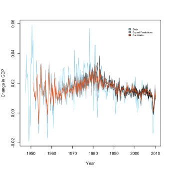
$a$ $b$

Figure 1: $a$: Quarterly growth rate of US GDP, 1948–2010, with predictions of the growing ensemble of AR(12) models and the weighted ensemble forecast. $b$ Accumulated regret of the ensemble, compared to combining global spline smoothing with an ARMA(8,7) model.

5 Discussion

5.1 Related Work

The closest approach to our method is that of Hazan and Seshadhri [7], who also work within the family of variants on multiplicative weight training. They introduce a new expert at each time step, whose initial weight is a fixed function of time, and do not otherwise implement a “fixed share” of weights, i.e., a minimum weight for each expert. Maintaining such a fixed share is extremely useful when a pre-existing model becomes one of the best, drastically cutting the time needed for it to dominate the ensemble. [7] also does not use tracking regret, but rather the maximum regret against any single expert attained over any contiguous time interval. This time-uniform regret is attractive, and they prove bounds on it, but only by assuming that each individual expert itself has a low, time-uniform regret (in the ordinary sense); some of their results even require low losses, not just low regrets. Our approach, by contrast, is able to accommodate the much more realistic situation where each individual expert may indeed have high loss, or even high regret, because the process is hard to predict and no one model is uniformly applicable.

Turning to more conventional approaches, econometrics has a large literature on detecting non-stationarity (of the basically-harmless “integrated” type characteristic of random walks), and finding “structural breaks” (change points), after which models must be re-estimated or re-specified [5]. Economists do not seem to have considered an ensemble method like ours, perhaps due to their laudable (if unfulfilled) ambition to capture the exact data-generating process in a single parsimonious model. Similarly, most work on data-set shift and concept drift in machine learning [15] deals with how a single model should be learned (or modified) so as to be robust to various changes in the joint distribution of inputs and outputs. Unlike all these approaches, we do not have to assume that any of our models are well-specified, nor assume anything about the nature of the data-generating process or how it changes over time.

There are some ensemble methods which are reminiscent of aspects of our proposal, such as Kolter and Maloof’s “additive expert ensemble” algorithm AddExp [11], the incremental-learning SEA algorithm [18], and adaptive time windows algorithms (e.g. [16]). None of these allow the full combination of a growing ensemble with temporally-specialized experts and adaptive weights. Consequently, while some of them can handle mild non-stationarities if the base models are close to well-specified, none of them are able to make strong individual-sequence prediction guarantees like those of Theorem 2.

5.2 Conclusion

We have introduced the growing-ensemble method, and shown that it leads to a modification of the conventional fixed-shares forecaster which is still Hannan-consistent, with $o(n)$ regret over $n$ time-steps compared to the retrospectively-best sequence of experts. This bound takes into account the fact that the ensemble grows continually and that individual experts can be arbitrarily bad, while the time series can have arbitrary non-stationarities. There are several interesting technical directions in which to take this (Can the counting of experts be replaced with variation of losses across the ensemble, as in [8]? Would it help to vary the weight with which new experts get introduced? Is there an optimal epoch length $\tau$?), the real importance of this work is methodological.

Complex systems tend to produce time series which are not just non-stationary but genuinely evolutionary — even if there is, in some sense, a fixed high-dimensional generative model, the dynamics of the low-dimensional variables we deal with changes in character over time. Tractable prediction models for such time series are at best local and transient approximations, no single one of which will work well for long. It is implausible even to come up with a fixed collection of models before we see how the system actually develops. Our growing ensemble method accommodates arbitrary dynamics, without assuming well-specified models, trends that can be extrapolated, stationary behavior punctuated by well-defined structural breaks, or other such props supporting previous work. Giving up the desire for the One True Model, of minimal risk, in favor of a growing ensemble of imperfect models, means we adapt automatically to arbitrary, historically evolving non-stationarities — including stationarity.

References

- [1] Paul Algoet. Universal schemes for prediction, gambling and portfolio selection. Annals of Probability, 20:901–941, 1992.
- [2] Sanjeev Arora, Elad Hazan, and Satyen Kale. The multiplicative weights update method: a meta algorithm and applications, 2005.
- [3] S. Caires and J. A. Ferreira. On the non-parametric prediction of conditionally stationary sequences. Statistical Inference for Stochastic Processes, 8:151–184, 2005. Correction, vol. 9 (2006), pp. 109–110.
- [4] Nicolò Cesa-Bianchi and Gábor Lugosi. Prediction, Learning, and Games. Cambridge University Press, Cambridge, England, 2006.
- [5] Michael P. Clements and David F. Hendry. Forecasting Non-stationary Economic Time Series. MIT Press, Cambridge, Massachusetts, 1999.
- [6] David N. DeJong and Chetan Dave. Structural Macroeconometrics. Princeton University PRess, Princeton, New Jersey, 2007.
- [7] Elad Hazan and C. Seshadhri. Efficient learning in algorithms for changing environments. In Proceedings of the 26th Annual International Conference on Machine Learning [ICML 2009], pages 393–400. ACM Press, 2009.
- [8] Elad Hazan and Satyen Kale. Extracting certainty from uncertainty: Regret bounded by variation in costs. Machine Learning, 80:165–188, 2010.
- [9] Mark Herbster and Manfred Warmuth. Tracking the best expert. Machine Learning, 32:151–178, 1998.
- [10] J. Zico Kolter and Marcus A. Maloof. Dynamic weighted majority: An ensemble method for drifting concepts. Journal of Machine Learning Research, 8:2755–2790, 2007.
- [11] Jeremy Z. Kolter and Marcus A. Maloof. Using additive expert ensembles to cope with concept drift. In Proceedings of the 22nd International Conference on Machine Learning, pages 449–456. ACM Press, 2005.
- [12] N. Littlestone and Manfred Warmuth. The weighted majority algorithm. Information and Computation, 108, 1994.
- [13] Donald S. Ornstein and Benjamin Weiss. How sampling reveals a process. Annals of Probability, 18:905–930, 1990.
- [14] Robert L. Paige and A. Alexandre Trindade. The Hodrick-Prescott filter: A special case of penalized spline smoothing. Electronic Journal of Statistics, 4:856–874, 2010.
- [15] Joaquin Quiñonero-Candela, Masashi Sugiyama, Anton Schwaighofer, and Neil D. Lawrence, editors. Dataset Shift in Machine Learning. MIT Press, Cambridge, Massachusetts, 2009.
- [16] Martin Scholz and Ralf Klinkenberg. An ensemble classifier for drifting concepts. In Porto ECML, editor, Proceedings of the Second International Workshop on Knowledge Discovery and Data Mining (KDD), 2005.
- [17] Robert H. Shumway and David S. Stoffer. Time Series Analysis and Its Applications. Springer Texts in Statistics. Springer-Verlag, New York, 2000.
- [18] W. N. Street and Y. Kim. A streaming ensemble algorithm (SEA) for large-scale classification. In Proceedings of the Second International Workshop on Knowledge Discovery and Data Mining (KDD), pages 377–382, New York, 2001. ACM Press.
- [19] Volodimir Vovk. Aggregating strategies. In Mark Fulk and John Case, editors, Proceedings of the Third Annual Workshop on Computational Learning Theory [COLT 1990], pages 371–386, San Francisco, 1990. Morgan Kaufmann.