Online Strategies for Intra and Inter Provider
Service Migration in Virtual Networks

Abstract

Network virtualization allows one to build dynamic distributed systems in which resources can be dynamically allocated at locations where they are most useful. In order to fully exploit the benefits of this new technology, protocols need to be devised which react efficiently to changes in the demand. This paper argues that the field of online algorithms and competitive analysis provides useful tools to deal with and reason about the uncertainty in the request dynamics, and to design algorithms with provable performance guarantees.

As a case study, we describe a system (e.g., a gaming application) where network virtualization is used to support thin client applications for mobile devices to improve their QoS. By decoupling the service from the underlying resource infrastructure, it can be migrated closer to the current client locations while taking into account migration cost. This paper identifies the major cost factors in such a system, and formalizes the corresponding optimization problem. Both randomized and deterministic, gravity center based online algorithms are presented which achieve a good tradeoff between improved QoS and migration cost in the worst-case, both for service migration within an infrastructure provider as well as for networks supporting cross-provider migration. The paper reports on our simulation results and also presents an explicit construction of an optimal offline algorithm which allows, e.g., to evaluate the competitive ratio empirically.

I Introduction

In 2008, the total number of mobile web users outgrew the total number of desktop computers with respect to Internet users [14] for the first time. Providing high quality-of-service (QoS) respective an excellent quality of experience (QoE) to mobile Internet clients is very challenging, e.g., due to user mobility. However, many applications, including such popular applications as gaming, need a reliable, continuous network service with minimal delay.

Network virtualization [12] is an emerging technology which allows a service specific network to be embedded onto a substrate network in a dynamic fashion. This includes migration of virtual nodes and links as well as virtual servers to meet the applications demands for connectivity and performance. To take full advantage of this flexibility it is often necessary to know future application demands. Yet, this information is typically not readily available and therefore neither the network resources can be used in an optimal manner nor do the users receive the best possible service.

This paper studies a mobile thin client application (such as a game server [20]) that is supported by network virtualization technology. We assume that the distribution of thin clients and therefore the request pattern changes over time. For instance, at 1 a.m. GMT many requests may originate in Asian countries, then more and more requests come from European users and later from the United States. In this setting it can be beneficial to migrate (or re-embed) the service closer to the users, e.g., to minimize access delays for the users and to minimize network costs for the providers [19]. Network virtualization allows us to realize such networks.

While moving services close to clients can reduce latency, migration also comes at a cost: the bulk-data transfer imposes load on the network and may cause a service disruption. In particular, the cost of migration depends on the available bandwidth in the substrate network [9]. Moreover, if virtual networks (VNets) are provisioned across administrative domains belonging to multiple infrastructure providers, (inter-provider) migration entails certain transit (or roaming) costs.

To gain insights into this tradeoff, we identify the main costs involved in this system. Intuitively, the benefits from virtualization are higher the lower the migration cost is relative to the latency penalty. Therefore, a predictable access pattern may ease migration. However, in practice, user arrival patterns are hard to predict, and thus we, in this paper, explicitly incorporate uncertainty about future arrivals.

The classic formal tool to study algorithms that deal with inputs (or more specifically: request accesses) that arrive in an online fashion and cannot be predicted is the competitive analysis framework. In competitive analysis, the performance of a so-called online algorithm is compared to an optimal offline algorithm that has complete knowledge of the input in advance. In effect, the competitive analysis is a worst case performance analysis that does not rely on any statistical assumptions. We apply this framework to network virtualization and propose—for a simplified model where, e.g., the main access cost is delay to the server and the main migration cost is the available bandwidth between migration source and destination—a competitive migration algorithm whose performance is close to the one of the optimal offline algorithm.

I-A Related Work

Mobile Networks. The mobile web today provides browser-based access to the Internet or web applications to millions of users connected to a wireless network via a mobile device. There exists a vast amount of work on the subject, and we refer the reader to the introductory books, e.g., [34]. In this project, we tackle the question of how network virtualization can be used to improve the quality of service for mobile devices.

Network Virtualization. Network virtualization has gained a lot of attention recently [35] as it enables the co-existence of innovation and reliability [31] and promises to overcome the “ossification” of the Internet [13]. For a more detailed survey on the subject, please refer to [12]. Virtualization allows to support a variety of network architectures and services over a shared substrate, that is, a Substrate Network Provider (SNP) provides a common substrate supporting a number of Diversified Virtual Networks (DVN). OpenFlow [25] and VINI [3] are two examples that allow researchers to (simultaneously) evaluate protocols in a controllable and realistic environment. Trellis [4] provides a software platform for hosting multiple virtual networks on shared commodity hardware and can be used for VINI. Network virtualization is also useful in data center architectures, see, e.g., [18].

Embedding. A major challenge in network virtualization is the embedding [26] of VNets, that is, the question of how to efficiently and on-demand assign incoming service requests onto the topology. Due to its relevance, the embedding problem has been intensively studied in various settings, e.g., for an offline version of the embedding problem see [23], for an online and competitive algorithm see [15], for an embedding with only bandwidth constraints see [16], for heuristic approaches without admission control see [38], or for a simulated annealing approach see [29]. Since the general embedding problem is computationally hard, Yu et al. [24] advocate to rethink the design of the substrate network to simplify the embedding; for instance, they allow to split a virtual link over multiple paths and perform periodic path migrations. Lischka and Karl [22] present an embedding heuristic that uses backtracking and aims at embedding nodes and links concurrently for improved resource utilization. Such a concurrent mapping approach is also proposed in [10] with the help of a mixed integer program (a more general formulation which also includes migration aspects can be found in [30]). Finally, several challenges of embeddings in wireless networks have been identified by Park and Kim [27].

In contrast to the approaches discussed above we, in this paper, tackle the question of how to dynamically embed or migrate virtual servers [28] in order to efficiently satisfy connection requests arriving online at any of the network entry points, and thus use virtualization technology to improve the quality of service for mobile nodes. The relevance of this subproblem of the general embedding problem is underlined by Hao et al. [19] who show that under certain circumstances, migration of a Samba front-end server closer to the clients can be beneficial even for bulk-data applications.

Online Algorithms. To the best of our knowledge, [5] and [1] (for online server migration), and [15] (for online virtual network embeddings) are the only works to study network virtualization from an online algorithm perspective. The formal competitive migration problem is related to several classic optimization problems such as facility location, $k$-server problems, or online page migration. All these problems are a special case of the general metrical task system (e.g., [7, 8]) for which there is, e.g., an asymptotically optimal deterministic $\Theta(n)$-competitive algorithm, where $n$ is the state (or “configuration”) space; or a randomized $O(\log^{2}n\cdot\log\log{n})$-competitive algorithm given that the state space fulfills the triangle inequality: this algorithm uses a (well separated) tree approximation for the general metric space (in a preprocessing step) and subsequently solves the problem on this distorted space; unfortunately, both algorithmic parts are rather complex.

In the field of facility location, researchers aim at computing optimal facility locations that minimize building costs and access costs (see, e.g., [17] for an online algorithm). In [21], Laoutaris et al. propose a heuristic algorithm for a variant of a facility location problem which allows for facility migration; this algorithm uses neighborhood-limited topology and demand information to compute optimal facility locations in a distributed manner. In contrast to our work, the setting is different and migration cost is measured in terms of hop count. There is no performance guarantee. In the field of $k$-server problems (e.g., [7]), an online algorithm must control the movement of a set of $k$ servers, represented as points in a metric space, and handle requests that are also in the form of points in the space. As each request arrives, the algorithm must determine which server to move to the requested point. The goal of the algorithm is to reduce the total distance that all servers traverse. In contrast, in our model it is possible to access the server remotely, that is, there is no need for the server to move to the request’s position. The page migration problem (e.g., [2]) occurs in managing a globally addressed shared memory in a multiprocessor system. Each physical page of memory is located at a given processor, and memory references to that page by other processors are charged a cost equal to the network distance. At times, the page may migrate between processors, at a cost equal to the distance times a page size factor. The problem is to schedule movements on-line so as to minimize the total cost of memory references. In contrast to these page migration models, we differentiate between access costs that are determined by latency and migration costs that are determined by network bandwidth.

There is an intriguing relationship between server migration and online function tracking [6, 36]. In online function tracking, an entity Alice needs to keep an entity Bob (approximately) informed about a dynamically changing function, without sending too many updates. The online function tracking problem can be transformed into a chain network where the function values are represented by the nodes on the chain, and a sequence of value changes corresponds to a request pattern on the chain. In particular, it follows from [6] that already for some very simple linear substrate networks of size $n=\Theta(\beta)$, where $\beta$ is the migration cost, no deterministic or randomized online algorithm can achieve a competitive ratio smaller than $\Omega(\log n/\log\log n)$.

Other. A preliminary version of this paper was presented at the VISA workshop [5] (a discussion of multiple server scenarios appeared at the Hot-ICE workshop [1]). We extend the results in [5] in several respects: First, we present a deterministic alternative to the randomized migration strategy derived in [5]; this deterministic online algorithm is based on gravity centers and achieves a better competitive ratio against adaptive adversaries. Second, we extend our model to settings with multiple infrastructure providers, and describe competitive intra and inter provider migration strategies. Provisioning virtual network services across multiple providers is an interesting topic which is hardly explored in literature so far; notable exceptions are PolyVINE [11], a distributed coordination protocol to perform cross-provider embeddings, and V-Mart [37] that describes an auction framework for task partitioning. Third, we conducted extensive experiments to complement our formal analysis.

I-B Contributions and Organization

This paper studies a mobile network virtualization architecture where thin clients on mobile devices access a service that can be migrated closer to the access points to reduce user latency. We identify the main costs in this system (Section II) and introduce an optimization problem accordingly. Both for networks with a single provider (Section III) as well as for networks with multiple providers (Section IV), online migration strategies are presented that are provably competitive to an optimal offline algorithm, i.e., that achieve a good performance even in the worst-case. This paper also describes an optimal offline algorithm which is useful for finding optimal strategies at hindsight, for dealing with regular and periodic request patterns, and for computing the competitive ratios of online algorithms (Section V). We report on our experiments in different scenarios in Section  VI. In Section VII, the paper concludes.

II Architecture

Our work is motivated by the virtualization architecture proposed in [31] for which we are in the process of developing a prototype implementation. The main roles of this architecture related to this work are: The (Physical) Infrastructure Provider (PIP), which owns and manages an underlaying physical infrastructure called “substrate” (we will treat the terms infrastructure provider and substrate provider as synonyms); the Virtual Network Provider (VNP), which provides bit-pipes and end-to-end connectivity to end-users; and the Service Provider (SP), which offers application, data and content services to end-users.

We assume that a service provider is offering a service to mobile clients which can benefit from the flexibility of network and service virtualization. The goal of the service provider is to minimize the round-trip-time of its service users to the servers, by triggering migrations depending, e.g., on (latency) measurements. Concretely, VNP and/or PIPs will react on the SP-side changes of the requirements on the paths between server and access points, and re-embed the servers accordingly.

In the remainder of this paper, if not stated otherwise, the term provider will refer to the PIP role in the above architecture. In particular, we will study multi provider scenarios where the service provider may decide to migrate an application across PIP boundaries.

II-A General Cost Model

Formally, we consider a substrate network $G=(V,E)$ managed by one or multiple substrate providers (PIP). Each substrate node $v\in V$ has certain properties and features associated with it (e.g., in terms of operating system or CPU power); in particular, we assume that it has a computational capacity $c(v)$. Similarly, each link $e=(u,v)\in E$, with $u,v\in V$, has certain properties, e.g., it is characterized by a bandwidth capacity $\omega(e)$, and it offers the latency $\lambda(e)$. Links between different PIPs are typically more expensive than links within a PIP.

In addition to the substrate network, there is a set $T$ of external machines (the mobile thin clients or simply terminals) that access $G$ by issuing requests to virtualized services hosted on a set of virtual servers by $G$. There is a set of services $\mathcal{S}=\{S_{1},S_{2},...\}$ where each service $S_{i}$ can be offered by multiple servers $s\in S_{i}$. (In the technical part of the paper we will focus on a single-server scenario only.) Each server $s$ has a certain resource or capacity requirement $r(s)$ that needs to be allocated to $s$ on the substrate node where it is hosted.

In order for the machines in $T$ to access the services $\mathcal{S}$, a fixed subset of nodes $A\subseteq V$ serve as Access Points where machines in $T$ can connect to $G$. Due to the movement of machines in $T$, the access points can change frequently, which may trigger the migration algorithm. We define $\sigma_{t}$ to be the multi-set of requests at time $t$ where each element is a tuple $(a\in A,S\in\mathcal{S})$ specifying the access point and the requested service $S$. (For ease of notation, when clear from the context, we will sometimes simply write $v\in\sigma_{t}$ to denote the multi-set of access points used by the different requests.) Our main objective is to shed light onto the trade-off between the access costs $\text{Cost}_{\text{acc}}$ of the mobile clients to the current service locations and the server migration cost $\text{Cost}_{\text{mig}}$: while moving the servers closer to the requester may reduce the access costs and hence improve the quality of service, it also entails the overhead of migration.

We can identify the following main parameters which influence the access and migration costs. A major share of $\text{Cost}_{\text{acc}}$ is due to the request latency, i.e., the sum of the requests’ latencies to the corresponding servers. Observe that the routing of the requests occurs along the shortest paths (w.r.t. latency) on the substrate network. In addition, the access cost depends on the server load, that is, the access cost depends on the capacity $c(v)$ of the hosting node $v$ and the resource demands $r(s)$ of the servers $s$ hosted by $v$. The correlation between load and delay can be captured by different functions, and is not studied further here. In this paper, we assume that requests are relatively small, and hence, we do not explicitly model bandwidth constraints in $\text{Cost}_{\text{acc}}$. In conclusion, at time $t$ and for some function $f$,

$$\text{Cost}_{\text{acc}}(t)=\sum_{r_{t}\in\sigma_{t}}f\left(\text{delay}(r_{t}),\text{load}(r_{t})\right).$$

In contrast to the requests, which are rather light-weight, the server state is typically large, and hence the traffic volume of migration cannot be neglected. The main cost of migration are service outage periods and the migration itself. The migration cost $\text{Cost}_{\text{mig}}$ of a virtual server $s\in S$, or the outage period, hence depends to a large extent on the available bandwidth $\omega(p)$ on the migration path $p:src\rightsquigarrow dst$ (along the substrate network) between migration source node $src$ and destination node $dst$, and the size $\text{size}(s)$ of the application $s$ to be migrated. Another major cost factor is the transit costs, namely the number $k$ of PIPs on the path. In summary:

$$\text{Cost}_{\text{mig}}(t)=\sum_{s\in S}f(\omega(p),k,\text{size}(s))$$

for some function $f$, where the migration cost is zero if $src=dst$.

Our model so far lacks one additional ingredient: terminal dynamics (or mobility). One approach would be to assume arbitrary request sets $\sigma_{t}$, where $\sigma_{t}$ is completely independent of $\sigma_{t-1}$. However, for certain applications it may be more realistic to assume that the mobile nodes move “slowly” between the access points. Note that while users typically travel between different cities or countries at a limited speed, these geographical movements may not translate to the topology of the substrate network. Thus, rather than modeling the users to travel along the links of $G$, we consider on/off models where a user appears at some access point $a_{1}\in A$ at time $t$, remains there for a certain period $\Delta t$, before moving to another arbitrary node $a_{2}\in A$ at time $t+\Delta t$.

One may assume that $\Delta t$ is exponentially distributed. However, in our formal analysis we assume a worst-case perspective and consider arbitrary distributions for $\Delta t$. Often, it is reasonable to assume some form of correlation between the individual terminals’ movement. For example, in an urban area, workers commute downtown in the morning and return to suburbs in the evening. Or in a planetary-scale substrate network, demographic aspects have to be taken into account in the sense that during a day, first many requests will originate from Asian countries, followed by an active period in Europe and finally America. However, as it is rather hard to describe and characterize such movement accurately we, in the formal part of this paper, perform a worst case analysis (w.r.t. latency) that does not use any statistical assumptions.

To what extent the system can benefit from virtual network support and migration depends on several factors, e.g., how frequently the thin clients change the access points. Given rapid changes it may be best to place the server in the middle of the network and leave it there. On the other hand, if the changes are slower or can be predicted, it can be worthwhile to migrate the server to follow the mobility pattern. This constitutes the trade-off studied in this paper.

II-B Competitive Analysis

As already discussed, competitive analysis asks the question: How well does the system perform compared to an optimal offline strategy which has complete knowledge of the entire request sequence in advance? In the following, we present an online migration strategy that is “competitive” to any other online or offline solution for virtual network supported server migration. In order to focus on the main properties and trade-offs involved in the virtualization support of thin clients, we assume a simplified online framework for our formal analysis. We consider a synchronized setting where time proceeds in time slots (or rounds). In each round $t$, a set of $\sigma_{t}$ terminal requests arrive in a worst-case and online fashion at an arbitrary set of access nodes $A$.

Thus the embedding problem is equivalent to the following synchronous game, where an online algorithm Alg has to decide on the migration strategy in each round $t$, without knowing about the future access requests. In each round $t\geq 0$:

1. The requests $\sigma_{t}$ arrive at some access nodes $A$.

2. The online algorithm Alg decides where in $G$ to migrate the servers $S$. If positions are changed, it pays migration costs $\text{Cost}_{\text{mig}}(t)$.

3. The online algorithm Alg pays the requests’ access costs $\text{Cost}_{\text{acc}}(t)$ to the corresponding servers (e.g, hop distance).

Note, that we allow Alg to migrate the virtual servers for all the requests of the current time slot $t$. However, as we assume that a request is much cheaper than a migration, and if there are not too many requests arriving concurrently, our results also apply to scenarios where the last two steps are reordered.

We aim at devising competitive algorithms Alg that minimize the competitive ratio $\rho$: Let $\textsc{Alg}_{t}(\sigma)$ be the migration and access costs incurred by Alg in round $t$ under a request arrival sequence $\sigma$ (a sequence of access points), that is,

$$\textsc{Alg}_{t}(\sigma)=\text{Cost}_{\text{acc}}(t)+\text{Cost}_{\text{mig}}(t).$$

Let $\textsc{Opt}(\sigma)$ be the optimal cost of an offline algorithm Opt for the given $\sigma$, that is, Opt has a complete knowledge of $\sigma$ and can hence optimize the server locations “offline”. $\rho$ is the ratio of the costs of Alg and Opt. Thus, our objective is to minimize:

$$\rho=\max_{\sigma}\frac{\sum_{t}\textsc{Alg}_{t}(\sigma)}{\textsc{Opt}(\sigma)}$$

In case of online algorithms that use randomization, we consider the expected costs against an oblivious adversary without access to the outcome of the random coin flips of the algorithm.

For our analysis, we make the following simplification: The migration cost $\text{Cost}_{\text{mig}}(t)$ is given by the bandwidth constraint of the smallest edge capacity on the migration path, plus the number of PIPs traversed times $\pi$. Let $\text{Cost}_{\text{mig}}(u,v)$ denote the migration cost on a path from $u$ to $v$. (The path will be clear from the context.) Thus, $\text{Cost}_{\text{mig}}(u,v)=\max_{e}\text{size}(s)/\omega(e)+k\cdot\pi$ where $\text{size}(s)$ is the size of the migrated server $s$, $e$ is a link on the migration path from $u$ to $v$, $k$ is the number of PIPs traversed and $\pi$ is the cost of migrating across a PIP boundary. Observe that given a migration path, the cost is different in case the migration occurs once along the entire path compared to the case where it occurs in two steps at different times.

III Competitive Intra-Provider Migration

This section presents two online protocols for server migration within a single provider (PIP). The main idea of both algorithms is to divide time into epochs: As we will see, also an optimal offline algorithm will have certain costs in such an epoch, which allows us to compare its performance to the online algorithms. While algorithm Mix uses randomization to identify good locations to serve the current requests, algorithm Cen deterministically migrates to the gravity centers of the demand. Before describing these two algorithms in detail, we briefly discuss static strategies without migration.

III-A The Stat Algorithm

In order to compare the benefits of migration to a static scenario, we derive the competitive ratio of fixed strategies (see also [5]).

Lemma III.1

A system without migration yields a competitive ratio of

$$\rho\in\Theta(\text{Diam}(G)),$$

where $\text{Diam}(G)$ is the network diameter of substrate network $G$. [5]

In a fixed scenario, the best static algorithm Stat hosts $s$ is in the network center, i.e., the location which minimizes the worst-case distance traveled by the requests, namely at node $u$ for which $u:=\arg\min_{v\in V}\max_{w\in V}\text{Cost}_{\text{acc}}(v,w).$

Note, since there is no migration in the fixed scenario, the competitive ratio does not depend on any bandwidth constraints (i.e., on link weights). This means that in networks with highly heterogeneous links or with links whose capacity changes quickly over time, a static solution without migration may be good.

III-B The Mix Algorithm

We now describe an online migration algorithm Mix (see also [5]). The basic idea of Mix is to strike a balance between the request latency cost $\text{Cost}_{\text{acc}}^{\textsc{Mix}}$ and the migration cost $\text{Cost}_{\text{mig}}^{\textsc{Mix}}$ it incurs, and to continuously move closer to a possible optimal position. The intuition is that after a small number of migrations only, either Mix is at the optimal position, or an optimal offline algorithm Opt must have migrated as well during this time period. Either way, Opt cannot incur much smaller costs than Mix. In other words, by using Mix for moving to good locations in the network, a possible offline algorithm that migrates less frequently cannot have much lower access costs than Mix; on the other hand, an offline strategy with frequent migrations will have similar costs to $\text{Cost}_{\text{mig}}$.

Let us first consider a scenario with constant bandwidth capacities, i.e., $\omega(e)=\omega~{}~{}\forall e\in E$ and let $\beta=\text{size}(s)/\omega$ be the corresponding migration cost.

The algorithm Mix divides time into epochs. In each epoch Mix monitors, for each node $v$, the cost of serving all requests from this epoch by a server kept at $v$. We denote this counter by $\textsc{C}(v)$. Mix keeps the server at a single node $w$ till $\textsc{C}(w)$ reaches $\beta$. In this case, Mix migrates the server to a node $u$ chosen uniformly at random among nodes with the property $\textsc{C}(u)<\beta$. If there is no such node, Mix does not migrate the server, and the epoch ends in that round; the next epoch starts in the next round and the counters $\textsc{C}(v)$ are reset to zero.

Lemma III.2

Mix is $O(\log n)$-competitive in networks with constant bandwidth. [5]

Proof:

Fix any epoch $\mathcal{E}$ and let $\beta$ denote the migration cost. If Opt migrates the server within $\mathcal{E}$, it pays $\beta$. Otherwise it keeps it at a single node paying the value of the corresponding counter at the end of $\mathcal{E}$. By the construction of Mix, this value is at least $\beta$, and thus in either case $\textsc{Opt}(\mathcal{E})\geq\beta$.

The migrations performed by Mix partition $\mathcal{E}$ into several phases. According to our migration strategy, the access cost of Mix in each phase is at most $\beta$. In [5], we show that the expected number of migrations within one epoch is at most $H_{n}$, where $H_{n}$ is the $n$-th harmonic number. The number of phases is then $H_{n}+1$, and hence $\textsc{Mix}(\mathcal{E})\leq\beta\cdot H_{n}+\beta\cdot(H_{n}+1)=\beta\cdot O(\log n)$. This yields the competitiveness of Mix. ∎

Note that the analysis does not rely on access costs being measured as the number of hops. Rather, the analysis (and hence also the result) is applicable to any metric which ensures that counters increase monotonically over time, i.e., with additional requests.

For networks with general bandwidths, Mix can be adopted in such a way that it migrates when the counter of the current location $v$ reaches $\text{size}(s)/\min_{e}\omega(e)$, that is, when $\textsc{C}(v)\geq\text{size}(s)/\min_{e}\omega(e)$. Thus, the cost of the optimal algorithm in each epoch is at least $\text{size}(s)/\max_{e}\omega(e)$, while the cost of Mix is at most $\text{size}(s)/\min_{e}\omega(e)$. Therefore, by the same arguments as in the proof of Lemma III.2, we immediately obtain the following result.

Theorem III.3

Mix is $O(\mu\cdot\log n)$-competitive in general networks, where $\mu=\max_{e,e^{\prime}\in E}\omega(e)/\omega(e^{\prime})$.

III-C The Cen Algorithm

While for the analysis of Mix, we assumed an oblivious adversary which cannot be adaptive with respect to the random choices made by the online algorithm, we now focus on deterministic algorithms Cen. As we will see, a logarithmic competitive ratio can also be achieved. Again, we will first assume $\omega(e)=\omega~{}~{}\forall e\in E$ and $\beta=\text{size}(s)/\omega$.

Cen divides time into epochs consisting of one or multiple phases between which Cen migrates. Again, we have counters $\textsc{C}(v)$ for each node $v$ that are set to zero at the beginning of an epoch. These counters accumulate the access costs of an epoch if the server was permanently located at $v$. Henceforth, we will call all nodes $v$ for which at time $t$, $\textsc{C}(v)<\beta/40$, active nodes at time $t$. Assume that algorithm Cen is currently at some node $v$. Cen remains at this node until it accumulated there access costs of $\beta$. Then, a new phase starts, and Cen computes the gravity center $w$, i.e., the “center” of the currently active nodes. Formally, let $d$ denote the shortest path metric (w.r.t. access costs) on the network $G$. The gravity center of a subset $V^{\prime}\subseteq V$ of nodes is defined as the (not necessarily unique) node $\mathcal{G}(V^{\prime})=\arg\min_{v\in V^{\prime}}\sum_{u\in A}d(u,v)$, where $A$ is the set of access points. (Ties are broken arbitrarily.) Cen migrates to $w$ and a new phase starts. If there is no active node left, the epoch ends.

In order to study the competitive ratio of Cen, we exploit the fact that a request always increases the counter of several nodes besides the gravity center (namely: a constant fraction) by at least a certain value (again, a constant fraction) as well.

Lemma III.4

Let $\lambda_{1}=1/5$ and $\lambda_{2}=1/4$. Fix any active set $V^{\prime}$. Let $r$ be an arbitrary requesting node (at some step). Assume the counter at the gravity center $\mathcal{G}(V^{\prime})$ increased by $F$ because of this request. Then there are at least $\lambda_{2}\cdot|V^{\prime}|$ nodes from $V^{\prime}$ whose counters increased at least by $\lambda_{1}\cdot F$.

Proof:

Assume the contrary. It means that there are at least $(1-\lambda_{2})\cdot|V^{\prime}|$ nodes from $V^{\prime}$ whose counter increase is smaller than $\lambda_{1}\cdot F$. Denote this set by $V^{\prime\prime}$. We know that the distance between the request and the center is $d(\mathcal{G}(V^{\prime}),r)=F$, and $\forall u\in V^{\prime\prime}$, $d(u,r)<\lambda_{1}\cdot F$. Therefore, $\forall u,v\in V^{\prime\prime}$, $d(u,v)<2\lambda_{1}\cdot F$: the diameter of the set $V^{\prime\prime}$ is relatively small.

Now let $\xi$ be any node of $V^{\prime\prime}$. We show that $\xi$ would be a better candidate for the gravity center than $\mathcal{G}(V^{\prime})$ is. Using triangle inequalities, we obtain

$$\sum_{u\in V^{\prime}}d(\mathcal{G}(V^{\prime}),u)\;= \;\sum_{u\in V^{\prime\prime}}d(\mathcal{G}(V^{\prime}),u)+\sum_{u\in V^{\prime}\setminus V^{\prime\prime}}d(\mathcal{G}(V^{\prime}),u)$$

$$\geq \;\sum_{u\in V^{\prime\prime}}\left[d(\mathcal{G}(V^{\prime}),r)-d(u,r)\right]$$

$$+\sum_{u\in{V^{\prime}\setminus V^{\prime\prime}}}d(\mathcal{G}(V^{\prime}),u)$$

$$> \;(1-\lambda_{1})\cdot|V^{\prime\prime}|\cdot F+\sum_{u\in{V^{\prime}\setminus V^{\prime\prime}}}d(\mathcal{G}(V^{\prime}),u)$$

$$> \;\frac{4}{5}\cdot|V^{\prime\prime}|\cdot F+\sum_{u\in V^{\prime}\setminus V^{\prime\prime}}d(\mathcal{G}(V^{\prime}),u)\enspace$$

because $d(\mathcal{G}(V^{\prime}),r)=F$ and $d(u,r)\leq\lambda_{1}\cdot F$, and by substituting $\lambda_{1}=1/5$. On the other hand, note that $|V^{\prime}\setminus V^{\prime\prime}|\leq|V^{\prime}|/4\leq|V^{\prime\prime}|/3$ and

$$\sum_{u\in V^{\prime}}d(\xi,u)\;= \;\sum_{u\in V^{\prime\prime}}d(\xi,u)+\sum_{u\in V^{\prime}\setminus V^{\prime\prime}}d(\xi,u)$$

$$< \;2\lambda_{1}\cdot|V^{\prime\prime}|\cdot F$$

$$+\sum_{u\in V^{\prime}\setminus V^{\prime\prime}}\left[d(\xi,r)+d(r,\mathcal{G}(V^{\prime}))+d(\mathcal{G}(V^{\prime}),u)\right]$$

$$< \;2\lambda_{1}\cdot|V^{\prime\prime}|\cdot F+|V^{\prime}\setminus V^{\prime\prime}|\cdot(1+\lambda_{1})\cdot F$$

$$+\sum_{u\in V^{\prime}\setminus V^{\prime\prime}}d(\mathcal{G}(V^{\prime}),u)$$

$$\leq \;\frac{4}{5}\cdot|V^{\prime\prime}|\cdot F+\sum_{u\in V^{\prime}\setminus V^{\prime\prime}}d(\mathcal{G}(V^{\prime}),u)\enspace$$

because $d(\xi,r)<\lambda_{1}\cdot F$, $d(r,\mathcal{G}(V^{\prime}))=F$, and by substituting the value of $\lambda_{1}=1/5$. This contradicts that $\mathcal{G}(V^{\prime})$ is the gravity center of $V^{\prime}$. ∎

From Lemma III.4 it follows that when the counter at the gravity center exceeds a given threshold, the counter of many nodes besides the center must be high as well.

Lemma III.5

Fix any threshold $\tau$. When the counter at the gravity center $\mathcal{G}(V^{\prime})$ exceeds $\tau$, then there exists $V^{\prime\prime}\subseteq V^{\prime}$, $|V^{\prime\prime}|\geq\frac{1}{8}\cdot|V^{\prime}|$, such that for all $v\in V^{\prime\prime}$, the counter at $v$ is at least $\tau/40$.

Proof:

Assume the contrary. This means that there exists $V^{\prime\prime}\subseteq V^{\prime}$, $|V^{\prime\prime}|\geq\frac{7}{8}\cdot|V^{\prime}|$, such that for all $v\in V^{\prime\prime}$, the counter at $v$ is smaller than $\tau/40$. Hence $\sum_{v\in V^{\prime\prime}}\textsc{C}(v)<|V^{\prime\prime}|\cdot\tau/40\leq|V^{\prime}|\cdot\tau/40$. On the other hand, by Lemma III.4, each time the counter $\textsc{C}(\mathcal{G}(V^{\prime}))$ increases by $F$, at least $1/4\cdot|V^{\prime}|$ counters from set $V^{\prime}$ (and hence at least $1/8\cdot|V^{\prime}|$ counters from set $V^{\prime\prime}$, since $|V^{\prime}\setminus V^{\prime\prime}|\leq\frac{|V^{\prime}|}{8}$) increase by $F/5$. Hence, in this case, the sum of counters from $V^{\prime\prime}$ increases at least by $1/40\cdot|V^{\prime}|\cdot F$. Therefore, when $\textsc{C}(\mathcal{G}(V^{\prime}))\geq\tau$, $\sum_{v\in V^{\prime\prime}}\textsc{C}(v)\geq|V^{\prime}|\cdot\tau/40$, which is a contradiction. ∎

For the competitive ratio, we therefore have the following result.

Theorem III.6

Cen is $O(\log{n})$-competitive.

Proof:

First, we consider the cost of the optimal offline algorithm. If Opt migrates in an epoch, it has costs $\beta$. Otherwise, due to the definition of Cen, as there are no active nodes left at the end of an epoch, the access costs of any node is also in the order of $\Omega(\beta)$. Regarding Cen, we know that in each phase, access costs are at most $\beta$, and it remains to study the number of phases per epoch. By Lemma III.5, we know that in each phase, the number of active nodes is reduced by a factor at least $1/8$. Therefore, there are at most $O(\log{n})$ many phases per epoch, and the claim follows. ∎

Note that we did not try to optimize the constants in this proof, and in practice (and in our simulations), alternative thresholds can be applied yielding better (but qualitatively equivalent) results.

Again, for networks with general bandwidths, Cen can be adopted in such a way that it migrates when the counter of the current location $v$ reaches $\text{size}(s)/\min_{e}\omega(e)$, that is, when $\textsc{C}(v)\geq\text{size}(s)/\min_{e}\omega(e)$. By the same arguments as above, this adds a factor $\max_{e,e^{\prime}\in E}\omega(e)/\omega(e^{\prime})$ to the competitive ratio.

III-D Remarks

Recall that the adversarial model for Mix and Cen is different, and hence, one has to be careful when comparing the competitive ratios: the bound for Mix only holds against oblivious adversaries, and we expect the center of gravity approach to perform better in worst-case scenarios with adaptive adversaries. Our simulations show that the question which of the two strategies is more efficient depends on the scenario.

Also note that both Mix and Cen are quite general with respect to the measure of access costs, i.e., the derived bounds hold for arbitrary latency functions on the links in case of Mix. This allows us to generalize our analysis to scenarios where the access latency, in addition to the sum of the link latencies, depends also on the capacity of the hosting node: We simply need to take the capacities into account when increasing the counters. In case of Cen, the access costs must fulfill the triangle inequality.

IV Inter-Provider Migration

The flexibility offered by network virtualization is not limited to a single PIP. Rather, a Virtual Network Provider may have contracts with multiple infrastructure providers, and provision a service across PIP boundaries. In the following, we extend our model to multiple provider scenarios. In particular, we assume that migrating a server across a PIP boundary entails a fixed “roaming” cost $\pi$ for each transit. Since we assume that a PIP typically does not reveal its internal resource structure, we seek to come up with migration algorithms that pose minimal requirements on the knowledge of a PIP topology.

In order to study the benefits of migration, we again consider a scenario without migration (algorithm Stat). Of course, Lemma III.1 still applies: in a fixed scenario, the best location for hosting $s$ is in the network center, i.e., the location which minimizes the distance traveled by the requests.

In the following, we present how the randomized algorithm Mix and the deterministic algorithm Cen can be extended to multi-PIP scenarios. We consider $k$ PIPs, migration inside a PIP costs $\beta$, access costs are the number of hops, and migrating across providers costs $\pi$ per crossed PIP boundary. We will concentrate on the more realistic case where $\pi\geq\beta$. (If $\pi<\beta$, our single PIP algorithms could be applied without taking into account transit costs. This yields a performance in the order as derived for the case $\pi\geq\beta$.)

It is sometimes useful to think of the PIP graph, the graph where all the nodes of one PIP form one vertex and two PIPs are connected if there is a connection between nodes of the respective PIPs in the substrate graph. In particular, we will refer to the diameter of the PIP graph, the largest number of PIPs to be traversed on a shortest migration path, by $\Delta$.

Algorithm $\textsc{Mix}_{k}$ generalizes Mix by moving the server to one of the PIPs having lower costs.

The algorithm $\textsc{Mix}_{k}$ divides time into three types of epochs: huge epochs which consist of one or several large epochs which in turn consist of $\lceil\pi/\beta\rceil$ small epochs. For each node $u$, we use two counters $\textsc{C}(u)$ and C_L($u$) to count the access cost during a small and a large epoch, respectively. At the beginning of a small epoch, all nodes are active; similarly, at the beginning of a huge epoch, we say that all PIPs are active. During a small epoch, the server is migrated within a single PIP only, until there is no node $u$ left with access costs smaller than $\beta$: $\textsc{Mix}_{k}$ monitors, for each node $u$, the cost of serving all requests from this small epoch by a server kept at $u$; $\textsc{Mix}_{k}$ keeps the server at a single node $u$ till $\textsc{C}(u)$ reaches $\beta$. When this happens, $\textsc{Mix}_{k}$ migrates the server to a node $v$ chosen uniformly at random among nodes of the current PIP with the property $\textsc{C}(v)<\beta$. If there is no such node, $\textsc{Mix}_{k}$ does not migrate the server, and the small epoch ends in that round; the next epoch starts in the next round and the counters $\textsc{C}(u)$ are reset to zero.

After $\lceil\pi/\beta\rceil$ small epochs a large epoch ends. Then $\textsc{Mix}_{k}$ determines the set of PIPs that contain at least one node $v$ for which C_L($v$)$<\pi$; all other PIPs become inactive for the remainder of the current huge epoch. If there are active PIPs left, $\textsc{Mix}_{k}$ chooses an active PIP uniformly at random and migrates to an arbitrary node of that PIP; otherwise the server stays where it is, and a new huge epoch begins.

We can derive the following competitive ratio on $\textsc{Mix}_{k}$’s performance.

Theorem IV.1

$\textsc{Mix}_{k}$ is $O(\log{k}\cdot(\log{n_{1}}+\Delta))$-competitive in networks with constant bandwidth and $k$ PIPs, where $n_{1}$ is the size of the largest PIP, and $\Delta$ is the “diameter of the PIP graph”.

Proof:

From Lemma III.2, we know that during a small epoch, $\textsc{Mix}_{k}$ accumulates a cost of at most $O(\beta\log{n_{1}})$: There is at most a logarithmic number of migrations, and the access costs per phase is at most $\beta$. Recall that a large epoch consists of at most $\lceil\pi/\beta\rceil$ many small epochs, and subsequently, a remaining active PIP is chosen uniformly at random. Thus, similarly to Lemma III.2, it holds that there are at most $O(\log k)$ many large epochs, yielding a total access cost of $O(\log{k}\cdot\log{n_{1}}\cdot\pi/\beta\cdot\beta)=O(\pi\log k\cdot\log n)$. The migration costs within PIPs are of the same order. The transit costs to move the server between PIPs amounts to at most $O(\Delta\pi\log{k})$. Thus, the overall cost of $\textsc{Mix}_{k}$ per huge epoch is in the order of $O(\pi\log{k}\cdot(\log{n_{1}}+\Delta))$. On the other hand, an optimal offline algorithm must have had costs of at least $\pi$ as well during this huge epoch: if the optimal algorithm migrates between PIPs, the claim follows trivially. Otherwise, the optimal offline algorithm is located at a single PIP during the entire huge epoch; by the construction of $\textsc{Mix}_{k}$, there must exist a large epoch in which the optimal offline algorithm incurred a cost of at least $\Omega(\pi)$: per small epoch the (access or migration) costs are at least $\beta$, and there are $\lceil\pi/\beta\rceil$ many small epochs in a large epoch. The claim follows. ∎

Note that the proof of Theorem IV.1 is overly pessimistic, as it assumes several large migration distances that the optimal offline algorithm can avoid. We believe that $\textsc{Mix}_{k}$ performs better, also in the worst-case, a conjecture that is also manifested by our experiments.

A similar extension also works for the deterministic variant.

The algorithm $\textsc{Cen}_{k}$ divides time into three types of epochs: a huge epoch consists of multiple large epochs, and a large epoch consists of $40\lceil\pi/\beta\rceil$ small epochs. Again, we use counters $\textsc{C}(u)$ to accumulate the access costs of a node $u$ during a small epoch; in addition, a counter C_L($u$) is used to accumulate access costs during a large epoch. In the beginning, all PIPs are set to active. At the beginning of a small epoch, the $\textsc{C}(u)$ values are set to zero for all nodes within the current PIP. $\textsc{Cen}_{k}$ then monitors, for each node $u$, the cost of serving all requests from this small epoch by a server kept at $u$. $\textsc{Cen}_{k}$ leaves the server at a single node $u$ till $\textsc{C}(u)$ reaches $\beta$. In this case, $\textsc{Cen}_{k}$ migrates the server to a node $v$ which constitutes the center of gravity among the active nodes of the current PIP, i.e., the nodes $w$ of the current PIP for which it still holds that $\textsc{C}(w)<\beta/40$. If there is no active node left within the current PIP, a small epoch ends in that round; the next small epoch starts in the next round. After $40\lceil\pi/\beta\rceil$ small epochs, a new large epoch starts, and all nodes $u$ in the network with C_L($u$)$\geq\pi/40$ become inactive with respect to the large epoch. Among all remaining active nodes of the large epoch, $\textsc{Cen}_{k}$ determines the center of gravity of all nodes and moves the server to the corresponding PIP, and a new large epoch begins. Otherwise, if there is no PIP left that contains active nodes, the server stays where it is, and a new huge epoch starts.

We can show the following result.

Theorem IV.2

$\textsc{Cen}_{k}$ is $O(\log{n}(\log{n_{1}}+\Delta))$-competitive in networks with constant bandwidth and $k$ PIPs, where $n_{1}$ is the size of the largest PIP, and $\Delta$ is the diameter of the PIP graph.

Proof:

First we compute the total cost of $\textsc{Cen}_{k}$ in a huge epoch. It follows from Theorem III.6 that a large epoch consists of $40\lceil\pi/\beta\rceil$ small epochs of $O(\beta\log{n_{1}})$ access costs and at a logarithmic number of migrations amounting to cost $O(\beta\log{n_{1}})$ as well, yielding a total cost per large epoch of $O(\pi\log{n_{1}})$. Now observe that there is at most a logarithmic number of large epochs per huge epoch: $\textsc{Cen}_{k}$ guarantees that the server is not migrated to another PIP as long as there is a node left in the current PIP with access costs smaller than $\pi$; in particular, for the center of gravity $u$ of the current large epoch PIP, C_L($u$)$\geq\pi$, and hence, again by Theorem III.6, a constant fraction of nodes in the entire network must become inactive per large epoch. Summing up over the large epochs and adding the transit cost of at most $O(\Delta\pi\log{n})$, the total cost is at most $O(\log{n}\cdot\pi(\log{n_{1}}+\Delta))$. The cost of the optimal offline algorithm can be analyzed similar to the proof of Theorem IV.1: If the offline algorithm migrates during a huge epoch, it has a cost of at least $\pi$; otherwise, it has either access or migration costs of at least $\beta/40$ per small epoch and hence $\Omega(\pi)$ per large epoch, and the claim follows. ∎

Again, we believe that the actual ratio is better, even in the worst-case, as our analysis is pessimistic.

IV-A Remarks

Note that $\textsc{Mix}_{k}$ has the attractive property that it poses minimal assumptions on the knowledge of the infrastructure topology and allow for a large autonomy on the PIP level. Typically, substrate providers are known for their secrecy on traffic matrices as well as topology information. All information needed by $\textsc{Mix}_{k}$ is the set of providers that could have served the requests of a certain time period at lower cost, e.g., the set of providers that could make “a better offer”. $\textsc{Cen}_{k}$ on the other hand requires more knowledge of the topology. It assumes that gravity centers can be computed across PIP boundaries, which is unrealistic. However, while this facilitates the formal analysis, we believe that pragmatic implementations that move the service, e.g., to the PIP which lies “at the center” of the active providers, yield good approximations and justify the validity of concept and analysis.

V Optimal Offline Algorithms

In the competitive analysis of our online algorithms we often argued about a hypothetical optimal offline algorithm to which we compare our costs; there was no need to find or describe the offline algorithm explicitly. However, while the decisions when and where to migrate servers typically needs to be done online, i.e., without the knowledge of future requests, there can be situations where it is interesting to study which migration pattern would have been optimal at hindsight. For example, if it is known that the requests follow a regular pattern (e.g., a periodic pattern per day or week), it can make sense to compute an optimal migration strategy offline and apply it in the future. Another reason for designing optimal offline algorithms explicitly is that an optimal solution is required to compute the competitive ratio in our simulations.

This section is based on the ideas described in the VISA workshop version of this paper [5]. We present an optimal offline algorithm for our server migration problems. It turns out that offline strategies can be computed for many different scenarios, and we describe a very general algorithm here. Similarly to the online algorithms, offline strategies can be computed efficiently both for intra and inter provider migration.

It exploits the fact that migration exhibits an optimal substructure property: Given that at time $t$, the server is located at a given node $u$, then the most cost-efficient migration path that leads to this configuration consists solely of optimal sub-paths. That is, if a cost minimizing path to node $u$ at time $t$ leads over a node $v$ at time $t^{\prime}<t$, then there cannot be a cheaper migration sub-path that leads to $v$ at time $t^{\prime}$ than the corresponding sub-path.

Opt essentially fills out a matrix $opt[\text{time}][\text{node}]$ where $opt[t][v]$ contains the cost of the minimal migration path that leads to a configuration where the server satisfies the requests of time $t$ from node $v$. Assume that initially, the service is located at node $v_{0}$. Thus, initially, $opt[0][u]=Cost_{\text{mig}}(v_{0},u)+\left[\sum_{v\in\sigma_{0}}Cost_{\text{acc}}(v,u)\right]$ as the migration origin is $v_{0}$, and as a request needs to travel on the access link from the terminal to $v$ and from there to $u$ (w.l.o.g., we assume that the cost $Cost_{\text{acc}}$ contains the first wireless hop from terminal to substrate network).

For $t>0$, we find the optimal values $opt[t][u]$ by considering the optimal migration paths to any node $v$ at time $t-1$, and adding the migration cost from $v$ to $u$. That is, in order to find the optimal cost to arrive at a configuration with server at node $u$ at time $t$:

$$\min_{v\in V}\left[opt[t-1][v]+Cost_{\text{mig}}(v,u)+\sum_{w\in\sigma_{t}}Cost_{\text{acc}}(w,u)\right]$$

where we assume that $Cost_{\text{acc}}$ includes the first (wireless) hop of the request from the terminal to the substrate network, and where $Cost_{\text{mig}}(v,v)=0~{}~{}\forall v$.

We have the following runtime result.

Theorem V.1

The optimal offline migration policy Opt can be computed in $O(n^{3}+n^{2}\sum_{t\in\Gamma}|\sigma_{t}|)$ time, where $\Gamma$ is the set of rounds in which events occur.

Proof:

Note that we can constrain ourselves to optimal offline algorithms where migration will only take place in “active” rounds $\Gamma$ with at least one request. This is useful in case of sparse sequences with few requests. The $opt[\cdot][\cdot]$-matrix contains $|\Gamma|\cdot n$ entries. In order to compute a matrix entry, we need to consider each node $v\in A$ from which a migration can originate; for each such node, the access cost from all the requests in $\sigma_{t}$ need to be computed. Both the shortest access paths and the migration costs can be looked up in a pre-computed table (pre-computation in time at most $O(n^{3})$, e.g., by Floyd-Warshall’s algorithm) and require a constant number of operations only, which implies the claim. ∎

Note that Opt is not an online algorithm. Although $opt[t]$ does not depend on future requests, in order to reconstruct the optimal migration strategy at hindsight, the configuration of minimal cost after the last request is determined, and from there, the optimal path is given by recursively finding the optimal configuration at time $t-1$ which led to the optimal configuration at time $t$.

VI Simulations

In order to complement our formal insights and in order to study the behavior of our algorithms in different environments, we implemented a simulation framework. In the following, we report on some of our results in more detail.

VI-A Set-Up

We conducted experiments on both artificial Erdös-Rényi graphs random graphs (with connection probability 1%) as well as more realistic graphs taken from the Rocketfuel project [32, 33] (including the corresponding latencies for the access cost).

If not stated otherwise, we assume that link bandwidths are chosen at random (either T1 (1.544 Mbit/s) or T2 (6.312 Mbit/s)), that the server size is 2048MB, that $\beta$ equals the server size divided by the average bandwidth, and $\pi=3\beta$.

Note that our the runtime of the optimal offline algorithm and hence the computation of the competitive ratio is expensive in large networks; therefore, the scale of our experiments is typically limited. However, as our online algorithms have a much lower runtime than Opt, experiments that do not rely on optimal offline results can be conducted for much more nodes. Moreover, to gain insights into the behavior of our algorithms in networks of this size, we use a threshold $\tau=1/3$ (rather than $\tau=1/40$) to inactivate nodes in Cen. This value is more practical and does not change the qualitative results for large networks.

As our real traffic patterns are subject to confidentiality, we consider two different simplified, artificial scenarios. Our scenarios assume that the substrate topology does not reflect the geographic situation or user pattern at all. This is conservative of course, and online migration algorithms typically perform better if requests move along the topology.

Time Zones Scenario: This scenario models an access pattern that can result from global daytime effects. We divide a day into $T$ time periods. At each time $t$, $p\%$ of all requests originate from a node chosen uniformly at random from the substrate network (pessimistic assumption). The sojourn time of the requests at a given location is distributed exponentially with parameter $\lambda$ as well. In addition, there is background traffic: the remaining requests originate from nodes chosen uniformly at random from all access points.

We also studied an alternative scenario, capturing traffic from commuters.

Commuter Scenario: This scenario models an access pattern that can result from commuters traveling downtown for work in the morning and returning back to the suburbs in the evening. We use a parameter $T$ to model the frequency of the changes. At time $t$ mod $T<T/2$, there are $2^{t\text{ mod }T}$ requests originating from access points chosen uniformly at random around the center of the network. In the second half of the day, i.e., for $t\in[T/2,...,T]$, the pattern is reversed. Then a new day starts. The commuter scenario can come in different flavors, e.g., where the total number of requests remains constant over time, or where the load is changing. We use the static load scenario in our simulations. The total number of requests per round is fixed to $2^{T/2}$. At time $t_{i}<T/2$, the requests originate from $p=2^{t_{i}\text{ mod }T}$ of all access points including the network center ($2^{T/2}/p$ requests per access point), until single requests originate from $2^{T/2}$ access points. Then, the same process is reversed until all $2^{T/2}$ requests originate from a single access point: the network center. We assume that the time period between $t_{i}$ and $t_{i+1}$ is distributed exponentially with parameter $\lambda$.

VI-B Intra Provider Migration

A first set of experiments studies the competitive ratio as a function of the number of nodes. Figure 1 reports on the impact of different correlations of the requests in the time zone scenario. First, we can observe that the competitive ratios are generally quite low, and more or less independent of the network size. In order to take into account that larger networks typically come with a larger requests set, we assume that the number of requests per round is one fifth of the network size. We can see that the competitive ratios of Cen are again quite low, but the optimal offline algorithm can do relatively better if $p$ is large, which meets our intuitions.

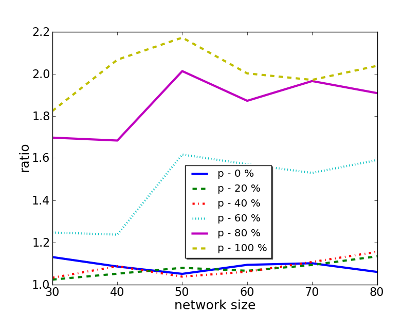
Figure 1: Competitive ratio of Cen as a function of network size and $p$ in a time zone scenario. Results are averaged over 10 runs, we use $\lambda=10$ and collected data over a period of 400 rounds.

The same results for Mix can be seen in Figure 2. Again, larger $p$ yield higher ratios, and generally the performance is worse than the one of Cen.

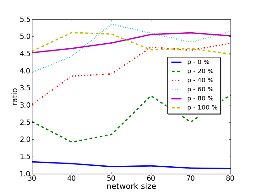
Figure 2: Same experiment as Figure 1 for Mix.

Due to the high time complexity of the optimal offline algorithm, we conducted some experiments with absolute costs only, see Figure 3. Again, the number of requests per round is one fifth of the network size. This reveals an interesting phenomena, namely that in this time zone scenario, Mix becomes better and gets close to the performance of Cen in large networks.

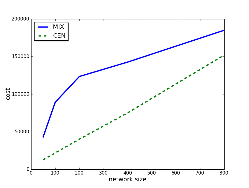
Figure 3: Absolute costs in time zone scenario: $p=40\%$, $\lambda=10$, averaged over 10 runs and studying a runtime of 500 rounds.

Another interesting question regards how the competitive ratio depends on the dynamics, i.e., on $\lambda$. Figure 4 presents our results for Mix and Cen. Although the variance is quite high (this is typical, especially for Mix), we can see a trend that in case of very high dynamics and very low dynamics, the competitive ratio is slightly lower than for $\lambda$ values in-between ($\lambda$ is the mean stay duration). This can be explained by the fact that Opt can optimize relatively more in scenarios where the online migration decisions are not obvious.

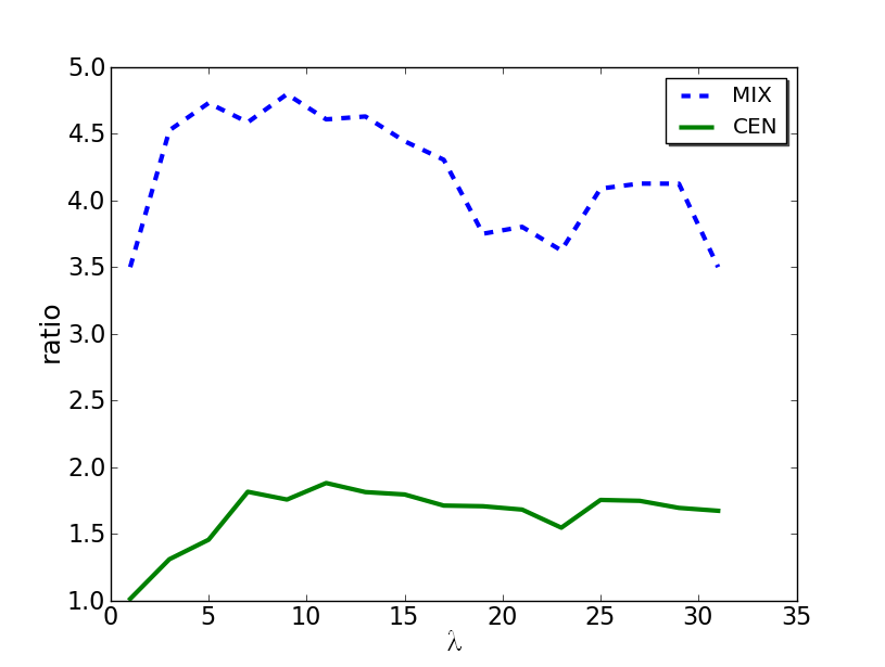
Figure 4: Competitive ratio in time zone scenario (with $p=60\%$) as a function of $\lambda$ and averaged over 10 runs and in a network of 60 nodes. We ran the experiment for 200 rounds.

Generally, in the random graphs of the size used in our experiments, the diameter is relatively low and hence Stat typically has a good performance as well. In the commuter scenario, it is worse than in the time zone scenario. Figure 5 shows that both online algorithms perform very good (and better than in the time-zone scenario).

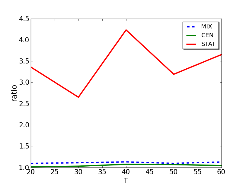
Figure 5: Commuter scenario with $T=3$, server size 30MB $\lambda=10$, runtime 200 rounds and averaged over 20 runs.

One takeaway from our experiments with the different scenarios is that migration is relatively more beneficial in these instances of the commuter scenario compared to the time zone instances studied.

Finally, a note on experiments on Rocketfuel topologies. Also there, the competitive ratios were low. For instance, on the autonomous system AS-7018 of ATT which consists of 115 nodes (see Figure 6), and averaging over 50 runs at a runtime of 100, the optimal offline cost is 477.905648298, Mix has cost of 1179.85 and Cen has cost 825.81, which implies a competitive ratio is around 2.4 and 1.7, respectively. Also Stat performs quite well: without migration the cost lies between Mix and Cen: 1091.51.

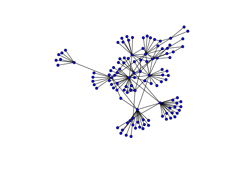
Figure 6: ATT network AS-7018 with 115 nodes.

VI-C Inter Provider Migration

We also conducted some experiments with multiple PIPs. Generally, we used the same random topologies to model a single PIP network, and connected different PIPs in a circular manner using a random connection between adjacent providers.

As in the intra provider scenario, we first report on scalability. Figure 7 plots the competitive ratio as a function of the total number of nodes per provider, given that there are three providers. The ratios are similar to the single PIP case, $\textsc{Mix}_{k}$ is slightly worse than $\textsc{Cen}_{k}$, and constant bandwidth scenarios yield lower ratios.

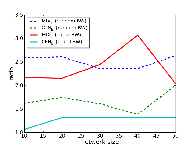
Figure 7: Competitive ratio in time zone scenario (with $p=0\%$) with three providers, server size 30MB, $\lambda=2$ and a runtime of 50 rounds. We average the ratio over five runs.

Figure 8 shows the effect of different correlation ($p$ values) for $\textsc{Cen}_{k}$, and Figure 9 studies the analogous situation for $\textsc{Mix}_{k}$.

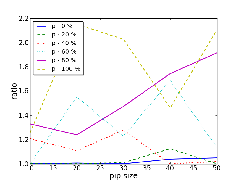
Figure 8: Time zone scenario with three PIPs, $\lambda=5$, runtime 200 rounds: competitive ratio of $\textsc{Cen}_{k}$ as a function of provider size and $p$.

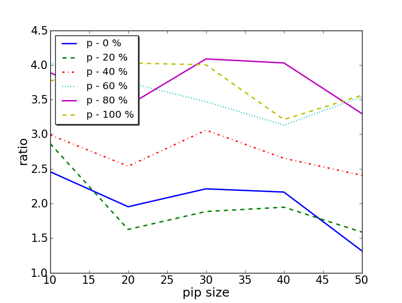
Figure 9: Like Figure 8 but for $\textsc{Mix}_{k}$.

In terms of dynamics, we also have a similar picture as in the single provider case, see Figure 10.

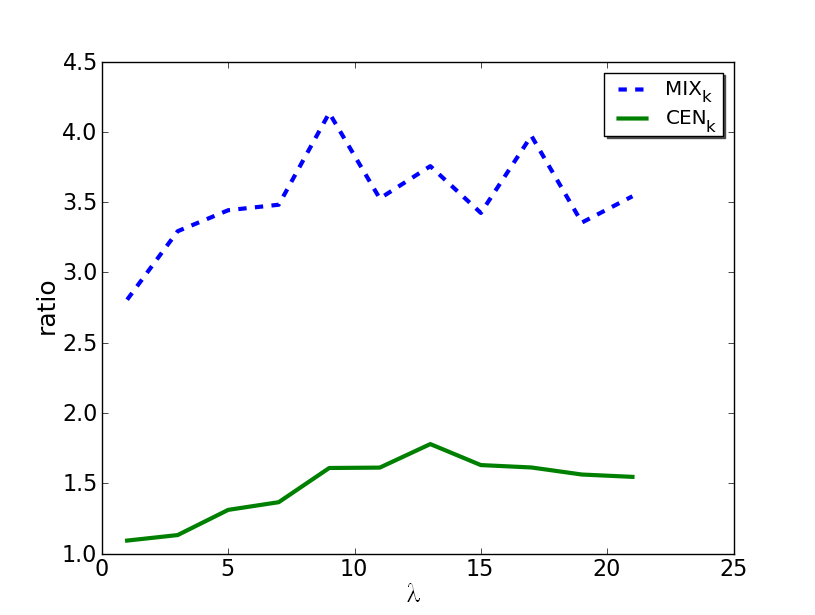
Figure 10: Time zone scenario ($p=60\%$) for three providers with 20 nodes each, runtime 200 and averaged over 10 runs.

It turns out that both $\textsc{Mix}_{k}$ and $\textsc{Cen}_{k}$ are relatively robust to $x=\pi/\beta$, the relative cost of transit compared to migration, although $\textsc{Mix}_{k}$ slightly benefits from lower migration costs, as we would expect (see Figure 11).

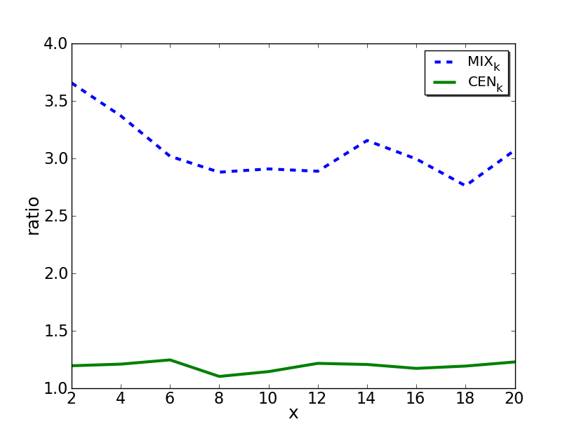
Figure 11: Ratio as a function of $x=\pi/\beta$. Time zone scenario ($p=50\%$) with 3 PIPs, runtime 400, PIP size 20 nodes, $\lambda=5$, averaged over 10 iterations.

Finally, we have studied the competitive ratio as a function of the total number of PIPs. Interestingly, as can be observed in Figure 12, a medium number of providers is slightly worse than scenarios with very few or many providers, but the ratio is pretty robust here as well.

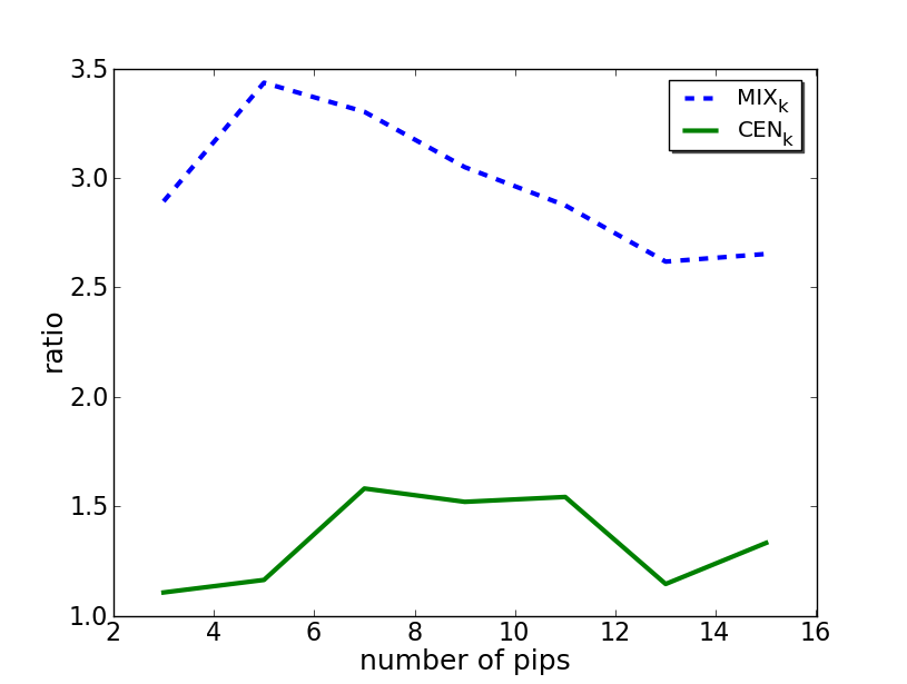
Figure 12: Time zone scenario ($p=50\%$) runtime 400, PIP size 10 nodes, $\lambda=5$, averaged over 10 iterations.

In an experiment with Rocketfuel topologies (network shown in Figure 13), averaging over ten runs, we obtain a total cost of 105.86 for Opt, 356.89 for Mix, and 226.66 for Cen, yielding a competitive ratio of around four for Mix and two for Cen.

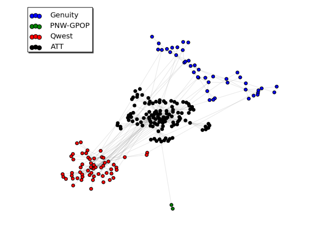
Figure 13: Multi-PIP network with four U.S. providers (217 nodes in total) Genuity (AS-1), PNW-GPOP (AS-101), Qwest (AS-209), and ATT (AS-7018).

VII Conclusion

At the heart of network virtualization lies the ability to react to changing environments in a flexible fashion. In order to optimally exploit the benefits from virtualization, algorithms need to be designed that adapt dynamically to the current demand; this is typically difficult as future demand is hard to predict. We believe that competitive analysis is an important tool to devise and understand such online algorithms.

This paper studied the cost-benefit tradeoff of online migration in a system supported by network virtualization, and compared our system to a setting without migration. We derived the first migration algorithms, both for inter and intra provider scenarios, which are competitive even in the worst-case.

We understand our work as a first step towards a better understanding of competitive virtual service migration, and there are several interesting directions for future research. For instance, we believe that the bounds on the competitive ratio for multiple PIPs are overly pessimistic and can be improved. We also plan to study (simplified versions of) our algorithms in the wild, i.e., in our prototype [31] architecture.

Finally, we emphasize that while our formal considerations may give insights into the benefits of this new technology, e.g., in terms of improved quality of service, whether and how mobile network provider will adapt such an approach also depends on many economic factors that are not taken into account in our model.

References

- [1] D. Arora, A. Feldmann, G. Schaffrath, and S. Schmid. On the benefit of virtualization: Strategies for flexible server allocation. In Proc. USENIX Workshop on Hot Topics in Management of Internet, Cloud, and Enterprise Networks and Services (Hot-ICE), 2011.
- [2] Y. Bartal. Distributed paging. In Dagstul Workshop on On-line Algorithms, pages 97–117, 1996.
- [3] A. Bavier, N. Feamster, M. Huang, L. Peterson, and J. Rexford. In vini veritas: Realistic and controlled network experimentation. In ACM SIGCOMM, 2006.
- [4] S. Bhatia, M. Motiwala, W. Muhlbauer, V. Valancius, A. Bavier, N. Feamster, L. Peterson, and J. Rexford. Hosting virtual networks on commodity hardware. Technical Report GT-CS-07-10, Georgia Tech, 2008.
- [5] M. Bienkowski, A. Feldmann, D. Jurca, W. Kellerer, G. Schaffrath, S. Schmid, and J. Widmer. Competitive analysis for service migration in vnets. In Proc. 2nd ACM SIGCOMM VISA, 2010.
- [6] M. Bienkowski and S. Schmid. Online function tracking with generalized penalties. In Proc. 12th Scandinavian Symposium and Workshops on Algorithm Theory (SWAT), 2010.
- [7] A. Borodin and R. El-Yaniv. Online computation and competitive analysis. Cambridge University Press, 1998.
- [8] A. Borodin, N. Linial, and M. E. Saks. An optimal on-line algorithm for metrical task system. J. ACM, 39(4):745–763, 1992.
- [9] R. Bradford, E. Kotsovinos, A. Feldmann, and H. Schi berg. Live wide-area migration of virtual machines including local persistent state. In Proc. VEE, 2007.
- [10] K. Chowdhury, M. R. Rahman, and R. Boutaba. Virtual network embedding with coordinated node and link mapping. In Proc. INFOCOM, 2009.
- [11] M. Chowdhury, F. Samuel, and R. Boutaba. PolyViNE: Policy-based virtual network embedding across multiple domains. In Proc. 2nd ACM SIGCOMM Workshop on Virtualized Infrastructure Systems and Architecture (VISA), 2010.
- [12] M. K. Chowdhury and R. Boutaba. A survey of network virtualization. Elsevier Computer Networks, 54(5), 2010.
- [13] D. D. Clark, J. Wroclawski, K. R. Sollins, and R. Braden. Tussle in cyberspace: Defining tomorrow’s Internet. In Proc. SIGCOMM, 2002.
- [14] Data from 2008. International Telecommunications Union, 2009.
- [15] G. Even, M. Medina, G. Schaffrath, and S. Schmid. Competitive and deterministic embeddings of virtual networks. In ArXiv Technical Report 1101.5221, 2011.
- [16] J. Fan and M. H. Ammar. Dynamic topology configuration in service overlay networks: A study of reconfiguration policies. In Proc. INFOCOM, 2006.
- [17] D. Fotakis. On the competitive ratio for online facility location. In Proc. 30th International Conference on Automata, Languages and Programming (ICALP), also appeared in Algorithmica 50(1), pp. 1-57, 2008, pages 637–652, 2003.
- [18] C. Guo, G. Lu, H. Wang, S. Yang, C. Kong, P. Sun, W. Wu, and Y. Zhang. Secondnet: A data center network virtualization architecture with bandwidth guarantees. In Proc. ACM CONEXT, 2010.
- [19] F. Hao, T. V. Lakshman, S. Mukherjee, and H. Song. Enhancing dynamic cloud-based services using network virtualization. SIGCOMM Comput. Commun. Rev., 40(1):67–74, 2010.
- [20] U. C. Kozat, Y. Gwon, and R. Jain. An overlay server system (oss) platform for multiplayer online games over mobile networks. In Proc. Global Telecommunications Conference, 2006 (GLOBECOM), 2006.
- [21] N. Laoutaris, G. Smaragdakis, K. Oikonomou, I. Stavrakakis, and A. Bestavros. Distributed placement of service facilities in large-scale networks. In IEEE INFOCOM, 2007.
- [22] J. Lischka and H. Karl. A virtual network mapping algorithm based on subgraph isomorphism detection. In Proc. VISA, pages 81–88, 2009.
- [23] J. Lu and J. Turner. Efficient mapping of virtual networks onto a shared substrate. In Technical Report, WUCSE-2006-35, Washington University, 2006.
- [24] J. R. M. Yu, Y. Yi and M. Chiang. Rethinking virtual network embedding: Substrate support for path splitting and migration. ACM SIGCOMM Computer Communication Review, 38(2):17–29, Apr 2008.
- [25] N. McKeown, T. Anderson, H. Balakrishnan, G. Parulkar, L. Peterson, J. Rexford, S. Shenker, and J. Turner. Openflow: Enabling innovation in campus networks. SIGCOMM Comput. Commun. Rev., 38(2):69–74, 2008.
- [26] B. Monien and H. Sudborough. Embedding one interconnection network in another. In Computational Graph Theory, 1990.
- [27] K.-M. Park and C.-K. Kim. A framework for virtual network embedding in wireless networks. In Proc. 4th International Conference on Future Internet Technologies (CFI), pages 5–7, 2009.
- [28] R. Potter and A. Nakao. Mobitopolo: A portable infrastructure to facilitate flexible deployment and migration of distributed applications with virtual topologies. In Proc. 1st ACM Workshop on Virtualized Infrastructure Systems and Architectures (VISA), pages 19–28, 2009.
- [29] R. Ricci, C. Alfeld, and J. Lepreau. A solver for the network testbed mapping problem. SIGCOMM Comput. Commun. Rev., 33(2):65–81, 2003.
- [30] G. Schaffrath, S. Schmid, and A. Feldmann. Generalized and resource-efficient VNet embeddings with migrations. In ArXiv Technical Report 1012.4066, 2011.
- [31] G. Schaffrath, C. Werle, P. Papadimitriou, A. Feldmann, R. Bless, A. Greenhalgh, A. Wundsam, M. Kind, O. Maennel, and L. Mathy. Network virtualization architecture: Proposal and initial prototype. In Proc. VISA, 2009.
- [32] N. Spring, R. Mahajan, and T. Andersonr. Quantifying the causes of path inflation. In Proc. SIGCOMM, 2003.
- [33] N. Spring, R. Mahajan, D. Wetherall, and T. Anderson. Measuring ISP topologies with rocketfuel. IEEE/ACM Trans. Netw., 12(1):2–16, 2004.
- [34] A. Talukder and R. Yavagal. Mobile Computing: Technology, Applications, and Service Creation. McGraw-Hill, 2006.
- [35] US National Science Foundation. Global environment for network innovations (GENI). http://www.geni.net/, 2006.
- [36] K. Yi and Q. Zhang. Multi-dimensional online tracking. In Proc. of the 19th ACM-SIAM Symp. on Discrete Algorithms (SODA), pages 1098–1107, 2009.
- [37] F. Zaheer, J. Xiao, and R. Boutaba. Multi-provider service negotiation and contracting in network virtualization. In Proc. 12th IEEE/IFIP Network Operations and Management Symposium (NOMS 2010), 2010.
- [38] Y. Zhu and M. H. Ammar. Algorithms for assigning substrate network resources to virtual network components. In Proc. INFOCOM, 2006.