H I CONTENT AND OPTICAL PROPERTIES OF FIELD GALAXIES FROM THE ALFALFA SURVEY. II. MULTIVARIATE ANALYSIS OF A GALAXY SAMPLE IN LOW DENSITY ENVIRONMENTS

Abstract

This is the second paper of two reporting results from a study of the H I content and stellar properties of nearby galaxies detected by the Arecibo Legacy Fast ALFA blind 21-cm line survey and the Sloan Digital Sky Survey in a 2160 square degree region of high galactic latitude sky covered by both surveys, in the general Virgo direction. Here we analyze a complete H I flux-limited subset of 1624 objects with homogeneously measured 21-cm and multi-wavelength optical attributes extracted from the control sample of H I emitters in environments of low local galactic density assembled by Toribio et al. (2010). Strategies of multivariate data analysis are applied to this dataset in order to: i) investigate the correlation structure of the space defined by an extensive set of potentially independent observables describing gas-rich systems; ii) identify the intrinsic parameters that best define their neutral gas content; and iii) explore the scaling relations arising from the joint distributions of the quantities most strongly correlated with the H I mass. The principal component analysis performed over a set of five galaxy properties reveals that they are strongly interrelated, supporting previous claims that nearby H I emitters show a high degree of correlation. The best predictors for the expected value of $M_{\rm{\scriptstyle{H}\,\scriptscriptstyle I}}$ are the diameter of the stellar disk, $D_{25,r}$, followed by the total luminosity (both in the $r$-band), and the maximum rotation speed, while morphological proxies such as color show only a moderately strong correlation with the gaseous content attenuated by observational error. Among the various inferred prescriptions, the simples and most accurate is $\log(M_{\rm{\scriptstyle{H}\,\scriptscriptstyle I}}/M_{\odot})=8.72+1.25\log(D_{25,r}/\mbox{kpc})$. We find a slope of $-8.2\pm 0.5$ for the relation between optical magnitude and log rotation speed, in good agreement with Tully-Fisher studies, as well as a log slope of $1.55\pm 0.06$ for the H I mass-optical galaxy size relation. Given the homogeneity of the measurements and the completeness of our dataset, the latter outcome suggests that the constancy of the average (hybrid) H I surface density advocated by some authors for the spiral population is just a crude approximation.

1 INTRODUCTION

While the literature abounds with attempts of improving our knowledge about the formation and evolution of galaxies from the cross-correlation of the main properties of their baryonic components e.g., Gavazzi, Pierini, & Boselli 1996; Rosenberg, Schneider, & Posson-Brown 2005; Garcia-Appadoo et al. 2009, to name a few representative examples, the possibility of using this sort of relationships to set reference standards for the H I content has received comparatively less attention. Early comparisons of the neutral hydrogen abundance between Virgo cluster and field galaxies put the emphasis on using distance-independent measures, such as the $M_{\rm{\scriptstyle{H}\,\scriptscriptstyle I}}/L$ and $M_{\rm{\scriptstyle{H}\,\scriptscriptstyle I}}/D^{2}$ ratios (e.g., Davies & Lewis, 1973; Chamaraux et al., 1980), $L$ and $D$ being, respectively, the optical luminosity and intrinsic linear diameter at a certain wavelength. Haynes & Giovanelli (1984; hereafter HG84) were the first both to carry out an objective evaluation of the performance of different diagnostic tools for the H I content and to provide a rigorous operational definition of this quantity. With the help of a control sample of 288 galaxies with 21-cm line emission belonging to the Catalogue of Isolated Galaxies (CIG, Karachentseva, 1973), these authors demonstrated that, whatever the Hubble type, the optical linear diameter is the most important diagnostic tool for the H I mass of galaxies. New expressions for the standards of H I content according to HG84’s definition were later derived in an unbiased way by Solanes, Giovanelli, & Haynes (1996) from a larger, integrated H I flux-limited sample of 532 galaxies from the Catalog of Galaxies and Clusters of Galaxies (CGCG, Zwicky et al., 1961-1968) located in the lowest density environments of the Pisces-Perseus supercluster region.

One serious limitation of these studies, carried out in a time when wide-field redshift surveys were still in their infancy, is that they had to deal with heterogeneous datasets of optically selected targets assembled from incomplete catalogs and affected by complex sampling biases that undermined the validity of the results. In this paper and the accompanying one Toribio et al. 2010; hereafter Paper I, we conduct a systematic analysis of the main structural properties of galaxies selected according to their H I-line emission, which in terms of both sampling quality and statistics represents a significant improvement with respect to earlier studies of this kind. Our study grows out from the combination of data from two large surveys that homogeneously map the distribution of extragalactic sources over a significant fraction of the local universe. These are a compilation of all the data from the ongoing Arecibo Legacy Fast ALFA Survey (ALFALFA) blind 21-cm line survey (Giovanelli et al., 2005) gathered so far in the northern Galactic hemisphere, which contains H I measurements distributed in two separate regions of the high Galactic latitude sky that cover a $z$-space volume of about 2160 deg² $\times$ $18,000$ km s^-1, and the Sloan Digital Sky Survey Data Release Seventh (SDSS DR7; Abazajian et al., 2009), which is complemented with additional data from the NYU Value-Added Galaxy Catalog (NYU-VAGC; Blanton et al., 2005).

In Paper I, we deal with the assembly of control samples of ALFALFA galaxies that are expected to show little or no evidence of interaction with their surroundings and, therefore, that are suitable for providing absolute measures of the H I mass. According to the results of this study, the optimal dataset to set up standards for the neutral gas content of galaxies is a sample of 5647 H I emitters found in regions of low local galactic density, as defined by a nearest neighbor approach. A complete 21-cm flux-limited subset of this control sample will be used here (Section 2) with the aim of exploring inter-variable linear correlations and determining the combinations of intrinsic properties that best define the H I mass of gas-rich objects. In the remainder of the present manuscript, we will show first that the galactic stellar size, luminosity, rotation speed, and to a lesser extent the color, are the intrinsic factors most closely related to the H I mass (Section 3), Then, we will apply strategies of non-parametric multivariate data analysis to these variables in order to: determine their correlation structure and the number and orientation of the statistically significant principal components (Section 4.1); establish standards of normalcy for the H I content of galaxies (Section 4.2); and examine the constraints that can be inferred from these relationships on the most firmly established empirical scaling laws for disk galaxies (Section 4.3). Appendix A, briefly discusses two statistical tests implemented in order to assess the completeness limits of the ALFALFA data as a function of integrated H I flux.

The luminosity distances needed to calculate the various distance-dependent structural properties used in this investigation have been inferred within the framework of the standard concordant flat $\Lambda$CDM cosmology with a reduced Hubble constant $h=H_{0}/(100$ km s^-1 Mpc${}^{-1})=0.7$.

2 SAMPLE SELECTION

We use a trimmed version of the Low-Density Environment (LDE) H I galaxy sample assembled in Paper I. The original LDE sample consists of 5647 reliable ALFALFA detections with a signal-to-noise ratio $S/N>4.5$ that have an optical counterpart in the SDSS catalog and that inhabit regions of low local galactic density ($\rho_{6}\leq 0.5\,h^{3}$ galaxies Mpc^-3; see Paper I for details). In order to deal with data of the highest completeness and quality, the present analysis has been restricted, however, to those H I sources designated code 1, i.e., with a $S/N>6.5$, a clean spectral profile, and a good match between the two polarizations independently observed by ALFALFA, for which it can be assumed that the completeness limit is well represented by the detection limit of the survey. Tests of the performance of the signal detection pipeline made by Saintonge (2007) estimate a reliability close $100\%$ for ALFALFA objects above the prescribed $S/N$ threshold and an overall completeness approaching $\sim 90\%$ for those with a narrow observed velocity width ($<150$ km s^-1). In contrast, for the few code 2 sources originally included in the LDE dataset, which have $4<S/N<6.5$, the reliability for detections of narrow signal is reduced to values near $60\%$ and the overall completeness to $\sim 70\%$.

Likewise, we have removed from the parent LDE sample those galaxies located beyond $15,000$ km s^-1, where the ALFALFA survey detection ability drops significantly due to a strong radio frequency interference (RFI) signal from the San Juan airport FAA radar. (We remind the reader that the original LDE dataset is already confined to objects beyond 2000 km s^-1 in order to eliminate the sources with the most uncertain distances and, in particular, a great deal of the kinematic influence of the Virgo cluster.)

The large size of the LDE sample has allowed us to be also demanding when selecting galaxies with favourable inclination angles. Thus, we have taken into account that at low apparent inclinations orientation estimates become more uncertain and are skewed towards larger values by nonaxysimmetric features in the images, ultimately leading to deprojected properties with divergent errors as a face-on orientation is approached, an issue well known in Tully-Fisher studies (e.g. Toribio & Solanes, 2009). Furthermore, the extinction and reddening corrections that must be applied to optical observables are stronger and less reliable for nearly edge-on objects. Accordingly, we have chosen to restrict the present analysis to the 3032 LDE galaxies that, in addition to verifying the above conditions, have also an isophotal $r$-band axial ratio $0.85\geq(b/a)_{r}\geq 0.2$ (equivalent to $30\arcdeg\leq i\leq 80\arcdeg$ for disks of negligible thickness). A detailed analysis of the inclination dependence of the different relationships examined in this work corroborates that all the correlation coefficients vary little within this range of $b/a$. Furthermore, we have attempted to reduce as much as possible the impact of possible outliers on the inferred relationships, which could be significant especially for low H I-mass objects, by excluding galaxies with highly inaccurate SDSS measurements. Although the restrictions on the axial ratio already discard most of the potential optical outliers, an additional $\sim 7$ per cent of the remaining sources were eliminated for this reason.

Last but not least is the fact that ALFALFA is a noise-limited survey, with a sensitivity that depends on the observed source’s H I linewidth, while the correlations that we want to study ideally ought to be inferred from a volume-limited sample. To sidestep the natural bias of blind 21-cm surveys against sources with low fluxes and large velocity widths, we will be dealing with a subset of the LDE sample that includes objects brighter than a stringent integrated H I flux $\geq 1.3$ Jy km s^-1, for which the survey can be considered complete in a statistical sense regardless of line width (see Appendix A). Each galaxy in this restricted dataset will be weighted by the inverse of the maximum effective volume, $V^{\prime}_{\rm max}$, in which it should, on average, have been detected. To calculate the latter, we have taken into account not just the observed integrated flux of the source, its distance, and the adopted sensitivity limit, but also the presence of large-scale structure in the surveyed volume and the loss of signal that result from man-made RFI, which alter locally the survey completeness and therefore the detection probability of the sources. In the remaining of the paper, we will refer to this selection as our H I flux-limited LDE ’high-quality’ galaxy sample (LDE-HQ for short), which totals 1624 gas-rich objects.

3 PARAMETER SELECTION

Central to this work is the search of dependencies between the neutral gas mass content and other intrinsic properties of H I emitters. We have selected the largest possible number of observational parameters that, besides being suitable to characterize gas-rich objects, are inferred from good quality measurements and either publicly available or easy to compute.

3.1 Available Parameters

In our quest for the most relevant galaxian properties that define the H I content, we first review the extensive set of radio and optical parameters that can be inferred from the observables listed by the ALFALFA and SDSS DR7 and NYU-VAGC catalogs, which in some cases provide different estimates of the same attribute (e.g., Petrosian and model magnitudes to measure brightness, isophotal diameter and Petrosian radius to measure the angular size, and so on). After a first screening of all the possible variables available, paying attention to factors such as the relative size of the obsevational errors, as well as the suitability and robustness of the measurements for the kind of galaxies under scrutiny (i.e., blue, late-type, star-forming systems), we select the following properties as the most convenient for our study.

• The two main measures that can be obtained from ALFALFA observations: the 21-cm linewidth of the source at the $50\%$ level of the two peaks, $W_{50}$, and the H I mass, which is estimated from the equation

  $$M_{\rm{\scriptstyle{H}\,\scriptscriptstyle I}}=2.356\times 10^{5}d^{2}F_{\rm{\scriptstyle{H}\,\scriptscriptstyle I}}\;,$$ (1)

  where $F_{\rm{\scriptstyle{H}\,\scriptscriptstyle I}}$ is the 21-cm line flux integral expressed in Jy km s^-1 and $d$ is the cosmological distance to the source in Mpc calculated from the multiattractor flow model of local peculiar velocities developed by Masters (2005). Examination of the variation of H I surface density with axial ratio for ALFALFA galaxies has lead us to neglect the effects of internal H I self-absortion on $F_{\rm{\scriptstyle{H}\,\scriptscriptstyle I}}$. Note that in this paper $W_{50}$ represents the intrinsic width corrected not only for inclination, but also for the effects of redshift broadening and turbulence (see Springob et al., 2005).

  Due to the absence of reliable estimates of the intrinsic axial ratio $q$ of the targets, we choose to use the $r$-band isophotal axial ratio $(b/a)_{r}$ from the SDSS as a proxy for inclination in the calculation of the intrinsic linewidths. The error on inclination corrections arising from taking $q=0$ is in general negligible, except for nearly edge-on objects, which have been removed from our dataset (see Section 2).

• The luminosities (and their corresponding absolute magnitudes) in the five SDSS bands from Petrosian apparent magnitudes. The latter, which are especially suited for bright, extended objects, lead to recover almost all the light from late-type galaxies and around $80\%$ for early types (Blanton et al., 2001). Absolute magnitudes have been corrected to face-on values following Shao et al. (2007). They are not corrected for the seeing effect.

• The 25 mag arcsec^-2 isophotal major-axis diameter, $D_{25}$, in the five SDSS bands, which provide a more continuous measure of the scale of galaxies than the Petrosian radii $R_{50}$ and $R_{90}$. The minimum velocity cutoff of 2000 km s^-1 adopted in Paper I when defining the LDE sample leaves out of the present analysis more than half of the mostly nearby, blue faint objects having unrealistically small isophotal angular radii in the SDSS database.

  Isophotal linear diameters have been corrected for inclination by using transformations of the form

  $$\log D_{25}=\log D_{25}^{\rm{obs}}+\beta\log(b/a)\;,$$ (2)

  where $D_{25}$ and $D_{25}^{\rm{obs}}$ are, respectively, the intrinsic and observed values of this variable in a given band, whereas the coefficient $\beta$ measures the strength of the corresponding attenuation. We note that our corrections are somewhat stronger than those estimated by Maller et al. (2009) from equation 2 for $R_{50}$. For instance, we obtain $\beta_{r}=0.35$ in the $r$-band, while the attenuation for $R_{50,r}$ calculated by the latter authors is 0.20.

• The colors from model magnitudes. Here, we explore the combinations $(u-g)$, $(g-r)$, $(r-i)$, $(i-z)$, $(u-r)$, $(u-i)$, $(u-z)$, $(g-i)$, $(g-z)$, and $(r-z)$.

  The effect of inclination on the colors of our galaxies has been corrected by using the variation of color with axial ratio quoted in Masters et al. (2010). For galaxies with $\log(a/b)<0.7$, we use the straight-line fits listed in their Equation (3), inferred for Galaxy Zoo (GZ) spirals with $R_{90}>10\arcsec$ and a constant extension of these fits for objects with $\log(a/b)>0.7$, as measured in $g$-band. We have not applied the strongest color corrections derived by Masters et al. for systems with smaller apparent sizes, because we have verified that the adopted transformation is enough to make the average intrinsic $(g-r)$ color of ALFALFA sources independent of viewing angle.

• The Sérsic index, $n$, from the NYU-VAGC catalog, which measures the shape of the observed $r$-band luminosity profile of a galaxy fitted using the Sérsic $R^{1/n}$ formula with elliptical isophotes. Available only for galaxies with $r<18$ mag.

• The (inverse) index of light concentration, $C_{59}=R_{50}/R_{90}$, in the five SDSS bands, which ranges from 0 to 1 and is available for the full SDSS DR7 dataset. Not corrected for seeing.

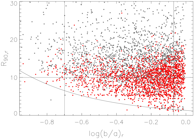
Figure 1: The $r$-band axial ratio versus the radius enclosing 90 per cent of the $r$-band light for galaxies in the ALFALFA LDE sample. Vertical lines correspond to the limits in axial ratio adopted in the definition of the LDE-HQ sample (in red, objects with $F_{\rm{\scriptstyle{H}\,\scriptscriptstyle I}}<1.3$ Jy km s^-1, which we also exclude from the correlation analysis). The horizontal line, plotted at $R_{90,r}=10\arcsec$, marks the limiting radius above which the seeing effects disappear for optical data, while the curved line shows a model in which the minimum possible semiminor axis is $b=1.3\arcsec$, an estimate of the 25th percentile best seeing in the SDSS see Masters et al. 2010.

Along with these variables, we also include the isophotal $(b/a)_{r}$, which given its apparent nature should be uncorrelated with any of the former quantities and can act therefore as a control parameter. The values of this axial ratio quoted in the SDSS are not corrected for seeing, which makes the most inclined galaxies appear rounder than they should be. We note, however, that the possible impact of seeing in our data is likely to be insignificant since its effects are only noticeable for small, highly-inclined galaxies, which are mostly excluded from our sample due the adopted integrated flux cut (the members of the LDE-HQ dataset are regular gas-rich galaxies with $M_{\rm{\scriptstyle{H}\,\scriptscriptstyle I}}\gtrsim 10^{9}\,M_{\odot}$). Besides, blind H I surveys in which the detection probability depends on the observed linewidth like ALFALFA are naturally biased against this kind of targets compare, for instance, the data point densities in our Figure 1 and those in Figure 1 from Masters et al. 2010 derived for GZ spirals.

Note also that in the present analysis, the color, as well as the Sérsic and light concentration indexes, are used as objective proxies of morphology. Attempts to work with ’classical’ indicators of morphological type, such as the continuous de Vaucouleurs numerical code listed in the HyperLeda database, have been thwarted by lack of completeness: about half of the SDSS galaxies do not have information on their Hubble types, while the same is true for $\sim 16\%$ of the ALFALFA sources.

In order to examine the correlation structure, we feed in the logarithms of all these basic variables but $C_{59}$ and $(b/a)_{r}$. In this manner, we should be able to find any scaling law that might exist among them (this is also a must when variables have a lognormal distribution). This means, in particular, that it is not necessary to explicitly include in the analysis interesting composite parameters, such as the stellar mass given by Gavazzi et al. (2008), $\log(M_{\ast}/M_{\odot})=-0.152+0.518\,(g-i)+\log L_{i}$ a similar formula based on the $(g-r)$ color is provided by Bell et al. 2003, that are linear combinations of (the logarithm of) two or more single input variables. This is also the case for the mean surface brightness, isophotal or Petrosian, $\bar{\mu}\,(\equiv M+5\log R)$, which can likewise be expressed as a function of two of the measurements listed above.

3.2 Relevant Parameters

Before we proceed with the present study there is, however, an important consideration that must be taken into account. It has to do with the fact that on a t-test of significance the large size of our sample results in very low critical values for the Pearson’s correlation coefficients, $r_{\rm P}$, i.e., for the elements of the various correlation matrices that are inferred in this section. For instance, $r_{\rm P}^{\rm crit}\sim 0.06$ for a level of significance of 0.01 on a two-tailed test with about 1600 degrees-of-freedom. This implies that variables that ideally should be essentially independent of each other might end up exhibiting a very weak, but nonetheless statistically significant, linear relationship according to this test, even in the presence of attenuation from measurement errors. For this reason, as well as to avoid working with an excessive number of parameters, we have decided to consider that two given properties are truly connected in practice only if they have a Pearson’s $r$ that, aside of being statistically significant, is also minimally strong ($\left|r_{\rm P}\right|>0.3$).

The correlation matrices inferred from different subsets of the attributes selected in Section 3.1 demonstrate that colors and luminosities (absolute magnitudes) are strongly correlated among themselves, as was to be expected. This allows us to discard all but one of the colors and all but one of the luminosities. Among these photometric variables, the ones showing the largest correlation coefficients with the H I mass are the $g$, $r$, and $i$ band luminosities, as well as all the optical colors that can be obtained from combinations of them. Given that the photometric errors in these three bands are rather similar (Strateva et al., 2001), we have taken into account both the dynamic ranges of the different colors and the economy in the number of involved bands to finally select the $r$-band luminosity and the $(g-r)$ color as the most adequate representatives of these two fundamental stellar properties.

The correlation analysis has also evidenced that the available measurements of the isophotal diameter and the Sérsic index in the five SDSS bands are degenerated. As before, the superior quality of the SDSS photometry in the central $g$, $r$, and $i$ bands results in somewhat stronger correlations of these variables with H I mass at such wavelengths. Consistency with the adopted bandpass for measuring the amount of light, has lead us to select $r$-band estimates of $D_{25}$ and $n$ to represent these quantities too.

Overall, we find that the isophotal $r$-band diameter, the $r$-band luminosity, and the $W_{50}$ linewidth are tightly related to the $M_{\rm{\scriptstyle{H}\,\scriptscriptstyle I}}$. A second group of attributes, the $(g-r)$ color and the $r$-band Sérsic index, are moderately aligned with this quantity $\left|r_{\rm P}\right|\sim 0.3$–0.5; see Disney et al. 2008 for a similar conclusion regarding color. While we have decided to retain $(g-r)$ in the set of parameters that may be needed to describe the cold gas content of a galaxy, we have chosen to omit from this list the Sérsic index, as it has a somewhat smaller $\left|r_{\rm P}\right|$ and is available only to galaxies in the NYU-VAGC catalog (i.e., with $r\leq 18$ mag). Finally, the third morphological separator selected, the index of light concentration, shows little or no indication of a major dependence on the H I mass, exhibiting a Pearson’s $r$ of similar strength ($\lesssim 0.2$), for instance, that correlations involving the apparent inclination, so it will also be discarded in the remainder of this study.

4 RELATIONSHIPS AMONG H I AND OPTICAL PROPERTIES

We now complete the characterization of gas-rich galaxies by circumscribing ourselves to the final set of five non-degenerate, intrinsic properties selected in the previous section.

To begin with, we will examine in detail the correlation structure of this multivariate space to both identify its most statistically significant principal components and their degree of alignment with the selected observed parameters. We will then use the correlations among the measured variables to derive formulae for predicting the neutral hydrogen content according to two different approaches. On the one hand, we will seek for the most probable value of $M_{\rm{\scriptstyle{H}\,\scriptscriptstyle I}}$ assuming the other four properties are precisely known. This involves solving a multivariate regression problem in order to obtain equations useful to establish standards of normalcy for the H I content of galaxies —we shall define as ’normal’ the typical values of our LDE-HQ galaxy sample members— from a set of diagnostic parameters easily accessible to observation. On the other hand, we will also determine the best-fitting axes of all the different pairs that can be built from these five basic attributes and the constraints they impose on the scaling laws connecting fundamental properties of galaxies.

4.1 PCA Results

Here we deal with the correlation matrix of the variables $\log(M_{\rm{\scriptstyle{H}\,\scriptscriptstyle I}}\,[M_{\odot}])$, $\log(W_{50}\,[$km s^-1$])$, $\log(D_{25,r}\,[\mbox{kpc}])$, $M_{r}\,[\mbox{mag}]$, and $(g-r)\,[\mbox{mag}]$ in order to perform a principal component analysis (PCA) in this parameter space. Unlike the covariant matrix, the use of the correlation matrix entails the standardization of the original variables putting them on an equal footing: all samples of variables are get to have zero mean and unit standard deviation. This scaling of the measurements avoids the creation of spurious interrelations arising from the preponderance (i.e., larger dynamic range) of certain properties. For the PCA calculations, we employ the IDL procedure pca.pro, implemented following the description by Murtagh & Heck (1987). This algorithm has been modified in order to account for the flux limitation of our sample and the measurement error of the estimates.

As stated in Section 2 (see also Appendix A), the integrated flux cutoff of the LDE-HQ sample has been compensated by weighting each of its member galaxies by the inverse of the maximum volume, $V^{\prime}_{\rm max}$, in which it could have been observed corrected for the systematic effects of large-scale structure and loss of signal due to RFI. This correction is larger for the lowest H I-mass objects since they are only detected at short distance. We have also taken into account that the correlations between variables are weakened in the presence of measurement error. Given two sets of estimates $\hat{X}$ and $\hat{Y}$ with independent measurement errors, the disattenuated correlation between the underlying variables $X$ and $Y$ can be obtained from the formula cf. Spearman 1904

$$r_{\rm P}(X,Y)=\frac{r_{\rm P}(\hat{X},\hat{Y})}{\sqrt{R_{XX}R_{YY}}}\;,$$ (3)

where the reliability coefficients $R_{XX}$ and $R_{YY}$ are defined as one minus the ratio between the variance on the corresponding measurement error and the total observed variance. In practice, this means that variables are standardized using an estimate of their true standard deviation, instead of the observed one. We have followed Fuller & Hidiroglou (1978) see also Bock & Petersen 1975 and extended this correction to the multivariate case by imposing the constraint of producing a valid correlation matrix for our disattenuated variables, i.e., a matrix that is at least positive-semidefinite, after checking that their associated measured error scores are essentially independent.

The results of our PCA analysis are summarized in Tables 1 and 2 in the form of the $1/V^{\prime}_{\rm max}$-weighted correlation matrix, all its eigenvectors and eigenvalues, i.e., the variances of the data in the directions of the principal axes, as well as the rms residuals between the 5-dimensional space (manifold) of the observations and the different $p$-dimensional subspaces ($p=1,...,5$) that best describe them. Table 1, which presents the results for disattenuated correlations, also lists the adopted estimate of the typical measurement error and the square root of the reliability coefficient for the observables. In general, the selected parameters have a near perfect reliability, except the color, for which the attenuation correction is significant.

The correlation matrices indicate the existence of large linear correlations ($|r_{\rm P}|>0.60$) for all pairs of variables except for the H I mass and color, that exhibit correlation coefficients of medium size ($|r_{\rm P}|\sim 0.45$–0.60; note, in contrast, the substantially higher coefficients of the correlations between luminosity and color). Table 1 shows that the five galactic attributes selected are all well correlated with the first principal component. The latter is endowed with direction cosines of nearly equal absolute value ($\approx 1/\sqrt{5}\approx 0.45$) and has an associated eigenvalue $\lambda_{1}$ of $\sim 4.2$, out of a maximum possible of 5.0, implying that about $83\%$ of the total variance in the adopted 5-parameter space can be explained by a single principal axis. The second, and already statistically insignificant, principal component, draws mostly from $M_{\rm{\scriptstyle{H}\,\scriptscriptstyle I}}$, and accounts for an additional $\sim 10\%$ of the global variance, while a linear subspace of three dimensions is enough to explain the practical totality ($\sim 99\%$) of it (these numbers are reduced somewhat when we do not use disattenuated correlation estimates; see Table 2). The principal 4-plane brings the rms residuals down to the level of the adopted observational errors with the exception of $M_{r}$, whose variance cannot be fully accounted for. This might indicate either that there are still hidden parameters controlling the structure of disk galaxies, such as perhaps the mass-normalized star formation rate, which is tightly related to the light concentration index (e.g. Nikolic et al., 2004), or that the observational error adopted for this variable has been too optimistic. Note also that the correlation matrix reveals a very strong negative relationship between the $r$-band magnitude and isophotal diameter, which is responsible for the nearly null variance attached to the last eigenvector.

Our finding that one single principal component —which does not appear to be dominated by any of the five major properties investigated— explains a great deal of the variance of the observed manifold suggests that the structure of regular gaseous galaxies should be determined by very few independent features. This is consistent with the results of earlier PCA-based studies that have attempted to elucidate the degree of organization shown by disk galaxies (e.g. Brosche, 1973; Bujarrabal et al., 1981; Conselice, 2006), as well as in very good agreement with the conclusion that H I galaxies lie essentially on a single fundamental line reached in a recent study by Disney et al. (2008) that, like the present one, combines homogeneous 21-cm data (from the H I Parkes All Sky Survey; HIPASS) with SDSS optical measures.

Regarding the possibility, suggested by these latter authors, that H I-selected galaxies have colors made up of two components, one systematic, correlated with the other variables and the single principal component, and a so-called rogue component, which only alignes with itself and therefore could act as a second significant parameter, we offer a different explanation. Our results —based on a dataset about 8 times larger, though spanning a smaller dynamic range—, show that when the PCA is carried on the attenuated (and $1/V^{\prime}_{\rm max}$-weighted) correlation matrix, we obtain a second principal component, PC2, well aligned with color. Nevertheless, once the measurements are corrected from observational error the color contribution for PC2 significantly weakens and is no longer the dominant one (compare the corresponding eigenvectors in Tables 2 and 1, respectively). This leads us to conclude that the possible statistically significant second degree of freedom found by Disney et al. (2008) is actually an artifact produced by the substantial attenuation exerted by the measurement error of the latter observable on the moderately strong intrinsic H I mass-color correlation (see also Paper I).

4.2 Standards of H I Content

We have just shown that the five observables we are dealing with are actually interconnected. In this situation, any multiple regression model which attempts to describe the H I mass in terms of interrelated predictor variables (multicollinearity) would be associated with an ill-conditioned correlation matrix, i.e., a matrix whose inversion is numerically unstable (if there were one or more exact linear relationships among the variables the matrix would not be invertible). Thus, in the presence of multicollinearity the impact of the individual predictors on the response variable tends to be less precise than if the predictors were uncorrelated with one another. To remedy this problem, we have adopted a two-stage procedure known as Principal Component Regression (PCR; e.g. Cook, 2007) that first carries out a PCA of all the predictor variables, and then uses the resulting principal components —which are independent, and hence associated with a correlation matrix of full rank— together with the dependent variable in an ordinary least squares regression fit. Besides, one can take advantage of the initial PCA transformation to reduce the dimensionality of the data by keeping only those new variables most correlated with the H I mass (e.g. Jolliffe, 1982).

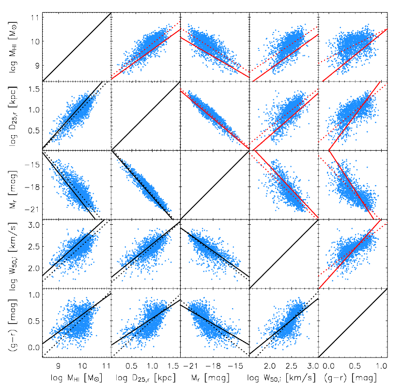
Figure 2: Empirical relations for pairs of properties from LDE-HQ data. $1/V^{\prime}_{\rm max}$-weighted (solid) and unweighted (dotted) direct regression fits to the joint distributions are shown in red color above the diagonal of the plot, whereas orthogonal fits are shown below it. All correlations are corrected for attenuation (Equation 3).

We have applied the above procedure to subspaces of increasing dimension, starting by finding the regression relations between $M_{\rm{\scriptstyle{H}\,\scriptscriptstyle I}}$ and each one of the four remaining properties (see the plots above the diagonal of Figure 2), and then adding input variables progressively to seek for the combinations of regressors that best predict the H I content. This process is stopped when after adding a new predictor variable the rms residual of the multiple regression model increases or does not get reduced in an amount comparable or larger than the typical observational error in $M_{\rm{\scriptstyle{H}\,\scriptscriptstyle I}}$ quoted in Table 1.

In agreement with the results of the previous section, we find that the best predictions for the H I mass are those depending on a single regressor variable. Table 3 lists, ordered according to decreasing accuracy as given by the size of the rms residuals, the central values and associated errors of the coefficients $a_{i}$ of the correlations

$$\log\left(\frac{M_{\rm{\scriptstyle{H}\,\scriptscriptstyle I}}}{M_{\odot}}\right)=a_{0}+a_{1}\;X$$ (4)

for fits with and without $1/V^{\prime}_{\rm max}$-weighting carried on disattenuated data. It can be seen that the most precise predictor of the H I mass is $D_{25,r}$, just the property most strongly correlated with it, followed by $M_{r}$. Among the distance-independent observables, the best predictor of the H I content is the rotational width of the disk, whereas the regression model using the $(g-r)$ color is the least accurate, as expected. Of course, the use of the H I rotation speed to estimate $M_{\rm{\scriptstyle{H}\,\scriptscriptstyle I}}$ only makes sense when the 21-cm line flux integral is not available and this predictor can be replaced by proxies like, for instance, the estimators defined in Catinella et al. (2007) from optical rotation curves.

The uncertainties of the correlation coefficients quoted in Table 3 include two contributions. The first one is the random error, calculated by adding in quadrature the statistical error of the parameter estimates, based on 5000 non-parametric bootstrap trials of the correlations, and the spread due to observational errors, which we have calculated through the creation of 10,000 realizations of the correlations after assigning Gaussian random measurement and distance errors to each galaxy.

The second error term is included to show the impact that voids (and overdensities of comparable size present in the LDE-HQ sample) can have on the inferred relationships by systematically undercounting (overcounting) galaxies in those regions. Remember that we are dealing with galaxies in low-density environments and that the weighting scheme depicted in Appendix A only corrects for the redshift-averaged density of galaxies in the surveyed volume. This systematic error has been evaluated by dividing the sample into 8 equal-area sky regions of $\sim 15\arcdeg$ and calculating the correlations 8 times, leaving out a different section each time. At the median survey redshift of $\sim 8000$ km s^-1, the adopted angular size corresponds to about 30 Mpc, a scale comparable to the typical diameter of voids in the local universe (Hoyle & Vogeley, 2004). The contribution of galaxy under and overdensities to the variance in any correlation coefficient $a_{i}$ is measured through the jackknife error estimator (Lupton, 1993)

$$\sigma^{2}_{a_{i}}=\frac{N-1}{N}\sum_{j=1}^{N}(a_{i,j}-\overline{a_{i}})^{2}\;,$$ (5)

where $N=8$.

Finally, we have also verified that combinations of two distance-dependent input variables, which obey equations of the form

$$\log\left(\frac{M_{\rm{\scriptstyle{H}\,\scriptscriptstyle I}}}{M_{\odot}}\right)=a_{0}+a_{1}\;X_{1}+a_{2}\;X_{2}\;,$$ (6)

do not contribute to reduce the spread that may arise from distance uncertainties. We report in Table 3 the coefficients obtained using the optical size and luminosity as diagnostic variables, which is also the only multilinear regression model with a rms residual as good as that of the best linear model (but at the cost of using two predictors). Looking at the coefficients of this multiple regression for weighted and unweighted data, it is clear that the right-hand side of the equations shows a dependence with distance that neither is null (the ratio $a_{1}/a_{2}\neq-5$), as would be expected if they were defining a surface magnitude, nor does it compensate the $d^{2}$-dependence of the H I mass. As done previously for the single regression models, we account for this breach of distance independence when calculating the random error of the correlation coefficients.

4.3 Planar Correlation Diagrams

In the previous section, we have been interested in obtaining predictions for one integral property, the H I mass, from the observed values of other four ones: size, total magnitude, velocity width, and color. In this section, we turn our attention to the constraints that these intrinsic quantities put on the scaling relations among the fundamental attributes of individual galaxies. This means that we now consider the five compiled variables on an equal footing and focus on the correlations arising from the same PCA technique used in Section 4.1 applied to pairs of them. The involved quantities are therefore treated symmetrically, thus minimizing the inconsistencies that may arise from the possible ’non-commutativity’ of the inferred relationships. The coefficients of the $1/V^{\prime}_{\rm max}$-weighted and unweighted orthogonal fits of the form $Y=a_{0}+a_{1}\;X$ between all 10 possible pairs of galaxy properties are presented in Table 4 for disattenuated data. (For this exercise, the quoted uncertainties depict only the random error estimates calculated as in Section 4.2.) The scatter plots and their best linear fits can be visualized in the boxes below the diagonal in Figure 2.

The study of the scalings of the most basic properties of galaxies is central for constraining theories of their formation and evolution. It has generated an abundant literature, whose detailed revision far exceeds the scope of the present work. Instead, we have decided to focus on the comparison between the values for the mean slopes of the strongest correlations we predict, which are those in the $L(M)RV$ subspace of luminosity (mass), size, and rotation speed, and those reported in other studies that also combine H I and optical observations HG84; Salpeter & Hoffman 1996, or that specifically study the scalings among the above fundamental properties in late-type objects (Courteau et al., 2007). When comparing results allowance should be made not just for differences in sample size, but also for other factors such as the waveband of the optical observations, the specific observables chosen to estimate the above attributes, their dynamic ranges, or the fitting method employed. Another complication that distorts the comparison among the different outcomes is the incompleteness of the datasets that, with the exception of ours, are all affected by intractable selection biases.

With all these caveats in mind, the agreement between the central values of the slopes (rounded to the two most significant digits) reported by the different studies listed above (see Table 5) can be classified as generally satisfactory. The largest discrepancies correspond to the correlation involving the luminosity versus the rotation speed, i.e., the Tully-Fisher (TF) relation, reflecting the fact that it is always problematic to accurately find the slope of this empirical law due to the low dynamic range in $\log V$. The mean values of the log slope $\gamma$ listed in Table 5 range from $\sim 2.6$ $-6.5$ in magnitude units; HG84 to $\sim 3.4$ (Courteau et al., 2007) and $\sim 3.7$ (Salpeter & Hoffman, 1996) (the first and the last ones being measured at blue wavelengths and the Courteau et al.’s for the $I$-band). From our weighted data, we get a slope of $3.3\pm 0.2$ (random error) or, equivalently, $-8.2\pm 0.5$ mag, which roughly falls in the middle of this range and is fully consistent with estimates reported in TF-specific literature for bright spirals in the blue/near-IR band (e.g. Willick et al., 1997; Giovanelli et al., 1997; Courteau, 1997; Masters et al., 2006).

Among all the results obtained, the most striking is perhaps the relationship between the H I mass and the characteristic size of the stellar distribution of gaseous galaxies, represented here by the isophotal diameter in the $r$-band, $D_{25,r}$. Our finding that it has a central slope $\alpha=1.55\pm 0.06$ does not support the idea that all H I-rich galaxies have roughly the same global H I column density, as recently advocated by Garcia-Appadoo et al. (2009, see also references therein) from a sample of HIPASS galaxies and implied by correlations such as the one found by Salpeter & Hoffman (1996), listed in Table 5, from optical size measurements in the $B$-band. (Implicit in this conclusion is the assumption that H I and stellar disk sizes are roughly proportional as shown by Broeils & Rhee (1997).) We remind the reader once again that none of these previous studies based their conclusions on correlation analyses performed on complete multivariate datasets, as we have done here. In particular, we suspect that the use of samples largely dominated by late-type spirals, which are more prone to exhibit a nearly constant mean H I surface density, may contribute to exacerbate the tendency to find such an aesthetically appealing result see also Solanes et al. 1996. In this regard, we wish to emphasize that the claimed constancy of the mean H I column density by Garcia-Appadoo et al. (2009), who deal with a sample that, morphologically speaking, is representative of the entire population of H I emitters, emanates from a (unweighted) H I mass-$R_{50,g}$ correlation with an actual central slope of $\sim 1.7$, in pretty good agreement with our outcome.

5 SUMMARY AND CONCLUDING REMARKS

We have sought for correlations among a large set of extensive 21-cm and optical homogeneous measures available for the 1624 members of a complete, H I flux-limited sample of non-clustered, gas-rich galaxies, not influenced by their environment. Our main aim has been identifying the combinations of intrinsic variables directly arising from observable quantities that make up the best diagnostic tools for the H I content. The sources used for this research have been selected from the Low Density Environment H I galaxy sample of the ALFALFA blind H I survey defined in Paper I. The size of this primary database has been reduced to include only high-quality ALFALFA detections with a $S/N>6.5$ found up to $15,000$ km s^-1 and with moderate inclinations $0.85\geq b/a\geq 0.2$ ($30\arcdeg\leq i\leq 80\arcdeg$ for $q=0$). Furthermore, we have selected only those H I emitters with an integrated flux $\geq 1.3$ Jy km s^-1 from which the sensitivity of the survey becomes essentially independent of profile width.

The examination of the correlation structure of these data, conveniently weighted to compensate for the flux limitation, as well as for the systematic effects of large-scale structure and loss of signal due to man-made RFI in the surveyed volume, has produced the following interesting results.

• In (bright) gas-rich galaxies the isophotal $r$-band linear diameter, total $r$-band luminosity, $W_{50}$ linewidth, and $(g-r)$ color are the galaxian properties most tightly correlated with the total H I mass. The principal component analysis of the manifold defined by these variables has revealed relationships with large correlation coefficients that are suggestive of a high degree of organization in the LDE-HQ sample. This is consistent with the idea that H I emitters behave essentially as a one-parameter family. As previously noted by Disney et al. (2008) see also van den Bergh 2008 and references therein, the observed structural simplicity of disk galaxies is difficult to reconcile with the prevailing theory of hierarchical galaxy formation, which holds that the physical properties of these objects are determined by the interplay of several potentially independent factors, such as mass, spin and (the chaotic at high redshift) merger history of galactic halos.

• In accordance with the output of the PCA, we have found that the best predictions for the most probable value of $M_{\rm{\scriptstyle{H}\,\scriptscriptstyle I}}$, assuming that the regressor variables are precisely known, are those depending on a single parameter. Our fits carried on $1/V^{\prime}_{\rm max}$-weighted and disattenuated data show that the most accurate predictor for the H I mass of a galaxy is its optical diameter, through the equation

  $$\log\left(\frac{M_{\rm{\scriptstyle{H}\,\scriptscriptstyle I}}}{M_{\odot}}\right)=8.72\pm 0.06\pm 0.06+1.25\pm 0.06\pm 0.07\log\left(\frac{D_{25,r}}{\mbox{kpc}}\right)\;,$$ (7)

  where the first error term is statistical and the second the systematic uncertainty arising from the large scale structure present in the surveyed volume. In Table 3, we provide alternative prescriptions to calculate $M_{\rm{\scriptstyle{H}\,\scriptscriptstyle I}}$ from $M_{r}$, $W_{50}$, and $(g-r)$, as well as from a combination of $D_{25,r}$ and $M_{r}$. The fact that the models based on the crude morphological indicator $(g-r)$ yield rms residuals comparable to the global standard deviation associated with $M_{\rm{\scriptstyle{H}\,\scriptscriptstyle I}}$ hints that the morphology of H I emitters plays a secondary role in determining their neutral gas content, as already inferred by HG84 and Solanes et al. (1996).

• From the joint distributions of the quantities most strongly correlated with the H I mass, we derive the mean relationships

  $$M_{\rm{\scriptstyle{H}\,\scriptscriptstyle I}}\propto R^{1.6}\mbox{,\ }M_{\rm{\scriptstyle{H}\,\scriptscriptstyle I}}\propto L^{0.60}\mbox{,\ }L\propto V^{3.3}\mbox{,\ }R\propto L^{0.40}\mbox{,\ }R\propto V^{1.3}\;,$$ (8)

  where $L$ represents the total $r$-band luminosity of the (old) stellar disk of a galaxy, and $R$ and $V$ its size and rotation speed, respectively. Among the scaling relations that involve H I measurements, the most interesting ones are the well-known $LV$ or TF relation and the ratio between the total neutral gas mass and optical radius. For the former, it is noteworthy that we find a central slope fully consistent with the typical values reported in TF studies at optical/near-IR wavelengths from data that have not been specifically selected for this task. On the other hand, the slope inferred for the second scaling implies that the hybrid surface density of neutral hydrogen ($\propto M_{\rm{\scriptstyle{H}\,\scriptscriptstyle I}}/R^{2}$) is not constant, but moderately decreasing with galaxy size. Claims in favor of the near universality of the global H I surface density for the entire spiral population rely on incomplete datasets biased towards galaxies of the latest Hubble subtypes (mostly Sc and Irr), for which the constancy of this intensive property is a relatively acceptable approximation.

To date, most multidimensional statistical studies focusing on the interrelations among the main properties of galaxies have had to contend with largely incomplete, heterogeneous samples of modest size and affected by important selection artifacts. It is therefore evident that disregarding any of these factors when they are in fact present may result in inconsistent estimation. In this respect, efforts like the present one based on the cross-correlation of large datasets assembled from objective, wide-area surveys with controlled sampling biases should mark the way forward.

Appendix A ASSESSING THE INTEGRATED H I FLUX COMPLETENESS OF THE ALFALFA DATA

Although the ALFALFA catalog and its LDE subset are noise-limited datasets, it is possible to define an integrated flux limit, $F_{\rm{\scriptstyle{H}\,\scriptscriptstyle I,lim}}$, above which the confirmed H I sources are not subject on average to the same bias against broad linewidths.

With this aim, we have used the adaptation of the Rauzy (2001) completeness test to a H I-selected galaxy sample by Zwaan et al. (2004), which we briefly recap here. Rauzy’s method, which is not affected by the presence of clustering or by subsampling in redshift bins, relies on the calculation for each galaxy $i$ of the quantity

$$\hat{\zeta}_{i}=\frac{r_{i}}{n_{i}+1}\;,$$ (A1)

which provides an unbiased estimate of the random variable $\zeta_{i}$ that compares the amount of galaxies with more and less neutral hydrogen than every galaxy in the sample under the assumption that the shape of the H I mass function is universal (i.e., invariant in time and position). In equation A1, $r_{i}$ is the number of galaxies with $M_{\rm{\scriptstyle{H}\,\scriptscriptstyle I}}\geq M_{\rm{\scriptstyle{H}\,\scriptscriptstyle I},i}$ and $Z\leq Z_{i}$, $n_{i}$ is the number of galaxies for which $M_{\rm{\scriptstyle{H}\,\scriptscriptstyle I}}\geq M_{\rm{\scriptstyle{H}\,\scriptscriptstyle I},lim}(Z_{i})$ and $Z\leq Z_{i}$, while $Z\equiv\log F_{\rm{\scriptstyle{H}\,\scriptscriptstyle I}}-\log M_{\rm{\scriptstyle{H}\,\scriptscriptstyle I}}$ is a distance measure, and $M_{\rm{\scriptstyle{H}\,\scriptscriptstyle I},lim}(Z_{i})$ is the limiting H I mass at the distance corresponding to $Z_{i}$.

Taking into account that $\zeta_{i}$ is uniformly distributed between 0 and 1 with expectation and variance $E_{i}=1/2$ and $V_{i}=(n_{i}-1)/[12(n_{i}+1)]$, respectively, the principle of the test is to evaluate the variation with decreasing $F_{\rm{\scriptstyle{H}\,\scriptscriptstyle I,lim}}$ of the statistic

$$T_{\rm C}=\frac{\sum_{i=1}^{N_{\rm gal}}(\hat{\zeta}_{i}-1/2)}{\left(\sum_{i=1}^{N_{\rm gal}}V_{i}\right)^{1/2}}\;,$$ (A2)

which follows a Gaussian distribution of zero mean and unit variance under the null hypothesis, H0, that the sample is complete up to a given integrated flux and drops systematically to values below zero when H0 is not fulfilled. The completeness limit can be therefore set by imposing that $T_{\rm C}$ exceeds a given negative value, being $T_{\rm C}<-2$ and $T_{\rm C}<-3$, which correspond to a 97.7 and 99.4 confidence levels of rejection of H0, respectively, the standard decision rules.

Figure 3 shows the results obtained when the test is applied to subsamples of both the ALFALFA data without any density restriction (top panel) and the LDE dataset (bottom panel) truncated to decreasing values of $F_{\rm{\scriptstyle{H}\,\scriptscriptstyle I,lim}}$. Note that for both datasets we are considering only code 1 sources within the bandpass limits 2000 and 15,000 km s^-1 (see Section 2), a subsampling in redshift that should not affect the outcome. It is clear from this figure that if we choose a $-3\sigma$ criterion to reject the completeness hypothesis, which corresponds to the level from which the $T_{\rm C}$ statistic initiates a systematic, sharp decline, the completeness limit of the two samples can be safely set at $1.3$ Jy km s^-1.

A more direct, but less accurate, method to infer whether a survey is complete or not to a given flux limit is to compute the average $V/V_{\rm max}$ of the data, which should be equal to $1/2$ provided that the effective search volume of each galaxy, or equivalently, its detection probability, is accurately established. The $\langle V/V_{\rm max}\rangle$ test presupposes that the galaxies are on average homogeneously distributed and is therefore sensitive to selection and large-scale structure effects. Therefore, the correct application of this second technique to the above H I datasets requires that in the calculation of the individual search volumes we account for the true density of targets as a function of redshift, as well as for the artificial annular underdensities that arise from man-made radio-frequency interferences.

Accordingly, we have modified $V$ and $V_{\rm max}$ in order to include weighting by the average density interior to the corresponding radial distances normalized to the average density within the surveyed volume. The weights have been calculated from a volume-limited subsample of the spectroscopic SDSS DR7 dataset, which is complete to a Petrosian $r$-band magnitude of 17.77, selected to include only galaxies obeying Maller et al. (2009)’s disk criterion, which is very effective identifying objects structurally similar to H I emitters (see Paper I). In addition, we have corrected for RFI by using the same average relative weight as a function of observed heliocentric velocity depicted in Figure 6 by Martin et al. (2010).

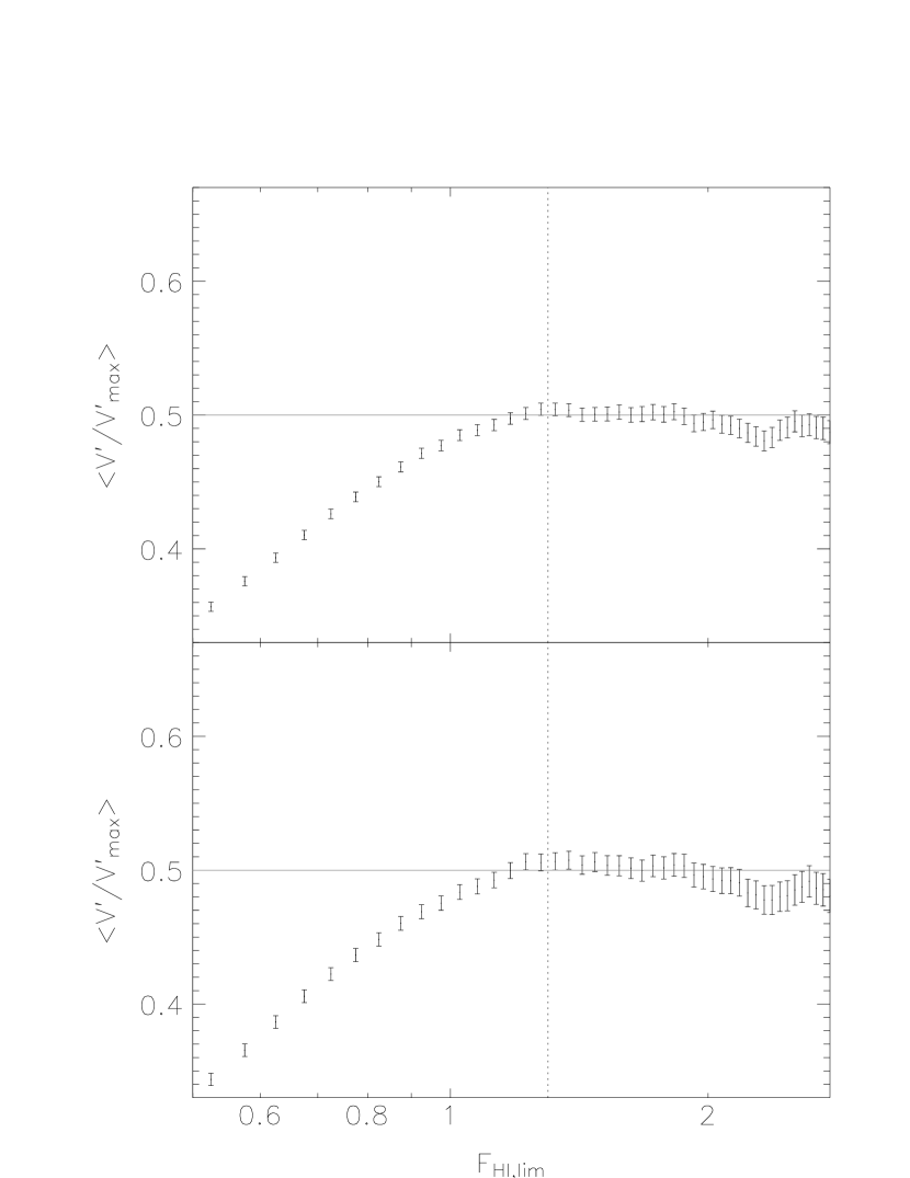
Figure 4: Same as in Figure 3, but for the $\langle V^{\prime}/V^{\prime}_{\rm max}\rangle$ completeness test.

In Figure 4, we depict the expectation value and dispersion of the average ratio of weighted volumes, $\langle V^{\prime}/V^{\prime}_{\rm max}\rangle$, as a function of the integrated H I flux. As we have done previously for Rauzy’s test, we show results for the ALFALFA data (top panel) and its LDE subset (bottom panel; in this case, the radial run of the density weighting is estimated using Maller et al.’s disks in low density environments). Galaxies not belonging to the redshift range 2000–$15,000$ km s^-1 or classified as code 2 detections have been discarded. In very good agreement with the $T_{\rm C}$ method, we find that above $F_{\rm{\scriptstyle{H}\,\scriptscriptstyle I,lim}}\approx 1.3$ Jy km s^-1 the values of this statistic remain, for the two datasets, practically constant around 0.50. Note that the observed rough invariance of $\langle V^{\prime}/V^{\prime}_{\rm max}\rangle$ above this integrated-flux limit supports the assertion that the two samples are statistically complete, while the fact that the observed value of the statistic is so close to its expectation indicates that the effects of large-scale structure and RFI have been correctly averaged out with the adopted weighting strategy and, therefore, that we are dealing with homogeneous datasets.

Table 1: Principal Component Analysis of H I and Optical Properties for Weighted Data and Disattenuated Correlations

	$\log M_{\rm{\scriptstyle{H}\,\scriptscriptstyle I}}$	$\log W_{50}$	$\log D_{25,r}$	$M_{r}$	$(g-r)$	$C_{59,r}$	$(b/a)_{r}$
$\log M_{\rm{\scriptstyle{H}\,\scriptscriptstyle I}}$	1.00	0.65	0.80	$-$0.74	0.58	$-$0.18	0.11
$\log W_{50}$		1.00	0.71	$-$0.76	0.88	$-$0.22	0.08
$\log D_{25,r}$			1.00	$-$0.96	0.85	$-$0.09	0.02
$M_{r}$				1.00	$-$0.87	0.25	$-$0.00
$(g-r)$					1.00	$-$0.19	0.20
$C_{59,r}$						1.00	0.10
$(b/a)_{r}$							1.00
Mean ($N_{\rm gal}=1624$)	8.82	2.22	0.42	$-$17.43	0.33	0.44	0.50
Standard dev.	0.36	0.18	0.23	1.48	0.12	0.05	0.16
Observational error	0.02	0.03	0.05	0.10	0.10	0.01	0.07
$\sqrt{R_{XX}}$	1.00	0.99	0.98	1.00	0.79	0.98	0.92
Eigenvectors						Eigenvalues (%)
$\hat{\mbox{\boldmath$e$}}_{1}$	0.40	0.43	0.47	$-$0.47	0.46	$\lambda_{1}=$ 4.17	(83.31)
$\hat{\mbox{\boldmath$e$}}_{2}$	0.73	$-$0.45	0.21	$-$0.03	$-$0.46	$\lambda_{2}=$ 0.49	(93.02)
$\hat{\mbox{\boldmath$e$}}_{3}$	0.46	0.63	$-$0.43	0.43	$-$0.12	$\lambda_{3}=$ 0.30	(99.07)
$\hat{\mbox{\boldmath$e$}}_{4}$	$-$0.08	0.21	$-$0.41	$-$0.75	$-$0.47	$\lambda_{4}=$ 0.05	(100)
$\hat{\mbox{\boldmath$e$}}_{5}$	$-$0.29	0.40	0.62	0.17	$-$0.58	$\lambda_{5}=$ 0.00	(100)
rms residuals:
Principal Axis	0.22	0.09	0.09	0.51	0.09
Principal Plane	0.11	0.09	0.07	0.50	0.06
Princ. 3-Plane	0.06	0.05	0.05	0.42	0.06
Princ. 4-Plane	0.05	0.04	0.07	0.12	0.04
Princ. 5-Plane	0.00	0.00	0.00	0.00	0.00

Note. — PCA is carried on the first 5 properties only: $\log(M_{\rm{\scriptstyle{H}\,\scriptscriptstyle I}}\,[M_{\odot}])$, $\log(W_{50}\,[\mbox{\mbox{km\ s}${}^{-1}$}])$, $\log(D_{25,r}\,[\mbox{kpc}])$, $M_{r}\,[\mbox{mag}]$, and $(g-r)\,[\mbox{mag}]$.

Table 2: Principal Component Analysis of H I and Optical Properties for Weighted Data

	$\log M_{\rm{\scriptstyle{H}\,\scriptscriptstyle I}}$	$\log W_{50}$	$\log D_{25,r}$	$M_{r}$	$(g-r)$	$C_{59,r}$	$(b/a)_{r}$
$\log M_{\rm{\scriptstyle{H}\,\scriptscriptstyle I}}$	1.00	0.64	0.78	$-$0.73	0.46	$-$0.17	0.10
$\log W_{50}$		1.00	0.69	$-$0.75	0.69	$-$0.21	0.07
$\log D_{25,r}$			1.00	$-$0.94	0.66	$-$0.09	0.02
$M_{r}$				1.00	$-$0.69	0.24	$-$0.00
$(g-r)$					1.00	$-$0.15	0.14
$C_{59,r}$						1.00	0.09
$(b/a)_{r}$							1.00
Mean ($N_{\rm gal}=1624$)	8.82	2.22	0.42	$-$17.43	0.33	0.44	0.50
Standard dev.	0.36	0.18	0.23	1.48	0.12	0.05	0.16
Eigenvectors						Eigenvalues (%)
$\hat{\mbox{\boldmath$e$}}_{1}$	0.42	0.44	0.48	$-$0.48	0.41	$\lambda_{1}=$ 3.83	(76.57)
$\hat{\mbox{\boldmath$e$}}_{2}$	0.61	$-$0.25	0.21	$-$0.09	$-$0.72	$\lambda_{2}=$ 0.57	(88.06)
$\hat{\mbox{\boldmath$e$}}_{3}$	$-$0.25	$-$0.78	0.43	$-$0.31	0.23	$\lambda_{3}=$ 0.33	(94.60)
$\hat{\mbox{\boldmath$e$}}_{4}$	$-$0.61	0.34	0.20	$-$0.45	$-$0.52	$\lambda_{4}=$ 0.22	(98.98)
$\hat{\mbox{\boldmath$e$}}_{5}$	$-$0.14	0.15	0.71	0.67	$-$0.05	$\lambda_{5}=$ 0.05	(100)
rms residuals:
Principal Axis	0.20	0.09	0.08	0.48	0.10
Principal Plane	0.12	0.09	0.07	0.47	0.04
Princ. 3-Plane	0.10	0.03	0.04	0.39	0.04
Princ. 4-Plane	0.01	0.01	0.04	0.23	0.00
Princ. 5-Plane	0.00	0.00	0.00	0.00	0.00

Note. — PCA is carried on the first 5 properties only: $\log(M_{\rm{\scriptstyle{H}\,\scriptscriptstyle I}}\,[M_{\odot}])$, $\log(W_{50}\,[\mbox{\mbox{km\ s}${}^{-1}$}])$, $\log(D_{25,r}\,[\mbox{kpc}])$, $M_{r}\,[\mbox{mag}]$, and $(g-r)\,[\mbox{mag}]$.

Table 3: Coefficients of $M_{\rm{\scriptstyle{H}\,\scriptscriptstyle I}}$ Predictions from Single and Multiple Linear Regression Models

Weighting	$X_{1}$	$X_{2}$	$a_{0}$			$a_{1}$			$a_{2}$			Residual
$1/V^{\prime}_{\rm max}$	$\log D_{25,r}$		8.72	$\pm 0.06$	$\pm 0.06$	1.25	$\pm 0.06$	$\pm 0.07$				0.23
	$M_{r}$		6.44	$\pm 0.20$	$\pm 0.21$	$-$0.18	$\pm 0.01$	$\pm 0.01$				0.25
	$\log W_{50}$		6.54	$\pm 0.27$	$\pm 0.20$	1.30	$\pm 0.11$	$\pm 0.09$				0.28
	$(g-r)$		8.84	$\pm 0.11$	$\pm 0.12$	1.81	$\pm 0.29$	$\pm 0.40$				0.33
	$\log D_{25,r}$	$M_{r}$	7.26	$\pm 0.12$	$\pm 0.04$	0.66	$\pm 0.03$	$\pm 0.01$	$-$0.10	$\pm 0.006$	$\pm 0.002$	0.22
None	$\log D_{25,r}$		8.85	$\pm 0.04$	$\pm 0.03$	1.37	$\pm 0.04$	$\pm 0.03$				0.21
	$M_{r}$		6.44	$\pm 0.09$	$\pm 0.08$	$-$0.20	$\pm 0.004$	$\pm 0.002$				0.23
	$\log W_{50}$		7.17	$\pm 0.14$	$\pm 0.16$	1.21	$\pm 0.05$	$\pm 0.06$				0.28
	$(g-r)$		9.61	$\pm 0.04$	$\pm 0.04$	1.10	$\pm 0.08$	$\pm 0.07$				0.32
	$\log D_{25,r}$	$M_{r}$	6.89	$\pm 0.05$	$\pm 0.02$	0.61	$\pm 0.01$	$\pm 0.005$	$-$0.10	$\pm 0.002$	$\pm 0.001$	0.23

Table 4: Coefficients of Orthogonal Fits between Pairs of Variables

		$X$
Weighting	$Y$	$\log D_{25,r}$		$M_{r}$		$\log W_{50}$		$(g-r)$
		$a_{0}$	$a_{1}$	$a_{0}$	$a_{1}$	$a_{0}$	$a_{1}$	$a_{0}$	$a_{1}$
$1/V^{\prime}_{\rm max}$	$\log M_{\rm{\scriptstyle{H}\,\scriptscriptstyle I}}$	8.55$\pm 0.05$	1.55$\pm 0.06$	5.36$\pm 0.19$	$-$0.24$\pm 0.010$	5.01$\pm 0.30$	1.99$\pm 0.13$	8.45$\pm 0.12$	2.99$\pm 0.29$
	$\log D_{25,r}$			$-$2.05$\pm 0.09$	$-$0.16$\pm 0.004$	$-$2.28$\pm 0.21$	1.29$\pm 0.14$	$-$0.06$\pm 0.06$	1.93$\pm 0.15$
	$M_{r}$					1.46$\pm 1.14$	$-$8.15$\pm 0.48$	$-$12.8$\pm 0.40$	$-$12.2$\pm 0.98$
	$\log W_{50}$							1.73$\pm 0.06$	1.50$\pm 0.13$
None	$\log M_{\rm{\scriptstyle{H}\,\scriptscriptstyle I}}$	8.58$\pm 0.03$	1.66$\pm 0.03$	5.24$\pm 0.08$	$-$0.26$\pm 0.004$	5.30$\pm 0.11$	1.98$\pm 0.04$	9.06$\pm 0.04$	2.28$\pm 0.07$
	$\log D_{25,r}$			$-$2.02$\pm 0.03$	$-$0.16$\pm 0.002$	$-$1.98$\pm 0.08$	1.19$\pm 0.03$	0.29$\pm 0.02$	1.38$\pm 0.03$
	$M_{r}$					$-$0.24$\pm 0.42$	$-$7.57$\pm 0.16$	$-$14.6$\pm 0.13$	$-$8.74$\pm 0.26$
	$\log W_{50}$							1.90$\pm 0.01$	1.15$\pm 0.04$

Table 5: Central Slopes of Scaling Laws between Fundamental Galaxian Properties Reported by Different Authors

Reference	Scaling law
	$M_{\rm{\scriptstyle{H}\,\scriptscriptstyle I}}\sim R^{\alpha}$	$M_{\rm{\scriptstyle{H}\,\scriptscriptstyle I}}\sim L^{\beta}$	$L\sim V^{\gamma}$	$R\sim L^{\delta}$	$R\sim V^{\epsilon}$
HG84 (1984)	1.8	0.66	2.6	$\cdots$	$\cdots$
Salpeter & Hoffman (1996)	2.0	0.74	3.7	0.37	1.4
Courteau et al. (2007)	$\cdots$	$\cdots$	3.4	0.32	1.1
This work	1.6	0.60	3.3	0.40	1.3

Figure 3: Rauzy’s test for completeness applied to data from the ALFALFA survey (top) and from its LDE subset (bottom). We only consider code 1 sources with redshifts between 2000 and 15,000 km s^-1. In both cases, the H I flux completeness limit, $F_{\rm{\scriptstyle{H}\,\scriptscriptstyle I,lim}}$, (determined by $T_{\rm C}=-3$) falls somewhat below $1.3$ Jy km s^-1 (vertical dotted line).

References

- Abazajian et al. (2009) Abazajian, K. N., et al. 2009, ApJS, 182, 543
- Allam et al. (2005) Allam, S. S., Tucker, D. L., Lee, B. C., & Smith, J. A. 2005, AJ, 129, 2062
- Baldry et al. (2004) Baldry, I. K., Glazebrook, K., Brinkmann, J., Ivezić, Ž., Lupton, R. H., Nichol, R. C., & Szalay, A. S. 2004, ApJ, 600, 681
- Ball et al. (2008) Ball, N. M., Loveday, J., & Brunner, R. J. 2008, MNRAS, 383, 907
- Balogh et al. (1998) Balogh, M. L., Schade, D., Morris, S. L., Yee, H. K. C., Carlberg, R. G., & Ellingson, E. 1998, ApJ, 504, L75
- Bamford et al. (2009) Bamford, S. P., et al. 2009, MNRAS, 393, 1324
- Bell et al. (2003) Bell, E. F., McIntosh, D. H, Katz, N., & Weinberg, M. D. 2003, ApJS, 149, 289
- Blanton et al. (2001) Blanton, M. R., et al. 2001, AJ, 121, 2358
- Blanton et al. (2003) Blanton, M. R., et al. 2003, ApJ, 594, 186
- Blanton et al. (2005) Blanton, M. R., et al. 2005, AJ, 129, 2562
- Bock & Petersen (1975) Bock, R. D., & Petersen, A. C. 1975, Biometrika, 62, 673
- Broeils & Rhee (1997) Broeils, A. H., & Rhee, M.-H. 1997, A&A, 324, 877
- Brosche (1973) Brosche, P. 1973, A&A, 23, 259
- Bujarrabal et al. (1981) Bujarrabal, V., Guibert, J., & Balkowski, C. 1981, A&A, 104, 1
- Carlberg et al. (1997) Carlberg, R. G., Yee, H. K. C., & Ellingson, E. 1997, ApJ, 478, 462
- Casertano & Hut (1985) Casertano, S., & Hut, P. 1985, ApJ, 298, 80
- Catinella et al. (2007) Catinella, B., Haynes, M. P., & Giovanelli, R. 2007, AJ, 134, 334
- Chamaraux et al. (1980) Chamaraux, P., Balkowski, C., & Gerard, S. 1980, A&A, 83, 38
- Conselice (2006) Conselice, C. J. 2006, MNRAS, 373, 1389
- Cook (2007) Cook, R. D. 2007, Statistical Science, 22, 1
- Cooper et al. (2005) Cooper, M. C., Jeffrey, A. N., Madgwick, D. S., Gerke, B. F., Renbin, Y., & Davis, M. 2005, ApJ, 634, 833
- Courteau (1997) Courteau, S. 1997, AJ, 114, 2402
- Courteau et al. (2007) Courteau, S., Dutton, A. A., van den Bosch, F. C., MacArthur, L. A., Dekel, A., McIntosh, D. H., & Dale, D. A. 2007, ApJ, 671, 203
- Davies & Lewis (1973) Davies, R. D., & Lewis, B. M. 1973, MNRAS, 165, 231
- Deng & Zou (2009) Deng, X.-F., & Zou, S.-Y. 2009, Astroparticle Physics, 32, 129
- di Serego Alighieri et al. (2007) di Serego Alighieri, S., et al. 2007, A&A, 474, 851
- Disney et al. (2008) Disney, M. J., Romano, J. D., Garcia-Appadoo, D. A., West, A. A., Dalcanton, J. J., & Cortese, L., 2008, Nature, 455, 1082
- Fisher et al. (1995) Fisher, K. B., Huchra, J. P., Strauss, M. A., Davis, M., Yahil, A., & Schlegel, D. 1995, ApJS, 100, 69
- Fuller & Hidiroglou (1978) Fuller, W. A., & Hidiroglou, A. 1978, Journal of the American Statistical Association, 73, 99
- Garcia-Appadoo et al. (2009) Garcia-Appadoo, D. A., West, A. A., Dalcanton, J. J., Cortese, L., & Disney, M. J. 2009, MNRAS, 394, 340
- Gavazzi et al. (1996) Gavazzi, G., Pierini D., & Boselli A. 1996, A&A, 312, 397
- Gavazzi et al. (2008) Gavazzi, G., et al. 2008, A&A, 482, 43
- Giovanelli & Haynes (1985) Giovanelli, R., & Haynes, M. P. 1985, ApJ, 292, 404
- Giovanelli et al. (1997) Giovanelli, R., Haynes, M. P., Herter, T., Vogt, N. P., da Costa, L. N., Freudling, W., Salzer, J. J., & Wegner, G. 1997, AJ, 113, 53
- Giovanelli et al. (2005) Giovanelli, R., et al. 2005, AJ, 130, 2598
- Giovanelli et al. (2007) Giovanelli, R., et al. 2007, AJ, 133, 2569
- Guzzo et al. (1997) Guzzo, L., Strauss, M. A., Fisher, K. B., Giovanelli, R., & Haynes, M. P. 1997, ApJ, 489, 37
- HG84 (1984) Haynes, M. P., & Giovanelli, R. 1984, AJ, 89, 758 (HG84)
- Hoyle & Vogeley (2004) Hoyle, F., & Vogeley, M. S. 2004, ApJ, 607, 751
- Hubble (1926) Hubble, E. 1926, ApJ, 64, 321
- Jarrett et al. (2000) Jarrett, T. H., Chester, T., Cutri, R., Schneider, S., Rosenberg, J., & Huchra, J. P. 2000, AJ, 120, 298
- Jolliffe (1982) Jolliffe, I. T. 1982, Appl. Statist., 31, 300
- Karachentseva (1973) Karachentseva, V. E. 1973, Comm. Spec. Astrophys. Obs., 8, 3
- Kent et al. (2008) Kent, B. R., Giovanelli, R., Haynes, M. P., Martin, A. M., Saintonge, A., Stierwalt, S., Balonek, T. J., Brosch, N., & Koopmann, R. A. 2008, AJ, 136, 713
- Kogut et al. (1993) Kogut, A., et al. 1993, ApJ, 419, 1
- Landy (2002) Landy, S. D. 2002, ApJ, 567, L1
- Lang et al. (2003) Lang, R. H., et al. 2003, MNRAS, 342, 738
- Lintott et al. (2008) Lintott, C. J., et al. 2008, MNRAS, 389, 1179
- Lupton (1993) Lupton, R. 1993, Statistics in Theory and Practice (Princeton: Princeton Univ. Press)
- Maller et al. (2009) Maller, A. H., Berlind, A. A., Blanton, M. R., & Hogg, D. W. 2009, ApJ, 691, 394
- Martin et al. (2009) Martin, A. M., Giovanelli, R., Haynes, M. P., Saintonge, A., Hoffman, G. L., Kent, B. R., & Stierwalt, S. 2009, ApJS, 183, 214
- Martin et al. (2010) Martin, A. M., Papastergis, E., Giovanelli, R., Haynes, M. P., Springob, C. M. & Stierwalt, S. 2010, ApJ, 723, 1359
- Masters (2005) Masters, K. L. 2005, Ph.D. thesis, Cornell University
- Masters et al. (2006) Masters, K. L., Springob, C. M., Haynes, M. P., & Giovanelli, R. 2006, ApJ, 653, 861
- Masters et al. (2010) Masters, K. L., et al. 2010, MNRAS, 404, 792
- Meyer et al. (2004) Meyer, M. J., et al. 2004, MNRAS, 350, 1195
- Meyer et al. (2008) Meyer, M. J., et al. 2008, MNRAS, 391, 1712
- Murtagh & Heck (1987) Murtagh, F., & Heck, A. 1987, Multivariate Data Analysis, Astrophysics and Space Science Library, 131 (Dordretch: Kluwer)
- Nikolic et al. (2004) Nikolic, B., Cullen, H., & Alexander, P. 2004, MNRAS, 355, 874
- Prada et al. (2003) Prada, F., et al. 2003, ApJ, 598, 260
- Ramella et al. (1992) Ramella, M., Geller, M. J., & Huchra, J. P. 1992, ApJ, 384, 404
- Rauzy (2001) Rauzy, S. 2001, MNRAS, 324, 51
- Rosenberg et al. (2005) Rosenberg, J. L., Schneider, S. E., & Posson-Brown, J. 2005, AJ, 129, 1311
- Saintonge (2007) Saintonge, A. 2007, AJ, 133, 2087
- Salpeter & Hoffman (1996) Salpeter, E. E., & Hoffman, G. L. 1996, ApJ, 465, 595
- Schlegel et al. (1998) Schlegel, D. J., Finkbeiner, D. P., & Davis, M. 1998, ApJ, 500, 525
- Schneider et al. (2007) Schneider, D. P., et al. 2007, AJ, 134, 102
- Shao et al. (2007) Shao, Z., Xiao, Q., Shen, S, Mo, H. J., Xia, X., & Deng, Z. 2007, ApJ, 659, 1159
- Shimasaku et al. (2001) Shimasaku, K., et al. 2001, AJ, 122, 1238
- Skrutskie et al. (2006) Skrutskie, M. F., et al. 2006, AJ, 131, 1163
- Solanes et al. (1996) Solanes, J. M., Giovanelli, R., & Haynes, M. P. 1996, ApJ, 461, 60
- Solanes et al. (2001) Solanes, J. M., Manrique, A., González-Casado, G., García-Gómez, C., Giovanelli, R., & Haynes, M. P. 2001, ApJ, 548, 97
- Spearman (1904) Spearman, C. 1904, Am. J. Psychol., 15, 72
- Springob et al. (2005) Springob, C. M., Haynes, M. P., Giovanelli, R., & Kent, B. R. 2005, ApJS, 160, 149
- Springob et al. (2007) Springob, C. M., Masters, K. L., Haynes, M. P., Giovanelli, R., & Marinoni, C. 2007, ApJS, 172, 599
- Stierwalt et al. (2009) Stierwalt, S., Haynes, M. P., Giovanelli, R., Kent, B. R., Martin, A. M., Saintonge, A., Karachentsev, I. D., & Karachentseva, V. E. 2009, AJ, 138, 338
- Stoughton et al. (2002) Stoughton, C., et al. 2002, AJ, 123, 485
- Strateva et al. (2001) Strateva, I., et al. 2001, AJ, 122, 1861
- Struble & Rood (1991) Struble, M. F., & Rood, H. J. 1991, ApJS, 77, 363
- Tago et al. (2008) Tago, E., Einasto, J., Saar, E., Tempel, E., Einasto, M., Vennik, J., & Müller, V. 2008, A&A, 479, 927
- Toribio & Solanes (2009) Toribio, M. C., & Solanes, J. M. 2009, AJ, 138, 1957
- Toribio et al. (2010) Toribio, M. C., Solanes, J. M., Giovanelli, R., Haynes, M. P., & Masters, K. L. 2010, ApJ, in press (Paper I)
- van den Bergh (2008) van den Bergh, S. 2008, Nature, 455, 1049
- Verley et al. (2007) Verley, S., et al. 2007, A&A, 472, 121
- West et al. (2009) West, A. A., Garcia-Appadoo, D. A., Dalcanton, J. J., Disney, M. J., Rockosi, C. M., & Ivezić, Ž. 2009, AJ, 138, 796
- Willick et al. (1997) Willick, J. A., Courteau, S., Faber, S. M., Burstein, D., Dekel, A., & Strauss, M. A. 1997, ApJS, 109, 333
- Yahil et al. (1977) Yahil, A., Tammann, G. A., Sandage, A. 1977, ApJ, 217, 903
- Zwaan et al. (2004) Zwaan, M. A., et al. 2004, MNRAS, 350, 1210
- Zwicky et al. (1961-1968) Zwicky, F., Herzog, E., Wild, P., Karpowicz, M., & Kowal, C. 1961–1968, Catalog of Galaxies and Clusters of Galaxies (Pasadena: California Inst. of Tech. Press)