The Abundances of Neutron Capture Species in the Very Metal-Poor Globular Cluster M15: An Uniform Analysis of RGB and RHB Stars

Abstract

The globular cluster M15 is unique in its display of star-to-star variations in the neutron-capture elements. Comprehensive abundance surveys have been previously conducted for handfuls of M15 red giant branch (RGB) and red horizontal branch (RHB) stars. No attempt has been made to perform a single, self-consistent analysis of these stars, which exhibit a wide range in atmospheric parameters. In the current effort, a new comparative abundance derivation is presented for three RGB and six RHB members of the cluster. The analysis employs an updated version of the line transfer code MOOG, which now appropriately treats coherent, isotropic scattering. The apparent discrepancy in the previously reported values for the metallicity of M15 RGB and RHB stars is addressed and a resolute disparity of $\Delta(RHB-RGB)\approx 0.1$ dex in the iron abundance was found. The anti-correlative behavior of the light neutron capture elements (Sr, Y, Zr) is clearly demonstrated with both Ba and Eu, standard markers of the s- and $r$-process, respectively. No conclusive detection of Pb was made in the RGB targets. Consequently for the M15 cluster, this suggests that the main component of the $s$-process has made a negligible contribution to those elements normally dominated by this process in solar system material. Additionally for the M15 sample, a large Eu abundance spread is confirmed, which is comparable to that of the halo field at the same metallicity. These abundance results are considered in the discussion of the chemical inhomogeneity and nucleosynthetic history of M15.

1 INTRODUCTION

Detections of multiple main sequences and giant branches in globular clusters (GC; e.g. $\omega$Cen, NGC 2808, and NGC 1851; Bedin et al. 2004(bed04, ), Piotto et al. 2007(pio07, ), Han et al. 2009(han09, )) have challenged the notion that these objects are uniformly mono-metallic stellar systems of unique age. In addition to the metallicity variations observed in certain clusters, the anomalous abundance behaviors of globulars include star-to-star scatter of light element [el/Fe] ratios (for C, N, O, Na, Mg, and Al) in both main sequence and giant stars (this is in contrast to the abundance trends of halo field stars; e.g. Carretta et al. 2009a(car09a, ) and Gratton, Sneden, & Carretta 2004(gra04, )). These departures in the relative abundances (found in stars of different evolutionary stages) imply that there are multiple stellar generations present within the globular cluster and that an initial generation may have contributed to the intracluster medium. It is possible that three sources are responsible for the aggregate chemical makeup of a globular cluster: a primordial source that generates the initial composition of the protocluster cloud, a pollution source that deposits material into the ICM from highly-evolved asymptotic branch stars, and a mixing source that is independent of the other two and the result of stellar evolution processes. Further discussion of these scenarios may be found in, e.g.  Bekki et al. (2007)(bek07, ) and Carretta et al. (2009b)(car09b, ).

On the other hand in the vast majority of globular clusters, minimal scatter in the element abundance ratios with Z$>$20 has been observed. The abundances for the neutron(n-) capture elements europium and barium have been measured in several GC’s, and only in a few, exceptional cases have significantly large intracluster differences in these values been seen (e.g. M22; Marino et al. 2009(mar09, )). The predominant mechanism of Eu manufacture is the rapid n-capture process ($r$-process) whereas the primary nucleosynthetic channel for Ba is slow n-capture ($s$-process; additional information pertaining to these production mechanisms may be found in e.g. Sneden, Cowan, & Gallino 2008(sne08, )). Consequently, the abundance ratio of [Eu/Ba] is used to demonstrate the relative prevalence of the $r$- or $s$-process in individual stars. In globular clusters with a metallicity of [Fe/H]$\lesssim-1$, a general enhancement of [Eu/Ba] $\sim$ +0.4 to +0.6 dex is detected, which indicates that n-capture element production has been dominated by the $r$-process (Gratton, Sneden, & Carretta 2004(gra04, ) and references therein). This in turn is suggestive of explosive nucleosynthetic input from very massive stars.

The very metal-deficient globular cluster M15 (NGC 7078; [Fe/H]$\sim-2.3$) has been subject to several abundance investigations including the recent study by Carretta et al. (2009a(car09a, )). They employed both medium-resolution and high-resolution spectra of over 80 red giant stars to precisely determine the metallicity of this cluster: $<$[Fe/H]$>=-2.314\pm 0.007$. Additionally, they detected variations in the light element abundances (Na and O) for stars along the entirety of the Red Giant Branch (RGB). Prior studies have also observed large scatter in the relative Ba and Eu (intracluster) abundances. With the spectra of 17 RGB stars, Sneden et al. (1997(sne97, )) found a factor of three spread in both ratios: $<$[Ba/Fe]$>=0.07$; $\sigma=0.18$ and $<$[Eu/Fe]$>=0.49$; $\sigma=0.20$. They were able to exclude measurement error as the source for the scatter and determined that the variations were correlated: $<$[Eu/Ba]$>=0.41$; $\sigma=0.11$. In a follow-up study of 31 M15 giants by Sneden, Pilachowski & Kraft (2000b(sne00b, )), the scatter in the relative Ba abundance was confirmed: $<$[Ba/Fe]$>=0.12$; $\sigma=0.21$ (limitations in the spectral coverage did not permit a corresponding analysis of Eu).

The majority of M15 high-resolution abundance analyses have employed yellow-red visible spectra to maximize signal-to-noise (stellar flux levels are relatively high for RGB targets in this region). In order to precisely derive the neutron capture abundance distribution in M15, Sneden et al. (2000a(sne00a, )) re-observed three tip giants in the blue visible wavelength regime (which contains numerous n-capture spectral transitions). The abundance determinations of 8 n-capture species (Ba, La, Ce, Nd, Sm, Eu, Gd and Dy) were performed and large star-to-star scatter in the all of the [El/Fe] ratios was measured. They also found that the three stars exhibited a scaled solar system $r$-process abundance pattern. Additional verification of these abundance results was done by Otsuki et al. (2006(ots06, )) in an analysis of six M15 RGB stars (the two studies had one star in common, K462). Consistent with Sneden et al. (2000a(sne00a, )), they detected significant variation in the [Eu/Fe], [La/Fe] and [Ba/Fe] ratios. Furthermore, Otsuki et al. found that the ratios of [(Y,Zr)/Eu] show distinct anticorrelations with the Eu abundance. Finally employing an alternate stellar sample, Preston et al. (2006(pre06, )) examined six red horizontal branch (RHB) stars of M15. For the elements Sr, Y, Zr, Ba and Eu a large (star-to-star) spread in the abundances was measured. In essence, all of these investigations have observed considerable chemical inhomogeneity in the n-capture elements of the globular cluster M15.

Two issues are brought to light by the M15 abundance data: the timescale and efficiency of mixing in the protocluster environment; and, the nucleosynthetic mechanism(s) responsible for n-capture element manufacture. In this globular cluster, large abundance variations are seen in the two stellar evolutionary classes as well as in both the light and heavy neutron capture species. There is a definitive enhancement of $r$-process elements found in some stars of M15 (e.g.  K462), yet not exhibited in others (e.g.  B584). Taking into consideration the entirety of the M15 n-capture results, these data hint at the existence of a nucleosynthetic mechanism different from the classical r- and s-processes. Evidence of such a scenario (with multiple production pathways) may be also found in halo field stars of similar metallicity such as CS 22892-052 (Sneden et al. 2003(sne03, )) and HD 122563 (Honda et al. 2006(hon06, )), which have displayed similar abundance variations. Indeed, several models have advanced the notion of more than one $r$-process formation scenario (e.g. Wasserburg & Qian 2000, 2002(was00, ; was02, ), Thielemann et al. 2001(thi01, ), and Kratz et al. 2007(kra07, )).

To further understand the implications of the M15 results, the spectra from the three RGB stars of Sneden et al. (2000a)(sne00a, ) and the six RHB stars of Preston et al. (2006)(pre06, ) are re-analyzed. A single consistent methodology for the analysis is employed and an expansive set of recently-determined oscillator strengths is utilized (e.g. Lawler et al. 2009(law09, ), Sneden et al. 2009(sne09, ), and references therein). As the pre- and post-He core flash giants are examined, the relative invariance of abundance distributions will be ascertained for $r-$ and $s$-process species. In consideration of the M15 investigations cited above, a few data anomalies have come to light. The two main issues to be resolved include: large discrepancies in the log $\epsilon(El)$ values between the studies of Sneden et al. (2000a)(sne00a, ) and Otsuki et al. (2006)(ots06, ); and, the significant disparity in the derived metallicity for the M15 cluster between Preston et al. 2006 ($<$[Fe/H]$>_{RHB}=-2.63$) and the canonically accepted value of $<$[Fe/H]$>=-2.3$ (e.g. Carretta et al. 2009a(car09a, ), Sneden et al. 2000a(sne00a, )). It is suggested that these differences are mostly due to selection of atomic data, model atmosphere, and treatment of scattering.

2 OBSERVATIONAL DATA

For the three RGB stars of the M15 cluster, the re-analysis of two sets of high resolution spectra was performed: the first from Sneden et al. (1997(sne97, )) with approximate wavelength coverage region of 5400Å $\lesssim$ $\lambda$ $\lesssim$ 6800Å and the second from Sneden et al. (2000a(sne00a, )) with a wavelength domain of 3600Å $\lesssim$ $\lambda$ $\lesssim$ 5200Å. All spectral observations were acquired with the High Resolution Echelle Spectrometer (HIRES; Vogt et al. 1994(vog94, )) at the Keck I 10.0-m telescope (with a spectral resolving power of R $\equiv$ $\lambda$/$\Delta\lambda$ $\simeq$ 45000). The signal-to-noise (S/N) range of the data varied from 30 $\lesssim$ S/N $\lesssim$ 150 for the shorter wavelength spectra to 100 $\lesssim$ S/N $\lesssim$ 150 for the longer wavelength spectra (the S/N value generally increased with wavelength). The three giants, K341, K462, and K583, were selected from the larger stellar sample of Sneden et al. (1997)(sne97, ) due to relative brightness, rough equivalence of model atmospheric parameters, and extreme spread in associated Ba and Eu abundances.

Re-examination of the high resolution spectra of six RHB stars from the study of Preston et al. (2006)(pre06, ) was also done. The observations were taken at the Magellan Clay 6.5-m telescope of the Las Campanas Observatory with the Magellan Inamori Kyocera Echelle (MIKE) spectrograph (Bernstein et al. 2003)(ber03, ). The data had a resolution of R$\simeq$ 40000 and the S/N values ranged from $S/N\sim$25 at 3600 Å to $S/N\sim$120 at 7200 Å (note that almost complete spectral coverage was obtained in the region 3600Å $\lesssim$ $\lambda$ $\lesssim$ 7200Å). The six RHB targets were chosen from the photometric catalog of Buonanno et al. (1983)(buo83, ) and accordingly signified as B009, B028, B224, B262, B412 and B584. It should be pointed out that these stars have significantly lower temperatures than other HB members (and thus, match up favorably with the RGB).

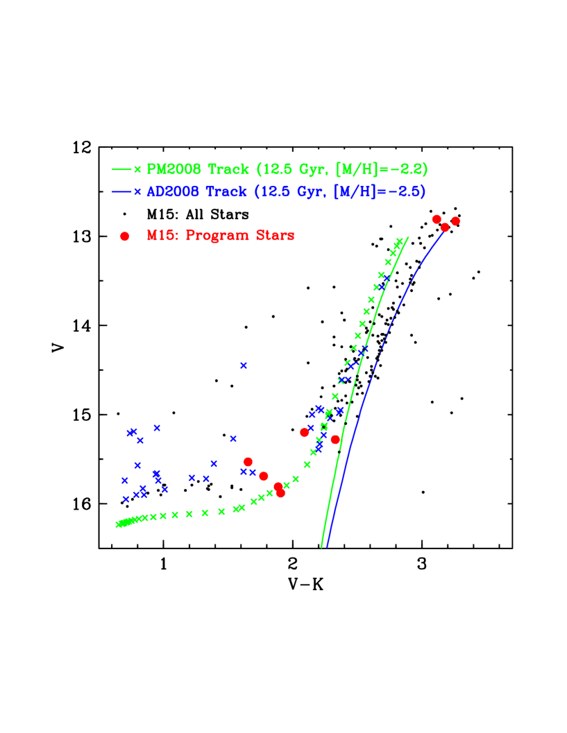
Figure 1: A color-magnitude diagram for the globular cluster M15. For cluster members (indicated by small black dots), $V$ magnitudes are taken Buonanno et al. (1983) while the $K$ magnitudes are obtained from the 2MASS database (Skrutskie et al. 2006). Note that stars with both $B$ and $V$ magnitudes from Buonanno et al. are shown in the plot. The program stars are signified by large, red circles. Also displayed are the isochrone data from both Marigo et al. (2008; labeled PM2008; shown in green) and Dotter et al. (2008; labeled AD2008; shown in blue).

Figure 1 features the color-magnitude diagram (CMD) for the M15 globular cluster with a plot of the $V$ versus $(V-K)$ magnitudes. The $V$ magnitudes for the RGB stars are taken from the prelimiary results of Cudworth (2011) and verified against the data from Cudworth (1976(cud76, )). Alternatively, the RHB $V$ magnitude values are obtained from Buonanno et al. (1983(buo83, )). The $K$ magnitudes for all M15 targets are taken from the Two Micron All Sky Survey (2MASS; Skrutskie et al. 2006(skr06, )). Cluster members with both $B$ and $V$ measurements from Buonanno et al. are displayed in the plot (denoted by the black dots) and the stars of the current study are indicated by large, red circles. Note that the identifications of RGB and RHB members are based upon stellar atmospheric parameters as well as the findings from Sneden et al. (1997(sne97, )) and Preston et al. (2006(pre06, ); please consult those references for additional details). Also in Figure 1, two isochrone determinations are overlayed upon the photometric data: Marigo et al. (2008(mar08, ); with the age parameter set to 12.5 Gyrs and a metallicity of [M/H]=-2.2; shown in green) and Dotter et al. (2008(dot08, ); with the age parameter set to 12.5 Gyrs and a metallicity of [M/H]=-2.5; shown in blue). These are the best-fit isochrones to the general characteristics ascribed to M15 and no preference is given to either source.

Additional observational details of the aforementioned data samples may be found in the original Sneden et al. (1997,2000a)(sne97, ; sne00a, ) and Preston et al. (2006)(pre06, ) publications. These papers also contain descriptions of the data reduction procedures, in which standard IRAF tasks were used for extraction of multi-order wavelength-calibrated spectra from the raw data frames, and specialized software (SPECTRE; Fitzpatrick & Sneden 1987(fit87, )) was employed for continuum normalization and cosmic ray elimination.

Figure 2 features a comparison of the spectra of all M15 targets. Displayed in this plot is a small wavelength interval $4121-4133$ Å, which highlights the important n-capture transitions La II at 4123.22 Å and Eu II at 4129.72 Å. The spectra are arranged in decreasing $T_{\rm eff}$ from the top to the bottom of the figure. As shown, the combined effects of $T_{\rm eff}$ and log g influence the apparent line strength, and accordingly, transitions which are saturated in the RGB spectra completely disappear in the warmer RHB spectra.

3 METHODOLOGY AND MODEL DETERMINATION

Several measures were implemented in order to improve and extend the efforts of Sneden et al. (1997, 2000a)(sne97, ; sne00a, ) and Preston et al. (2006(pre06, )). First, the modification of the line analysis program MOOG was performed to accurately ascertain the relative contributions to the continuum opacity (especially necessary for the bluer wavelength regions and the cool, metal-poor RGB targets). Second, the employment of an alternative grid of models was done to obtain an internally consistent set of stellar atmospheric parameters for the total M15 sample. Third, the utilization of the most up-to-date experimentally and semi-empirically-derived transition probability data was done to determine the abundances from multiple species.

3.1 Atomic Data

Special effort was made to employ the most recent laboratory measurements of oscillator strengths. When applicable, the inclusion of hyperfine and isotopic structure was done for the derivation of abundances. Tables 2 and 3 list the various literature sources for the transition probability data. Some species deserve special comment. The Fe transition probability values are taken from the critical compilation of Fuhr & Wiese (2006(fuh06, ); note for neutral Fe, the authors heavily weigh the laboratory data from O’Brian et al. 1991(obr91, )). No up-to-date laboratory work has been done for Sr, and so, the adopted gf-values are from the semi-empirical study by Brage et al. (1998(bra98, ); these values are in good agreement with those derived empirically by Gratton & Sneden 1994(gra94, )). Similarly, the most recent laboratory effort for Y was by Hannaford et al. (1982(han82, )). Yet these transition probabilities appear to be robust, yielding small line-to-line scatter.

A particular emphasis of the current work is the n-capture element abundances, for which a wealth of new transition probability data have become recently available. Correspondingly, the extensive sets of rare earth $gf$-values from the Wisconsin Atomic Physics Group were adopted (Sneden et al. 2009(sne09, ), Lawler et al. 2009(law09, ), and references therein). These data when applied to the solar spectrum yield photospheric abundances that are in excellent agreement with meteoritic abundances. For neutron capture elements not studied by the Wisconsin group (which include Ba, Pr, Yb, Os, Ir, and Th), alternate literature references were employed (and these are accordingly given in the two aforementioned tables).

3.2 Consideration of Isotropic, Coherent Scattering

In the original version of the line transfer code MOOG (Sneden 1973(sne73, )), local thermodynamic equilibrium (LTE) was assumed and hence, scattering was treated as pure absorption. Accordingly, the source function, $S_{\lambda}$, was set equal to the Planck function, $B_{\lambda}(T)$, which is an adequate assumption for metal-rich stars in all wavelength regions. However for the extremely metal-deficient, cool M15 giants, the dominant source of opacity switches from H^-_BF to Rayleigh scattering in the blue visible and ultraviolet wavelength domain ($\lambda\lesssim 4500$Å). It was then necessary to modify the MOOG program as the LTE approximation was no longer sufficient (this has also been remarked upon by other abundance surveys, e.g. Johnson 2002(joh02, ) and Cayrel et al. 2004(cay04, )).

The classical assumptions of one-dimensionality and plane-parallel geometry continue to be employed in the code. Now with the inclusion of isotropic, coherent scattering, the framework for solution of the radiative transfer equation (RTE) shifts from an initial value to a boundary value problem. The source function then assumes the form of $S=(1-\epsilon)J+\epsilon B$ and the description of line transfer becomes an integro-differential equation. The chosen methodology for the solution of the RTE (and the determination of mean intensity) is the approach of short characteristics that incorporates aspects of an accelerated convergence scheme. In essence, the short characteristics technique employs a tensor product grid in which the interpolation of intensity values occurs at selected grid points. The prescription generally followed was that from Koesterke et al. (2002(koe02, ) and references therein). The Appendix provides more detail with regard to the MOOG program alterations.

Prior to these modifications, for a low temperature and low metallicity star (e.g. a RGB target), the ultraviolet and blue visible spectral transitions reported aberrantly high abundances in comparison to those abundances found from redder lines. With the implementation of the revised code, better line-to-line agreement is found and accordingly, the majority of the abundance trend with wavelength is eliminated for these types of stars. Note for the RHB targets, minimal changes are seen in abundances with the employment of the modified MOOG program (as the dominant source of opacity for these relatively warm stars is always H^-_BF over the spectral region of interest).

3.3 Atmospheric Parameter Determination

To obtain preliminary estimates of $T_{\rm eff}$ and log g for the M15 stars, photometric data from the aforementioned sources (Cudworth 2011; Buonanno et al. 1983(buo83, ); 2MASS) were employed as well as those data from Yanny et al. 1994(yan94, ). To transform the color, the color-$T_{\rm eff}$ relations of Alonso et al. (1999)(alo99, ) were used in conjunction with the distance modulus ($(m-M)_{0}$ = 15.25) and reddening ($E(B-V)$ = 0.10) determinations from Kraft & Ivans (2003(kra03, )). Note that an additional intrinsic uncertainty of about 0.1 dex in log g remains among luminous RGB stars owing to stochastic mass loss of order 0.1 dex. Consequently, initial masses of 0.8 $M_{\odot}$ and 0.6$M_{\odot}$ were assumed for RGB and RHB stars respectively. The photometric V and (V-K) values as well as the photometrically- and spectroscopically-derived stellar atmospheric parameters are collected in Table 1.

With the use of the spectroscopic data analysis program SPECTRE (Fitzpatrick & Sneden 1987(fit87, )), the equivalents widths (EW) of transitions from the elements Ti I/II, Cr I/II, and Fe I/II were measured in the wavelength range 3800-6850 Å. The preliminary $T_{\rm eff}$ values were adjusted to achieve zero slope in plots of Fe abundance (log $(\epsilon_{FeI}$)) as a function of excitation potential ($\chi$) and wavelength ($\lambda$). The initial values of log g were tuned to minimize the disagreement between the neutral and ionized species abundances of Ti, Cr, and Fe (particular attention was paid to the Fe data). Lastly, the microturbulent velocities $v_{\rm t}$ were set as to reduce any dependence on abundance as a function of EW. Final values of $T_{\rm eff}$, log g, $v_{\rm t}$, and metallicity [Fe/H] are listed in Table 1, as well as those values previously derived by Sneden et al. (2000a(sne00a, )) for the RGB stars and Preston et al. (2006)(pre06, ) for the RHB stars.

3.4 Selection of Model Type

To conduct a standard abundance analysis under the fundamental assumptions of one-dimensionality and local thermodynamic equilibrium (LTE), two grids of model atmospheres are generally employed: Kurucz-Castelli (Castelli & Kurucz 2003(cas03, ); Kurucz 2005(kur05, )) and MARCS (Gustafsson et al. 2008(gus08, )). The model selection criteria were as follows: the reconciliation of the metallicity discrepancy between the RGB and RHB stars of M15, the derivation of (spectroscopic-based) atmospheric parameters in reasonable agreement with those found via photometry, and the attainment of ionization balance between the Fe I and Fe II transitions. For the RHB targets, interpolated models from the Kurucz-Castelli and MARCS grids were comparable and yielded extremely similar abundance results. However, there are a few notable differences between the two model types for the RGB stars with regard to the P_gas and P_electron content pressures. Though beyond the scope of the current effort, it would be of considerable interest to examine in detail the exact departures between the Kurucz-Castelli and MARCS grids. To best achieve the aforementioned goals for the M15 data set, MARCS models were accordingly chosen.

3.5 Persistent Metallicity Disagreement between RGB and RHB stars

For the RHB stars, the presently-derived metallicties differ slightly from those of Preston et al. (2006): $<$[Fe_I/H]$>$ = -2.69 (a change of $\Delta=-0.03$) and $<$[Fe_II/H]$>$ = -2.64 (a change of $\Delta=-0.04$). However for the RGB stars, the [Fe/H] results of the current study do vary significantly from those of Sneden et al. (2000): $<$[Fe_I/H]$>$ = -2.56 (a downwards revision of $\Delta=-0.26$) and $<$[Fe_II/H]$>$ = -2.53 (a downwards revision of $\Delta=-0.28$). The remaining metallicity discrepancy between the RGB and RHB stars is as follows: $\Delta(RGB-RHB)_{FeI}$ = 0.13 and $\Delta(RGB-RHB)_{FeII}$ = 0.11. Even with the employment of MARCS models and the incorporation of Rayleigh scattering (not done in previous efforts), the offset persists. Repeated exercises with variations in the $T_{\rm eff}$, log g, and $v_{\rm t}$ values showed that this metallicity disagreement in all likelihood cannot be attributed to differences in these atmospheric parameters. As a further check, the derivation of [Fe_I,II/H] values was performed with a list of transitions satisfactorily measurable in both RGB and RHB spectra. No reduction in the metallicty disagreement was seen as the offsets were found to be: $\Delta(RGB-RHB)_{FeI}$ = 0.11 (with 45 candidate Fe_I lines) and $\Delta(RGB-RHB)_{FeII}$ = 0.14 (with 3 candidate Fe II_II lines).

The data from the M15 RGB and RHB stars originate from different telescope/instrument set-ups. Additionally, somewhat different data reduction procedures were employed for the two samples. Possible contributors to the iron abundance offset could be the lack of consideration of spherical symmetry in the line transfer computations and the generation of sufficiently representative stellar atmospheric models for these highly evolved stars (which exist at the very tip of the giant branch and/or have undergone He-core flash). Indeed, it is difficult to posit a single, clear-cut explanation for the disparity in the RGB and RHB [Fe/H] values. In an analysis of the globular cluster M92, King et al. (1998(kin98, )) derived an average abundance ratio of $<$[Fe/H]$>=$ -2.52 for six subgiant stars, a factor of two lower than the $<$[Fe/H]$>$ value measured in the red giant stars. Similarly, Korn et al. (2007)(kor07, ) surveyed turn off (TO) and RGB stars of NGC 6397 and found a metallicity offset of about 0.15 dex (with the TO stars reporting consistently lower values of [Fe/H]). They argued that the TO stars were afflicted by gravitational settling and other mixing processes and as a result, the Fe abundances of giant stars were likely to be nearer to the true value. While the TO stars do have $T_{\rm eff}$ values close to that of the M15 RHB stars, they have surface gravities and lifetimes that are considerably larger. Accordingly, it is not clear if the offset in M15 has a physical explanation similar to that proposed in the case of NGC 6397.

4 ABUNDANCE RESULTS

For the extraction of abundances, the two filters of line strength and contaminant presence were used to assemble an effective line list. Abundance derivations for the majority of elements employed the technique of synthetic spectrum line profile fitting (accomplished with the updated MOOG code as described in §3.2). For a small group of elements (those whose associated spectral features lack both hyperfine and isotopic structure), the simplified approach of EW measurement was used (completed with both the MOOG code and the SPECTRE program; Fitzpatrick & Sneden 1987(fit87, )). Presented in Tables 2 and 3 are the log $\epsilon$ abundance values for the individual transitions detected in the M15 RGB and RHB stars respectively. These tables also list the relevant line parameters as well as the associated literature references for the $gf$-values employed.

In addition to the line-to-line scatter, errors in the abundance results may arise due to uncertainties in the model atmospheric parameters. To quantify these errors in the M15 data set, a RGB target, K462, is first selected. If alterations of $\Delta T_{eff}=\pm 100$ K are applied, then the abundances of neutral species change by approximately $\Delta$[X_I/H] $\simeq\pm 0.15$ whereas the abundances of singly-ionized species change by about $\Delta$[X_II/H] $\simeq\pm 0.04$. Variations of $\Delta$log g $=\pm 0.20$ yield $\Delta$[X_I/H] $\simeq\pm 0.04$ in neutral species abundances and $\Delta$[X_II/H] $\simeq\pm 0.05$ in singly-ionized species abundances. Changes in the microturbulent velocity on the order of $\Delta$$v_{\rm t}$ $=\pm 0.20$ result in abundance variations of $\Delta$[X_I/H] $\simeq\pm 0.08$ and $\Delta$[X_II/H] $\simeq\pm 0.04$. The exact same procedure is then repeated for the RHB star, B009. Modifications of the temperature by $\Delta T_{eff}=\pm 100$ K lead to abundance changes of $\Delta$[X_I/H] $\simeq\pm 0.09$ in neutral species and $\Delta$[X_II/H] $\simeq\pm 0.02$ in singly-ionized species. Alterations of the surface gravity by $\Delta$log g $=\pm 0.20$ engender variations of $\Delta$[X_I/H] $\simeq\pm 0.01$ and $\Delta$[X_II/H] $\simeq\pm 0.07$. Finally, variations of $\Delta$$v_{\rm t}$ $=\pm 0.20$ produce abundance changes of $\Delta$[X_I/H] $\simeq\pm 0.08$ and $\Delta$[X_II/H] $\simeq\pm 0.04$.

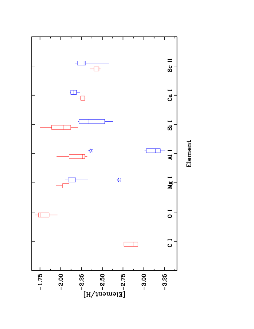
Figure 3: Binned abundances for the elements with $Z=6,8,12-14,20-21$ displayed as quartile boxplots. For each species, the boxplot shows the median, the upper and lower quartiles, and the extremes for both the RGB (denoted in red) and RHB (signified in blue) samples. Outliers, data points with values greater than 1.25 times the median, are indicated by star symbols. Note that there are no RHB points for C I and O I. Note that a depletion in the relative carbon abundance with respect to solar is found.

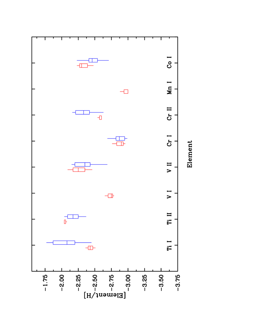
Figure 4: Binned abundances for the elements with $22\leq Z\leq 27$ displayed as quartile boxplots. For each species, the boxplot shows the median, the upper and lower quartiles, and the extremes for both the RGB (denoted in red) and RHB (signified in blue) samples. Note that no RHB data exist for V I. Also, the Mn I results have been set aside for the RHB stars (consult the text for further information). The most consistent agreement between neutral and first-ionized species is found for Ti in all M15 stars.

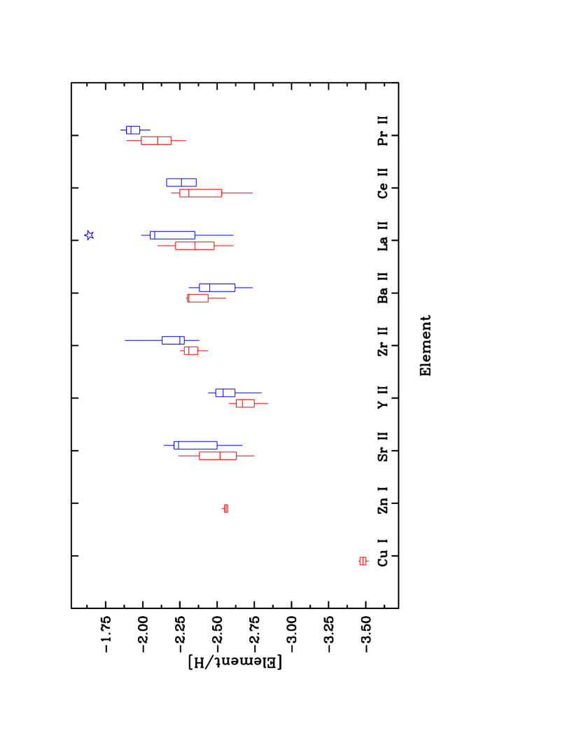
Figure 5: Binned abundances for the elements with $Z=29,30,38-40,56-59$ displayed as quartile boxplots. For each species, the boxplot shows the median, the upper and lower quartiles, and the extremes for both the RGB (denoted in red) and RHB (signified in blue) samples. Outliers, data points with values greater than 1.25 times the median, are indicated by star symbols. Note that there are no RHB data points for Cu I and also, only one RHB abundance value for Zn I.

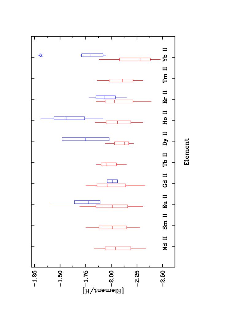
Figure 6: Binned abundances for the elements with $60\leq Z\leq 70$ displayed as quartile boxplots. For each species, the boxplot shows the median, the upper and lower quartiles, and the extremes for both the RGB (denoted in red) and RHB (signified in blue) samples. Outliers, data points with values greater than 1.25 times the median, are indicated by star symbols. Note that only one RHB abundance value was found for the elements Nd II, Sm II, and Tm II. In the case of Tb II, no RHB measurements were possible.

To discuss the abundance results in the following subsections, the elements are divided into four groupings: light ($Z=8$; $11\leq Z\leq 21$; Figure 3), iron-peak ($22\leq Z\leq 28$; Figure 4), light/intermediate n-capture ($29\leq Z\leq 59$; Figure 5), and heavy/other ($60\leq Z\leq 70$; $Z=72,76,77,90$; Figure 6). The measurement of abundances was completed for a total of 40 species. Note that for the elements Sc, Ti, V, and Cr, abundance determinations were possible for both the neutral and first-ionized species. In light of Saha-Boltzmannn calculations for these elements, greater weight is given to the singly-ionized abundances (i.e. for the stars of the M15 data set, only a small fraction of these elements predominantly reside in the neutral state).

Figures 3, 4, 5, and 6 exhibit the abundance ratios for the M15 sample in the form of quartile box plots. These plots show the interquartile range, the median, and the minimum/maximum of the data. Outliers, points which have a value greater than 1.25 times the median, are also indicated. For all of the figures, RGB abundances are signified in red while RHB abundances are denoted in blue. Note that the plots depict the abundance results in the [Elem/H] form in order to preclude erroneous comparisons of the RGB and RHB data, which would arise from the iron abundance offset between the two groups.

Table 4 contains the $<$[Elem/Fe]$>$ values for elements analyzed in the M15 sample along with the line-to-line scatter (given in the form of standard deviations), and the number of lines employed. The subsequent discussion will generally refer to these table data and as is customary, present the relative element abundances with associated $\sigma$ values. The reference solar photospheric abundances (without non-LTE correction) are largely taken from the three-dimensional analyses of Asplund et al. (2005, 2009(asp05a, ; asp09, )) and Grevesse et al. (2010(gre10, )). However, the photospheric values for some of the $n$-capture elements are obtained from other investigations (e.g. Lawler et al. 2009(law09, )). Table 5 lists all of the chosen log $\epsilon_{\sun}$ numbers. Note that in the derivation of the relative element abundance ratios [X/Fe], $<$[Fe_I/H]$>$ are employed for the neutral species transitions while $<$[Fe_II/H]$>$ are used for the singly-ionized lines. This is done in order to minimize ionization equilibrium uncertainties as described in detail by Kraft & Ivans (2003)(kra03, ).

4.1 General Abundance Trends

Within the RGB sample, the neutron capture element abundances of K462 are consistently the largest whereas those of K583 are the smallest. The two RHB stars, B009 and B262, exhibit abundance trends similar to those of the RGB objects. The expected anti-correlations in the proton capture elements (e.g. Na-O and Mg-Al) are seen. The greatest abundance variation with regard to the entire M15 data set is found for the neutron capture elements. Indeed, the star-to-star spread for the majority of n-capture abundances is demonstrable for all M15 targets and is not likely due to internal errors.

Inspection of Table 4 data indicates that RHB stars generally have higher $r$-process element abundances than RGB stars (on average $\Delta$[Elem/Fe]${}_{RHB-RGB}\approx$ 0.3 dex). A sizeable portion of the discrepancy is attributable to the difference in the iron abundances as $<$[Fe/H]$>_{RHB}$ is approximately 0.12 dex lower than $<$[Fe/H]$>_{RGB}$. The remaining offset is most likely a consequence of the small number of targets coupled with a serious selection effect. The original sample of RHB stars from Preston et al. (2006(pre06, )) was chosen as a random set of objects with colors and magnitudes representative of the red end of the HB. These objects were selected without prior knowledge of the heavy element abundances. On the other hand, the three RGB stars from Sneden et al. (2000a(sne00a, )) were particularly chosen as representing the highest and lowest abundances of the $r$-process  as predetermined in the 17 star sample of Sneden et al. (1997(sne97, )).

4.2 Light Element Abundances

The finalized set of light element abundances include: C, O, Mg, Al, Si, Ca, and Sc_I/II. In general, an enhancement of these element abundances relative to solar is seen in the entire M15 data set.

An underabundance of carbon was found in one RHB and three RGB targets of M15 based on the measurement of CH spectral features. As the forbidden O I lines were detectable only in RGB stars, the average abundance ratio for M15 is $<$[O/Fe]$>_{RGB}=+0.75$. This value is substantially larger than that found by Sneden et al. (1997)(sne97, ). A portion of the discrepancy is due to the approximate 0.15 dex difference in the $<$[Fe_I/H]$>$ values between the two investigations. The remainder of departure may be attributed to the adoption of different solar photospheric oxygen values: the current study employs log $\epsilon(O)_{\odot}=8.71$ (Scott et al. 2009(sco09, )) while Sneden et al. uses log $\epsilon(O)_{\odot}=8.93$ (Anders & Grevesse 1989(and89, )).

For the determination of the sodium abundance, the current study relies solely upon the D₁ resonance transitions. Table 4 lists the spuriously large spreads in the Na abundance for both the RGB and RHB groups. The Na D₁ lines are affected by the non-LTE phenomenon of resonance scattering (Asplund 2005b(asp05b, ); Andrievsky et al. 2007(and07, )), which MOOG does not take into account. Also, Sneden et al. (2000b(sne00b, )) made note of the relative strength and line profile distortions associated with these transitions and chose to discard the [Na/Fe] values for stars with $T_{\rm eff}$ $>$ 5000 K. Consequently, the sodium results from the current study are given little weight and are not plotted in Figure 3.

Aluminum is remarkable in its discordance: $<$[Al_I/Fe_I]$>=0.37$ for one RHB and three RGB targets whereas $<$[Al_I/Fe_I]$>=-0.43$ for five RHB stars. Now, the relative aluminum abundances for the RHB stars match well with the values found by Preston et al. (2006(pre06, )). Similarly, the Al abundances from the current analysis agree favorably with the RGB data from Sneden et al. (1997(sne97, )). Though relatively strong transitions are employed in the abundance derivation, the convergence upon two distinct [Al/Fe] values is nontrivial and could merit further exploration.

A decidedly consistent Ca abundance ratio is found for the RGB sample: $<[Ca_{I}/Fe_{I}]>_{RGB}=0.29$; and, also for the RHB sample: $<$[Ca_I/Fe_I]$>_{RHB}=0.53$. After consideration of the iron abundance offset, the RHB stars still report slightly higher calcium abundances than the RGB stars. Overall, a distinct overabundance of Ca relative to solar is present in the M15 cluster. Note that the Sc_I abundance determination was done for only one M15 star (and gives a rather aberrant result compared to the Sc_II abundance data from the other M15 targets).

4.3 Iron Peak Element Abundances

The list of finalized Fe-peak element abundances consists of Ti_I/II, V_I/II, Cr_I/II, Mn, Co, and Ni. Due to RGB spectral crowding issues, derivations of [Ni_I/Fe_I] ratios are performed only for RHB stars.

Achievement of ionization equilibrium did not occur for any of the perspective species: Ti_I/II, V_I/II, or Cr _I/II. In consideration of the entire M15 data set, the best agreement between neutral and singly-ionized species arises for titanium, with all $<$[Ti/Fe]$>$ ratios being supersolar. The V_II relative abundances compare well with one another for the RGB and RHB targets (comparison for V_I is not possible as there are no RHB data for this species). Both of the RGB and RHB $<$[Cr_I/Fe_I]$>$ ratios are underabundant with respect to solar and the neutral chromium values match almost exactly with one another (after accounting for the [Fe/H] offset). On the other hand, the worst agreement is found for Cr_I/II in RHB stars with $\Delta(II-I)=0.47$.

Subsolar values with minimal scatter were found for the $<$[Mn_I/Fe_I]$>$ ratios in both the RGB and RHB stellar groups. However in comparison to RGB stars, manganese appears to be substantially more deficient in RHB targets. The discrepancy may be attributed to both the RGB/RHB iron abundance disparity as well as the employment of the Mn_I resonance transition at 4034.5 Å for the RHB abundance determination. In particular, Sobeck et al. (2011(sob11, )) have demonstrated that the manganese resonance triplet (4030.7, 4033.1, and 4034.5 Å) fails to be a reliable indicator of abundance. Consequently, the RHB abundance results for Mn_I are given little weight and are not plotted in Figure 4.

4.4 Light and Intermediate n-Capture Element Abundances

Finalized abundances for the light and intermediate n-capture elements include Cu, Zn, Sr, Y, Zr, Ba, La, Ce, and Pr. In general, the RGB element abundance ratios are slightly deficient with respect to the RHB values. Also, enhancement with respect to solar is consistently seen in all M15 targets for the elements Ce and Pr.

An extremely underabundant copper abundance relative to solar was found in the RGB stars: $<$[Cu_I/Fe_I]$>_{RGB}=-0.91$. A similar derivation could not take place in the RGB targets as the Cu_I transitions were too weak. A large divergence between RGB and RHB stellar abundances exists for zinc. Detection of the Zn transitions was possible in only one RHB target, which could perhaps account for some of the discrepancy.

For the entire M15 data set, Y_II exhibits lower relative abundance ratios in juxtaposition to both Sr_II and Zr_II. With regard to the three average elemental abundances (of Sr, Y, Zr), moderate departures between the RGB and RHB groups are seen. Also, a large variation in the $<$[Sr_II/Fe_II]$>$ ratio was found for the members of the RGB group.

Though different sets of lines are employed, the RGB and RHB $<$[Ba_II/Fe_II]$>$ ratios are consistent with one another. A portion of the RHB abundance variation is due to the exclusive use of the resonance transitions in the determination (two lowest temperature RHB stars report quite high $\sigma$ values; these strong lines could not be exploited in the RGB analysis). Notably for this element group, the greatest star-to-star abundance scatter was found for lanthanum: $\Delta_{RGB}=0.46$ and $\Delta_{RHB}=0.61$ (excluding the one RHB outlier). The relative cerium abundances also exhibit a wide spread in the RGB sample.

4.5 Heavy n-Capture Element Abundances

The list of finalized $<$[El/Fe]$>$ ratios for the heavy n-capture elements is as follows: Nd, Sm, Eu, Gd, Tb, Dy, Ho, Er, Tm, Yb, Hf, Os, Ir, Pb and Th. All of these element abundance ratios are enriched with regard to the solar values. As shown in Figure 6, a larger abundance spread is found for this group in comparison to the other element groups.

Note that as $T_{\rm eff}$ increases, the strength of the heavy element transitions rapidly decreases and as a consequence, the use of these lines for abundance determinations in the warmest stars becomes unfeasible. It was possible to obtain robust abundances for Nd, Sm, Tb, and Tm in a single RHB target. On the other hand, abundance extractions for the species Os and Ir were done only in RHB stars (measurements of these element transitions were attainable as less spectral crowding occurs in these stars). Nonetheless, minimal line-to-line scatter is seen for the bulk of RGB and RHB n-capture abundances.

A rigorous determination of the europium relative abundance was performed for all M15 stars: $<$[Eu_II/Fe_II]$>_{RGB}=0.53$ and $<$[Eu_II/Fe_II]$>_{RHB}=0.88$. Despite the iron abundance offset, the largest departure between the two stellar groups is found for the element Ho_II. Further, the greatest star-to-star scatter in the heavy n-capture elements is seen for the [Yb_II/Fe_II] ratio: $\Delta_{RGB}=0.55$ and $\Delta_{RHB}=0.58$.

4.6 Comparison with Previous CTG efforts and Otsuki et al. (2006)

These new abundance results are now compared to those from the four prior CTG publications. For the majority of elements, the current data are in accord with the findings of Sneden et al. (1997, 2000a(sne97, ; sne00a, )) and Preston et al. (2006(pre06, )). In this effort, abundance derivations are performed for 13 new species: Sc_I, V_II, Cu_I, Pr_II, Tb_II, Ho_II, Er_II, Tm_II, Yb_II, Hf_II, Os_I, Ir_I, and Pb_II. For elements re-analyzed in the current study, the abundance data have been improved with the use of higher quality atomic data, additional transitions, and a revised version of the MOOG program. A few large discrepancies in the [El/Fe] ratios do occur between the current study and the previous M15 efforts. These departures can be attributed to the employment of different [Fe/H] and solar photospheric values as well as the updated MOOG code. Accordingly, the results from the current analaysis supersede those from the earlier CTG papers.

As in Sneden et al. 1997(sne97, ), the abundance behavior of the proton capture elements appears to be decoupled from that of the neutron capture elements. Notably for M15, significant spread in the abundances was confirmed for both Ba and Eu. The scatter of $\Delta$log$\epsilon(Ba)=0.48$ and $\Delta$log$\epsilon(Eu)=0.90$ from the current effort is in line with that of $\Delta$log$\epsilon(Ba)=0.60$ and $\Delta$log$\epsilon(Eu)=0.73$ from Sneden et al. (1997)(sne97, ).

Comparison of the findings from the current study to those from Otsuki et al. (2006)(ots06, ) has also been done and will be limited to the only star that the two investigations have in common, K462. Due to differences in the $<$[Fe/H]$>$ values, the log $(\epsilon)$ data of the two analyses are compared. The model atmospheric parameters for K462 differ somewhat between the current effort ($T_{\rm eff}$/log g/$v_{\rm t}$ = 4400/0.30/2.00) and Otsuki et al. ($T_{\rm eff}$/log g/$v_{\rm t}$ = 4225/0.50/2.25). However, the agreement in the abundances for the elements Y, Zr, Ba, La and Eu is rather good between the two studies, with the exact differences ranging: $0.01\leq\mid\Delta(Otsuki-Current)\mid\leq 0.16$. The largest disparity occurs for Sr, with both analyses employing the resonance transitions. As mentioned previously, these lines are not the most rigorous probes of abundance.

4.7 General Relationship of Ba, La, and Eu Abundances

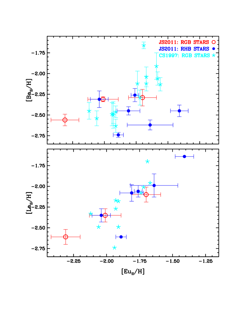
Figure 7: Plots of [(Ba, La)/H] as a function of [Eu/H] for the M15 stars of the current study as well as those from the original Sneden et al. (1997) paper. Also shown are the associated error bars for the abundances (these are the standard deviation values given in Table 4). Note that the Eu and La abundance determinations for the 1997 stellar sample are based upon one transition only (and consequently, no error bars are plotted). Contrary to Sneden et al., no clear evidence of a binary distribution in the abundances is detected.

Sneden et al. (1997)(sne97, ) claimed to have found a binary distribution in a plot of [Ba/Fe] versus [Eu/Fe], with 8 stars exhibiting relative Ba and Eu abundances approximately 0.35 dex smaller than the remainder of the M15 data set. To re-examine their assertion, Figure 7 is generated, which plots [(Ba, La)/H] as a function of [Eu/H] for the entire data sample of the current study. It also displays the re-derived/re-scaled Ba, La, and Eu abundances for all of the giants from the Sneden et al. (1997)(sne97, ) publication. No decisive offset is evident in either panel of Figure 7. For completeness, the equivalent width data from Otsuki et al. (2006)(ots06, ) were also re-analyzed and the abundances were re-determined. Again, no bifurcation was detected in the Ba and Eu data.

5 DATA INTERPRETATION AND ANALYSIS

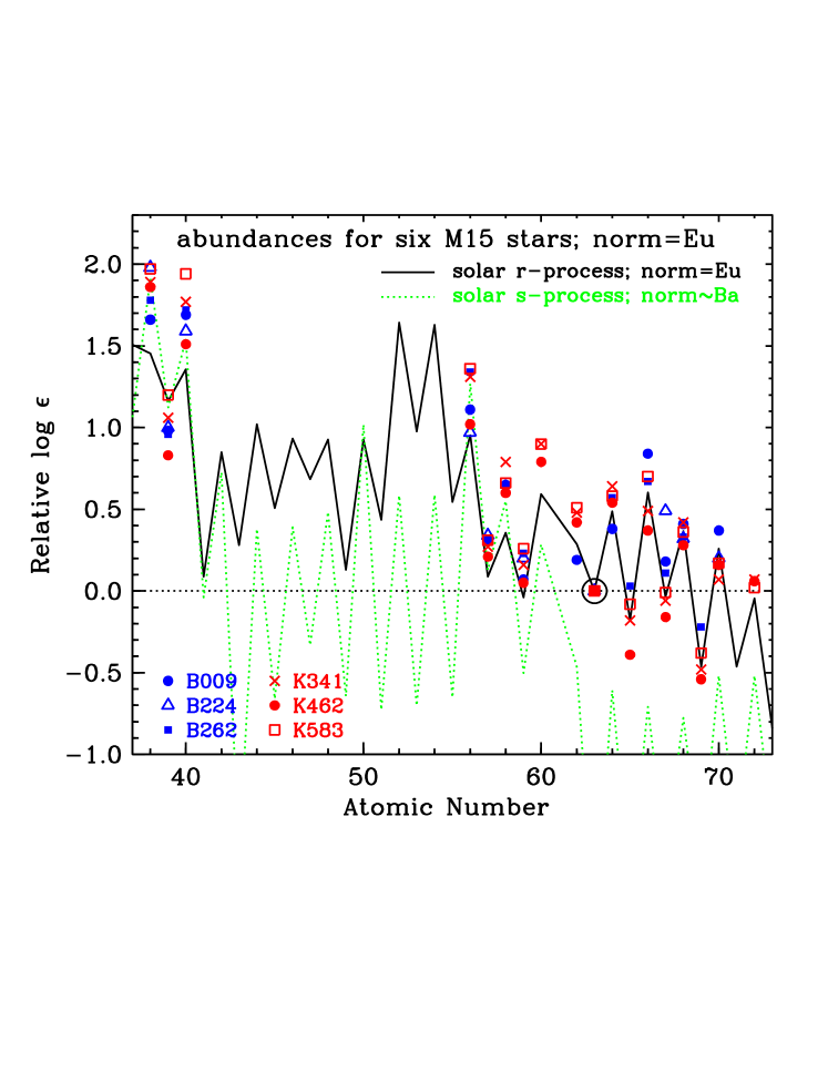
Figure 8: Comparison of the n-capture abundances of six M15 targets to the Solar System r- and s-only abundance distributions. The abundances of the three RGB stars (K341, K462, and K583) are signified by red symbols while the abundances of the three RHB stars (B009, B224, and B262) are designated by blue symbols. The solid black line denotes the $r$-process only abundance pattern, which is scaled to the solar log $\epsilon(Eu)$, and the dotted green line indicates the $s$-process only abundance pattern, which is scaled to the solar log $\epsilon(Ba)$ (all predictions are taken from Sneden, Cowan, & Gallino 2008). The heavy element abundances of the M15 stars compare well to the $r$-process predictions, but not those of the $s$-process. Neither abundance distribution consistently matches the stellar abundances for the elements Sr, Y, and Zr.

A significant amount of $r$-process enrichment has occurred in the M15 globular cluster. Figure 8 plots the average log $\epsilon$ values of the n-capture elements (with $39\leq Z\leq 70$) for three RGB stars (K341, K462, K583; signified by red symbols) and three RHB stars (B009, B224, B262; denoted by blue symbols). The solid black line in this figure indicates the scaled, solar $r$-process prediction as computed by Sneden, Cowan, & Gallino (2008)(sne08, ). All of the element abundances are normalized to the individual stellar log $(\epsilon_{Eu})$ values (Eu is assumed to be an indicator of $r$-process contribution). For the n-capture elements with $Z=64-72$, the RGB stellar abundance values strongly correlate with the solar $r$-process distribution. Similarly for the RHB stars, these abundances match well to the solar $r$-process pattern for most of the elements in the $Z=64-72$ range.

Figure 8 also displays the scaled, solar $s$-process abundance distribution (green, dotted line). The $s$-process predictions are also taken from Sneden, Cowan, & Gallino and the values are normalized to the solar log $(\epsilon_{Ba})$ (Ba is considered to be an indicator of $s$-process contribution). As shown for the $Z=64-72$ elements, there is virtually no agreement between the solar $s$-process pattern and either the RGB or the RHB stellar abundances. The $s$-process predictions compare well to the RGB abundances for only two elements: Ce and La. Thus, it follows that the nucleosynthesis of the heavy neutron capture elements in M15 was dominated by the $r$-process. In addition, the abundance pattern for the light n-capture elements (Sr, Y, Zr) does not adhere to either a solar $r$-process or $s$-process distribution.

5.1 Evidence for Additional Nucleosynthetic Mechanisms Beyond the Classical r- and $s$-process 

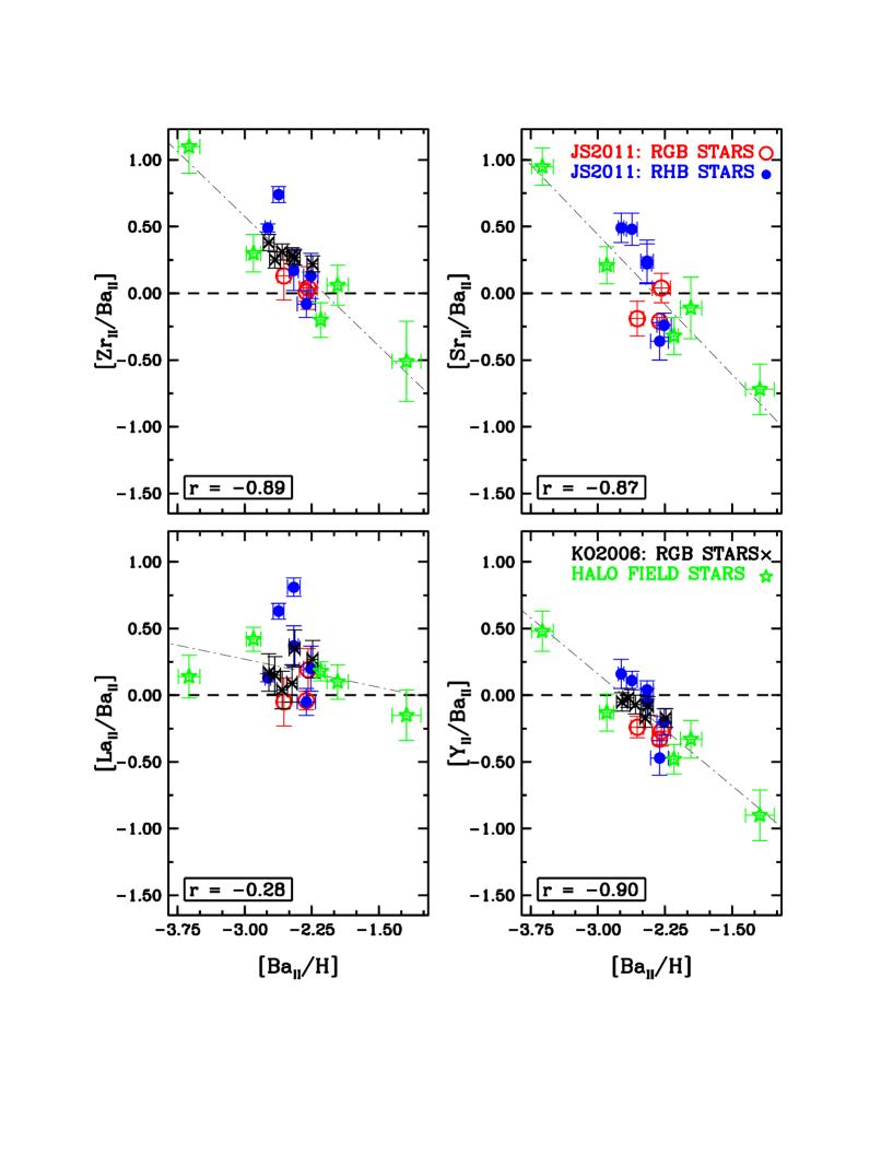
Figure 9: Plot of the relative abundances of the light n-capture elements Sr, Y, and Zr as function of the traditional $s$-process indicator, Ba. All M15 stars from the current effort are shown. Also displayed are the abundance results from Otsuki et al. (2006) as well as those for a few halo field stars (taken from various literature references; see text for further details). The correlation coefficient, r, is exhbited in each of the panels and as seen, Sr, Y , and Zr demonstrate a clear anti-correlative behavior with Ba while La does not.

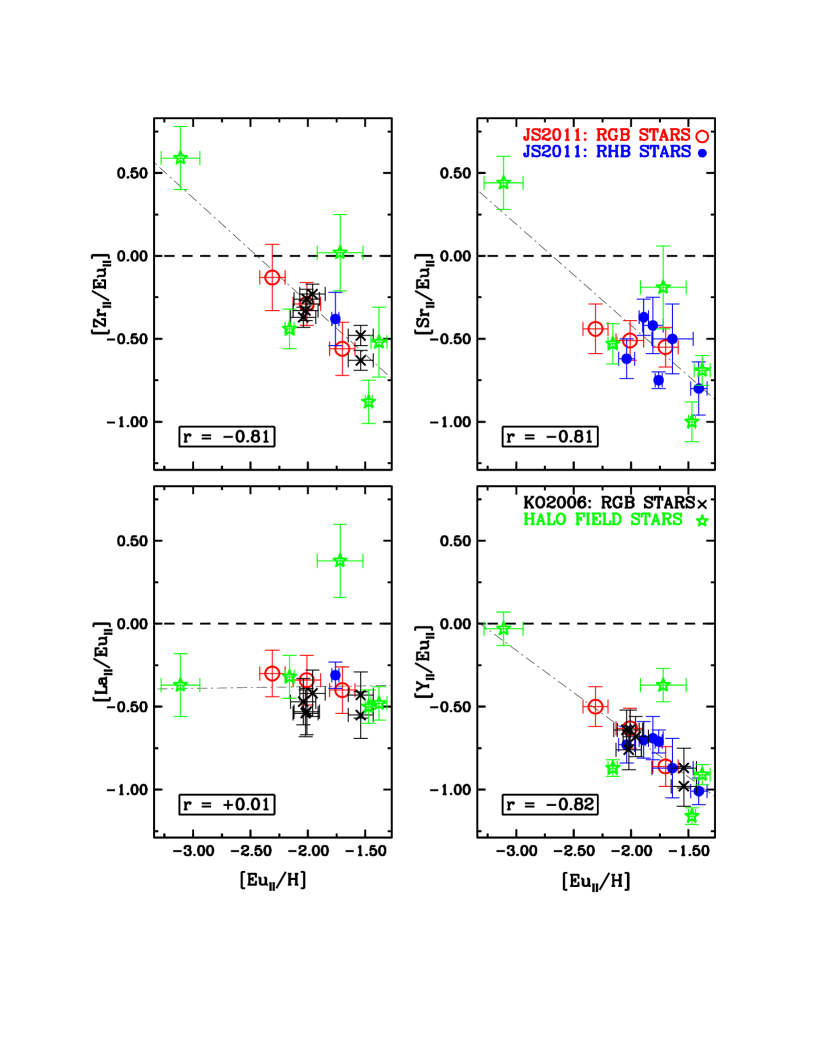
Figure 10: Plot of the relative abundances of the light n-capture elements Sr, Y, and Zr as function of the traditional $r$-process indicator, Eu. All M15 stars from the current effort are shown. Also displayed are the abundance results from Otsuki et al. (2006) as well as those for a few halo field stars (taken from various literature references; see text for further details). The correlation coefficient, r, is exhbited in each of the panels and as seen, Sr, Y , and Zr demonstrate a clear anti-correlative behavior with Eu while La does not.

To further examine the anomalous light n-capture abundances in the M15 cluster, Figures 9 and 10 are generated. For the stars of current effort and those from Otsuki et al. (2006)(ots06, ), these two plots display the abundances of the n-capture elements (Sr, Y, Zr and La) as a function of the [Ba/H] and [Eu/H] ratios, respectively. Moreover, the abundance results from five select field stars which represent extremes in $r$-process or $s$-process enhancement are plotted (CS 22892-052 [Sneden et al. 2003, 2009(sne03, ; sne09, )]; CS 22964-161 [Thompson et al. 2008](tho08, ); HD 115444 [Westin et al. 2000(wes00, ), Sneden et al. 2009(sne09, )]; HD 122563 [Cowan et al. 2005(cow05, ), Lai et al. 2007(lai07, )]; HD 221170 [Ivans et al. 2006(iva06, ), Sneden et al. 2009(sne09, )]).

In Figure 9, an anti-correlative trend is seen for Sr, Y and Zr with Ba while no explicit correlative behavior is apparent for La. The correlation coefficient, $r$, is indicated in each panel. Likewise, La and Eu appear un-correlated in Figure 10. The [(Sr, Y, Zr)/Eu] ratios all exhibit anti-correlation with [Eu/H] in this figure. As shown, the elements Sr, Y, and Zr clearly demonstrate an anti-correlative relationship with both the markers of the $s$-process (Ba) and the $r$-process (Eu).

Figures 9 and 10 collectively imply that the production of the light neutron capture elements most likely did not transpire via the classical forms of the $s$-process or the $r$-process. This finding is not novel. The abundance survey of halo field stars by Travaglio et al. (2004)(tra04, ) previously established the decoupled behavior of the light n-capture species to both Ba and Eu. Further, they postulated that an additional nucleosynthetic process was necessary for the production of these elements (Sr, Y , Zr) in metal-deficient regimes (coined the Lighter Element Primary Process; LEPP).

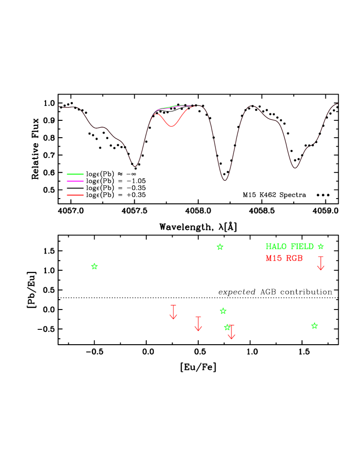
Figure 11: Upper panel: Comparison of synthetic and observed spectra for the Pb I transition at 4057.8 Å in the M15 K462 giant. Four incremental changes in abundance are shown for the specified Pb feature. It is only possible to establish an upper limit of approximately log $\epsilon$ (Pb)$\approx$ -0.35 for this star. A CH contaminant is present in the blue wing of the Pb transition and accounts for a definitive portion of the signal. Accordingly, it appears that the $s$-process element Pb is nominally detected in K462. Lower Panel: Plot of [Pb/Eu] as a function of [Eu/Fe] for three M15 giants and 5 halo field stars. The empirically determined threshold ratio, which indicates the occurrence of AGB enrichment, is shown by the short-dashed line at [Pb/Eu] $\geq+$0.3 (this value is taken from Roederer et al. 2010; see the text for further details). Notice that all of the M15 stars fall below this line (and correspondingly, should lack main $s$-process material).

The overabundances of Sr and Zr (see Figure 8) could have been the result of a small $s$-process contribution to the M15 proto-cluster environment. To investigate this possibility, an abundance determination is performed for Pb, a definitive main $s$-process product. The upper panel of Figure 11 illustrates the synthetic spectrum fits to the neutral Pb transition at a wavelength of 4057.8 Å in the M15 giant, K462. An upper limit of log $\epsilon(Pb)\lesssim$ -0.35 can only be established for this star. For the remaining two RGB targets, upper limits were also determined and accordingly for all three, the average values of log $\epsilon(Pb)\lesssim$ -0.4 and $<$[Pb/Eu]$>$ $\lesssim$ -0.15 were found.

The lower panel of Figure 11 plots [Pb/Eu] as a function of [Eu/Fe] for the three M15 RGB stars and the five, previously-employed halo field stars. In a recent paper, Roederer et al. (2010(roe10, )) suggest that detections of Pb and enhanced [Pb/Eu] ratios should be strong indicators of main $s$-process nucleosynthesis. In turn, they contend that non-detections of Pb and depleted [Pb/Eu] ratios should signify the absence of nucleosynthetic input from the main component of the $s$-process (see their paper for further discussion). With the abundances of 161 low-metallicity stars ([Fe/H] $<$ -1), Roederer et al. empirically determined a threshold value of [Pb/Eu] = +0.3 for minimum AGB contribution. As shown in the figure, the M15 giants lie below this threshold and accordingly, are likely devoid of main $s$-process input. Thus in the case of the M15 globular cluster, the light neutron capture elements presumably originated from an alternate nucleosynthetic process (e.g. $\nu-p$ process, Frohlich et al. 2006(fro06, ); high entropy winds, Farouqi et al. 2009(far09, )).

5.2 M15 Abundances in Relation to the Halo Field

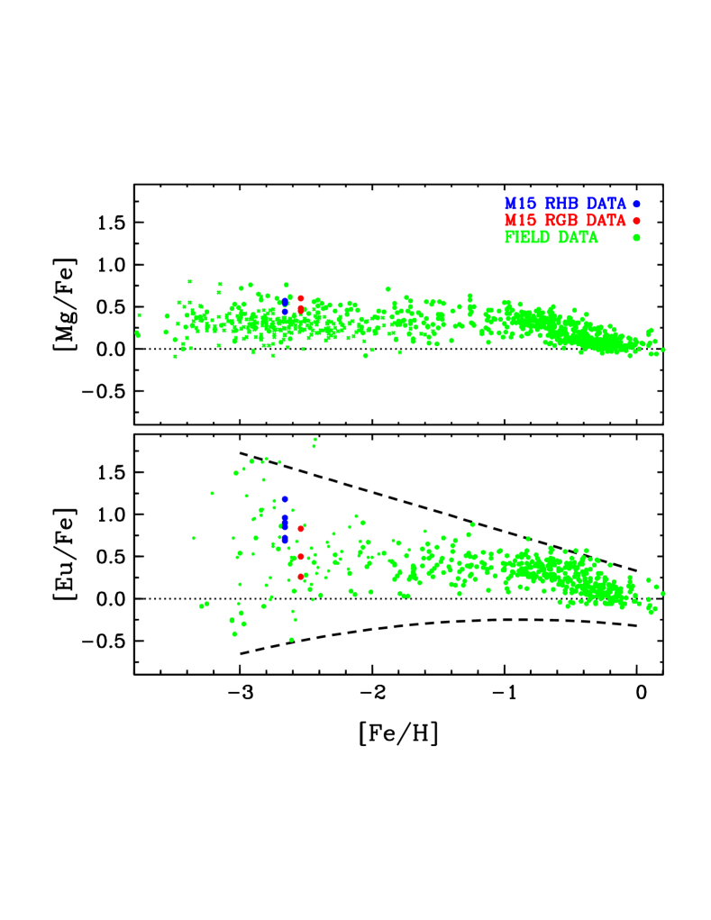
Figure 12: Comparison of the distribution [(Mg, Eu)/Fe] relative abundances as a function of metallicity for M15 targets (denoted by the blue and red circles) as well as for halo and disk stars (signified by the green, filled circles). Field star data have been taken from large sample surveys (see the text for further information). As per convention, the dotted lines represent the Solar abundance ratios. In in the lower panel, the two dashed black lines indicate the approximate ranges of the [Eu/Fe] data. The spread in the [Mg/Fe] values is smaller for M15 than that for the field. Yet for [Eu/Fe], the M15 scatter is comparable to that of the field (for that particular metallicity).

The upper panel of Figure 12 displays the evolution of the [Mg/Fe] abundance ratio with [Fe/H] for all M15 targets as well as for a sample of hundreds of field stars. For this figure, halo and disk star data have been taken from these surveys: Fulbright (2000)(ful00, ), Reddy et al. (2003)(red03, ), Cayrel et al. (2004)(cay04, ), Cohen et al. (2004)(coh04, ), Simmerer et al. (2004)(sim04, ), Barklem et al. (2005)(bar05, ), Reddy, Lambert & Allende Prieto (2006)(red06, ), François et al. (2007)(fra07, ), and Lai et al. (2008)(lai08, ). As shown, the scatter in the [Mg/Fe] abundance ratio is fairly small: $\Delta($[Mg/Fe]$)_{MAX}\approx 0.6$ dex for all stars under conisderation and $\Delta($[Mg/Fe]$)_{MAX}\approx 0.1$ dex for the M15 data set. In the metallicity regime below [Fe/H] $\lesssim$ -1.1, the roughly consistent trend of [Mg/Fe] abundance ratio is due in part to the production history for these elements: magnesium originates from hydrostatic burning in massive stars while iron is manufactured by massive star, core-collapse SNe. If the short evolutionary lifetimes of these massive stars are taken into context with the abundance data, it would seem to indicate that the core-collapse SNe are rather ubiquitous events in the Galactic halo. Accordingly, the products that result from both stellar and explosive nucleosynthesis of massive stars should be well-mixed in the interstellar and intercluster medium. The apparent downward trend in the [Mg/Fe] ratio, in the metallicity region with [Fe/H]$\gtrsim$ -1.1, is due to nucleosynthetic input from Type Ia SNe, which produce much more iron in comparison to Type II events.

In a similar vein, the lower panel of Figure 12 plots [Eu/Fe] as a function of [Fe/H] and demonstrates that as the metallicity decreases, the spread in the [Eu/Fe] abundance ratio increases enormously. By contrast, the scatter in the M15 [Eu/Fe] ratios is large and comparable to the spread of the halo field at that metallicity. Specifically in the metallicity interval -2.7 $\leq$ [Fe/H] $\leq$ -2.2, the scatter in the [Eu/Fe] ratio is found to be $\sigma=\pm 0.27$ for the nine stars of the M15 sample and similarly for the 23 halo giants, the associated scatter is $\sigma=\pm 0.33$. This variation in the relative europium abundance ratio (as first detected by Gilroy et al. 1988(gil88, ) and later confirmed by others, e.g. Burris et al. 2000(bur00, ), Barklem et al. (2005)(bar05, )) indicates an inhomogeneous production history for Eu and other corresponding $r$-process elements. These elements likely originate from lower mass SNe and their production is not correlated with that of the alpha elements (Cowan & Thielemann 2004(cow04, )). Furthermore, it seems that nucleosynthetic events which generated the $r$-process elements were rare occurrences in the early Galaxy. As a consequence, these elements were not well-mixed in the interstellar and intercluster medium (Sneden et al. 2009(sne09, )). Note that $r$-process enhancement seems to be a common feature of all globular clusters (e.g. Gratton, Sneden, & Carretta 2004(gra04, )). On the other hand, the scatter in select $r$-process element abundances, as found in M15, is not.

6 SUMMARY

A novel effort was undertaken to perform a homogenous abundance determination in both the RGB and RHB members of the M15 globular cluster. The current investigation employed improved atomic data, stellar model atmospheres, and radiative transfer code. A resolute offset in the iron abundance between the RGB and RHB stars on the order of 0.1 dex was measured. Notwithstanding, the major findings of the analysis for both the RGB and RHB stellar groups include: a definitive $r$-process enhancement; a significant spread in the abundances of the neutron capture species (which appears to be astrophysical in nature); and, an anti-correlation of light n-capture element abundance behavior with both barium ([Ba/H]) and europium ([Eu/H]). Accordingly, the last set of findings may offer proof of the operation of a LEPP-type mechanism within M15. To determine if these abundance behaviors are generally indicative of very metal-poor globular clusters, a comprehensive examination of the chemical composition of the analogous M92 cluster should be undertaken ([Fe/H] $\sim$ -2.3, Harris et al. 1996(har96, ); the literature contains relatively little information with regard to the n-capture abundances for this cluster).

To date, the presence of multiple stellar generations within the globular cluster M15 has not been irrefutably established. In a series of papers, Carretta et al. (2009a, 2009c, 2010(car09a, ; car09c, ; car10, )) offered compelling proof in the detection of light element anti-correlative behavior (Na-O) in numerous members of the M15 RGB. Lardo et al. (2011(lar11, )) did find a statistically significant spread in the SDSS photometric color index of $u-g$, but yet they were not able to demonstrate a clear and unambiguous correlation of $(u-g)$ with the Na abundances in the RGB of the M15 cluster (which would have provided further evidence). To wit, recent investigations of M15 have revealed several atypical features including: probable detection of an intermediate mass black hole (van der Marel et al. 2002(van02, ); though the result is under some dispute); observation of an intracluster medium (Evans et al. 2003(eva03, )); detection of mass loss (Meszaros et al. 2008, 2009(mez08, ; mez09, )); identification of extreme horizontal branch and blue hook stars (Haurberg et al. 2010(hau10, )); and, observation of an extended tidal tail (Chun et al. 2010(Chun2010, )). It would be worthwhile to examine these peculiar aspects of the globular cluster in relation to the abundance results of M15. Further scrutiny is warranted in order to understand the star formation history and mixing timescale of the M15 protocluster environment.

Appendix A Synopsis

The essential approach to the solution of radiative transfer in the MOOG program has been altered with the employment of short characteristics and the application of an accelerated lambda iteration (ALI) scheme. Original development of the short characteristics (SC) methodology in the context of radiative transfer was done by Mihalas, Auer, & Mihalas (1978(mih78, )). Improvement of the SC approach in the explicit specification of the source function (at all grid points) was made by Olson & Kunasz (1987)(ols87, ) and Kunasz & Auer (1988(kun88, )). As a supplemental reference, the current version of MOOG draws upon the concise treatment of Auer & Paletou (1994(aue94, )). The implementation of the ALI technique within the framework of radiative transfer and stellar atmospheres was first done by Werner (1986(wer86, )) and subsequently refined by both e.g., Rybicki & Hummer (1991(ryb91, )) and Hubeny (1992(hub92, )). The main SC and ALI prescription followed by the MOOG code is that from Koesterke et al. (2002(koe02, ) and references therein). Since the text below is a general description and pertains to the specific coding in MOOG, the reader should consult the aforementioned references as they contain significantly more information.

The primary modification to MOOG is the creation and incorporation of four new subroutines. The names and purposes of the new subroutines are as follows: AngWeight.f, which determines the Gaussian weights and integration points; Sourcefunc_scat_cont.f, which incorporates both a scattering and an absorption component to compute the source function and resultant flux for the continuum; Sourcefunc_scat_line.f, which incorporates both a scattering and an absorption component to compute the source function and resultant flux for the line; and, Cdcalc_JS.f, which calculates the final line depth via the emergent continuum and line fluxes. To accommodate these additions, several key subroutines were also revised. Further details and the publicly-available MOOG code may be found at the website: http://verdi.as.utexas.edu/moog.html. Note that MOOG still retains the capacity to operate in pure absorption mode with the source function set simply to $S=\epsilon B$.

Appendix B Contributions to the Continuous Opacity

To remind the reader, in the visible spectral range, the two principal sources of opacity in stellar atmospheres are the bound-free absorption from the negative hydrogen ion (H^-) and Rayleigh scattering from neutral atomic hydrogen. The standard expression (e.g. Gray 1976(gra76, )) for the H^-_BF absorption coefficient is

$$\kappa\simeq 4.1458\times 10^{-10}\alpha_{BF}P_{e}\Theta^{5/2}10^{0.754\Theta}$$ (B1)

where $\alpha_{BF}$ is the bound-free atomic absorption coefficient (which has frequency dependence), $P_{e}$ is the electron pressure, and $\Theta=5040/T$ (note that Eq. B1 is per neutral hydrogen atom).

With regard to Rayleigh scattering, the scattering cross-section of radiation with angular frequency $\omega$ incident upon a neutral H atom is given by the Kramers-Heisenberg formula in terms of atomic units as

$$\frac{\sigma(\omega)}{\sigma_{T}}=\left(\frac{\omega}{\omega_{1}}\right)^{4}\left|A_{0}+A_{2}\left(\frac{\omega}{\omega_{1}}\right)^{2}+A_{4}\left(\frac{\omega}{\omega_{1}}\right)^{4}+\cdots\right|^{2}$$ (B2)

where $\sigma_{T}$ is the Thompson scattering cross-section and $\omega_{1}$ is the angular frequency corresponding to the Lyman limit. Numerical calculations of the $A_{i}$ coefficients and the generation of an exact expression for Eq. B2 have been done by Dalgarno & Williams (1962(dal62, )) and more recently by Lee & Kim (2004(lee04, )).

The H^-_BF and Rayleigh scattering opacity contributions depend on temperature and metallicity (and to some extent, on the surface gravity). Rayleigh scattering also has a $\lambda^{-4}$ dependence, and as a consequence, it greatly influences blue wavelength transitions. For the majority of stars (such as dwarfs and sub-giants), H^-_BF is the dominant opacity source in the visible spectral regime. However for low temperature, low metallicity giants, the Rayleigh scattering contribution becomes comparable to and even exceeds that from H^-_BF in the ultraviolet and blue visible wavelength regions. Therefore, to accurately determine the line intensity with the correct amount of flux and opacity contribution for all stellar types and over a wide spectral range, isotropic, coherent scattering must be considered.

Appendix C Form of the Radiative Transfer Equation and Implementation of the ALI Scheme

The source function is then written as: $S=(1-\epsilon)J+\epsilon B$ (where $\epsilon$ is the thermal coupling parameter, $J$ is the mean intensity, and $B$ is the Planck function). To commence with the formal solution of the radiation transfer equation, a fundamental assumption is made in that the source function is specified completely in terms of optical depth. After some mathematical manipulation, the radiative transfer equation becomes

$$\mu^{2}\frac{d^{2}j}{d\tau^{2}}=J-S$$ (C1)

where $\mu$ is the directional cosine and $\tau$ is the optical depth. Eq. C1 is an integro-differential equation (and subject to boundary conditions). To obtain the numerical solution of Eq. C1, a discretization in angle and optical depth is necessary. As a consequence, the solution is simplified and a Gaussian quadrature summation is done instead of an integration. Though it is eventually possible to evaluate Eq. C1 in a single step, the use of an iterative method to arrive at a solution is preferred as it is computationally faster than a straightforward approach. For the MOOG program, the ALI technique is employed with the application of a full acceleration. In the context of ALI scheme, the transfer equation takes the form of $J=\Lambda[S]$, where $\Lambda$ represents the matrix operator. Through the concept of preconditioning, ALI allows for the efficient, iterative solution of a (potentially) large system of linear equations. The main steps of the iterative cycle are the evaluation of $J=\Lambda[S]$, the computation of the $\Delta S$ quantity, and the corresponding adjustment to the source function.

Appendix D Short Characteristic Solution of Line Transfer

From a general viewpoint, radiative transfer can be thought of as the propagation of photons along a ray on a two-dimensional grid. Note that the number of rays corresponds to the number of quadrature angles. Determination of radiation along a ray is done periodically at ray segments, or short characteristics. Essentially, SC start at a grid point and proceed along the ray until a cell boundary is met. At these cell boundaries, the intensity, opacity, and source function values are established. Then with the knowledge of the cell boundary intensities, the intensity at other non-grid points can be calculated.

Specifically with regard to MOOG, the intensity determination is a function of depths ($i$) and angles ($j$). It is performed for both an inward ($i-1$) and an outward ($i+1$) direction. Along the characteristic, the opacity quantity is assumed to be a linear function. In effect, the intensity for the ray can be expressed as

$$I=Ie^{-\Delta\tau(i)}+\int S(\tau)e^{-\tau}d\tau$$ (D1)

The optical depth step $\Delta\tau$ can be thought of as the path integral of the opacity along the characteristic (the entire, involved definition of the $\Delta\tau$ quantity is found in the Sourcefunc_scat_* subroutines). Now, the evaluation of Eq. D1 requires the interpolation of the source function. A linear interpolation is sufficient to satisfy the various boundary conditions. Interpolation over [$S(i)$, $S(i\mp 1)$] then entails

$$\int S(\tau)e^{-\tau}d\tau=S(i)w_{1}(i)+S(i\mp 1)w_{2}(i)$$ (D2)

The weights are given by the relations

$$w_{0}(i)=(e^{-\Delta\tau(i)}-1)/\Delta\tau(i)$$ (D3)

$$w_{1}(i)=1+w_{0}(i)$$ (D4)

$$w_{2}(i)=-e^{-\Delta\tau(i)}-w_{0}(i)$$ (D5)

These weights are found by recursion. The use of linear interpolation does not generate significant error (as normally would occur) due to the optically-thin nature of the boundary layer. The expression for the mean intensity, $J$, subsequently becomes

$$J(i)=J(i)+0.5w_{Gau}(j)I$$ (D6)

where the $w_{Gau}$ are the Gaussian quadrature weights (these are distinct from the weights of Eq. D2). The summation over all depth points and angles(/rays) is necessarily performed. The SC formal solution of the transfer equation then proceeds in an iterative manner.

Ongoing and future improvements to the MOOG code include: the incorporation of the Lee & Kim (2004(lee04, )) formulation for Rayleigh scattering (for atomic hydrogen), the employment of a further discretization with regard to frequency, and the implementation of spherically-symmetric geometry in the solution of radiative transfer.

Figure 2: A small wavelength region shown for all program stars. For the purposes of display, the relative fluxes of target stars (other than K341) have been shifted by additive constants. Vertical dotted lines denote the spectral features of La II at a wavelength of 4123.22 Å and of Eu II at 4129.72 Å. Note that these transitions appear to be more pronounced in the spectra of the lower temperature RGB targets.

Table 1: Photometry and Model Atmosphere Parameters

			Current-PHOTO		Current-SPEC				Previous-SPEC
Star	$V$	$V-K$	Teff [K]	$log(g)$	Teff [K]	$log(g)$	[M/H]	vturb [km/s]	Teff [K]	$log(g)$	[M/H]	vturb [km/s]
K341	12.81	3.115	4343	0.88	4375	0.30	-2.25	2.00	4200	0.15	-2.20	2.15
									4225	0.30	-2.20	1.85
K462	12.90	3.178	4298	0.89	4400	0.30	-2.25	2.00	4225	0.15	-2.20	2.10
									4275	0.45	-2.20	2.00
K583	12.83	3.261	4241	0.82	4375	0.30	-2.25	1.90	4275	0.15	-2.20	2.20
									4275	0.30	-2.20	1.90
B009	15.20	2.091	5443	2.26	5300	1.65	-2.50	2.60	5300	1.65	-2.30	2.50
B028	15.88	1.907	5718	2.65	5750	2.40	-2.50	2.85	5750	2.40	-2.50	2.75
B224	15.69	1.775	5932	2.65	5600	2.10	-2.50	2.60	5600	2.10	-2.50	2.60
B262	15.28	2.330	5122	2.16	4950	1.30	-2.50	1.90	5000	1.50	-2.30	1.70
B412	15.81	1.888	5748	2.63	6200	2.70	-2.50	3.30	6250	2.70	-2.50	3.30
B584	15.53	1.655	6142	2.66	6000	2.70	-2.50	2.90	6000	2.70	-2.30	2.70

Table 2: Element Abundances for Individual Transitions in M15 RGB Stars

Element/	Species	Measurement	Wavelength	$\chi$	$log(gf)$	$log\epsilon_{K341}$	$log\epsilon_{K462}$	$log\epsilon_{K583}$	$gf$
Ionization State		Type	[Å]	[eV]					Reference
C I (CH)	6.0	SYNTH	$\approx$ 4300.000	$\cdots$	$\cdots$	5.51	5.76	5.41	Plez & Cohen 2005
O I	8.0	SYNTH	6300.304	0.000	-9.776	7.03	6.88	6.75	Baluja & Zeippen 1988
O I	8.0	SYNTH	6363.776	0.020	-10.257	7.01	7.01	$\cdots$	Baluja & Zeippen 1988
Na I	11.0	EW	5889.950	0.000	0.108	3.45	3.61	4.70	Volz et al. 1996
Na I	11.0	EW	5895.920	0.000	-0.194	$\cdots$	3.42	4.70	Volz et al. 1996
Mg I	12.0	EW	4571.100	0.000	-5.623	5.39	5.42	5.33	Tachiev & Fischer 2003
Mg I	12.0	EW	4702.990	4.346	-0.440	5.65	5.61	5.43	Chang & Tang 1990
Mg I	12.0	EW	5528.400	4.346	-0.498	5.72	5.35	5.48	Chang & Tang 1990
Mg I	12.0	EW	5711.088	4.346	-1.724	$\cdots$	5.34	5.49	Chang & Tang 1990
Al I	13.0	EW	3944.010	0.000	-0.638	4.18	4.23	4.54	Mendoza et al. 1995
Al I	13.0	EW	3961.520	0.010	-0.336	3.93	3.99	4.31	Mendoza et al. 1995
Si I	14.0	EW	3905.523	1.910	-1.041	5.11	$\cdots$	5.42	O’Brian & Lawler 1991
Si I	14.0	EW	4102.936	1.910	-3.336	5.51	5.76	5.61	Fischer 2004
Si I	14.0	EW	5684.484	4.954	-1.420	5.16	$\cdots$	$\cdots$	Nahar & Padhan 1993
Si I	14.0	EW	5690.425	4.930	-1.870	5.43	$\cdots$	5.40	Garz 1973
Ca I	20.0	EW	4425.440	1.879	-0.358	3.91	4.02	3.87	Fuhr & Wiese 1998
Ca I	20.0	EW	5588.760	2.526	0.210	3.94	3.83	3.89	Kostlin 1964
Ca I	20.0	EW	5857.460	2.933	0.230	4.07	3.99	4.06	Kostlin 1964
Ca I	20.0	EW	6102.727	1.879	-0.790	$\cdots$	4.15	3.97	Fuhr & Wiese 1998
Ca I	20.0	EW	6122.230	1.886	-0.315	4.19	4.00	4.03	Fuhr & Wiese 1998
Ca I	20.0	EW	6162.180	1.900	-0.089	4.19	3.93	4.17	Fuhr & Wiese 1998
Ca I	20.0	EW	6439.070	2.526	0.470	$\cdots$	4.02	4.15	Kostlin 1964
Ca I	20.0	EW	6717.690	2.709	-0.524	4.29	4.14	4.13	Fuhr & Wiese 1998

Note. — Table 2 is published in its entirety in the electronic edition of the Astronomical Journal. A portion is shown here for guidance with regard to its form and content.

Table 3: Element Abundances for Individual Transitions in M15 RHB Stars

Element/	Species	Measurement	$\lambda$	$\chi$	$log(gf)$	$log\epsilon_{B009}$	$log\epsilon_{B028}$	$log\epsilon_{B224}$	$log\epsilon_{B262}$	$log\epsilon_{B412}$	$log\epsilon_{B584}$	$gf$
Ionization State		Type	[Å]	[eV]								Reference
Na I	11.0	EW	5889.950	0.000	0.112	5.09	4.05	4.67	4.63	3.81	3.86	Volz et al. 1996
Na I	11.0	EW	5895.920	0.000	-0.191	5.07	3.88	4.54	4.58	3.79	3.75	Volz et al. 1996
Mg I	12.0	EW	3829.360	2.710	-0.227	4.78	5.37	5.35	$\cdots$	$\cdots$	5.38	Tachiev & Fischer 2003
Mg I	12.0	EW	3832.310	2.710	-0.353	4.75	5.42	5.37	5.04	$\cdots$	5.16	Tachiev & Fischer 2003
Mg I	12.0	EW	4571.100	0.000	-5.623	4.90	5.31	5.26	5.19	5.34	5.57	Tachiev & Fischer 2003
Mg I	12.0	EW	5172.684	2.712	-0.393	4.73	5.61	5.44	5.34	5.57	5.52	Tachiev & Fischer 2003
Mg I	12.0	EW	5183.604	2.717	-0.167	4.91	5.62	$\cdots$	5.52	5.76	5.57	Tachiev & Fischer 2003
Mg I	12.0	EW	5528.420	4.346	-0.498	4.92	5.25	5.33	5.14	5.26	5.37	Chang & Tang 1990
Al I	13.0	EW	3944.010	0.000	-0.638	4.09	3.21	3.42	3.50	3.31	3.22	Mendoza et al. 1995
Al I	13.0	EW	3961.530	0.014	-0.336	3.94	3.01	3.30	3.19	3.16	3.13	Mendoza et al. 1995
Si I	14.0	EW	3905.523	1.910	-1.041	$\cdots$	5.11	5.30	5.29	4.98	4.87	O’Brian & Lawler 1991
Si I	14.0	EW	4102.936	1.910	-3.336	5.24	$\cdots$	$\cdots$	$\cdots$	$\cdots$	$\cdots$	Fischer 2004
Ca I	20.0	EW	4226.740	0.000	0.244	4.05	4.29	4.36	3.70	4.29	4.22	Fuhr & Wiese 1998
Ca I	20.0	EW	5588.760	2.526	0.210	4.21	4.02	4.12	3.97	4.18	$\cdots$	Kostlin 1964
Ca I	20.0	EW	5857.460	2.933	0.230	4.25	$\cdots$	4.14	4.24	$\cdots$	$\cdots$	Kostlin 1964
Ca I	20.0	EW	6102.727	1.879	-0.790	4.19	$\cdots$	$\cdots$	3.97	4.27	$\cdots$	Fuhr & Wiese 1998
Ca I	20.0	EW	6122.230	1.886	-0.315	4.22	4.22	4.14	4.12	4.15	$\cdots$	Fuhr & Wiese 1998
Ca I	20.0	EW	6162.180	1.900	-0.089	4.29	4.20	4.08	4.20	4.20	4.13	Fuhr & Wiese 1998
Ca I	20.0	EW	6439.070	2.526	0.470	4.01	4.26	4.01	4.05	4.08	$\cdots$	Kostlin 1964
Ca I	20.0	EW	6493.780	2.521	0.140	3.91	$\cdots$	3.97	$\cdots$	$\cdots$	$\cdots$	Kostlin 1964
Ca I	20.0	EW	6499.650	2.523	-0.590	4.19	$\cdots$	$\cdots$	$\cdots$	$\cdots$	$\cdots$	Kostlin 1964
Ca I	20.0	EW	6717.690	2.709	-0.524	$\cdots$	$\cdots$	$\cdots$	4.24	$\cdots$	$\cdots$	Fuhr & Wiese 1998

Note. — Table 3 is published in its entirety in the electronic edition of the Astronomical Journal. A portion is shown here for guidance with regard to its form and content.

Table 4: Average Relative Abundance Data for M15 Program Stars

	K341	K462	K583	B009	B028	B224	B262	B412	B584
$<$[CI/FeI]$>$	-0.34	-0.08	-0.40	-0.10	$\cdots$	$\cdots$	$\cdots$	$\cdots$	$\cdots$
$\sigma$ (log$\epsilon$(CI))	$\cdots$	$\cdots$	$\cdots$	$\cdots$	$\cdots$	$\cdots$	$\cdots$	$\cdots$	$\cdots$
No. of Lines	1	1	1	1	0	0	0	0	0
$<$[OI/FeI]$>$	0.85	0.78	0.62	$\cdots$	$\cdots$	$\cdots$	$\cdots$	$\cdots$	$\cdots$
$\sigma$ (log$\epsilon$(OI))	0.01	0.09	$\cdots$	$\cdots$	$\cdots$	$\cdots$	$\cdots$	$\cdots$	$\cdots$
No. of Lines	2	2	1	0	0	0	0	0	0
$<$[NaI/FeI]$>$	-0.18	-0.11	1.11	1.60	0.46	1.18	1.21	0.25	0.28
$\sigma$ (log$\epsilon$(NaI))	$\cdots$	0.13	0.00	0.01	0.12	0.09	0.04	0.01	0.08
No. of Lines	1	2	2	2	2	2	2	2	2
$<$[MgI/FeI]$>$	0.60	0.45	0.48	-0.01	0.56	0.56	0.44	0.57	0.54
$\sigma$ (log$\epsilon$(MgI))	0.17	0.13	0.07	0.09	0.15	0.07	0.20	0.23	0.16
No. of Lines	3	4	4	6	2	1	2	2	2
$<$[AlI/FeI]$>$	0.23	0.29	0.64	0.34	-0.60	-0.27	-0.26	-0.52	-0.52
$\sigma$ (log$\epsilon$(AlI))	0.18	0.17	0.16	0.11	0.14	0.08	0.22	0.11	0.06
No. of Lines	2	2	2	2	2	2	2	2	2
$<$[SiI/FeI]$>$	0.33	0.80	0.55	0.42	0.26	0.53	0.55	0.09	0.00
$\sigma$ (log$\epsilon$(SiI))	0.20	0.08	0.01	$\cdots$	$\cdots$	$\cdots$	$\cdots$	$\cdots$	$\cdots$
No. of Lines	4	2	2	1	1	1	1	1	1
$<$[CaI/FeI]$>$	0.33	0.25	0.30	0.53	0.55	0.55	0.54	0.51	0.51
$\sigma$ (log$\epsilon$(CaI))	0.15	0.10	0.12	0.13	0.11	0.13	0.18	0.08	0.06
No. of Lines	6	8	8	9	5	7	9	6	2
$<$[ScI/FeI]$>$	$\cdots$	$\cdots$	-0.76	$\cdots$	$\cdots$	$\cdots$	$\cdots$	$\cdots$	$\cdots$
$\sigma$ (log$\epsilon$(ScI))	$\cdots$	$\cdots$	$\cdots$	$\cdots$	$\cdots$	$\cdots$	$\cdots$	$\cdots$	$\cdots$
No. of Lines	0	0	1	0	0	0	0	0	0
$<$[ScII/FeII]$>$	0.16	0.04	0.12	0.37	0.43	0.37	0.16	0.39	0.32
$\sigma$ (log$\epsilon$(ScII))	0.10	0.12	0.10	0.16	0.06	0.08	0.09	0.20	$\cdots$
No. of Lines	2	2	2	2	3	3	4	2	1
$<$[TiI/FeI]$>$	0.11	0.19	0.07	0.58	0.60	0.54	0.32	0.85	0.77
$\sigma$ (log$\epsilon$(TiI))	0.12	0.13	0.11	0.16	0.16	0.15	0.15	0.08	0.14
No. of Lines	15	12	13	2	4	4	6	2	2
$<$[TiII/FeII]$>$	0.47	0.44	0.47	0.38	0.48	0.40	0.31	0.52	0.50
$\sigma$ (log$\epsilon$(TiII))	0.11	0.13	0.14	0.10	0.10	0.10	0.07	0.07	0.06
No. of Lines	14	8	16	9	7	9	11	8	7
$<$[VI/FeI]$>$	-0.26	-0.11	-0.18	$\cdots$	$\cdots$	$\cdots$	$\cdots$	$\cdots$	$\cdots$
$\sigma$ (log$\epsilon$(VI))	0.07	0.19	0.12	$\cdots$	$\cdots$	$\cdots$	$\cdots$	$\cdots$	$\cdots$
No. of Lines	2	3	3	0	0	0	0	0	0
$<$[VII/FeII]$>$	0.27	0.43	0.11	0.23	0.41	0.31	0.04	$\cdots$	0.44
$\sigma$ (log$\epsilon$(VII))	0.01	0.21	0.21	$\cdots$	0.05	$\cdots$	0.04	$\cdots$	0.03
No. of Lines	2	2	2	1	2	1	2	0	2
$<$[CrI/FeI]$>$	-0.36	-0.22	-0.38	-0.21	-0.24	-0.21	-0.22	-0.07	-0.19
$\sigma$ (log$\epsilon$(CrI))	0.05	0.12	0.07	0.15	0.05	0.12	0.21	0.10	0.09
No. of Lines	5	6	5	4	3	3	8	3	2
$<$[CrII/FeII]$>$	-0.06	-0.02	-0.03	0.33	0.37	0.24	0.10	0.43	0.38
$\sigma$ (log$\epsilon$(CrII))	0.14	0.18	0.06	0.01	0.21	$\cdots$	0.10	0.06	0.07
No. of Lines	4	3	3	2	3	1	3	2	2
$<$[MnI/FeI]$>$	-0.34	-0.45	-0.42	-0.70	-0.74	-0.80	-0.78	$\cdots$	$\cdots$
$\sigma$ (log$\epsilon$(MnI))	0.02	0.04	$\cdots$	$\cdots$	$\cdots$	$\cdots$	$\cdots$	$\cdots$	$\cdots$
No. of Lines	2	2	1	1	1	1	1	0	0
$<$[FeI/H]$>$	-2.53	-2.54	-2.57	-2.69	-2.65	-2.74	-2.77	-2.62	-2.63
$\sigma$ (log$\epsilon$(FeI))	0.14	0.12	0.14	0.12	0.12	0.11	0.14	0.12	0.15
No. of Lines	59	57	63	98	72	72	100	45	60
$<$[FeII/H]$>$	-2.51	-2.51	-2.57	-2.65	-2.60	-2.66	-2.73	-2.59	-2.59
$\sigma$ (log$\epsilon$(FeII))	0.13	0.11	0.10	0.09	0.07	0.13	0.13	0.07	0.13
No. of Lines	8	9	10	12	8	9	11	6	9
$<$[CoI/FeI]$>$	0.07	0.25	0.35	0.45	0.18	0.18	0.04	$\cdots$	0.22
$\sigma$ (log$\epsilon$(CoI))	0.21	0.18	0.20	0.32	$\cdots$	$\cdots$	$\cdots$	$\cdots$	$\cdots$
No. of Lines	2	2	2	2	1	1	1	0	1
$<$[NiI/FeI]$>$	$\cdots$	$\cdots$	$\cdots$	-0.23	$\cdots$	$\cdots$	$\cdots$	$\cdots$	$\cdots$
$\sigma$ (log$\epsilon$(NiI))	$\cdots$	$\cdots$	$\cdots$	0.11	$\cdots$	$\cdots$	$\cdots$	$\cdots$	$\cdots$
No. of Lines	0	0	0	2	0	0	0	0	0
$<$[CuI/FeI]$>$	-0.92	-0.88	-0.92	$\cdots$	$\cdots$	$\cdots$	$\cdots$	$\cdots$	$\cdots$
$\sigma$ (log$\epsilon$(CuI))	$\cdots$	$\cdots$	$\cdots$	$\cdots$	$\cdots$	$\cdots$	$\cdots$	$\cdots$	$\cdots$
No. of Lines	1	1	1	0	0	0	0	0	0
$<$[ZnI/FeI]$>$	0.02	-0.01	0.01	$\cdots$	$\cdots$	0.49	0.27	$\cdots$	$\cdots$
$\sigma$ (log$\epsilon$(ZnI))	0.07	0.07	$\cdots$	$\cdots$	$\cdots$	$\cdots$	0.06	$\cdots$	$\cdots$
No. of Lines	2	2	2	0	0	1	2	0	0
$<$[SrII/FeII]$>$	-0.01	0.28	-0.18	0.16	0.35	0.43	0.06	0.38	0.46
$\sigma$ (log$\epsilon$(SrII))	0.00	0.04	0.11	0.04	0.11	0.14	0.11	0.14	0.11
No. of Lines	2	2	2	2	2	2	2	2	2
$<$[YII/FeII]$>$	-0.13	-0.04	-0.23	0.19	0.02	0.16	-0.04	0.18	0.08
$\sigma$ (log$\epsilon$(YII))	0.04	0.04	0.04	0.06	0.11	0.09	0.09	0.04	0.03
No. of Lines	7	7	6	6	2	4	10	2	3
$<$[ZrII/FeII]$>$	0.21	0.27	0.14	0.53	0.35	0.38	0.35	$\cdots$	0.71
$\sigma$ (log$\epsilon$(ZrII))	0.06	0.12	0.17	0.16	$\cdots$	0.14	0.02	$\cdots$	0.00
No. of Lines	4	4	4	4	1	2	5	0	2
$<$[BaII/FeII]$>$	0.20	0.23	0.01	0.40	-0.14	0.21	0.43	0.14	-0.03
$\sigma$ (log$\epsilon$(BaII))	0.03	0.10	0.07	0.08	0.03	0.05	0.10	0.07	0.06
No. of Lines	4	4	4	5	3	5	6	3	3
$<$[LaII/FeII]$>$	0.16	0.42	-0.04	0.60	-0.01	0.58	0.38		0.60
$\sigma$ (log$\epsilon$(LaII))	0.08	0.09	0.09	0.07	$\cdots$	0.10	0.08	$\cdots$	0.14
No. of Lines	9	9	9	8	1	6	11	1	2
$<$[CeII/FeII]$>$	0.20	0.33	-0.17	0.51	$\cdots$	$\cdots$	0.37	$\cdots$	$\cdots$
$\sigma$ (log$\epsilon$(CeII))	0.15	0.14	0.13	0.13	$\cdots$	$\cdots$	0.14	$\cdots$	$\cdots$
No. of Lines	25	22	11	10	0	0	13	0	0
$<$[PrII/FeII]$>$	0.42	0.63	0.28	0.73	$\cdots$	0.81	0.69	$\cdots$	$\cdots$
$\sigma$ (log$\epsilon$(PrII))	0.04	0.03	0.12	0.00	$\cdots$	$\cdots$	0.11	$\cdots$	$\cdots$
No. of Lines	5	5	5	2	0	1	2	0	0
$<$[NdII/FeII]$>$	0.47	0.68	0.23	0.58	$\cdots$	$\cdots$	$\cdots$	$\cdots$	$\cdots$
$\sigma$ (log$\epsilon$(NdII))	0.10	0.11	0.14	0.10	$\cdots$	$\cdots$	$\cdots$	$\cdots$	$\cdots$
No. of Lines	27	25	22	2	0	0	0	0	0
$<$[SmII/FeII]$>$	0.50	0.77	0.29	0.61	$\cdots$	$\cdots$	$\cdots$	$\cdots$	$\cdots$
$\sigma$ (log$\epsilon$(SmII))	0.08	0.08	0.10	0.13	$\cdots$	$\cdots$	$\cdots$	$\cdots$	$\cdots$
No. of Lines	20	20	15	3	0	0	0	0	0
$<$[EuII/FeII]$>$	0.50	0.83	0.26	0.90	0.72	0.85	0.69	1.18	0.96
$\sigma$ (log$\epsilon$(EuII))	0.12	0.11	0.11	0.03	0.04	0.09	0.07	0.07	0.18
No. of Lines	7	6	7	5	2	5	5	2	2
$<$[GdII/FeII]$>$	0.55	0.77	0.25	0.69	$\cdots$	$\cdots$	0.67	$\cdots$	$\cdots$
$\sigma$ (log$\epsilon$(GdII))	0.08	0.07	0.03	$\cdots$	$\cdots$	$\cdots$	$\cdots$	$\cdots$	$\cdots$
No. of Lines	8	9	3	1	0	0	1	0	0
$<$[TbII/FeII]$>$	0.56	0.67	0.42	$\cdots$	$\cdots$	$\cdots$	0.96	$\cdots$	$\cdots$
$\sigma$ (log$\epsilon$(TbII))	$\cdots$	$\cdots$	$\cdots$	$\cdots$	$\cdots$	$\cdots$	$\cdots$	$\cdots$	$\cdots$
No. of Lines	1	1	1	0	0	0	1	0	0
$<$[DyII/FeII]$>$	0.38	0.58	0.36	1.13	$\cdots$	$\cdots$	0.75	$\cdots$	$\cdots$
$\sigma$ (log$\epsilon$(DyII))	0.15	0.03	0.07	0.08	$\cdots$	$\cdots$	0.11	$\cdots$	$\cdots$
No. of Lines	4	2	4	3	0	0	3	0	0
$<$[HoII/FeII]$>$	0.45	0.67	0.26	1.09	$\cdots$	1.35	0.81	$\cdots$	$\cdots$
$\sigma$ (log$\epsilon$(HoII))	0.05	0.06	0.10	0.10	$\cdots$	$\cdots$	0.05	$\cdots$	$\cdots$
No. of Lines	3	4	3	3	0	1	4	0	0
$<$[ErII/FeII]$>$	0.48	0.67	0.18	0.88	$\cdots$	0.73	0.58	$\cdots$	$\cdots$
$\sigma$ (log$\epsilon$(ErII))	0.15	0.15	0.06	0.03	$\cdots$	0.14	0.05	$\cdots$	$\cdots$
No. of Lines	4	4	3	4	0	2	3	0	0
$<$[TmII/FeII]$>$	0.40	0.66	0.26	$\cdots$	$\cdots$	$\cdots$	0.85	$\cdots$	$\cdots$
$\sigma$ (log$\epsilon$(TmII))	0.09	0.20	0.07	$\cdots$	$\cdots$	$\cdots$	$\cdots$	$\cdots$	$\cdots$
No. of Lines	3	3	2	0	0	0	1	0	0
$<$[YbII/FeII]$>$	0.23	0.64	0.09	0.93	1.29	0.71	$\cdots$	0.89	0.71
$\sigma$ (log$\epsilon$(YbII))	$\cdots$	$\cdots$	$\cdots$	$\cdots$	$\cdots$	$\cdots$	$\cdots$	$\cdots$	$\cdots$
No. of Lines	1	1	1	1	1	1	0	1	1
$<$[HfII/FeII]$>$	0.21	0.52	-0.08	$\cdots$	$\cdots$	$\cdots$	$\cdots$	$\cdots$	$\cdots$
$\sigma$ (log$\epsilon$(HfII))	$\cdots$	$\cdots$	$\cdots$	$\cdots$	$\cdots$	$\cdots$	$\cdots$	$\cdots$	$\cdots$
No. of Lines	1	1	1	0	0	0	0	0	0
$<$[OsI/FeI]$>$	$\cdots$	$\cdots$	$\cdots$	$\cdots$	$\cdots$	$\cdots$	2.00	$\cdots$	$\cdots$
$\sigma$ (log$\epsilon$(OsI))	$\cdots$	$\cdots$	$\cdots$	$\cdots$	$\cdots$	$\cdots$	0.35	$\cdots$	$\cdots$
No. of Lines	0	0	0	0	0	0	2	0	0
$<$[IrI/FeI]$>$	$\cdots$	$\cdots$	$\cdots$	$\cdots$	$\cdots$	$\cdots$	1.35	$\cdots$	$\cdots$
$\sigma$ (log$\epsilon$(IrI))	$\cdots$	$\cdots$	$\cdots$	$\cdots$	$\cdots$	$\cdots$	$\cdots$	$\cdots$	$\cdots$
No. of Lines	0	0	0	0	0	0	1	0	0
$<$[PbI/FeI]$>$	$\lesssim$ 0.44	$\lesssim$ 0.35	$\lesssim$ 0.38	$\cdots$	$\cdots$	$\cdots$	$\cdots$	$\cdots$	$\cdots$
$\sigma$ (log$\epsilon$(PbI))	$\cdots$	$\cdots$	$\cdots$	$\cdots$	$\cdots$	$\cdots$	$\cdots$	$\cdots$	$\cdots$
No. of Lines	1	1	1	0	0	0	0	0	0
$<$[ThII/FeII]$>$	0.46	0.67	0.32	$\cdots$	$\cdots$	$\cdots$	$\cdots$	$\cdots$	$\cdots$
$\sigma$ (log$\epsilon$(ThII))	$\cdots$	$\cdots$	$\cdots$	$\cdots$	$\cdots$	$\cdots$	$\cdots$	$\cdots$	$\cdots$
No. of Lines	1	1	1	0	0	0	0	0	0

Table 5: Solar Photospheric Abundances of the Elements Analyzed in the Current Study

Element	Z	log($\epsilon_{El}$)	Reference	Methodology
H	1	12.00	N/A	$\cdots$
C	6	8.43 $\pm$ 0.05	Asplund et al. 2009	3-D; LTE
O	8	8.71 $\pm$ 0.05	Scott et al. 2009	3-D; LTE
Na	11	6.17 $\pm$ 0.04	Asplund et al. 2005	3-D; LTE
Mg	12	7.53 $\pm$ 0.09	Asplund et al. 2005	3-D; LTE
Al	13	6.37 $\pm$ 0.06	Asplund et al. 2005	3-D; LTE
Si	14	7.51 $\pm$ 0.04	Asplund et al. 2005	3-D; LTE
Ca	20	6.31 $\pm$ 0.04	Asplund et al. 2005	3-D; LTE
Sc	21	3.15 $\pm$ 0.04	Asplund et al. 2009; Grevesse et al. 2010	3-D; LTE
Ti	22	4.95 $\pm$ 0.05	Asplund et al. 2009; Grevesse et al. 2010	3-D; LTE
V	23	3.93 $\pm$ 0.08	Asplund et al. 2009; Grevesse et al. 2010	3-D; LTE
Cr	24	5.64 $\pm$ 0.02	Sobeck et al. 2007	1-D; LTE
Mn	25	5.43 $\pm$ 0.04	Asplund et al. 2009; Grevesse et al. 2010	3-D; LTE
Fe	26	7.52 $\pm$ 0.08	Sneden et al. 1991	1-D; LTE
Co	27	4.99 $\pm$ 0.08	Asplund et al. 2009; Grevesse et al. 2010	3-D; LTE
Ni	28	6.17 $\pm$ 0.02	Scott et al. 2009	3-D; LTE
Cu	29	4.19 $\pm$ 0.04	Asplund et al. 2009; Grevesse et al. 2010	3-D; LTE
Zn	30	4.60 $\pm$ 0.03	Biemont & Godefroid 1980	1-D; LTE
Sr	38	2.92 $\pm$ 0.05	Barklem & O’Mara 2000	1-D; LTE
Y	39	2.21 $\pm$ 0.05	Asplund et al. 2009; Grevesse et al. 2010	3-D; LTE
Zr	40	2.58 $\pm$ 0.04	Asplund et al. 2009; Grevesse et al. 2010	3-D; LTE
Ba	56	2.17 $\pm$ 0.09	Asplund et al. 2009; Grevesse et al. 2010	3-D; LTE
La	57	1.13 $\pm$ 0.03	Lawler et al. 2001	1-D; LTE
Ce	58	1.61 $\pm$ 0.01	Lawler et al.2009	1-D; LTE
Pr	59	0.76 $\pm$ 0.02	Sneden et al. 2009	1-D; LTE
Nd	60	1.45 $\pm$ 0.01	Den Hartog et al. 2003	1-D; LTE
Sm	62	1.00 $\pm$ 0.01	Lawler et al. 2006	1-D; LTE
Eu	63	0.52 $\pm$ 0.01	Lawler et al. 2001	1-D; LTE
Gd	64	1.11 $\pm$ 0.01	Den Hartog et al. 2006	1-D; LTE
Tb	65	0.28 $\pm$ 0.3	Lawler et al. 2001	1-D; LTE
Dy	66	1.13 $\pm$ 0.02	Sneden et al. 2009	1-D; LTE
Ho	67	0.51 $\pm$ 0.10	Lawler et al. 2004	1-D; LTE
Er	68	0.96 $\pm$ 0.03	Lawler et al. 2008	1-D; LTE
Tm	69	0.14 $\pm$ 0.02	Sneden et al. 2009	1-D; LTE
Yb	70	0.86 $\pm$ 0.10	Sneden et al. 2009	1-D; LTE
Hf	72	0.88 $\pm$ 0.08	Lawler et al. 2007	1-D; LTE
Os	76	1.25 $\pm$ 0.11	Quinet et al. 2006	1-D; LTE
Ir	77	1.38 $\pm$ 0.05	Youssef & Khalil 1988	1-D; LTE
Pb	82	1.75 $\pm$ 0.10	Asplund et al. 2009; Grevesse et al. 2010	3-D; LTE
Th	90	0.02 $\pm$ 0.10	Asplund et al. 2009; Grevesse et al. 2010	3-D; LTE

References

- (1) A. Alonso, S. Arribas, and C. Martínez-Roger. A&AS, 140:261–277, December 1999.
- (2) E. Anders and N. Grevesse. Abundances of the elements - Meteoritic and solar. Geochim. Cosmochim. Acta, 53:197–214, January 1989.
- (3) S. M. Andrievsky, M. Spite, S. A. Korotin, F. Spite, P. Bonifacio, R. Cayrel, V. Hill, and P. François. NLTE determination of the sodium abundance in a homogeneous sample of extremely metal-poor stars. A&A, 464:1081–1087, March 2007.
- (4) M. Asplund. New Light on Stellar Abundance Analyses: Departures from LTE and Homogeneity. ARA&A, 43:481–530, September 2005.
- (5) M. Asplund, N. Grevesse, and A. J. Sauval. The Solar Chemical Composition. In T. G. Barnes III & F. N. Bash, editor, Cosmic Abundances as Records of Stellar Evolution and Nucleosynthesis, volume 336 of Astronomical Society of the Pacific Conference Series, pages 25–+, September 2005.
- (6) M. Asplund, N. Grevesse, A. J. Sauval, and P. Scott. The Chemical Composition of the Sun. ARA&A, 47:481–522, September 2009.
- (7) L. H. Auer and F. Paletou. Two-dimensional radiative transfer with partial frequency redistribution I. General method. A&A, 285:675–686, May 1994.
- (8) P. S. Barklem, N. Christlieb, T. C. Beers, V. Hill, M. S. Bessell, J. Holmberg, B. Marsteller, S. Rossi, F.-J. Zickgraf, and D. Reimers. The Hamburg/ESO R-process enhanced star survey (HERES). II. Spectroscopic analysis of the survey sample. A&A, 439:129–151, August 2005.
- (9) L. R. Bedin, G. Piotto, J. Anderson, S. Cassisi, I. R. King, Y. Momany, and G. Carraro. Centauri: The Population Puzzle Goes Deeper. ApJ, 605:L125–L128, April 2004.
- (10) K. Bekki, S. W. Campbell, J. C. Lattanzio, and J. E. Norris. Origin of abundance inhomogeneity in globular clusters. MNRAS, 377:335–351, May 2007.
- (11) R. Bernstein, S. A. Shectman, S. M. Gunnels, S. Mochnacki, and A. E. Athey. MIKE: A Double Echelle Spectrograph for the Magellan Telescopes at Las Campanas Observatory. In M. Iye & A. F. M. Moorwood, editor, Society of Photo-Optical Instrumentation Engineers (SPIE) Conference Series, volume 4841 of Society of Photo-Optical Instrumentation Engineers (SPIE) Conference Series, pages 1694–1704, March 2003.
- (12) T. Brage, G. M. Wahlgren, S. G. Johansson, D. S. Leckrone, and C. R. Proffitt. Theoretical Oscillator Strengths for SR II and Y iii, with Application to Abundances in the HgMn-Type Star chi LUPI. ApJ, 496:1051–+, March 1998.
- (13) R. Buonanno, G. Buscema, C. E. Corsi, G. Iannicola, and F. Fusi Pecci. Positions, magnitudes, and colors for stars in the globular cluster M15. A&AS, 51:83–92, January 1983.
- (14) D. L. Burris, C. A. Pilachowski, T. E. Armandroff, C. Sneden, J. J. Cowan, and H. Roe. Neutron-Capture Elements in the Early Galaxy: Insights from a Large Sample of Metal-poor Giants. ApJ, 544:302–319, November 2000.
- (15) E. Carretta, A. Bragaglia, R. Gratton, V. D’Orazi, and S. Lucatello. Intrinsic iron spread and a new metallicity scale for globular clusters. A&A, 508:695–706, December 2009.
- (16) E. Carretta, A. Bragaglia, R. Gratton, and S. Lucatello. Na-O anticorrelation and HB. VIII. Proton-capture elements and metallicities in 17 globular clusters from UVES spectra. A&A, 505:139–155, October 2009.
- (17) E. Carretta, A. Bragaglia, R. Gratton, S. Lucatello, M. Bellazzini, and V. D’Orazi. Calcium and Light-elements Abundance Variations from High-resolution Spectroscopy in Globular Clusters. ApJ, 712:L21–L25, March 2010.
- (18) E. Carretta, A. Bragaglia, R. G. Gratton, S. Lucatello, G. Catanzaro, F. Leone, M. Bellazzini, R. Claudi, V. D’Orazi, Y. Momany, S. Ortolani, E. Pancino, G. Piotto, A. Recio-Blanco, and E. Sabbi. Na-O anticorrelation and HB. VII. The chemical composition of first and second-generation stars in 15 globular clusters from GIRAFFE spectra. A&A, 505:117–138, October 2009.
- (19) F. Castelli and R. L. Kurucz. New Grids of ATLAS9 Model Atmospheres. In N. Piskunov, W. W. Weiss, & D. F. Gray, editor, Modelling of Stellar Atmospheres, volume 210 of IAU Symposium, pages 20P–+, 2003.
- (20) R. Cayrel, E. Depagne, M. Spite, V. Hill, F. Spite, P. François, B. Plez, T. Beers, F. Primas, J. Andersen, B. Barbuy, P. Bonifacio, P. Molaro, and B. Nordström. First stars V - Abundance patterns from C to Zn and supernova yields in the early Galaxy. A&A, 416:1117–1138, March 2004.
- (21) S.-H. Chun, J.-W. Kim, S. T. Sohn, J.-H. Park, W. Han, H.-I. Kim, Y.-W. Lee, M. G. Lee, S.-G. Lee, and Y.-J. Sohn. A Wide-Field Photometric Survey for Extratidal Tails Around Five Metal-Poor Globular Clusters in the Galactic Halo. AJ, 139:606–625, February 2010.
- (22) J. G. Cohen, N. Christlieb, A. McWilliam, S. Shectman, I. Thompson, G. J. Wasserburg, I. Ivans, M. Dehn, T. Karlsson, and J. Melendez. Abundances In Very Metal-Poor Dwarf Stars. ApJ, 612:1107–1135, September 2004.
- (23) J. J. Cowan, C. Sneden, T. C. Beers, J. E. Lawler, J. Simmerer, J. W. Truran, F. Primas, J. Collier, and S. Burles. Hubble Space Telescope Observations of Heavy Elements in Metal-Poor Galactic Halo Stars. ApJ, 627:238–250, July 2005.
- (24) J. J. Cowan and F.-K. Thielemann. R-Process Nucleosynthesis in Supernovae. Physics Today, 57(10):100000–53, October 2004.
- (25) K. M. Cudworth. Membership and internal motions in the globular cluster M15. AJ, 81:519–526, July 1976.
- (26) A. Dalgarno and D. A. Williams. Rayleigh Scattering by Molecular Hydrogen. ApJ, 136:690–692, September 1962.
- (27) A. Dotter, B. Chaboyer, D. Jevremović, V. Kostov, E. Baron, and J. W. Ferguson. The Dartmouth Stellar Evolution Database. ApJS, 178:89–101, September 2008.
- (28) A. Evans, M. Stickel, J. T. van Loon, S. P. S. Eyres, M. E. L. Hopwood, and A. J. Penny. Far infra-red emission from NGC 7078: First detection of intra-cluster dust in a globular cluster. A&A, 408:L9–L12, September 2003.
- (29) K. Farouqi, K.-L. Kratz, L. I. Mashonkina, B. Pfeiffer, J. J. Cowan, F.-K. Thielemann, and J. W. Truran. Nucleosynthesis Modes in The High-Entropy Wind of Type II Supernovae: Comparison of Calculations With Halo-Star Observations. ApJ, 694:L49–L53, March 2009.
- (30) M. J. Fitzpatrick and C. Sneden. A Software Package for Microcomputer Reductions of Spectroscopic Data. In Bulletin of the American Astronomical Society, volume 19 of Bulletin of the American Astronomical Society, pages 1129–+, September 1987.
- (31) P. François, E. Depagne, V. Hill, M. Spite, F. Spite, B. Plez, T. C. Beers, J. Andersen, G. James, B. Barbuy, R. Cayrel, P. Bonifacio, P. Molaro, B. Nordström, and F. Primas. First stars. VIII. Enrichment of the neutron-capture elements in the early Galaxy. A&A, 476:935–950, December 2007.
- (32) C. Fröhlich, G. Martínez-Pinedo, M. Liebendörfer, F.-K. Thielemann, E. Bravo, W. R. Hix, K. Langanke, and N. T. Zinner. Physical Review Letters, 96(14):142502–+, April 2006.
- (33) J. R. Fuhr and W. L. Wiese. A Critical Compilation of Atomic Transition Probabilities for Neutral and Singly Ionized Iron. Journal of Physical and Chemical Reference Data, 35:1669–1809, December 2006.
- (34) J. P. Fulbright. Abundances and Kinematics of Field Halo and Disk Stars. I. Observational Data and Abundance Analysis. AJ, 120:1841–1852, October 2000.
- (35) K. K. Gilroy, C. Sneden, C. A. Pilachowski, and J. J. Cowan. Abundances of neutron capture elements in Population II stars. ApJ, 327:298–320, April 1988.
- (36) R. Gratton, C. Sneden, and E. Carretta. Abundance Variations Within Globular Clusters. ARA&A, 42:385–440, September 2004.
- (37) R. G. Gratton and C. Sneden. Abundances of neutron-capture elements in metal-poor stars. A&A, 287:927–946, July 1994.
- (38) D. F. Gray. The observation and analysis of stellar photospheres. 1976.
- (39) N. Grevesse, M. Asplund, A. J. Sauval, and P. Scott. The chemical composition of the Sun. Ap&SS, 328:179–183, July 2010.
- (40) P. Guhathakurta, B. Yanny, J. N. Bahcall, and D. P. Schneider. Globular cluster photometry with the Hubble Space Telescope. 3: Blue stragglers and variable stars in the core of M3. AJ, 108:1786–1809, November 1994.
- (41) B. Gustafsson, B. Edvardsson, K. Eriksson, U. G. Jørgensen, Å. Nordlund, and B. Plez. A grid of MARCS model atmospheres for late-type stars. I. Methods and general properties. A&A, 486:951–970, August 2008.
- (42) S.-I. Han, Y.-W. Lee, S.-J. Joo, S. T. Sohn, S.-J. Yoon, H.-S. Kim, and J.-W. Lee. The Presence of Two Distinct Red Giant Branches in the Globular Cluster NGC 1851. ApJ, 707:L190–L194, December 2009.
- (43) P. Hannaford, R. M. Lowe, N. Grevesse, E. Biemont, and W. Whaling. Oscillator strengths for Y I and Y II and the solar abundance of yttrium. ApJ, 261:736–746, November 1982.
- (44) W. E. Harris. A Catalog of Parameters for Globular Clusters in the Milky Way. AJ, 112:1487–+, October 1996.
- (45) N. C. Haurberg, G. M. G. Lubell, H. N. Cohn, P. M. Lugger, J. Anderson, A. M. Cool, and A. M. Serenelli. Ultraviolet-bright Stellar Populations and Their Evolutionary Implications in the Collapsed-core Cluster M15. ApJ, 722:158–177, October 2010.
- (46) H. L. Helfer, G. Wallerstein, and J. L. Greenstein. Abundances in Some Population II K Giants. ApJ, 129:700–+, May 1959.
- (47) S. Honda, W. Aoki, Y. Ishimaru, S. Wanajo, and S. G. Ryan. Neutron-Capture Elements in the Very Metal Poor Star HD 122563. ApJ, 643:1180–1189, June 2006.
- (48) I. Hubeny. Accelerated Lambda iteration (review). In U. Heber & C. S. Jeffery, editor, The Atmospheres of Early-Type Stars, volume 401 of Lecture Notes in Physics, Berlin Springer Verlag, pages 377–+, 1992.
- (49) I. I. Ivans, J. Simmerer, C. Sneden, J. E. Lawler, J. J. Cowan, R. Gallino, and S. Bisterzo. Near-Ultraviolet Observations of HD 221170: New Insights into the Nature of r-Process-rich Stars. ApJ, 645:613–633, July 2006.
- (50) J. A. Johnson. Abundances of 30 Elements in 23 Metal-Poor Stars. ApJS, 139:219–247, March 2002.
- (51) J. R. King, A. Stephens, A. M. Boesgaard, and C. Deliyannis. Keck HIRES spectroscopy of M92 subgiants - Surprising abundances near the turnoff. AJ, 115:666–+, February 1998.
- (52) L. Koesterke, W.-R. Hamann, and G. Gräfener. Expanding atmospheres in non-LTE:. Radiation transfer using short characteristics. A&A, 384:562–567, March 2002.
- (53) A. J. Korn, F. Grundahl, O. Richard, L. Mashonkina, P. S. Barklem, R. Collet, B. Gustafsson, and N. Piskunov. Atomic Diffusion and Mixing in Old Stars. I. Very Large Telescope FLAMES-UVES Observations of Stars in NGC 6397. ApJ, 671:402–419, December 2007.
- (54) R. P. Kraft and I. I. Ivans. A Globular Cluster Metallicity Scale Based on the Abundance of Fe II. PASP, 115:143–169, February 2003.
- (55) K.-L. Kratz, K. Farouqi, B. Pfeiffer, J. W. Truran, C. Sneden, and J. J. Cowan. Explorations of the r-Processes: Comparisons between Calculations and Observations of Low-Metallicity Stars. ApJ, 662:39–52, June 2007.
- (56) P. Kunasz and L. H. Auer. Short characteristic integration of radiative transfer problems - Formal solution in two-dimensional slabs. J. Quant. Spec. Radiat. Transf., 39:67–79, January 1988.
- (57) R. L. Kurucz. ATLAS12, SYNTHE, ATLAS9, WIDTH9, et cetera. Memorie della Societa Astronomica Italiana Supplementi, 8:14–+, 2005.
- (58) H. Küstner. Der entstellende Einfluß des Spektrometerkristalls auf das kontinuierliche Röntgenspektrum. Zeitschrift fur Physik, 7:97–110, December 1921.
- (59) D. K. Lai, M. Bolte, J. A. Johnson, S. Lucatello, A. Heger, and S. E. Woosley. Detailed Abundances for 28 Metal-poor Stars: Stellar Relics in the Milky Way. ApJ, 681:1524–1556, July 2008.
- (60) D. K. Lai, J. A. Johnson, M. Bolte, and S. Lucatello. Carbon and Strontium Abundances of Metal-poor Stars. ApJ, 667:1185–1195, October 2007.
- (61) C. Lardo, M. Bellazzini, E. Pancino, E. Carretta, A. Bragaglia, and E. Dalessandro. Mining SDSS in search of multiple populations in globular clusters. A&A, 525:A114+, January 2011.
- (62) J. E. Lawler, C. Sneden, J. J. Cowan, I. I. Ivans, and E. A. Den Hartog. Improved Laboratory Transition Probabilities for Ce II, Application to the Cerium Abundances of the Sun and Five r-Process-Rich, Metal-Poor Stars, and Rare Earth Lab Data Summary. ApJS, 182:51–79, May 2009.
- (63) H.-W. Lee and H. I. Kim. Rayleigh scattering cross-section redward of Ly by atomic hydrogen. MNRAS, 347:802–806, January 2004.
- (64) P. Marigo, L. Girardi, A. Bressan, M. A. T. Groenewegen, L. Silva, and G. L. Granato. Evolution of asymptotic giant branch stars. II. Optical to far-infrared isochrones with improved TP-AGB models. A&A, 482:883–905, May 2008.
- (65) A. F. Marino, A. P. Milone, G. Piotto, S. Villanova, L. R. Bedin, A. Bellini, and A. Renzini. A double stellar generation in the globular cluster NGC 6656 (M 22). Two stellar groups with different iron and s-process element abundances. A&A, 505:1099–1113, October 2009.
- (66) S. Mészáros, E. H. Avrett, and A. K. Dupree. Mass Outflow from Red Giant Stars in M13, M15, and M92. AJ, 138:615–624, August 2009.
- (67) S. Meszaros, A. K. Dupree, and A. Szentgyorgyi. Mass Outflow and Chromospheric Activity of Red Giant Stars in Globular Clusters.I. M15. AJ, 135:1117–1135, April 2008.
- (68) D. Mihalas, L. H. Auer, and B. R. Mihalas. Two-dimensional radiative transfer. I - Planar geometry. ApJ, 220:1001–1023, March 1978.
- (69) T. R. O’Brian, M. E. Wickliffe, J. E. Lawler, W. Whaling, and J. W. Brault. Lifetimes, transition probabilities, and level energies in Fe i. Journal of the Optical Society of America B Optical Physics, 8:1185–1201, 1991.
- (70) G. L. Olson and P. B. Kunasz. Short characteristic solution of the non-LTE transfer problem by operator perturbation. I. The one-dimensional planar slab. J. Quant. Spec. Radiat. Transf., 38:325–336, 1987.
- (71) K. Otsuki, S. Honda, W. Aoki, T. Kajino, and G. J. Mathews. Neutron-Capture Elements in the Metal-poor Globular Cluster M15. ApJ, 641:L117–L120, April 2006.
- (72) G. Piotto, L. R. Bedin, J. Anderson, I. R. King, S. Cassisi, A. P. Milone, S. Villanova, A. Pietrinferni, and A. Renzini. A Triple Main Sequence in the Globular Cluster NGC 2808. ApJ, 661:L53–L56, May 2007.
- (73) G. W. Preston, C. Sneden, I. B. Thompson, S. A. Shectman, and G. S. Burley. Atmospheres, Chemical Compositions, and Evolutionary Histories of Very Metal-Poor Red Horizontal-Branch Stars in the Galactic Field and in NGC 7078 (M15). AJ, 132:85–110, July 2006.
- (74) Y.-Z. Qian and G. J. Wasserburg. Determination of Nucleosynthetic Yields of Supernovae and Very Massive Stars from Abundances in Metal-Poor Stars. ApJ, 567:515–531, March 2002.
- (75) B. E. Reddy, D. L. Lambert, and C. Allende Prieto. Elemental abundance survey of the Galactic thick disc. MNRAS, 367:1329–1366, April 2006.
- (76) B. E. Reddy, J. Tomkin, D. L. Lambert, and C. Allende Prieto. The chemical compositions of Galactic disc F and G dwarfs. MNRAS, 340:304–340, March 2003.
- (77) I. U. Roederer, J. J. Cowan, A. I. Karakas, K.-L. Kratz, M. Lugaro, J. Simmerer, K. Farouqi, and C. Sneden. The Ubiquity of the Rapid Neutron-capture Process. ApJ, 724:975–993, December 2010.
- (78) G. B. Rybicki and D. G. Hummer. An accelerated lambda iteration method for multilevel radiative transfer. I - Non-overlapping lines with background continuum. A&A, 245:171–181, May 1991.
- (79) P. Scott, M. Asplund, N. Grevesse, and A. J. Sauval. On the Solar Nickel and Oxygen Abundances. ApJ, 691:L119–L122, February 2009.
- (80) J. Simmerer, C. Sneden, J. J. Cowan, J. Collier, V. M. Woolf, and J. E. Lawler. The Rise of the s-Process in the Galaxy. ApJ, 617:1091–1114, December 2004.
- (81) M. F. Skrutskie, R. M. Cutri, R. Stiening, M. D. Weinberg, S. Schneider, J. M. Carpenter, C. Beichman, R. Capps, T. Chester, J. Elias, J. Huchra, J. Liebert, C. Lonsdale, D. G. Monet, S. Price, P. Seitzer, T. Jarrett, J. D. Kirkpatrick, J. E. Gizis, E. Howard, T. Evans, J. Fowler, L. Fullmer, R. Hurt, R. Light, E. L. Kopan, K. A. Marsh, H. L. McCallon, R. Tam, S. Van Dyk, and S. Wheelock. The Two Micron All Sky Survey (2MASS). AJ, 131:1163–1183, February 2006.
- (82) C. Sneden. The nitrogen abundance of the very metal-poor star HD 122563. ApJ, 184:839–849, September 1973.
- (83) C. Sneden, J. J. Cowan, and R. Gallino. Neutron-Capture Elements in the Early Galaxy. ARA&A, 46:241–288, September 2008.
- (84) C. Sneden, J. J. Cowan, J. E. Lawler, I. I. Ivans, S. Burles, T. C. Beers, F. Primas, V. Hill, J. W. Truran, G. M. Fuller, B. Pfeiffer, and K.-L. Kratz. The Extremely Metal-poor, Neutron Capture-rich Star CS 22892-052: A Comprehensive Abundance Analysis. ApJ, 591:936–953, July 2003.
- (85) C. Sneden, J. Johnson, R. P. Kraft, G. H. Smith, J. J. Cowan, and M. S. Bolte. Neutron-Capture Element Abundances in the Globular Cluster M15. ApJ, 536:L85–L88, June 2000.
- (86) C. Sneden, R. P. Kraft, M. D. Shetrone, G. H. Smith, G. E. Langer, and C. F. Prosser. Star-To-Star Abundance Variations Among Bright Giants in the Metal-Poor Globular Cluster M15. AJ, 114:1964–+, November 1997.
- (87) C. Sneden, J. E. Lawler, J. J. Cowan, I. I. Ivans, and E. A. Den Hartog. New Rare Earth Element Abundance Distributions for the Sun and Five r-Process-Rich Very Metal-Poor Stars. ApJS, 182:80–96, May 2009.
- (88) C. Sneden, C. A. Pilachowski, and R. P. Kraft. Barium and Sodium Abundances in the Globular Clusters M15 and M92. AJ, 120:1351–1363, September 2000.
- (89) J. S. Sobeck, E. A. Den Hartog, J. E. Lawler, and C. Sneden. . ApJ, 2011. submitted.
- (90) F.-K. Thielemann, F. Brachwitz, C. Freiburghaus, E. Kolbe, G. Martinez-Pinedo, T. Rauscher, F. Rembges, W. R. Hix, M. Liebendörfer, A. Mezzacappa, K.-L. Kratz, B. Pfeiffer, K. Langanke, K. Nomoto, S. Rosswog, H. Schatz, and W. Wiescher. Element synthesis in stars. Progress in Particle and Nuclear Physics, 46:5–22, 2001.
- (91) I. B. Thompson, I. I. Ivans, S. Bisterzo, C. Sneden, R. Gallino, S. Vauclair, G. S. Burley, S. A. Shectman, and G. W. Preston. CS 22964-161: A Double-lined Carbon- and s-Process-enhanced Metal-poor Binary Star. ApJ, 677:556–571, April 2008.
- (92) C. Travaglio, R. Gallino, E. Arnone, J. Cowan, F. Jordan, and C. Sneden. Galactic Evolution of Sr, Y, And Zr: A Multiplicity of Nucleosynthetic Processes. ApJ, 601:864–884, February 2004.
- (93) R. P. van der Marel, J. Gerssen, P. Guhathakurta, R. C. Peterson, and K. Gebhardt. Hubble Space Telescope Evidence for an Intermediate-Mass Black Hole in the Globular Cluster M15. I. STIS Spectroscopy and WFPC2 Photometry. AJ, 124:3255–3269, December 2002.
- (94) S. S. Vogt, S. L. Allen, B. C. Bigelow, L. Bresee, B. Brown, T. Cantrall, A. Conrad, M. Couture, C. Delaney, H. W. Epps, D. Hilyard, D. F. Hilyard, E. Horn, N. Jern, D. Kanto, M. J. Keane, R. I. Kibrick, J. W. Lewis, J. Osborne, G. H. Pardeilhan, T. Pfister, T. Ricketts, L. B. Robinson, R. J. Stover, D. Tucker, J. Ward, and M. Z. Wei. HIRES: the high-resolution echelle spectrometer on the Keck 10-m Telescope. In D. L. Crawford & E. R. Craine, editor, Society of Photo-Optical Instrumentation Engineers (SPIE) Conference Series, volume 2198 of Society of Photo-Optical Instrumentation Engineers (SPIE) Conference Series, pages 362–+, June 1994.
- (95) G. J. Wasserburg and Y.-Z. Qian. Prompt Iron Enrichment, Two r-Process Components, and Abundances in Very Metal-Poor Stars. ApJ, 529:L21–L24, January 2000.
- (96) K. Werner. Construction of non-LTE model atmospheres using approximate lambda operators. A&A, 161:177–182, June 1986.
- (97) J. Westin, C. Sneden, B. Gustafsson, and J. J. Cowan. The r-Process-enriched Low-Metallicity Giant HD 115444. ApJ, 530:783–799, February 2000.