A dual-frequency sub-arcsecond study of proto-planetary disks at mm wavelengths: First evidence for radial variations of the dust properties.

Abstract

Context. Proto-planetary disks are thought to provide the initial environment for planetary system formation. The dust and gas distribution and its evolution with time is one of the key elements in the process.

Aims. We attempt to characterize the radial distribution of dust in disks around a sample of young stars from an observational point of view, and, when possible, in a model-independent way, by using parametric laws.

Methods. We used the IRAM PdBI interferometer to provide very high angular resolution (down to 0.4^′′ in some sources) observations of the continuum at 1.3 mm and 3 mm around a sample of T Tauri stars in the Taurus-Auriga region. The sample includes single and multiple systems, with a total of 23 individual disks. We used track-sharing observing mode to minimize the biases. We fitted these data with two kinds of models: a ”truncated power law” model and a model presenting an exponential decay at the disk edge (”viscous” model).

Results. Direct evidence for tidal truncation is found in the multiple systems. The temperature of the mm-emitting dust is constrained in a few systems. Unambiguous evidence for large grains is obtained by resolving out disks with very low values of the dust emissivity index $\beta$. In most disks that are sufficiently resolved at two different wavelengths, we find a radial dependence of $\beta$, which appears to increase from low values (as low as 0) at the center to about 1.7 – 2 at the disk edge. The same behavior could apply to all studied disks. It introduces further ambiguities in interpreting the brightness profile, because the regions with apparent $\beta\approx 0$ can also be interpreted as being optically thick when their brightness temperature is high enough. Despite the added uncertainty on the dust absorption coefficient, the characteristic size of the disk appears to increase with a higher estimated star age.

Conclusions. These results provide the first direct evidence of the radial dependence of the grain size in proto-planetary disks. Constraints of the surface density distributions and their evolution remain ambiguous because of a degeneracy with the $\beta(r)$ law.

1 Introduction

The gas and dust surface densities of proto-planetary disks appear as one of the key parameters in the formation of planetary systems. For example, the formation mechanism of giant planets remains a debated problem. Competing models are the core-accretion mechanism (e.g. Hubickyj et al. 2005), which faces apparent timescale difficulties, and the gravitational instability (e.g. Boss 1997; Rice et al. 2005), which requires massive disks. Determining the dust and gas densities as a function of age of the proto-planetary disks would be a major step to decide the relative importance of the various processes that potentially lead to planet formation.

However, there is no ideal way to measure these densities. H₂ remains the more abundant molecule in proto-planetary disks but is difficult to observe because it only possesses quadrupolar rotation lines in the mid-IR. The gas column density is thus usually estimated from molecular tracers such as CO or less abundant molecules (Piétu et al. 2007). Uncertainties linked to a poor accuracy on the molecular abundance and its variation across the disk owing to the chemical behavior of the observed molecule usually affect the results (Dutrey et al. 2007). The dust surface density can, in theory, be directly derived from the dust brightness temperature. However, the dust emissivity is still poorly known and the accuracy on the surface density depends on the knowledge of the dust properties (composition, size, etc…) and its radial and vertical variations through the disk. Finally, the dust-to-gas ratio may also vary with radius.

In all cases, high angular resolution is required to derive the surface density profile because the typical size of disks range from 100 AU to 1000 AU. Attempts have also been made in the optical, using scattered light images (Burrows et al. 1996), but they are hampered by the need to extrapolate the density structure from the upper layers to the disk mid-plane. Other methods include silhouette disks against the bright background of HII regions: McCaughrean & O’dell (1996) showed that steep edges (power law exponent $\sim-4.5$, or exponential taper) were needed to reproduce the “proplyds” in Orion, but this cannot be extrapolated inward because of the high opacities.

The mm domain is better suited to sample the bulk of the disk. However, the high angular resolution required, at least better than $1^{\prime\prime}$, implies the use of large mm/submm interferometers. For the dust emission, early attempts include the 3 mm study of Dutrey et al. (1996) with the IRAM array, the 2 mm survey of Kitamura et al. (2002) using NRO, and more recently the 1.3 – 0.8 mm study performed by Andrews & Williams (2007) with the SMA. These studies were interpreted in a simplified framework of truncated power laws for the surface densities.

High-resolution studies for the gas are even more difficult. Using the same simplified model, the CO outer radius is in general found to be much larger than the dust-derived outer radius (e.g. Dutrey et al. 1998; Simon et al. 2000; Isella et al. 2006). This is confirmed through CO isotopologue studies in several sources, such as AB Aur (Piétu et al. 2005), DM Tau, LkCa 15, and MWC 480 (Piétu et al. 2007). Although this may be interpreted as changing dust properties with radius, Hughes et al. (2008) suggested this could also be caused by a different surface density distribution, with an exponentially tapered fall-off of the density with radius. At the resolution of their observations, $\simeq 1^{\prime\prime}$, the truncated power law and the softened-edge version are indistinguishable.

A similar approach has been used by Isella et al. (2009) to interpret a $\simeq 0.7^{\prime\prime}$ resolution 1.3 mm survey with CARMA, and by Andrews et al. (2009) for SMA observations at 0.8 mm.

All these analysis were based on single frequency imaging, although the overall SED is often used to provide additional constraints on the disk parameters. For thermal emission, the only observable is the brightness distribution of the dust at frequency $\nu$

$$T_{b}(\nu,r) = (1-e^{-\tau(\nu,r)})J_{\nu}(\nu,T_{d}(r))$$ (1)

$$= (1-e^{-\kappa(\nu,r)\Sigma(r)})J_{\nu}(\nu,T_{d}(r)),$$ (2)

where $J_{\nu}(\nu,T)$ is the Planck function. At least, measurements at three different frequencies are required to independently constrain $\Sigma(r)$, $T_{d}(r)$ and $\kappa(\nu,r)$. In the mm domain, the dust is mostly optically thin and the Rayleigh-Jeans approximation valid in many cases,

$$T_{b}(\nu,r)\approx\kappa(\nu,r)\Sigma(r)T_{d}(r).$$ (3)

To first order, this allows the separation of the evolution of $\kappa(\nu,r)$ from that of $\Sigma(r)T(r)$ with measurements at two frequencies, only. Resolved images are needed at both wavelengths to remove the degeneracy between an optically thick core and possible radial variations of the spectral index $\beta$. Recently, Isella et al. (2010) reported a first resolved dual-frequency study of RY Tau and DG Tau, while Banzatti et al. (2010) published a resolved multi-frequency study of CQ Tau.

In this paper we report on a high angular resolution ($0.4$ to $1^{\prime\prime}$), dual-frequency survey of $\sim 20$ of circumstellar disks located in the Taurus-Auriga complex, 8 of which have sub-arcsecond angular resolution at both 2.7 and 1.3 mm. Observations are described in Section 2. Section 3 presents the disk models that we used and the analysis we performed using our specifically developed method. In Section 4 describes the results of this analysis. The consequences and interpretations are presented in Section 5. We then conclude in Section 6.

2 Sample, observations and data reduction

Table 1: Stellar properties of the sources in the sample

Star	Sp. type	$T_{\rm eff}$	$A_{\rm V}$	$L_{\rm star}/L_{\odot}$	$M_{\rm star}/M_{\odot}$	$\log t\pm\sigma_{\log t}$ ($t$ in yr)	Ref.3
BP Tau	K7	4060	0.49	$\rm 0.65^{+0.13}_{-0.1}$	0.78 $\pm$ 0.08	6.51 $\pm$ 0.12	1
CI Tau	K7	4060	1.77	$\rm 0.96^{+1.36}_{-0.34}$	0.76 $\pm$ 0.08	6.27 $\pm$ 0.28	1
CQ Tau	A8/F2	7200	..	12${}^{+4}_{-4}$	1.7	6.7	2
CY Tau	M1	3720	0.1	0.4 ${}^{+0.09}_{-0.07}$	0.48 $\pm$ 0.05	6.37 $\pm$ 0.11	1
DG Tau	K7-M0	4000	…	6.36	0.7	$5.45\pm 0.15$	3
DL Tau	K7	4060	…	1.12	0.7	$6.23\pm 0.15$	3
DM Tau	M1	3720	0	$\rm 0.16^{+0.24}_{-0.07}$	0.47 $\pm$ 0.06	6.87 $\pm$ 0.34	1
DQ Tau	M0	3850	0.97	0.91	0.55	$6.00\pm 0.15$	3
FT Tau	C	$<5000$		0.38	$[0.7,1.0]$	$>6.0$	3, this work
GM Aur	K3	4730	0.14	$\rm 1.23^{+1.07}_{-0.47}$	1.37 $\pm$ 0.17	6.87 $\pm$ 0.23	1
LkCa 15	K5	4350	0.62	$\rm 0.85^{+0.3}_{-0.2}$	1.12 $\pm$ 0.08	6.7 $\pm$ 0.16	1
MWC 480	A4	8460		11.5	1.8	6.7	4
MWC 758	A3			11	1.8	6.7	2
UZ Tau E	M1	3720	1.49	$>0.88$	$0.5$	$6.20\pm 0.15$	3
UZ Tau W	M3	3470	0.83	$>0.38$	$0.35$	$6.20\pm 0.15$	3
HL Tau	K7	4060	…	6.60	0.7	$5.45\pm 0.15$	3
HH 30	M2-M3	3500	…	$[0.2,0.9]$	0.25	$6.2\pm 0.2$	5
DG Tau b				$>0.02$	3
T Tau N	K0	5250	1.39	15.5	1.9	$6.70\pm 0.15$	3
Haro 6-10 a/b	K3	4800		$[1.8,3.3]$	1.5-1.8	$6.3\pm 0.2$	6
Haro 6-13	M0	3850	..	2.1	0.55	$5.70\pm 0.15$	7
Haro 6-33	M0.5	3850	..	0.76	0.55	$6.17\pm 0.15$	7

References for observational properties: (1) Bertout et al. (2007); (2) Chapillon et al. (2008); (3) Kenyon & Hartmann (1995); (4) Piétu et al. (2007); (5) Guilloteau et al. (2008); Pety et al. (2006); (6) Prato et al. (2009); (7) Schaefer et al. (2009). Note that ages have been derived homogeneously, using the Siess et al. (2000) tracks, but do not necessarily correspond to values cited in the other papers.

Table 1 indicates the properties of the sources in the sample. The sample contains classical T Tauri stars or late-type HAe stars, single or multiples (in italics), and a few embedded sources with optical jets and molecular outflows like DG Tau, DG Tau-b, HL Tau, and HH 30 (in boldface). Properties were obtained from the quoted literature. For homogeneity, all ages were derived using the Siess et al. (2000) evolutionary tracks, directly from the work of Bertout et al. (2007) when available, or re-derived using the cited estimates of luminosity and spectral types. These stellar ages tend to be somewhat higher (factor 1.5) than derived from other evolutionary tracks (D’Antona & Mazzitelli 1997; Palla & Stahler 1999), although even higher ages can be obtained using the Baraffe et al. (1998) tracks. Note that the evolutionary tracks remain ill constrained, and no available set reproduces the constraints derived from the kinematic masses, see Simon et al. (2000) and the small corrections brought by more accurate measurements of Piétu et al. (2007) and Dutrey et al. (2008). However, all evolutionary tracks produce a similar ordering of the ages, at least in the 0.5 - 1.5 $\,\mathrm{M_{\odot}}$ range of masses, which dominate our sample. Because the DG Tau-b luminosity is unknown, its age is completely uncertain. Since it still displays an active molecular outflow, we have tentatively assumed it to be 1 Myr old, but with large uncertainties. For GM Aur, the mass derived by Bertout et al. (2007) is somewhat larger than the kinematically derived value $1.00\pm 0.05\,\mathrm{M_{\odot}}$ from Dutrey et al. (2008). Accordingly, its age may be overestimated by about 50%.

Part of the survey was made by simultaneously observing at 2.7 or 3.4 mm and 1.3 mm in the winter seasons between Nov 1995 and Oct 1998 using the dual frequency receivers on Plateau de Bure (see Simon et al. (2000) for a description of these observations). Sources were observed in track-sharing mode, typically six to eight at a time. In all cases, the intensity scale was calibrated by using MWC 349 as flux calibrator. This method ensures an homogeneous calibration across the sample, specially for the spectral index determination as MWC 349 has a precisely characterized spectral index of 0.6.

Additional high angular resolution with 750 m baselines data was collected from Piétu et al. (2006) for MWC 480 and LkCa 15, simultaneously at 110 and 220 GHz. For HH 30 we used the data from Guilloteau et al. (2008).

Higher angular observations (baselines up to 760 m) were also obtained in Feb 2007 at 1.3 mm, and Feb 2008 at 2.7 mm, again in track-sharing mode among six to eight sources, with the new dual-polarization, single frequency receivers. MWC 349 served as flux calibrator, but in addition MWC 480 was used as an internal flux-scale consistency check, because it is compact, bright enough and independently measured.

The main survey reaches angular resolution of $0.5\times 0.3^{\prime\prime}$ at 1.3 mm and a factor of 2 lower at 2.7 mm. Phase stability was good during the main survey observations: most observations are noise-limited, rather than dynamic-range limited. Dynamic range only limits the brightest sources HL Tau, T Tau (which were observed only during the first period) and, to a lesser extent DG Tau and MWC 480, for which the effective noise is twice the thermal noise.

Some sources also have 2.7 mm data from previous studies (Dutrey et al. 1996). In addition, more limited angular resolution data from Schaefer et al. (2009) for Haro 6-13 and Haro 6-33 ($1.2\times 0.7^{\prime\prime}$ resolution) and Chapillon et al. (2008) for MWC 758 and CQ Tau (about $1.3^{\prime\prime}$ resolution) are also included for completeness.

Table 2: Derived positions, beam sizes, and proper motions

(1)	(2)	(3)	(4)	(5)	(6)	(7)	(8)	(9)	(10)	(11)
Source	R.A.	Dec.	Beam Size	PA	$\mu_{a}$	$\mu_{b}$	$\mu_{a}$	$\mu_{b}$
	J2000.0		(arcsec)	(∘)	measured, mas/yr		adopted, mas/yr		Ducourant et al, mas/yr
BP Tau	04:19:15.834	29:06:26.98	$(0.71\times 0.49)$	16.	$9.4\pm 1.0$	$-31.9\pm 1.0$	8	-30	$6\pm 2$	$-29\pm 2$
CI Tau	04:33:52.014	22:50:30.06	$(0.53\times 0.30)$	25.	$13.4\pm 2.0$	$-14.0\pm 2.0$	12	-14	$10\pm 6$	$-16\pm 6$
CQ Tau	05:35:58.481	24:44:54.14	$(1.60\times 1.58)$	38.			0	-24	$0\pm 2$	$-24\pm 2$
CY Tau	04:17:33.729	28:20:46.86	$(0.56\times 0.30)$	15.	$14.1\pm 1.0$	$-25.7\pm 1.0$	12	-25	$12\pm 2$	$-24\pm 2$
DG Tau	04:27:04.694	26:06:16.10	$(0.66\times 0.36)$	16.	$8.7\pm 0.5$	$-16.7\pm 0.5$	10	-15	$3\pm 2$	$-24\pm 2$
DL Tau	04:33:39.077	25:20:38.10	$(0.61\times 0.36)$	25.	$13.7\pm 1.0$	$-14.7\pm 1.0$	14	-14	7	-22 (a)
DM Tau	04:33:48.736	18:10:09.99	$(0.65\times 0.30)$	18.	$16.7\pm 1.0$	$-14.2\pm 1.5$	14	-16	$11\pm 7$	$-19\pm 7$
DQ Tau	04:46:53.064	17:00:00.09	$(0.57\times 0.29)$	24.	$1\pm 3$	$-5\pm 3$	0	-6	$0\pm 7$	$-6\pm 7$
FT Tau	04:23:39.188	24:56:14.28	$(0.52\times 0.29)$	25.	$12.8\pm 1.5$	$-19.1\pm 1.5$	16	-21	11	-19 (a)
GM Aur	04:55:10.985	30:21:59.43	$(1.15\times 1.02)$	59.	$12.4\pm 1.3$	$-4.7\pm 1.3$	11	-6	$3\pm 6$	$-26\pm 6$
LkCa 15	04:39:17.794	22:21:03.43	$(0.70\times 0.46)$	26.	$24\pm 2$	$-18\pm 2$	8	-15	$8\pm 2$	$-15\pm 2$
MWC 480	04:58:46.265	29:50:36.98	$(1.01\times 0.57)$	10.	$5.4\pm 0.6$	$-23.6\pm 0.8$	6	-23	$6.2\pm 1.3$	$-23.8\pm 0.8$ (b)
MWC 758	05:30:27.538	25:19:57.26	$(1.52\times 1.31)$	13.			6	-26	$5.2\pm 1.4$	$-26.0\pm 0.6$ (b)
UZ Tau E	04:32:43.071	25:52:31.07	$(1.15\times 0.70)$	14.	$1\pm 6$	$-38\pm 6$	2	-26	$2\pm 6$	$-26\pm 6$
UZ Tau W	04:32:42.808	25:52:31.39	$(1.16\times 0.71)$	13.
HL Tau	04:31:38.413	18:13:57.55	$(0.94\times 0.54)$	17.			14	-20	$8\pm 6$	$-22\pm 6$ (c)
HH 30	04:31:37.468	18:12:24.21	$(0.60\times 0.32)$	22.	$9\pm 4$	$-8\pm 4$	8	-12
DG Tau b	04:27:02.562	26:05:30.50	$(0.54\times 0.26)$	16.			10	-15
T Tau	04:21:59.435	19:32:06.36	$(1.13\times 0.86)$	41.			14	-12	$14\pm 2$	$-12\pm 2$
Haro 6-10 N	04:29:23.729	24:33:01.52	$(0.89\times 0.56)$	19.			10	-20
Haro 6-10 S	04:29:23.736	24:33:00.26	$(0.89\times 0.56)$	19.
Haro 6-13	04:32:15.419	24:28:59.49	$(1.21\times 0.77)$	39.			[0]	[0]	$5\pm 7$	$-21\pm 7$
Haro 6-33	04:41:38.825	25:56:26.77	$(1.16\times 0.77)$	41.			10	-20

All positions refer to Epoch J2000. Col 6-7 indicate the proper motions derived from our data ($\mu_{a}=\mu_{\alpha}cos(\delta)$ and $\mu_{b}=\mu_{\delta}$). Col 8-9 indicate the values adopted in the analysis, in general a weighted average of our measurements and those of Ducourant et al. (2005), except for (a) data from Itoh et al. (2008), (b) from the Hipparcos catalog Perryman et al. (1997), (c) from Zacharias et al. (2004). For HH 30, the adopted value was discussed in Guilloteau et al. (2008).

Table 2 indicates the resulting beam sizes for each source at 230 GHz. The positions indicated in Table 2 are those determined from this study, and are the reference positions for Fig.1, 2, 5, 7, 8 and 21-42. Because the data span more than 12 years of time, correction for the star proper motions is important. The proper motions were taken from the Ducourant et al. (2005) catalog when available, or determined from our own measurement, as the astrometric accuracy of the Plateau de Bure is high enough to allow measurements to about 2 mas/yr in each direction over a 10 year span when sufficient signal-to-noise is available. The positions are in the J2000.0 system and referred to epoch 2000.0 after correction for proper motion. The positional accuracy is better than 0.05^′′.

(1)	(2)	(3)	(4)	(5)	(6)	(7)	(8)
Source	Major	Minor	PA	1.3 mm Flux	2.7 mm Flux	$\alpha$	$\alpha_{100}$
	(′′)	(′′)	(∘)	mJy	mJy
BP Tau (*)	0.50$\pm$ 0.01	0.34$\pm$ 0.01	10.$\pm$ 2.	58.2$\pm$ 1.3	4.2$\pm$ 0.2	2.73$\pm$ 0.07	2.39$\pm$ 0.06
CI Tau	0.74$\pm$ 0.01	0.47$\pm$ 0.01	14.$\pm$ 1.	125.3$\pm$ 6.2	19.0$\pm$ 0.8	2.58$\pm$ 0.13	1.72$\pm$ 0.06
CQ Tau (*)	0.86$\pm$ 0.04	0.63$\pm$ 0.04	31.$\pm$ 8.	162.4$\pm$ 2.6	13.3$\pm$ 0.5	2.60$\pm$ 0.06	2.60$\pm$ 0.05
CY Tau	0.55$\pm$ 0.01	0.47$\pm$ 0.01	-15.$\pm$ 4.	111.1$\pm$ 2.9	23.4$\pm$ 0.7	2.13$\pm$ 0.08	1.86$\pm$ 0.05
DG Tau	0.56$\pm$ 0.01	0.46$\pm$ 0.01	-1.$\pm$ 3.	389.9$\pm$ 4.6	59.5$\pm$ 0.9	2.57$\pm$ 0.04	2.48$\pm$ 0.03
DL Tau	0.71$\pm$ 0.01	0.56$\pm$ 0.01	29.$\pm$ 2.	204.4$\pm$ 1.9	27.3$\pm$ 1.0	2.75$\pm$ 0.06	1.86$\pm$ 0.04
DM Tau	0.50$\pm$ 0.01	0.45$\pm$ 0.01	-36.$\pm$ 9.	108.5$\pm$ 2.4	15.6$\pm$ 0.4	2.65$\pm$ 0.07	1.78$\pm$ 0.05
DQ Tau (*)	0.24$\pm$ 0.01	0.17$\pm$ 0.01	-24.$\pm$ 6.	83.1$\pm$ 2.8	9.6$\pm$ 0.8	2.24$\pm$ 0.12	1.69$\pm$ 0.10
FT Tau	0.43$\pm$ 0.01	0.40$\pm$ 0.01	-59.$\pm$ 8.	72.5$\pm$ 3.9	18.8$\pm$ 0.8	1.85$\pm$ 0.13	1.65$\pm$ 0.04
GM Aur	1.05$\pm$ 0.05	0.57$\pm$ 0.05	57.$\pm$ 4.	175.8$\pm$ 5.3	23.7$\pm$ 0.8	2.74$\pm$ 0.09	2.74$\pm$ 0.06
LkCa 15	1.20$\pm$ 0.04	0.91$\pm$ 0.04	65.$\pm$ 6.	109.6$\pm$ 2.0	17.4$\pm$ 0.6	2.52$\pm$ 0.07	2.49$\pm$ 0.05
MWC 480	0.67$\pm$ 0.01	0.55$\pm$ 0.01	22.$\pm$ 3.	289.3$\pm$ 2.5	35.8$\pm$ 0.5	2.86$\pm$ 0.03	2.76$\pm$ 0.02
MWC 758	1.00$\pm$ 0.09	0.82$\pm$ 0.10	-12.$\pm$ 22.	54.8$\pm$ 2.0	7.3$\pm$ 1.4	2.76$\pm$ 0.31	2.77$\pm$ 0.30
UZ Tau E	0.75$\pm$ 0.01	0.45$\pm$ 0.01	-89.$\pm$ 2.	149.9$\pm$ 1.4	22.9$\pm$ 0.6	2.57$\pm$ 0.05	2.58$\pm$ 0.04
UZ Tau W	0.40$\pm$ 0.04	0.33$\pm$ 0.03	-35.$\pm$ 24.	34.3$\pm$ 1.3	6.4$\pm$ 0.6	2.30$\pm$ 0.18	2.29$\pm$ 0.14
HL Tau	0.87$\pm$ 0.01	0.64$\pm$ 0.01	-45.$\pm$ 2.	818.8$\pm$ 10.8	94.1$\pm$ 0.9	2.96$\pm$ 0.03	2.90$\pm$ 0.02
HH 30	1.43$\pm$ 0.02	0.22$\pm$ 0.03	-55.$\pm$ 0.	19.8$\pm$ 0.8	3.8$\pm$ 0.2	2.26$\pm$ 0.13	2.31$\pm$ 0.12
DG Tau b	0.69$\pm$ 0.03	0.34$\pm$ 0.02	26.$\pm$ 2.	531.4$\pm$ 0.0	83.6$\pm$ 12.4	2.53$\pm$ 0.20	2.02$\pm$ 0.09
T Tau	0.48$\pm$ 0.05	0.34$\pm$ 0.06	4.$\pm$ 17.	199.7$\pm$ 6.2	48.8$\pm$ 1.0	1.93$\pm$ 0.07	1.97$\pm$ 0.05
Haro 6-10 N	0.24$\pm$ 0.11	0.09$\pm$ 0.06	53.$\pm$ 18.	43.8$\pm$ 3.1	10.5$\pm$ 0.7	1.95$\pm$ 0.19	1.96$\pm$ 0.14
Haro 6-10 S	0.37$\pm$ 0.05	0.11$\pm$ 0.07	-2.$\pm$ 8.	46.7$\pm$ 3.2	9.1$\pm$ 0.7	2.24$\pm$ 0.20	2.12$\pm$ 0.14
Haro 6-13	0.52$\pm$ 0.03	0.36$\pm$ 0.04	-1.$\pm$ 10.	113.5$\pm$ 4.0	31.3$\pm$ 1.0	1.76$\pm$ 0.09	1.76$\pm$ 0.07
Haro 6-33	0.57$\pm$ 0.11	0.45$\pm$ 0.07	31.$\pm$ 28.	34.2$\pm$ 3.1	8.0$\pm$ 1.0	1.99$\pm$ 0.30	1.65$\pm$ 0.24

Table 3: Apparent sizes and orientations derived from a Gaussian fit (Col 2-4) to the 1.3 mm data in the $uv$ plane for baselines longer than 100 m. Total flux at 1.3 and 2.7 mm (or 3.4 mm for stars with (*) in Col 1) (Col 5-6), and apparent spectral index $\alpha$ (Col 7) are derived from Gaussian fit to all visibilities. $\alpha_{100}$ (Col 8) is the apparent spectral index for baselines longer than 100 m.

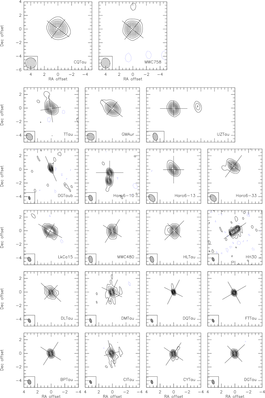
Figure 1: High angular resolution image of the continuum emission from the sources observed in the survey at 1.3 mm (230 GHz). The contours are relative to the peak intensity, in steps of 10 %. Coordinates are offsets in arcseconds from the reference positions given in Table 2

Figure 1 is a montage of the 1.3 mm images of the survey sources, presented in terms of fraction of the peak flux. Figure 2 is as Fig.1, but for 2.7 or 3.4 mm, depending on the sources. Robust weighting was used to produce these images. Despite the fairly wide range of angular resolutions (from $0.5\times 0.3^{\prime\prime}$ to about $1.5^{\prime\prime}$), clearly some objects are much more centrally condensed than others. In particular, the most compact sources are the two circumstellar disks in the Haro 6-10 binary.

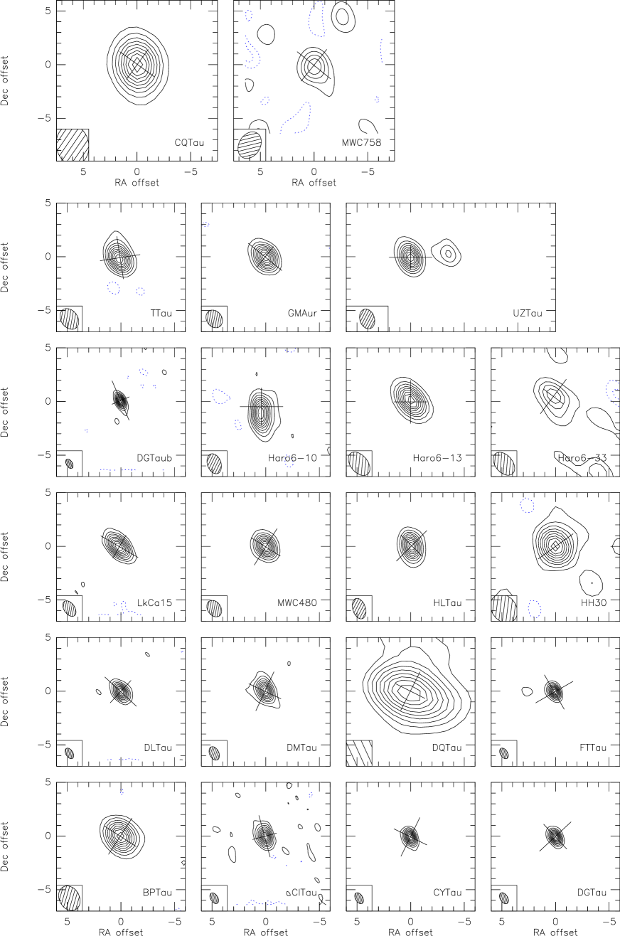
Figure 2: High angular resolution image of the continuum emission from the sources observed in the survey at 2.7 or 3.4 mm. The contours are relative to the peak intensity, in steps of 10%, except for the weakest sources (Haro 6-33 & MWC 758) for which the step is 20 %.

3 Modeling

3.1 Simple analysis

The measured flux densities at 1.3 mm and around 3 mm are given in Table 3 (considering only baselines shorter than 100 m). They result from a simple elliptical Gaussian fit to the $uv$ data. For the orientations and apparent sizes, all baselines were included. Short baseline data, although adequate to measure the overall flux densities and apparent spectral index $\alpha$, are not suitable to derive characteristic sizes and even position angles. This is because, to first order, disks have power law distributions of the surface density and temperature and are optically thin at such wavelengths. Thus, when seen at low inclination, ($<45^{\circ}$ or so), the surface brightness is a power law of the radius and has no characteristic size. This can bias the apparent position angle, since the apparent half-power size only depends on the angular resolution and the exponent of the power law. For nearly edge-on disks ($i>75^{\circ}$), the disk thickness introduces a characteristic size, because the brightness falls off like a Gaussian in this direction, so the position angle is properly recovered. Thus, in general, reliable position angles can only be derived with sufficient angular resolution, i.e. from long baseline fits. These properties can explain the different position angles found by previous authors using lower resolution data (e.g. Dutrey et al. 1996; Kitamura et al. 2002). Note that these biases on the position angles can also affect analysis made with more elaborate disk models: only sufficiently high angular resolution can provide an unbiased determination of this parameter.

On the other hand, for sources with an apparent core-halo structure, such as DM Tau or CI Tau, the long baseline fit tends to represent only the central part and misses substantial flux. The spectral index $\alpha_{100}$ derived from long baseline data (Table 3, Col.8) is systematically smaller than that from the short baseline fit only (Col.7). This indicates either a contribution of an optically thick core and/or dust grain evolution.

Figure 3: Top: disk inclinations measured from dust and other methods (CO or jets). Bottom: Position angle of the disk rotation axis derived from dust and other methods. The only discrepant points are for BP Tau (orientation) and DG Tau-b (inclination).

3.2 Model description

Because the apparent size, orientation, and spectral index may depend on the $uv$ coverage when using a simple Gaussian model, we must analyze the data with more realistic brightness distributions. Because a direct inversion of the brightness profile is impossible, due to the combination of insufficient resolution and the limited signal-to-noise, a global fitting technique using some a-priori model must be used. We therefore analyzed the continuum emission in terms of two “standard” disk models that differ only in the surface density distribution. Model 1 uses a simple truncated power law, Model 2 an exponentially tapered power law with an arbitrarily large outer radius. The surface density is characterized by three parameters plus an inner radius in each model. Our approach is to keep the model parametric and simple to avoid as much as possible biases towards a specific physical model for disks.

In Model 1, the surface density is a simple power law with a sharp inner and outer radius:

$$\Sigma(r)=\Sigma_{0}\left(\frac{r}{r_{0}}\right)^{-p},$$ (4)

for $R_{\mathrm{int}}<r<R_{\mathrm{out}}$.

In Model 2, the density is tapered by an exponential edge:

$$\Sigma(r)=\Sigma_{0}\left(\frac{r}{R_{0}}\right)^{-\gamma}\exp\left(-(r/R_{c})^{2-\gamma}\right).$$ (5)

Note that Model 1 derives from Model 2 by simply setting $R_{c}\rightarrow\infty$ and $p=\gamma$ in the above parametrization. Model 2 is a solution of the self-similar evolution of a viscous disk in which the viscosity is a power law of the radius (with constant exponent in time $\gamma$).

With the inner ($R_{\mathrm{int}}$) and outer ($R_{\mathrm{out}}$) radii, the disk mass is given by

$$M_{d}=\frac{2\pi R_{0}^{2}\Sigma_{0}}{2-\gamma}\left(\frac{R_{c}}{R_{0}}\right)^{2-\gamma}\left(\exp\left(-\left(\frac{R_{\mathrm{int}}}{R_{c}}\right)^{2-\gamma}\right)-\exp\left(-\left(\frac{R_{\mathrm{out}}}{R_{c}}\right)^{2-\gamma}\right)\right),$$ (6)

which for small $R_{\mathrm{int}}$ and large $R_{\mathrm{out}}$ yields

$$M_{d}=\frac{2\pi R_{0}^{2}\Sigma_{0}}{2-\gamma}\left(\frac{R_{c}}{R_{0}}\right)^{2-\gamma}.$$ (7)

The simple power law case is recovered for $R_{c}\rightarrow\infty$, by developing to first order in $(r/R_{c})^{2-\gamma}$,

$$M_{d}=\frac{2\pi R_{0}^{2}\Sigma_{0}}{2-\gamma}\left(\left(\frac{R_{\mathrm{out}}}{R_{0}}\right)^{2-\gamma}-\left(\frac{R_{\mathrm{int}}}{R_{0}}\right)^{2-\gamma}\right).$$ (8)

One can also used $M_{d}$ as a free parameter instead of $\Sigma_{0}$, like in Andrews et al. (2009). Eq.6 can also be used to show that $R_{c}$ is the radius which contains 63 % of the disk mass, because $M(r<R_{c})=M_{d}(1-1/e)=0.63M_{d}$ provided $R_{\mathrm{out}}$ is large enough.

An equivalent parametrization is that described by Isella et al. (2009)

$$\Sigma(r)=\Sigma_{t}\left(\frac{R_{t}}{r}\right)^{\gamma}\exp\left(\frac{1-(r/R_{t})^{2-\gamma})}{2(2-\gamma)}\right).$$ (9)

The parameterizations using $R_{t}$ or $M_{d}$ become ill defined for $\gamma=2$, which makes them less suited for use in a minimization scheme than the simple parametric expression of Eq.5 (for which only $R_{c}$ is unconstrained, as the surface density becomes a power law). $R_{t}$ is related to $R_{c}$ by

$$R_{t}=R_{c}\left(\frac{1}{2(2-\gamma)}\right)^{\frac{1}{2-\gamma}}.$$ (10)

$R_{t}/R_{c}$ is close to 0.5 for all values of $\gamma$ below 1, reaches 1 for $\gamma=1.5$, then diverges for $\gamma\rightarrow 2$. In the framework of self-similar viscous evolution (Lynden-Bell & Pringle 1974; Hartmann et al. 1998), it can be shown that $R_{t}$ is the radius at which the net mass flux changes sign.

In both models, the temperature is assumed to be a simple power law of the radius

$$T(r)=T_{0}(r/R_{0})^{-q}.$$ (11)

The disks are thus vertically isothermal. To allow a homogeneous comparison, we used $T_{100}=T(100\leavevmode\nobreak\ \mathrm{AU})=15$ K and $q=0.4$, except when those parameters can be constrained by the observations. The validity and impact of this assumption will be discussed in Sec.4.1.

Similar analyses have been used by Kitamura et al. (2002) and Andrews & Williams (2007) for their 2 mm and 0.8 mm data respectively. Most previous studies (Kitamura et al. 2002; Andrews & Williams 2007; Isella et al. 2009) used the thin disk approximation to compute visibilities. Here, because our sample includes highly inclined objects, we assume that the disks are flared, with a scale height varying as a power law of the radius $h(r)=H_{100}(r/100\mathrm{AU})^{-h}$. For all but the two highly inclined objects (HH 30 and DG Tau-b), we used $H_{100}=16$ AU and $h=-1.25$. These values agree with those derived using the gas temperature determined from CO observations whenever available, and the stellar mass, either from kinematic determination (Simon et al. 2000) or standard evolutionary tracks. The results are, however, completely independent of the assumed scale height, which justifies a posteriori the thin disk approximation used by previous authors. However, for the two highly inclined objects, $H_{100}$ and the exponent $h$ had to be used as adjustable parameters.

The inner radius $R_{\mathrm{int}}$ is also not significant in general, except for a few special sources that display inner cavities, such as GM Aur, HH 30 and LkCa 15 (see Sec.4.4.2). We fixed it to 1 AU, but in general, any value lower than about 3-4 AU would not change the results. For Model 2, we used for $R_{\mathrm{out}}$ the outer radius derived from CO observations when available. If not, we set it to 500 AU. These outer radii are large enough to have negligible influence on the results.

Each model has thus a priori five free intrinsic parameters: two for temperature $T_{0}$ and $q$, three for the surface density $\Sigma_{0}$, $p$ or $\gamma$, and $R_{\mathrm{out}}$ or $R_{c}$, plus the inclination, orientation and position.

The dust opacity as a function of wavelength and radius completes the description. In a first step, we assume it to be independent of radius and described by the following prescription

$$\kappa(\nu)=\kappa_{230}(\nu/230\mathrm{GHz})^{\beta_{m}},$$ (12)

with $\kappa_{230}=2\leavevmode\nobreak\ \mathrm{cm}^{2}{\rm g}^{-1}$ (per gram of dust). This introduces one additional parameter, the mean dust emissivity index $\beta_{m}$. This is similar to the Beckwith et al. (1990) results, but using a different pivot frequency to avoid further dependence of the derived disk mass on $\beta$. The dust model used by Andrews & Williams (2007) and Andrews et al. (2009) also results in $\beta_{m}=1$, but with a slightly different absorption coefficient $\kappa_{230}=2.2\leavevmode\nobreak\ \mathrm{cm}^{2}{\rm g}^{-1}$. Finally, we also assume that the gas-to-dust ratio is constant and equal to 100. In a second step, we shall relax the assumption of constant $\kappa(\nu)$ as a function of radius $r$, see Sec.4.5.

Appendix A (available on-line only) illustrates some of the possible degeneracy between the various models, in particular between constant dust properties with an optically thick inner region, and variable dust properties.

3.3 Fitting method

For the inclination and orientation, we used the accurate determination from the CO kinematics when possible. Values derived from optical observations (scattered light images, or optical jets) or molecular jets were used for some sources for which the disk kinematics is not known. Independent fits of these parameters from the dust emission were also performed to check the consistency of the results: see Table 4 and references therein. We stress, however, that the uncertainties on the disk inclination and orientation do not significantly affect the derived radial structure.

At each observed frequency, the radiative transfer equation is solved by a simple ray-tracing algorithm, and model images are generated. Great care has been taken to avoid numerical precision problems caused by finite grid effects. The numerical integration is typically performed on a 128 x 128 grid, with 512 points along the line of sight. Two oversampling techniques are used to enhance the accuracy while keeping computational costs reasonable. First, the overall image is interpolated (by bilinear interpolation) by a factor 2 before computing the model visibilities. Second, the inner 64 x 64 pixels are re-computed on this finer grid with a smaller step along the line of sight (64 x 64 x 1024). Larger numbers were used for the largest disk. This results in effective pixel sizes of 2 to 7 AU in (x,y), depending on the outer disk radius used in the model, and steps 4 to 8 times smaller along the line of sight.

A modified Levenberg-Marquardt method was used to derive the disk parameters by a non-linear least squares fit of the modeled visibilities directly to the observed $uv$ data, as detailed by Piétu et al. (2007). Like all methods, L-M minimization can be trapped in local minima when the starting point is too far away from the solution. We alleviate this problem by using multiple re-starts when needed, and also by adapting the step size used to compute the gradient. We found empirically that using steps equal to half a sigma on each parameter provided stable results. Error bars were derived from the covariance matrix, except when the parameter coupling was too strong (e.g. between $R_{c}$ and $\gamma$ in Model 2 for $\gamma$ larger than about 1.5). In that case, the multi-parameter fit was reduced to a one parameter problem by finding the best fit for several values of this parameter, and determining the error bars from the resulting $\chi^{2}$ distribution. Data at several available wavelengths are fitted simultaneously by the same model, which allows us to constrain $\beta_{m}$. However, whenever data at very nearby frequencies (220 and 230 GHz, for example) exist, only one was considered in this process, because even small absolute calibration error could result in a strong bias on the value of $\beta_{m}$. In the dual frequency fit, the long wavelength (2.7 or 3.4 mm) data do not in general influence the derived surface density law, because of their lower angular resolution, but only serve to determine $\beta_{m}$. Because the geometric parameters are largely decoupled from the disk intrinsic parameters, the simultaneous fit of dual-frequency data sets used (in general) four parameters: $\Sigma_{0}$, $p$ ($\gamma$ in Model 2), $R_{\mathrm{out}}$ (or $\gamma$ and $R_{c}$ in Model 2), and $\beta_{m}$. Additional parameters ($T_{0},q$ or $H_{0},h$) were also fitted simultaneously when needed. Separate fits were also made at 1.3 and 2.7 mm for the few sources were the angular resolution at 2.7 mm is sufficient, or when data sets at 1.4 mm also existed: in these cases, $\beta_{m}$ was set at the value found from the dual frequency analysis, and only the three remaining parameters were fitted together.

The choice of the pivot radius $R_{0}$ in Equations 4-5 is important. There is always an optimal value that minimizes the error on $\Sigma_{0}$, which depends on the angular resolution and source surface density profile (see discussion in Piétu et al. 2007). Using a non-optimal value results in a coupling of $\Sigma_{0}$ with $p$ for Model 1, and $\gamma,R_{c}$ in Model 2. Another different pivot radius is also required for $T_{0}$ when the source is sufficiently optically thick and resolved to constrain $T_{0},q$.

Two stars required a specific treatment: the binary Haro 6-10 and the quadruple UZ Tau, which have two disks in the field of view. For Haro 6-10, a simple Gaussian model of the emission from the other disk was subtracted before the analysis of each disk. For UZ Tau, the procedure was more elaborate. First a Gaussian model of the emission from the companion (UZ Tau W) was subtracted, and the remaining emission from UZ Tau E was analyzed. Then, the best-fit model of UZ Tau E was subtracted from the original data, and the emission from UZ Tau W analyzed separately.

Figure 4: Transition radius (bottom) and characteristic exponent $\gamma$ derived from independent data sets.

Table 4: Derived inclinations

Source	$PA$	$i$	$PA_{\mathrm{CO}}$	$i_{\mathrm{CO}}$
	∘	∘	∘	∘
BP Tau	107$\pm$ 5	39$\pm$ 3	-119$\pm$ 2	33$\pm$ 6
CI Tau	285$\pm$ 5	55$\pm$ 5	285$\pm$ 1	44$\pm$ 3
CQ Tau	-37$\pm$ 19	-31$\pm$ 10	-36$\pm$ 1	-29$\pm$ 2
CY Tau	63$\pm$ 5	34$\pm$ 3	63$\pm$ 1	28$\pm$ 5
DG Tau	60$\pm$ 4	32$\pm$ 2	43$\pm$ 2	38$\pm$ 2
DG Tau b	114$\pm$ 1	64$\pm$ 2	117$\pm$ 3	$>75$
DL Tau	141$\pm$ 3	38$\pm$ 2	144$\pm$ 3	43$\pm$ 3
DM Tau	67$\pm$ 5	-36$\pm$ 3	63$\pm$ 1	-34$\pm$ 1
FT Tau	31$\pm$ 14	21$\pm$ 5	29$\pm$ 4	23$\pm$ 14
GM Aur	139$\pm$ 3	54$\pm$ 3	144$\pm$ 1	50$\pm$ 1
HL Tau	42$\pm$ 2	45$\pm$ 1	45	45
LkCa 15	150$\pm$ 2	48$\pm$ 2	150$\pm$ 1	52$\pm$ 1
MWC 480	75$\pm$ 5	30$\pm$ 2	58$\pm$ 1	37$\pm$ 1
MWC 758	147$\pm$ 292	-11$\pm$ 249	141$\pm$ 1	18$\pm$ 36
UZ Tau E	-3$\pm$ 3	131$\pm$ 2	-4$\pm$ 2	124$\pm$ 2
UZ Tau W	-34$\pm$ 14	124$\pm$ 12	-4$\pm$ 2	124$\pm$ 2
HH 30	35$\pm$ 1	98$\pm$ 1	32$\pm$ 3	99$\pm$ 3

Position angles are those of the disk rotation axis. The inclinations $i_{\mathrm{CO}}$ have been derived from CO observations except for UZ Tau W (assumed to be equal to that of UZ Tau E), DG Tau, and DG Tau-b, which come from Eislöffel & Mundt (1998). For HL Tau, the CO outflow defines $i_{\mathrm{CO}}$ and $PA_{\mathrm{CO}}$. Conventions for PA and $i$ use the rotation axis orientation as described by Piétu et al. (2007).

Table 5: Derived parameters for the viscous and power law models

(1)	(2)	(3)	(4)	(5)	(6)	(7)	(8)	(9)	(10)
Source	Mass	$R_{c}$	$R_{t}$	$\gamma$	$\Delta\chi^{2}$	$\Sigma_{100}$	$R_{\mathrm{out}}$	p	$\beta_{m}$
	$0.001\,\mathrm{M_{\odot}}$	AU	AU			g.cm-2	AU
BP Tau	5.4$\pm$ 0.2	43$\pm$ 2	22$\pm$ 1	-0.04$\pm$ 0.12	14	3.88$\pm$ 0.11	57$\pm$ 1	0.40$\pm$ 0.07	0.65$\pm$ 0.04
CI Tau	37.1$\pm$ 2.7	166$\pm$ 10	81$\pm$ 4	0.30$\pm$ 0.04	33	2.59$\pm$ 0.06	201$\pm$ 4	0.59$\pm$ 0.03	0.68$\pm$ 0.05
CQ Tau	6.3$\pm$ 0.4	86$\pm$ 8	41$\pm$ 3	0.61$\pm$ 0.25	0	0.49$\pm$ 0.03	188$\pm$ 30	1.35$\pm$ 0.15	0.75$\pm$ 0.05
CY Tau	16.5$\pm$ 0.6	67$\pm$ 2	32$\pm$ 1	0.28$\pm$ 0.06	35	3.55$\pm$ 0.07	92$\pm$ 2	0.82$\pm$ 0.04	0.16$\pm$ 0.03
DG Tau	36.0$\pm$ 2.0	9$\pm$ 2	12$\pm$ 8	1.56$\pm$ 0.11	-33	3.51$\pm$ 0.06	198$\pm$ 27	2.74$\pm$ 0.08	1.31$\pm$ 0.05
DL Tau	49.0$\pm$ 1.0	148$\pm$ 4	72$\pm$ 2	0.37$\pm$ 0.03	63	4.48$\pm$ 0.04	179$\pm$ 2	0.67$\pm$ 0.02	0.70$\pm$ 0.03
DM Tau	31.1$\pm$ 1.6	180$\pm$ 10	86$\pm$ 5	0.54$\pm$ 0.03	-17	2.65$\pm$ 0.03	274$\pm$ 16	0.56$\pm$ 0.02	0.78$\pm$ 0.04
DQ Tau (*)	12.1$\pm$ 4.2	11$\pm$ 20	25$\pm$ 50	1.63$\pm$ 0.13	-278	0.43$\pm$ 0.01	439$\pm$ 534	2.03$\pm$ 0.06	0.35$\pm$ 0.15
FT Tau	7.7$\pm$ 0.3	43$\pm$ 1	21$\pm$ 1	-0.17$\pm$ 0.09	13	5.31$\pm$ 0.12	57$\pm$ 0	0.40$\pm$ 0.06	-0.13$\pm$ 0.04
GM Aur (*)	27.0$\pm$ 3.6	98$\pm$ 24	$>80$	1.53$\pm$ 0.07	3	2.55$\pm$ 0.02	578$\pm$ 184	2.02$\pm$ 0.05	1.02$\pm$ 0.06
LkCa 15	28.4$\pm$ 1.4	109$\pm$ 3	55$\pm$ 1	-0.23$\pm$ 0.17	17	4.90$\pm$ 0.10	178$\pm$ 7	1.66$\pm$ 0.12	1.27$\pm$ 0.05
MWC 480	182.3$\pm$ 11.2	81$\pm$ 5	39$\pm$ 4	0.75$\pm$ 0.17	28	9.08$\pm$ 0.15	155$\pm$ 6	1.86$\pm$ 0.07	1.74$\pm$ 0.05
MWC 758	10.6$\pm$ 1.5	102$\pm$ 27	52$\pm$ 15	0.54$\pm$ 0.52	0	0.95$\pm$ 0.07	187$\pm$ 50	1.09$\pm$ 0.30	1.53$\pm$ 0.27
UZ Tau E	24.1$\pm$ 0.7	79$\pm$ 2	39$\pm$ 1	0.12$\pm$ 0.08	27	4.96$\pm$ 0.15	115$\pm$ 5	0.72$\pm$ 0.07	0.74$\pm$ 0.04
UZ Tau W	3.5$\pm$ 0.2	50$\pm$ 2	23$\pm$ 8	1.05$\pm$ 0.46	-1	0.35$\pm$ 0.02	128$\pm$ 43	1.66$\pm$ 0.21	0.39$\pm$ 0.14
HL Tau	90.6$\pm$ 4.1	40$\pm$ 15	22$\pm$ 2	1.32$\pm$ 0.08	-75	12.73$\pm$ 0.35	280$\pm$ 26	2.62$\pm$ 0.11	1.97$\pm$ 0.07
HH 30	8.1$\pm$ 0.4	102$\pm$ 2	62$\pm$ 2	-2.41$\pm$ 0.42	0	2.50$\pm$ 0.11	123$\pm$ 3	-0.56$\pm$ 0.39	0.47$\pm$ 0.08
DG Tau b (*)	67.9$\pm$ 29.6	81$\pm$ 15	48$\pm$ 18	1.18$\pm$ 0.18	-7	5.67$\pm$ 1.49	303$\pm$ 23	1.95$\pm$ 0.10	0.94$\pm$ 0.12
T Tau	0.1$\pm$ 0.05	8$\pm$ 2	8$\pm$ 2	-1$\pm$ 1	-6	$>5$	67$\pm$ 20	[1]	0.48$\pm$ 0.50
Haro 6-10 N	0.6$\pm$ 0.1	17$\pm$ 3	5$\pm$ 3	[0]	3	$>10$	14$\pm$ 1	[1]	[1.0]
Haro 6-10 S	0.5$\pm$ 0.1	10$\pm$ 2	4$\pm$ 3	[0]	0	$>10$	14$\pm$ 1	[1]	[1.0]
Haro 6-13	17.3$\pm$ 7.7	19$\pm$ 41	10$\pm$ 1	1.00$\pm$ 2.39	2	3.56$\pm$ 1.26	90$\pm$ 32	1.03$\pm$ 0.94	0.08$\pm$ 0.07
Haro 6-33	6.8$\pm$ 1.6	$>50$	-	1.48$\pm$ 0.15	0	0.28$\pm$ 0.02	439$\pm$ 616	1.57$\pm$ 0.17	0.41$\pm$ 0.26

(*) Error bars on $R_{t}$ to be considered with caution, see text. Negative $\Delta\chi^{2}$ indicates that the power law model is better. Values in brackets indicate fixed parameters.

Table 6: Comparison of values derived from independent data sets at similar wavelengths

Source	$R_{out}$	$p$	$R_{out}$	$p$	$R_{t}$	$\gamma$	$R_{t}$	$\gamma$
	AU		AU		AU		AU
	at 1.3 mm		at 1.4 mm		at 1.3 mm		at 1.4 mm
LkCa 15	198$\pm$ 15	1.59$\pm$ 0.19	179$\pm$ 8	1.62$\pm$ 0.11	60$\pm$ 2	0.08$\pm$ 0.23	56$\pm$ 1	-0.20$\pm$ 0.16
MWC480	153$\pm$ 6	1.77$\pm$ 0.09	188$\pm$ 8	1.75$\pm$ 0.06	41$\pm$ 3	0.52$\pm$ 0.22	59$\pm$ 8	0.72$\pm$ 0.12

Table 7: Comparison of values derived from two different wavelengths

Source	$R_{out}$	$p$	$R_{out}$	$p$	$R_{t}$	$\gamma$	$R_{t}$	$\gamma$
	AU		AU		AU		AU
	at 1.3 mm		at 2.8 mm		at 1.3 mm		at 2.8 mm
CI Tau	215$\pm$ 6	0.58$\pm$ 0.03	186$\pm$ 13	0.61$\pm$ 0.10	98$\pm$ 8	0.36$\pm$ 0.04	63$\pm$ 5	0.03$\pm$ 0.17
CY Tau	104$\pm$ 3	0.90$\pm$ 0.03	108$\pm$ 10	1.22$\pm$ 0.12	35$\pm$ 2	0.35$\pm$ 0.06	29$\pm$ 2	0.47$\pm$ 0.20
DG Tau	188$\pm$ 30	2.69$\pm$ 0.10	401$\pm$ 7	2.89$\pm$ 0.02	12$\pm$ 2	1.55$\pm$ 0.17	11$\pm$ 1	1.58$\pm$ 0.33
DL Tau	181$\pm$ 1	0.65$\pm$ 0.02	146$\pm$ 7	0.72$\pm$ 0.09	75$\pm$ 2	0.38$\pm$ 0.03	50$\pm$ 3	0.19$\pm$ 0.14
DM Tau	285$\pm$ 24	0.55$\pm$ 0.02	250$\pm$ 37	0.76$\pm$ 0.07	94$\pm$ 6	0.56$\pm$ 0.03	67$\pm$ 9	0.60$\pm$ 0.13
FT Tau	57$\pm$ 1	0.41$\pm$ 0.06	85$\pm$ 12	1.03$\pm$ 0.24	21$\pm$ 1	-0.20$\pm$ 0.10	23$\pm$ 2	0.05$\pm$ 0.42
LkCa 15	198$\pm$ 15	1.59$\pm$ 0.19	168$\pm$ 33	1.70$\pm$ 0.65	60$\pm$ 2	0.08$\pm$ 0.23	53$\pm$ 6	-0.23$\pm$ 0.84
MWC 480	153$\pm$ 6	1.77$\pm$ 0.09	170$\pm$ 51	2.07$\pm$ 0.32	41$\pm$ 3	0.52$\pm$ 0.22	45$\pm$ 22	1.08$\pm$ 0.52

All results are presented in Table 5. A comparison of the results obtained from independent data sets at similar wavelengths is shown in Table 6, which shows the excellent agreement of the constrained parameters (see also Fig.4). In addition, the good agreement of geometric parameters with determinations from other studies is a further proof of the data quality (see Table 4, and Fig.3).

Simple power law

Results for the surface density parameters, $\Sigma_{100},p$ and $R_{\mathrm{out}}$, are presented in Col. 7-10 of Table 5. For most sources, the emission is largely optically thin, so the derived surface density will scales as roughly $1/T_{0}$, but the outer radius remains essentially unaffected by the choice of the temperature. The only exceptions are the T Tau and Haro 6-10, which are essentially optically thick disks. FT Tau and Haro 6-13 may also be attributed to thick disks.

Exponential edge

We generally used Eq.5 to first locate the minimum. However, because of the direct dependency between the parameters, the errors on $R_{t}$ and $M_{d}$ were obtained by re-fitting the data using these parameters as primary parameters rather than $R_{c}$ and $\Sigma_{0}$. Note that while the error on $\Sigma_{t}$ may become very large, $\Sigma_{0}$ is generally constrained with a very similar accuracy as in Model 1.

Results are presented in Cols 2-5 of Table 5. It was difficult to adjust this model to a few sources, among which were the apparently optically thick sources T Tau and Haro 6-10, and the single stars DQ Tau, DG Tau-b, and GM Aur. For the three latter stars, the best-fit power law has an index of $p=2$. In this case, the expression in Eq.5 attempts to fit $\gamma=2$ and diverges. Finding the best fit requires the determination of the best transition radius $R_{c}$ and its errorbar for all values of $\gamma$ ranging from 0.6 to 1.9 (by steps of 0.1). The relative errors on $R_{t}$ are generally larger than for $R_{c}$, because $R_{t}/R_{c}$ diverges for $\gamma\rightarrow 2$. No constraint on $R_{t}$ is possible for DQ Tau. For GM Aur, only a lower limit is obtained, while for DG Tau-b, $R_{t}$ is very marginally constrained: at the $2\sigma$ level, any value is acceptable. The error bars should be taken with care in those cases. A similar procedure was used for Haro 6-13 and Haro 6-33, for which $R_{t}$ remains unconstrained at the $2\sigma$ level.

Col 6 of Table 5 indicates the difference in $\chi^{2}$ between Model 1 and Model 2. A positive value indicates Model 2 (the viscous disk) provides an apparently better fit than the truncated power law. The significance of this result will be discussed in Section 5.2.

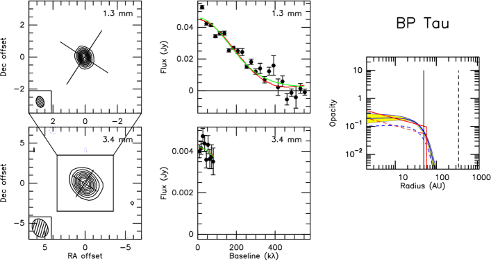
Figure 21: As Fig.5 but for BP Tau. Contour level is 3 mJy/beam ($6\sigma$) at 1.3 mm, and 0.4 mJy/beam ($3\sigma$) at 3.4 mm.

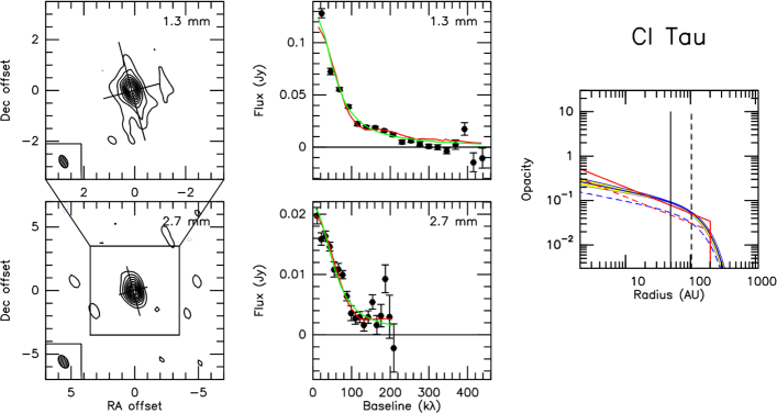
Figure 22: As Fig.5 but for CI Tau. Contour level is 2.2 mJy/beam ($3.5\sigma$) at 1.3 mm, and 0.86 mJy/beam ($2\sigma$) at 2.7 mm.

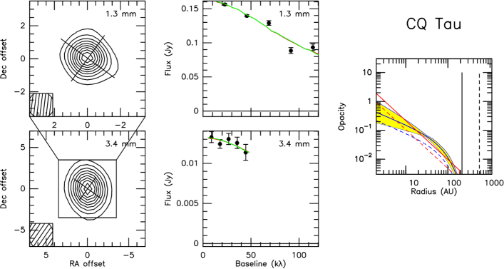
Figure 23: As Fig.5 but for CQ Tau.

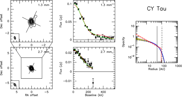
Figure 24: As Fig.5 but for CY Tau. Contour level is 3.3 mJy/beam ($4\sigma$) at 1.3 mm, and 1.6 mJy/beam ($4\sigma$) at 2.7 mm.

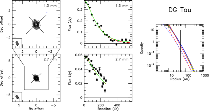
Figure 25: As Fig.5 but for DG Tau. Contour level is 16 mJy/beam ($5\sigma$) at 1.3 mm, and 4.3 mJy/beam ($4.3\sigma$) at 2.7 mm.

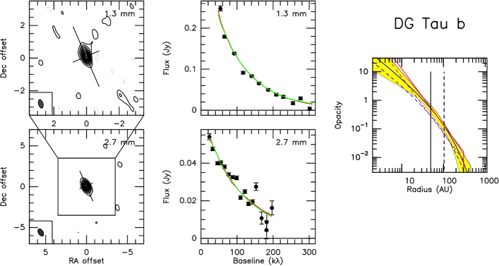
Figure 26: As Fig.5 but for DG Tau b. Contour level is 7.4 mJy/beam ($3.7\sigma$) at 1.3 mm, and 3.2 mJy/beam ($3.2\sigma$) at 2.7 mm.

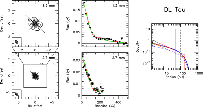
Figure 27: As Fig.5 but for DL Tau. Contour level is 4.3 mJy/beam ($5.5\sigma$) at 1.3 mm, and 1.4 mJy/beam ($3.5\sigma$) at 2.7 mm.

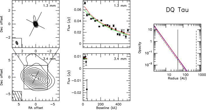
Figure 28: As Fig.5 but for DQ Tau. Contour level is 3.6 mJy/beam ($4.5\sigma$) at 1.3 mm, and 0.8 mJy/beam ($1.6\sigma$) at 3.4 mm.

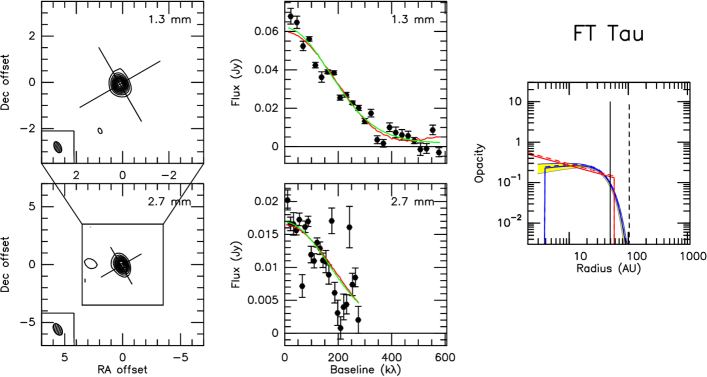
Figure 29: As Fig.5 but for FT Tau. Contour level is 2.6 mJy/beam ($8\sigma$) at 1.3 mm, and 1.3 mJy/beam ($6\sigma$) at 2.7 mm.

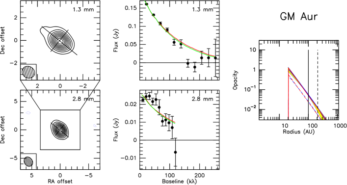
Figure 30: As Fig.5 but for GM Aur. Contour level is 10 mJy/beam ($65\sigma$) at 1.3 mm, and 1.9 mJy/beam ($3.2\sigma$) at 2.8 mm.

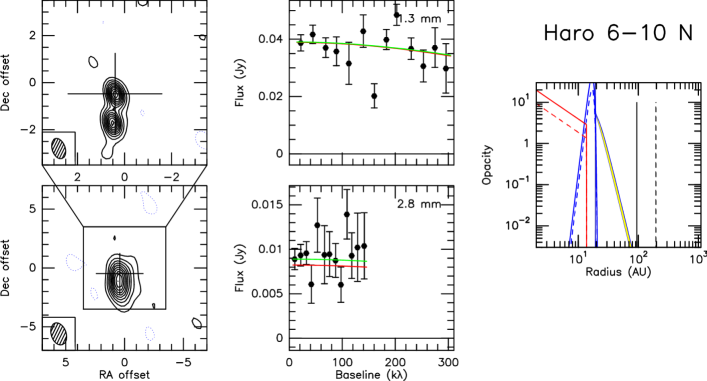
Figure 31: As Fig.5 but for Haro 6-10 N. Contour level is 3.5 mJy/beam ($4\sigma$) at 1.3 mm, and 1.2 mJy/beam ($3\sigma$) at 2.8 mm.

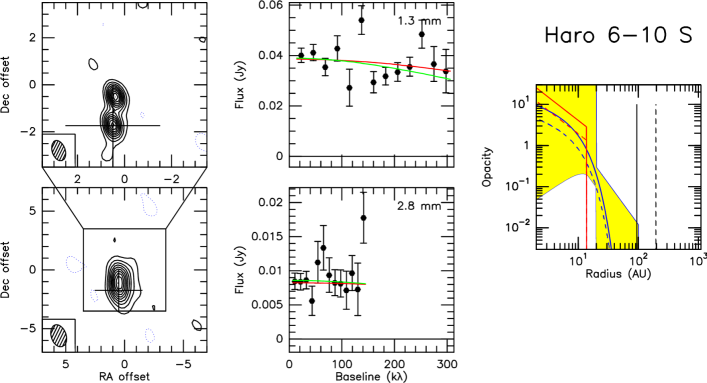
Figure 32: As Fig.5 but for Haro 6-10 S. Contour level is 3.5 mJy/beam ($4\sigma$) at 1.3 mm, and 1.2 mJy/beam ($3\sigma$) at 2.8 mm.

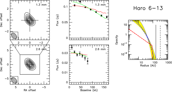
Figure 33: As Fig.5 but for Haro 6-13. Contour level is 8.3 mJy/beam ($5\sigma$) at 1.3 mm, and 2.8 mJy/beam ($5.6\sigma$) at 2.6 mm.

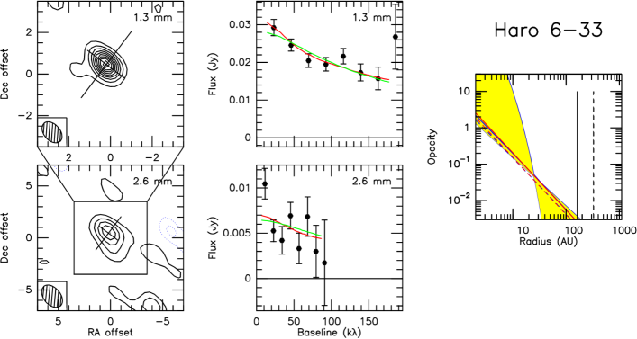
Figure 34: As Fig.5 but for Haro 6-33. Contour level is 2 mJy/beam ($3.3\sigma$) at 1.3 mm, and 1.5 mJy/beam ($1.7\sigma$) at 2.6 mm.

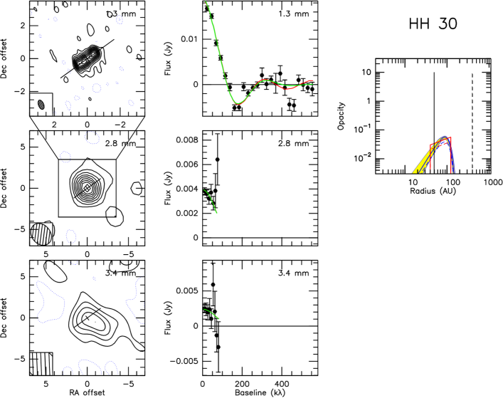
Figure 35: As Fig.5 but for HH 30. Contour level is 0.4 mJy/beam ($2\sigma$) at 1.3 mm, 0.5 mJy/beam ($1.2\sigma$) at 3.4 mm, and 0.36 mJy/beam ($2.2\sigma$) at 2.8 mm.

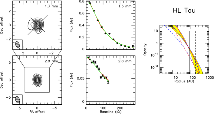
Figure 36: As Fig.5 but for HL Tau. Contour level is 32 mJy/beam ($4.5\sigma$) at 1.3 mm, and 7.3 mJy/beam ($9\sigma$) at 2.8 mm.

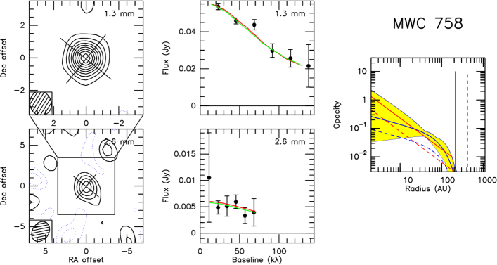
Figure 37: As Fig.5 but for MWC 758. Contour level is 4 mJy/beam ($2.7\sigma$) at 1.3 mm, and 0.8 mJy/beam ($1.3\sigma$) at 2.6 mm.

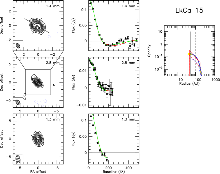
Figure 38: As Fig.5 but for Lk Ca 15. Contour level is 2.6 mJy/beam ($4\sigma$) at 1.4 mm, 1.0 mJy/beam ($3\sigma$) at 2.8 mm, and 7.9 mJy/beam ($5\sigma$) at 1.3 mm.

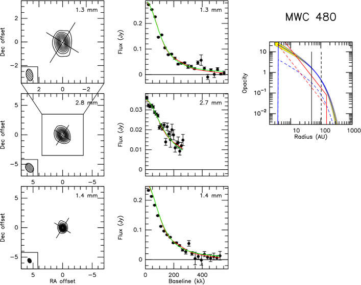
Figure 39: As Fig.5 but for MWC 480. Contour level is 15 mJy/beam ($5.8\sigma$) at 1.3 mm, 2.9 mJy/beam ($7\sigma$) at 2.8 mm, and 12 mJy/beam ($5.5\sigma$) at 1.4 mm.

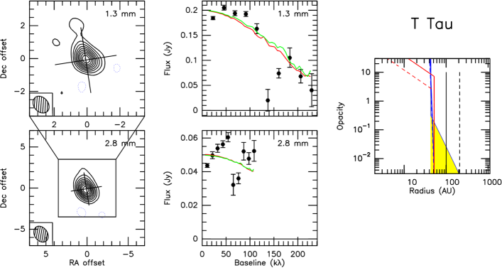
Figure 40: As Fig.5 but for T Tau. Contour level is 16 mJy/beam ($3\sigma$) at 1.4 mm, and 4.8 mJy/beam ($4.8\sigma$) at 2.8 mm.

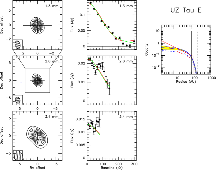
Figure 41: As Fig.5 but for UZ Tau E. Contour level is 8.6 mJy/beam ($6\sigma$) at 1.3 mm, 1.9 mJy/beam ($4.7\sigma$) at 2.8 mm, and 1.3 mJy/beam ($4\sigma$) at 3.4 mm.

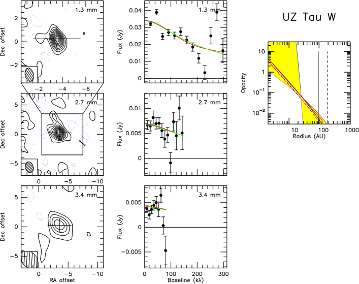
Figure 42: As Fig.5 but for UZ Tau W. Contour level is 2.6 mJy/beam ($1.9\sigma$) at 1.3 mm, 0.6 mJy/beam ($1.5\sigma$) at 2.8 mm, and 0.7 mJy/beam ($2\sigma$) at 3.4 mm.

Deprojected, circularly averaged visibility profiles are displayed in the middle column of Figure 5 for DM Tau and Figures 21-42 for the others sources (in Appendix G, available on-line only). These deprojected visibilities only serve as an illustration of the fit results, but not to determine the parameter values and their errors.

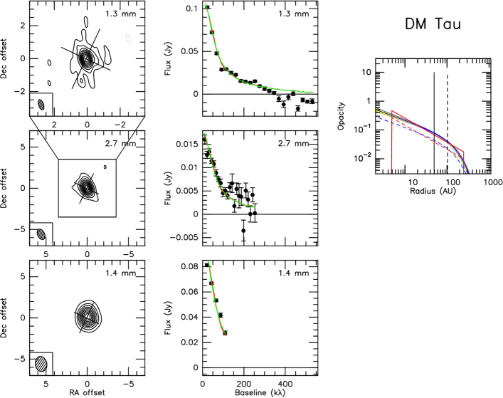
Figure 5: Left row: High angular resolution images of DM Tau. On top, high resolution 1.3 mm image, in the middle, the 2.7 mm (or 3.4 mm for some sources) image with a box indicating the size of the 1.3 mm view. For sources (like this one) that have independent data sets at other wavelengths (1.4 or 3.4 mm), a lower panel displays the corresponding image for the same area as above. All contours are 10 % of the peak value to illustrate consistently the apparent sizes and low level extensions. Contour level is 2 mJy/beam ($3.5\sigma$) at 1.3 mm, 0.78 mJy/beam ($2\sigma$) at 2.7 mm, and 6 mJy/beam ($7\sigma$) at 1.4 mm. Middle row: Deprojected and circularly averaged visibilities and best-fit models for each wavelength. Red is for power law, green for exponential edge. Right panel: Best-fit opacity profile (perpendicular to the disk plane, i.e. $\kappa_{\nu}\Sigma(r)$) for the 1.3 mm and long wavelength models. The continuous line is for the short wavelength, the dashed line for the long wavelength. The vertical lines indicate the effective angular resolution.

4 Results

4.1 The dust temperature

For the assumed temperature law, our treatment differs quite significantly from those of Kitamura et al. (2002) and Andrews & Williams (2007), who assumed that the temperature derived from IR-emitting dust by fitting the SED also applies to the mm emitting dust. However, strong vertical temperature gradients are expected in disks (e.g. D’Alessio et al. 1999).

Because the mm emission comes from cold dust around the disk mid-plane, using a power law for the dust temperature distribution is an oversimplification. The dust temperature is expected to follow three different regimes, depending on whether the disk is optically thick or thin for absorption of the incident radiation and re-emission of its own radiation. The two extreme regimes predict $\approx 1/\sqrt{r}$ temperature dependence, and are connected by a nearly constant temperature (or even slightly rising) region (“plateau”), whose extent depends on the source radial opacity profile (D’Alessio et al. 1999; Chiang & Goldreich 1997). A more self-consistent approach was taken by Isella et al. (2009), who derived dust opacities from the Mie theory assuming a specific dust composition and grain size distribution, and solve for the dust temperature in the two-layer approximation of Chiang & Goldreich (1997). However, in this case the derived dust temperature depends (by an unknown amount) on the assumed dust composition. Furthermore, using a single temperature for all grain sizes is an oversimplification. The dust thermal balance is largely dominated by the IR radiation (see Chiang & Goldreich 1997). Because the opacities are not gray, the temperature of dust grains is expected to depend on their size. The details will depend on the exact behavior of the dust emissivity as a function of wavelength, but generally larger grains are expected to be colder (Wolf 2003; Chapillon et al. 2008). Yet, these grains dominate the mm emission that we are observing.

Our approach of keeping the dust temperature as a parametric law allows us to directly measure the effective temperature of the emitting grains whenever the angular resolution is sufficient to resolve the optically thick core of the disk. Furthermore, we can estimate the impact of the temperature uncertainty on the derived surface density parameters. Such a step-by-step approach allows us to understand and quantify the existing couplings between the dust parameters, the disk temperature and the disk surface density.

Because the flux scales as $T\times\Sigma$, the assumed values for the temperature may affect the derived shapes of $\Sigma(r)$. In Model 1, the exponent $p$ will be directly affected, because $p+q$ is preserved for pure optically thin emission. This is confirmed by our analysis for both models (see Appendix C). However, the effects are small because our adopted value for $q=0.4$ is a good first order approximation of most (reasonable) temperature profiles. In Model 2, an inappropriate temperature profile may affect $R_{c}$, because this parameter is constrained by the steepening of the emission as function of increasing radius. Again, Appendix C (available online only) shows the effect is limited, $R_{c}$ being affected by at most 20 %.

In a few sources, Isella et al. (2009) derived dust temperature as a function of radius from a joint modeling of the SED and 1.3 mm images. We used the temperatures displayed in their Fig.7 as an input in our modeling to check the magnitude of the effects in all sources we have in common. The results are presented in Table 9. The temperature law has no visible influence on the pivot radius, $R_{t}$, and affects $\gamma$ by at most 0.1-0.2. Our used temperature laws are displayed on top of those of Isella et al. (2009) in Fig.6. From Table 9 and Appendix C we conclude that the uncertainties in our assumed dust temperature distribution do not significantly affect the shape of the derived surface density distribution.

Table 8: Temperature derived from partially optically thick disks

Source	$T_{k}$	$q$	$R_{0}$	$T_{k}$	$q$
	(K)		AU	(K)
	Viscous			Power
DG Tau	26.0$\pm$ 2.2	0.56$\pm$ 0.09	30	28.5$\pm$ 1.9	0.41$\pm$ 0.09
MWC 480	13.2$\pm$ 1.9	0.65$\pm$ 0.09	40	16.6$\pm$ 1.9	0.42$\pm$ 0.09
HL Tau	25.2$\pm$ 1.9	0.39$\pm$ 0.09	55	24.9$\pm$ 1.9	0.40$\pm$ 0.09
T Tau	23.3$\pm$ 1.9	-0.32$\pm$ 0.09	40	16.0$\pm$ 1.9	0.36$\pm$ 0.09
DG Tau-b	21.6$\pm$ 1.6	0.29 $\pm$ 0.11	40	21.1$\pm$ 1.2	0.35$\pm$ 0.10

$R_{0}$ is the reference radius at which the temperatures are derived.

Table 9: Effect of the temperature laws

Source	$R_{t}$	$\gamma$	$\beta_{m}$	$\Delta\chi^{2}$	$R_{t}$	$\gamma$	$\beta_{m}$
	AU			AU
	Simple T				T from Isella et al. (2009)
CY Tau	32$\pm$ 1	0.28$\pm$ 0.06	0.17$\pm$ 0.04	2.	32$\pm$ 1	0.13$\pm$ 0.06	0.13$\pm$ 0.03
DG Tau	12$\pm$ 8	1.56$\pm$ 0.11	1.45$\pm$ 0.12	193.	13$\pm$ 2	1.23$\pm$ 0.11	0.95$\pm$ 0.04
DM Tau	86$\pm$ 5	0.54$\pm$ 0.03	0.77$\pm$ 0.04	4.	87$\pm$ 5	0.64$\pm$ 0.03	0.73$\pm$ 0.04
GM Aur	112$\pm$ 37	1.53$\pm$ 0.07	1.02$\pm$ 0.08	12.	135$\pm$ 76	1.79$\pm$ 0.06	0.93$\pm$ 0.06
LkCa 15	55$\pm$ 1	-0.23$\pm$ 0.17	1.26$\pm$ 0.06	0.	51$\pm$ 1	-0.27$\pm$ 0.16	1.21$\pm$ 0.05
UZ Tau E	39$\pm$ 1	0.12$\pm$ 0.08	0.74$\pm$ 0.04	1.	35$\pm$ 1	0.22$\pm$ 0.08	0.62$\pm$ 0.04

A positive value of $\Delta\chi^{2}$ indicates that the simple power law fit provides a better result than the more complex temperature profile.

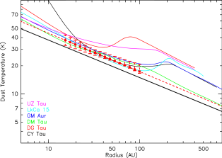
Figure 6: Temperature laws derived by Isella et al. (2009) (color curves, one for each source) compared to our assumed power law (black continuous line). The dashed red line indicate the best fit power law for DG Tau, and the error bars indicate the $\pm 1\sigma$ range in the region where this power law is constrained, i.e. about 20 to 100 AU.

However, the disk masses are sensitive to the assumed dust temperature, since they scale to first order as $1/T$. Furthermore, the dust emissivity index $\beta_{m}$ can also be affected, because the contribution of the optically thick core depends on the dust temperature. The differences in the analysis of the MWC 480 performed by Hamidouche et al. (2006) and Piétu et al. (2007) illustrate the importance of the effect. A similar effect can be seen for DG Tau in Table 9: $\beta_{m}$ changes by 0.5 between the two hypotheses on the temperature.

From the best-fit values, a few sources in our sample display partially resolved cores that may be interpreted as optically thick cores, and thus allow a direct determination of the temperature. As detailed in Appendix A, these “thick cores” satisfy two conditions: i) they have the same brightness at both wavelengths, and ii) their brightness distribution is relatively flat, because the temperature is expected to decrease as $r^{-0.4-0.7}$ at most. The fitting process indicates that this happens for DG Tau, DG Tau-b, HL Tau, T Tau, and MWC 480. The derived values are presented in Table 8. Because the Model 1 and 2 have different opacity distributions (see Fig.21-42), they predict different optically thick zones, and thus the temperature slightly depends on the assumed density model. For T Tau, the apparent difference is largely an artifact, because the source is basically a completely optically thick disk, for which the “viscous” disk model is poorly constrained. The measured values and slopes justify a posteriori our simple hypothesis for the temperature law. The dependence is small for DG Tau, DG Tau-b, and HL Tau, though. In the power law model, the extrapolated temperature at 100 AU for DG Tau is 17 K, close to our adopted value of 15 K for all other sources. HL Tau is slightly warmer, 19 K. For DG Tau-b, the temperature at 100 AU is 15 K, but the exponent is slightly lower than 0.4.

Formally, FT Tau has both a flat enough brightness distribution and a low apparent $\beta_{m}$ to be consistent with optically thick dust, but would require a very low dust temperature to match the observed flux densities. A dust temperature of 10 K at 40 AU would just provide adequate flux (the brightness can be obtained from the (apparent) opacities displayed in Fig.29). Such a low value seems inconsistent with the relatively luminous and massive central star, so the warmer, optically thin solution with $\beta_{m}\simeq 0$ is to be preferred.

Among the observed sources, MWC 480 deserves specific comments concerning the temperature. In this bright source, the “thick core” is quite large, $50-80$ AU. However, its brightness is moderate, which means that when this is interpreted as being optically thick, the derived temperatures are very low (see Piétu et al. 2006). The large size of the “thick core” results in substantial opacity corrections for $\beta_{m}$, which in turn leads to unrealistic values for Model 2.

An alternate explanation for the relatively flat brightness distribution in the inner part is a warmer, optically thin region with $\beta\simeq 0$. This is not consistent with the value of $\beta_{m}$ derived from the integrated flux, and can only happen if $\beta$ varies with radius (see Appendix A). This is studied in Sec.4.5 and MWC 480 will be rediscussed in more detail in Sec.4.6.

4.2 Surface densities

Isella et al. (2009) have published a high-resolution (0.7^′′) survey at 1.3 mm of the Taurus region, with several sources in common to our study. It has been analyzed in terms of the viscous disk model, and Table 10 shows a comparison of the results. Note that in this analysis, we assumed no inner hole for Lk Ca 15 to provide a consistent comparison, and its apparent deficit of emission in the center is purely explained by a negative value for $\gamma$. In general, our data have a higher resolution and are slightly more sensitive, which results in error bars that are lower than in Isella et al. (2009), the only exception is GM Aur, for which our resolution is moderate.

The agreement between both studies is reasonable, typically within 2 $\sigma$. The most notable exception is DG Tau. DG Tau was further studied at higher resolution by Isella et al. (2010); the agreement on $R_{t}$ is reasonable, but they find $\gamma=0.28\pm 0.05$ instead of $\gamma=1.6\pm 0.1$ in our study. The difference between the two results may be due to the widely different $uv$ coverage, linked to a non symmetric source. Our data are dominated by fairly moderate baseline lengths (up to $300k\lambda$), while Isella et al. (2010) find a substantial contribution to the imaginary part of the visibilities at 1.3 mm up to $200k\lambda$ (see their Fig.2 and image in Fig.10).

We also note that the agreement is better on $R_{c}$ (or $R_{t}$) than on $\gamma$. This is to be expected, as $R_{c}$ is a first order parameter (the radius which encloses 63 % of the disk mass), while $\gamma$ is a second-order parameter (the slope of the surface density distribution).

Table 10: Comparison with other results

Source	$R_{t}$	$\gamma$	$R_{t}$	$\gamma$
	AU		AU
	This work		Isella et al˙
CY Tau	32$\pm$ 1	0.28$\pm$ 0.06	55$\pm$ 5	-0.30$\pm$ 0.30
DG Tau	12$\pm$ 8	1.56$\pm$ 0.11	21$\pm$ 1	-0.50$\pm$ 0.20
DM Tau	86$\pm$ 5	0.54$\pm$ 0.03	86$\pm$ 32	0.80$\pm$ 0.10
LkCa 15	62$\pm$ 1	-1.24$\pm$ 0.12	60$\pm$ 4	-0.80$\pm$ 0.40
UZ Tau E	39$\pm$ 1	0.12$\pm$ 0.08	43$\pm$ 10	0.80$\pm$ 0.40
GM Aur	58$\pm$ 23	0.30$\pm$ 0.10	56$\pm$ 1	0.40$\pm$ 0.10

Rightmost columns indicate values derived by Isella et al. (2009). The leftmost columns are our results. For LkCa 15 and GM Aur, we assumed no central hole for this comparison, and thus obtain different results from those in Table 5.

4.3 Emissivity index

$\beta_{m}$ values have been reported for a number of sources in our sample by Rodmann et al. (2006) and Ricci et al. (2009). Their analysis is different from ours, because $\beta_{m}$ is derived from spatially unresolved multi-wavelength data, from a fit of the SED. Rodmann et al. (2006) use a simple power law to derive the spectral index $\alpha$ of the mm SED between 7 and 1 mm. Overall, the agreement with our results is poor, most likely as a result of several effects. First, Rodmann et al. (2006) apply a uniform correction for opacity, while we have shown that the existence of optically thick cores affect $\beta_{m}$ very inhomogeneously, with corrections ranging from 0 to 0.5. Second, the different frequency span must also affect $\beta_{m}$, because using a power law for the dust emissivity is only an approximation; in particular, the emissivity is expected to steepen at long wavelengths (e.g. Draine 2006). The agreement with the results of Ricci et al. (2009) is much better, most likely because they use a more elaborate procedure for the SED fit, in which some estimate of the disk size and surface density slope is used to account for the optical depths effects.

4.4 Individual objects

4.4.1 Multiple stars

Haro 6-10 stands out as exceptional. Although the formal fit gives marginally optically thin disks and $\beta_{m}\simeq 0$, this is likely to be an artifact caused by seeing limitation. Indeed, any small “seeing” effect spreads out a little emission and makes the source slightly more extended than in reality. This mimics an (optically thin) halo. Thus, Haro 6-10 is best represented by (two) optically thick disks of radii around 15 AU (scaling as $1/\sqrt{T_{0}}$ since only the total flux is constrained). This result indicates that the amplitude and phase calibrations are sufficiently accurate to determine sizes as small as 30 AU (total), or about $1/5^{th}$ of the synthesized beam in this case. The inclination cannot be derived for Haro 6-10. The minimum mass of each disk is $10^{-3}\,\mathrm{M_{\odot}}$ (see Appendix F, available online only).

T Tau was already studied by Hogerheijde et al. (1997) and Akeson et al. (1998) in the mm domain. As in these studies, only the northern member of the multiple system is detected. Like Haro 6-10, the emission can be explained by a nearly optically thick disk. Because of the larger size, the seeing effect is negligible and only the optically thick solution is found to be viable. Our best-fit inclination of $40\pm 4^{\circ}$ is somewhat larger than the $\sim 20^{\circ}$ derived by Ratzka et al. (2009) from IR studies. However, this only influences the apparent opacities by the ratio of the cos($i$), i.e. about 20 %. The minimum mass of the disk is $0.007\,\mathrm{M_{\odot}}$, assuming the disk is optically thick.

The quadruple system UZ Tau shows emission from two regions: one around the spectroscopic binary UZ Tau East, the other near the optically resolved wider binary UZ Tau West (separation $0.34^{\prime\prime}$ at $PA\simeq 0$, Simon et al. 1992). Given the disk inclination of UZ Tau East (Simon et al. 2000) which is confirmed by our new measurements, and assuming disks and orbits are coplanar, the true deprojected separation would be $\sim 100$ AU. Interpreting the emission around UZ Tau W as a single disk yields a similar orientation (consistent with coplanar disks) and an outer radius of $120\pm 45$ AU. This is fairly large compared to the binary separation, and may be difficult to reconcile with tidal truncation. This result, however, could be an artefact of improper subtraction of the UZ Tau East emission because any small (positive) residual emission left around UZ Tau East could bias the derivation of the position angle and size. A solution with two circumstellar disks is not totally excluded by our data. From the images, we find that the emission centroid is in between UZ Tau West A and B (see Fig.7). The displacement observed between 1.3 mm and 2.7 mm suggests that the disk around West B disk is more optically thick than that around West A. Under the interpretation of circumstellar disks, their minimum mass is $6\,10^{-4}\,\mathrm{M_{\odot}}$.

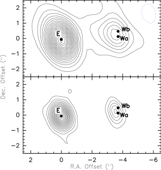
Figure 7: Relative positions of the disks and stars in the UZ Tau multiple system. The system geometry is from Simon et al. (1992), except that we used a separation smaller by 1$\sigma$ between UZ Tau-E and UZ Tau-Wa. Top: 2.7 mm map, contour step 0.9 mJy/beam (35 mK, 2 $\sigma$). Bottom: 1.3 mm map, contour step 5 mJy/beam (140 mK, 4 $\sigma$).

The small size of circumstellar disks in known binaries suggests that tidal effects are responsible for their truncation, although a firm conclusion cannot be drawn because the inclination of Haro 6-10 is unknown.

Mathieu et al. (1997) found DQ Tau to be a non-eclipsing, double-lined spectroscopic binary, comprised of two relatively equal-mass stars $M\approx 0.65\,\mathrm{M_{\odot}}$ with spectral types in the range of K7 to M1 and an orbital period of 15.804 days. The orbit is eccentric, but with an apastron around 0.28 AU, the tidal cavity should be much smaller than 1 AU. DQ Tau has been recognized as variable in the mm domain by Salter et al. (2008). The variability is caused by interactions between the magnetospheres when the two stars are near periastron, so that flares happen periodically. The observation dates and derived total flux for each date are given in Table 11. No evidence for variability is found in our data as expected, since none of our observations happened close to periastron. The measured emission is thus coming purely from the dusty (circumbinary) disk.

Table 11: Observed flux densities for DQ Tau.

Date	Frequency	Flux Density	Nearest Periastron
	(GHz)	(mJy)	(days)
1997-12-05	90	$9.6\pm 0.7$	4
1997-12-30	90	$8.5\pm 1.1$	2
1997-12-05	230	$72\pm 2$	4
1997-30-12	230	$84\pm 5$	2
2008-02-11	230	$83\pm 2^{*}$	5

(*) Long baseline data only, total flux extrapolated using the apparent size of $0.5^{\prime\prime}$ derived from the Dec 1997 data.

Another star is possibly affected by binarity: FT Tau, which displays a weak, but significant (6 $\sigma$) emission $1.3^{\prime\prime}$ west of the main star (see Fig.8), and a very small ($\simeq 60$ AU radius) disk with $\beta_{m}\simeq 0$ (see Table 5 and Fig.29). The position of the secondary peak of mm emission is, however, different from that of the near IR source found by Itoh et al. (2008).

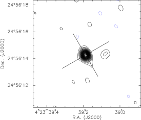
Figure 8: 1.3 mm emission from the FT Tau system showing the $\simeq 6\sigma$ detection west of the main object. Contour steps are 1 mJy/beam, or $2\sigma$.

The case of HH 30 is somehow unusual. Anglada et al. (2007) suggested that HH 30 is a binary based on the precession of its optical jet, but could not decide between a close binary and a $\simeq 15$ AU separation. Guilloteau et al. (2008) showed that the deficit of mm emission could be interpreted as a central hole consistent with the tidal truncation in the wide binary model. Here, in Model 2, the inner radius becomes unsignificant: any value below about 45 AU is acceptable for $R_{\mathrm{int}}$, because of the very steep decrease of the surface density profile for this high negative value of $\gamma\simeq-2$. In essence, this means $\gamma$ is constrained by the apparent sharp decrease of the emission near 120 AU, and not by the central deficit.

4.4.2 Sources with holes

For DM Tau, modeling the near and mid-IR SED (Calvet et al. 2005) indicates an inner hole of about 3 AU. Although this small hole is below the detectability limit of our observations, we used it in our analysis.

A deficit of emission at the center of the disk of LkCa 15 was discovered by Piétu et al. (2006), who interpreted it as a 45 AU radius hole. This central dip was also observed at lower resolution by Isella et al. (2009), but they suggested that it could be due to a negative value of $\gamma$. Our higher angular resolution data allow us to test which hypothesis best represents the observed brightness distribution. Results are reported in Table 12. The no-hole hypothesis is rejected at the $3\sigma$ level, and the best fit is obtained with an inner hole of $38\pm 4$ AU. The near-IR imaging of Thalmann et al. (2010) confirms the sharp nature of the rim of the inner hole and indicates a radius of 46 AU. The transition radius $R_{t}$ remains relatively unaffected by the presence or absence of a hole, but the value found for $\gamma$ strongly depends on the hole size: the best-fit solution is compatible with $\gamma=0$.

For GM Aur, the lack of 10 $\mu$m emission suggested a central hole of $R_{\mathrm{int}}=25$ AU (Calvet et al. 2005). The hole has also been detected in the gas traced by CO, through spectro-imaging of the J=2-1 transitions of the ¹²CO, ¹³CO, and C¹⁸O isotopologues indicating very low gas surface densities in these regions: Dutrey et al. (2008) indicate a size of $R_{\mathrm{int}}=19\pm 4$ AU. This size has been confirmed by direct imaging of the dust emission at mm wavelengths (Hughes et al. 2009). Like for DM Tau, we thus assumed $R_{\mathrm{int}}=20$ AU. The strong dependence of $\gamma$ upon the possible existence of a central hole also exists for GM Aur. Indeed, assuming no hole, we recover a very similar solution to that found by Isella et al. (2009) (see Table 10), although it is somewhat worse (near the $2\sigma$ level) than our nominal solution obtained for $R_{\mathrm{int}}=20$ AU.

Table 12: Effect of the central hole on the derived parameters for Lk Ca 15

$R_{\mathrm{int}}$	$\gamma$	$R_{c}$	$R_{t}$	$\chi^{2}$
(AU)		(AU)	(AU)
$[1]$	$-1.24\pm 0.11$	$111\pm 2$	$62\pm 2$	108674
$[46]$	$0.12\pm 0.19$	$102\pm 3$	$51\pm 2$	108679
$38\pm 4$	$-0.35\pm 0.30$	$110\pm 4$	$57\pm 2$	108664

In conclusion, with the exception of HH 30 which was discussed in Sec.4.4.1, allowing for central holes offer better solutions, and brings the surface density exponent $\gamma$ back to “standard” values between 0 and 1.5.

4.4.3 Young sources

HL Tau is a Class II object, for which the central star is not directly visible. Our measured position angle is consistent with that of the jet and of previous high-resolution studies of the mm and centimeter emission from this region (Looney et al. 2000; Anglada et al. 2007; Carrasco-González et al. 2009). The inclination of the source is more debated: early work from Cohen (1983) assumed a nearly edge-on disk, while $i=56\pm 10^{\circ}$ can be derived from the 7 mm deconvolved size from Wilner et al. (1996). Our result better agrees with the submm data obtained by Lay et al. (1997), $42\pm 5^{\circ}$, and is also consistent with the obscuration of the redshifted jet (Pyo et al. 2006). At the observed scale, the envelope that dominates the submm flux is filtered out (Looney et al. 2000). Our major finding is the substantial opacity at mm wavelengths in the inner 40 AU, which allows us to constrain the temperature, but this significant opacity does not prevent structures from becoming visible at longer wavelengths, 1.3 cm or 7 mm. Our angular resolution is insufficient to separate the possible enhancement reported near 65 AU at 1.4 mm by Welch et al. (2004) and 1.3 cm by Greaves et al. (2008), but not confirmed at 7 mm by Carrasco-González et al. (2009).

DG Tau is a bright embedded star driving an optical jet at PA 226^∘ (Eislöffel & Mundt 1998). It is surrounded by a large ¹³CO disk orthogonal to the jet (Sargent & Beckwith 1989; Kitamura et al. 1996), whose kinematics indicate a stellar mass around $0.7\leavevmode\nobreak\ \,\mathrm{M_{\odot}}$ (Testi et al. 2002). Inclinations of $45^{\circ}$ and $38^{\circ}$ are found by Pyo et al. (2003) and Eislöffel & Mundt (1998), respectively. Our measured inclination of $32\pm 3^{\circ}$ is in favor of lower values. The results quoted in Table 5 only slightly depend on the assumed orientation and inclination: $\gamma$ can be decreased by 0.1 and $R_{t}$ increased to 19 AU for the best fit orientation. The higher resolution data of Isella et al. (2010) also give lower inclinations and small (22 AU) $R_{t}$, but with a very different value for $\gamma$ (see Sec.4.2).

DG Tau-b is a young, totally obscured, star at the apex of a wide angle cavity seen in scattered light (Padgett et al. 1999). It drives an optical jet and a molecular outflow (Mitchell et al. 1997). Although the position angles derived from the jet and disk agree, we find the disk inclination to be only $64\pm 1^{\circ}$, while the jet inclination is estimated to be higher than $>75^{\circ}$ from proper motion measurements (Eislöffel & Mundt 1998). We also note that the DG Tau-b disk is best fitted with a higher flaring index $h$ than assumed for the other objects of our sample. We used $h=1.35$, for which a scale height $H_{100}=27\pm 8$ is required to reproduce the observed continuum emission. The high flaring index is consistent with the fairly flat temperature distribution ($q=0.3\pm 0.1$) also found in this source.

HERE HERE HERE

4.5 Radial dependency of the dust properties

Most previous studies assumed that the dust properties were uniform across the disk. The dual-frequency resolved images allow us to test the validity of this hypothesis, and eventually constrain the variations of dust properties as a function of radius.

4.5.1 Emissivity Index $\beta$

In Table 7 smaller transition radii $R_{t}$ are found from 2.7 mm data than from 1.3 mm data for four out of eight sources: CI Tau, CY Tau, DL Tau and DM Tau. For the other sources, the combination of sensitivity and resolution at 2.7 mm data is insufficient to distinguish. Equivalently, in the truncated power law analysis (Table 7) the slope of the surface density $p$ is systematically steeper at 2.7 mm than at 1.3 mm. A similar result was recently obtained for CQ Tau by Banzatti et al. (2010).

A possible cause for this effect is contamination by free-free emission, which adds a point-like source at lower frequencies. However, none of these sources have sufficient free-free emission to significantly contaminate the 2.7 mm flux (see Rodmann et al. (2006) for the measurements). From Rodmann et al. (2006), the contamination does not exceed $3\%$ near 2.7 mm. Removing a point source of this intensity from our 2.7 mm data does not affect our results.

Thus, the different solutions found at the two wavelengths indicate a change of dust properties, at least in the spectral index of the emissivity $\beta$, with radius. The larger $p$ and smaller $R_{t}$ at 2.7 mm than at 1.3 mm imply that the ratio of $T_{b}$(1.3mm)/$T_{b}$(2.7mm) increases with radius, hence $\beta$ increases with radius. The apparent $\beta(r)$ as a function of radius can be derived from

$$\beta(r)=\beta_{0}+\log{(\Sigma_{a}(r)/\Sigma_{b}(r))}/\log{(\nu_{a}/\nu_{b})},$$ (13)

where $\beta_{0}$ is the constant value used to derive the apparent surface densities $\Sigma_{a}(r)$ and $\Sigma_{b}(r)$ at both wavelengths, i.e. $\beta_{0}=\beta_{m}$ (see also Isella et al. (2010)).

The increase of $\beta(r)$ with radius is most easily understood in the framework of the truncated power law analysis, because it simply turns into a logarithmic dependence of $\beta(r)$ as a function of radius

$$\beta(r)=\beta_{0}+\log{((\Sigma_{a}(r/r_{0})^{-p_{a}})/(\Sigma_{b}(r/r_{0})^{-p_{b}}))}/\log{(\nu_{a}/\nu_{b})}$$ (14)

$$\beta(r)=\beta_{0}+\frac{\log{(\Sigma_{a}/\Sigma_{b})}}{\log{(\nu_{a}/\nu_{b})}}+(p_{b}-p_{a})\frac{\log{(r/r_{0})}}{\log{(\nu_{a}/\nu_{b})}}$$ (15)

$\Delta p=p(2.7\,\mathrm{mm})-p(1.3\,\mathrm{mm})$ is systematically positive in our sample (see Table 7). However, the apparent significance level is low for each source, as $\Delta p$ apparently exceeds its $2\sigma$ uncertainty in only two sources (CY Tau and DM Tau). Better constraints can be obtained by fitting the logarithmic dependence of $\beta(r)$ directly to the data

$$\beta(r)=\beta_{i}+\beta_{r}\log{(r/r_{0})}.$$ (16)

The values of $\beta_{r}$ are reported in Column 2 of Table 13 (for Model 1, but similar values are obtained for Model 2). It becomes now clear that the radial dependence is highly significant, because the weighted mean value is $\beta_{r}=0.34\pm 0.04$ (ignoring FT Tau, which has a negative $\beta$ everywhere). A Student’s T-test applied to the distribution of values of $\beta_{r}$ reported in Table 13 (including FT Tau) indicates less than 2 % chances of being compatible with $\beta_{r}=0$.

For the softened-edge model, the $\beta(r)$ function implied by Eq.13 is more complex, and an illustration of the shape of this function is given in Figure 10, which displays this apparent $\beta(r)$ for two of the sources, CI Tau and DL Tau. The hatched areas indicate the approximate range of allowed values, obtained by adding and subtracting 1 $\sigma$ to each of the parameters defining the opacity function at the two wavelengths ($R_{c}$, $\gamma$ and $\Sigma_{0}$ from Eq.5). Because some of these parameters are actually correlated, this is only an estimate of the error on the profile. The apparent index $\beta$ is large ($>1.7$) in the outer disk parts ($r>150$–$250$ AU), while it is smaller than about 0.6 near 50 AU.

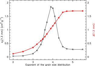
Figure 9: Dust emissivity $\kappa$ and emissivity index $\beta$ at 1.3 mm from Isella et al 2009, as a function of the exponent of the size distribution $g$.

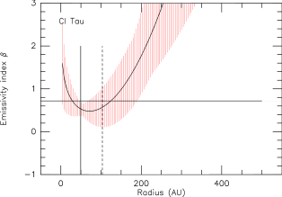
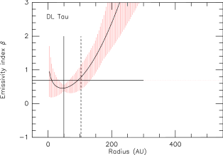
Figure 10: Apparent values of the emissivity index as a function of radius for CI Tau and DL Tau for Model 2

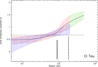
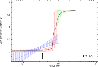
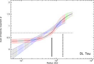
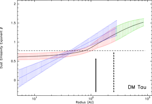
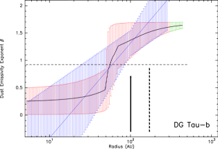
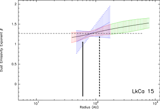
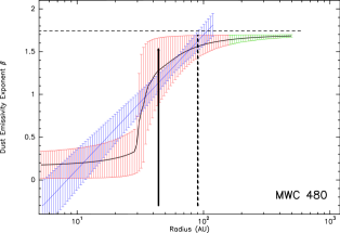
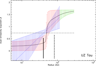
Figure 11: Constraints on the variations of the dust emissivity index $\beta$ with of radius. The red hatched area indicate the allowed range of values using the prescription of Eq.17. The blue hatched area uses the power law prescription of Eq.16 and is truncated at the outer radius found in the power law model. The thick vertical line indicates $R_{c}$, while the dashed line is $R_{t}$.

Table 13: Radial dependence of dust emissivity

(1)	(2)	(3)	(4)	(5)	(6)	(7)
Source	$\beta_{r}$	Pivot $R_{b}$ (AU)	Width $R_{w}$ (AU)	$\Delta\chi^{2}$	$R_{t}$	$\gamma$
CI Tau	$0.18\pm 0.10$	$110\pm 25$	$150\pm 90$	13	$90\pm 5$	$0.33\pm 0.04$
CY Tau	$0.32\pm 0.13$	$90\pm 10$	$5\pm 5$	17	$22\pm 1$	$0.17\pm 0.07$
DL Tau	$0.42\pm 0.07$	$90\pm 9$	$65\pm 20$	63	$75\pm 5$	$0.37\pm 0.03$
DM Tau	$0.33\pm 0.09$	$110\pm 25$	$245\pm 140$	14	$125\pm 11$	$0.48\pm 0.05$
DG Tau-b	$0.75\pm 0.31$	$60\pm 11$	$27\pm 27$	35	$72\pm 45$	$1.25\pm 0.27$
DG Tau	$0.27\pm 0.22$
FT Tau	$-0.38\pm 0.30$	$>60$		-4
LkCa 15	$0.39\pm 0.44$	$-60\pm 160$	$160\pm 360$	2
MWC 480	$0.30\pm 0.19$	$45\pm 10$	$130\pm 16$	-60	$>70$	$1.50\pm 0.10$
MWC 480	-	$36\pm 3$	$6\pm 5$	0	$41\pm 1$	$0.38\pm 0.03$
UZ Tau	$0.63\pm 0.41$	$55\pm 8$	$14\pm 26$	10	$25\pm 7$	$1.05\pm 0.25$

$\beta_{r}$ as defined in Eq.16. $R_{b}$ and $R_{w}$ as defined in Eq.17. $\Delta\chi^{2}$ is the $\chi^{2}$ offset (positive means better fit) of the fit using Eq.17 compared to the constant $\beta(r)=\beta_{m}$ hypothesis. $R_{t}$ and $\gamma$ in Col.6-7 are the parameters of the softened edge surface density distribution derived assuming the dust properties from Isella et al. (2009), see Fig.9. For MWC 480, the line in italics is under the assumption of $\kappa_{\nu}(1.3\,\mathrm{mm})=2$ cm²g^-1.

The shape of the radial dependence of $\beta$ in Fig.10, and the logarithmic dependence in Eq.16, are simple results of the choice of shape of the surface emissivity distribution, and have no physical constraints attached. In particular, apparent values of $\beta$ below 0 or above $1.7$ can result from such an analysis.

Because of the limits in angular resolution and sensitivity, some prescription of the evolution of the dust properties as a function of radius, assuming realistic conditions, must be specified to obtain better insights on the dust properties versus radius. A poor choice could make the radial dependence apparently non significant. To illustrate the problem, we used

$$\beta(r)=0.85+\frac{1.7}{\pi}\mathrm{atan}\left(\frac{r-R_{b}}{R_{w}}\right),$$ (17)

which varies between 0 (large grains) and 1.7 (small ISM-like grains). With this functional, we obtain significantly better fits, at least by $3\sigma$, but up to $8\sigma$ in DL Tau (see Table 13). Furthermore, the improvement does not depend on the assumed shape of the surface density: power laws or tapered edges yield identical results for the pivot $R_{b}$ and width $R_{w}$, although the errorbars on these parameters are typically 30% lower in the power law hypothesis. Note that there is a fairly strong correlation between $R_{b}$ and $R_{w}$, and their errorbars are in general not symmetric. To better illustrate the variations of $\beta(r)$, the resulting range of allowed values for $\beta(r)$ for each source is given in Fig.11. The logarithmic dependence found from Eq.16 is also indicated. Both functionals give approximately the same values in the regions where $\beta(r)$ is actually constrained, that is from 30 AU to the $R_{\mathrm{out}}$ of the power law. However, the log dependence fails to characterize the sharpness of the transition from low to high values of $\beta$.

Finally, although our analysis of $\beta$ excludes the flux calibration uncertainty, it is worth emphasizing that this does not affect the radial variations of $\beta(r)$, but only the mean value $\beta_{m}$. It also does not affect the relative differences in $\beta_{m}$ between sources, because all observations were made in an homogeneous way, with all spectral index measurements based on an assumed index of 0.6 for MWC 349.

4.5.2 Absorption coefficient $\kappa_{\nu}{1.3\,\mathrm{mm}}$

If grains vary in size with radius, the absorption coefficient $\kappa(\nu,r)$ will also vary. The surface density laws that were derived so far were derived assuming $\kappa(\nu,r)=\kappa(\nu_{0})(\nu/\nu_{0})^{\beta(r)}$ with $\nu_{0}=230$ GHz. In practice, there is no physical justification for any value for $\nu_{0}$, because for essentially all models of grain growth the absorption coefficient and the apparent emissivity index vary simultaneously in a more complex way. One can attempt to use a more physical approach to the grain properties, using dust absorption coefficients derived from a physical model (e.g. Draine 2006, and references therein). For example, Isella et al. (2009) (see also Natta et al. 2004) derived the absorption coefficient from a fixed grain composition, with a size distribution controlled by a single variable parameter. The size distribution is a power law with a fixed minimum and maximum radius and an exponent $g$. The absorption coefficient $\kappa$ and apparent emissivity index $\beta$ at 1.3 mm are plotted as a function of $g$ in Figure 9. From this dust model, we can derive a function $\kappa(\beta)$, which can be used in our model with the same assumptions about the radial dependency of $\beta(r)$ as previously done.

With the prescription of the opacity law described by Fig.9, and $\beta(r)$ as in Eq.17, the pivot radii $R_{t}\leavevmode\nobreak\ /\leavevmode\nobreak\ R_{c}$ are not changed very significantly. The largest changes are for CY Tau and UZ Tau, where $R_{c}$ decreases by 50%, DM Tau, where it increases by 50%, and MWC 480. Effects on $\gamma$ are negligible except for MWC 480 and UZ Tau (see Table 13). The relatively small effect on $R_{c},$ and $\gamma$ is explained because $\beta(R_{c})$ is close to 1 in most of the sources studied, and for this value $\kappa_{\nu}(230\,\mathrm{GHz})$ has an extremum. Thus the variations of $\kappa_{\nu}(r)$ around $R_{c}$ are relatively moderate, and accordingly the shape of the derived surface density is mildly affected by the radial variations of $\kappa_{\nu}(r)$.

However, these small apparent changes may be misleading, because they implicitly depend on the assumed shape of the surface density law. As $\beta(r)$ is getting close to 0 in the disk center, and thus the absorption coefficient $\kappa(1.3\,\mathrm{mm})$ could be much smaller at small radii, it is also completely possible to have a much steeper surface density gradient in the inner 40 AU. This remains hidden from our study because of the angular resolution, but also because the inner 20 – 40 AU become optically thick in some sources. If steep gradients like this exist, longer wavelength images should be able to reveal them. The strong changes observed in $R_{c},\gamma$ for MWC 480 and UZ Tau are also manifestations of this effect, although at larger scales.

In our sample, only HL Tau was studied with sufficiently high angular resolution at 7 mm and 1.3 cm to confront images with the above prediction. Although surrounded by a diffuse halo, the 7 mm image of Carrasco-González et al. (2009) is indeed very centrally peaked, but a quantitative comparison with our results is not directly possible because it displays complex structures.

4.6 MWC 480 revisited

In the simple $\beta(r)=\beta_{m}$ hypothesis, the disk of MWC 480 appears sufficiently optically thick at 230 GHz to allow the derivation of the dust temperature (Piétu et al. 2006). The optically thick region is even large enough to constrain the exponent $q$ to some extent. Leaving both $T_{0}$ and $q$ as free parameters, Model 1 and Model 2 give different best fits for the temperature, because in the best fit for Model 2, the radius at $\tau(1.3\,\mathrm{mm})=1$ is much larger (80 AU) than for Model 1 (35 AU, see Fig.39). In addition, $\beta_{m}$ is larger by about 0.3 in Model 2 than in Model 1, because the optically thick core is much larger. Furthermore, since the extrapolated temperatures in the best Model 2 are very low (7 K at 100 AU, and 2.7 K at 400 AU), the emission is no longer in the Rayleigh-Jeans domain, and $\beta_{m}$ increases because the corrections are larger at 1.3 mm than at 2.7 mm. In practice, Model 2 finds a low temperature with a steep exponent ($\simeq 0.6$) because of two effects: i) the brightness is identical at 2.7 mm and 1.3 mm in the inner 40 AU, and ii) the imposed shape of the surface density is too flat in the inner 80 – 100 AU (in order to provide sufficient opacities beyond 100 AU). To account for these two constraints, an optically thick core of 80 AU is fitted, with a steeply decreasing temperature. High temperatures can only be found by allowing the surface density to fall faster than Model 2 allows between 40 and 80 AU.

Clearly, in this case, although low temperatures are needed in the inner regions, extrapolating the same power law introduces non-physical biases on the disk mass and on $\beta_{m}$. Leveling the temperature to a minimum value of 12 K beyond 45 AU provides a better fit to the observations, and allows us to bring back $\beta$ below 2. This may be an indication of the temperature rise with radius that is expected to begin when the opacity for re-emission drops below 1. However, the very low apparent temperatures in this object are surprising because of the luminous central star. This may be linked to the geometry of that source. From its IR SED, MWC 480 is a Group II Ae disk, which is interpreted as a self-shadowed disk with small flaring (Meeus et al. 2001). Indeed, it has never been detected in scattered light, despite a fairly favorable inclination. Yet, the temperature derived from ¹³CO is $\simeq 23$ K at 100 AU, with an exponent $q=0.4\pm 0.1$ (Piétu et al. 2007), and if the disk remains optically thick even at 3 mm, we would expect dust and gas to be thermalized at the same temperature.

Allowing $\beta(r)$ to change with radius also offers a much more attractive solution to the continuum emission of MWC 480. The flattening of the emission in the inner 50-80 AU is no longer ascribed to an optically thick core at low temperatures, but to a flattening of the surface density distribution, while the ratio of 2.7 to 1.3 mm emission is matched by allowing $\beta(r)$ to become small in the inner 30 AU. Although it is equivalent in $\chi^{2}$ to the constant $\beta(r)=\beta_{m}$ solution, this new model agrees with less extreme dust temperatures. In fact, the dust emission is largely optically thin in this case, and there is a substantial degeneracy between the dust temperature and the derived disk mass / surface density. A lower limit to the dust temperature at 100 AU is 23 K (assuming $q=0.4$), which is consistent with the temperature derived from ¹³CO line emission by Piétu et al. (2007). This lower limit was used to derive the surface density.

If we use $\kappa(\beta)$ as implied in Fig.9, the fit quality is slightly degraded, but most importantly, the derived shape for the surface density and the temperature profile are significantly affected (see Table 13). We find $\gamma\simeq 1.5$, and a large transition radius $R_{t}>70$ AU, much like for GM Aur. The best-fit temperature profile is flat, $q=0.0\pm 0.1$, with $T>25$ K. The higher $\chi^{2}$ value derived under these assumptions may be related to an oversimplified temperature profile, as in the simpler analysis $q\simeq 0.5$ was found in the inner regions.

5 Discussion

5.1 Dust properties

From the above results, we find large grains ($\beta<0.5$) in the inner 60 to 100 AU, and small grains beyond for seven sources (CI Tau, CY Tau, DL Tau, DM Tau, DG Tau-b, MWC,480 and UZ Tau-E). Two other sources in our sample have very low $\beta$: the FT Tau disk is truncated at 60 AU, while DQ Tau has not been observed with sufficient resolution at 2.7 mm, so that $\beta(r)$ is not constrained in the outer regions. A third source may have low $\beta$ up to 60 AU: T Tau N, although we interpreted it as being optically thick. On the other hand, $\beta$ is not constrained in the inner region for the two other sources observed with sufficiently high resolution in our sample, because in DG Tau, the inner 50 AU may be optically thick, while for LkCa 15, the inner 50 AU are (largely) devoid of dust. For HH 30 we find a low $\beta$ below 120 AU, while it is known from the scattered light images that small grains exist at least up to 250 AU or even 430 AU (Burrows et al. 1996), the outer radius of the gas distribution (Pety et al. 2006). Finally, in HL Tau, large grains exist in the inner 20 AU, as shown by the 1.3 cm and 7 mm images (Carrasco-González et al. 2009). Thus, in essence, all sources in our high-resolution sample show large grains (low $\beta$) below 100 AU and small grains beyond, although the detailed shape of the radial dependence cannot be characterized by our data.

The apparent variations of $p$ with wavelength observed by (Banzatti et al. 2010) for CQ Tau also points out towards an increase of $\beta(r)$ with radius in that source. Moreover, although they considered it to be insignificant, the same trend is found in RY Tau and DG Tau by Isella et al. (2010). Thus, the radial dependency of $\beta(r)$ appears to be a general property of disks.

Our findings that $\beta$ is low in the inner 60 to 100 AU of all disks in which we can constrain the radial dependency also sheds new light on the results quoted by Ricci et al. (2009). Ricci et al. (2009) found a lower average value for the spectral index $\alpha$ for disks with low 1.3 mm flux than in disks that show strong emission. A possible interpretation is that these weaker disks are optically thick and very small, like those surrounding the binary Haro 6-10. These weak disks may just miss the extended, low brightness parts with high values of $\beta$ that we found in bright sources. In our sample, a clear example for this behaviour is FT Tau. Given our measured $R_{b}$, a testable prediction is that these faint disks should be smaller than about 100 AU in radius. Note that this does not address the origin of the small size for these disks, although tidal truncation is an obvious candidate. On the other hand, in AB Aur, which has an inner hole around 100 AU (Piétu et al. 2005), the mm emission is coming from the small grain regions, which results in a mean $\beta_{m}=1.4\pm 0.2$, which is different from all other sources. Such a high $\beta_{m}$ is not an indication of different grain growth in this source, but just a side effect of the radial dust distribution. We further stress that the $\beta_{m}$ values derived in all previous analyses represent an ill-defined average over the disk structure.

5.2 The shape of the surface density distribution

Given the high resolution and sensitivity, can we decide which model fits the data better? The lowest $\chi^{2}$ is the usual indicator, but care must be taken that the $\chi^{2}$ is not affected by different biases between the two models owing to numerical effects in the model computation. The precision required for this is always higher than the precision required to obtained converged parameters and errors within a given model, because the discretization effects impact models differently (see Appendix B, available online only). For the models considered, the problem is somewhat relaxed because they both derive from a generic one (see Eq.5). We nevertheless checked by using oversampled grids that the $\chi^{2}$ results were converged.

From Table 5, the softened-edge model does not appear superior to the power law model to represent the observations. In this process, the compact optically thick sources should be ignored. For these sources, the data are insensitive to the true shape, but can be significantly affected by small instrumental effects. For example, the seeing that results in flux spreading because of atmospheric phase variations tends to produce a small halo around the compact core. In our sample of 23 individual objects, this may affect five sources. Of the remaining objects, four sources are best represented by a power law: DG Tau, DQ Tau, HL Tau and (marginally) DM Tau. On the other hand, six sources are better fitted by the exponential-edge model: CI Tau, CY Tau, DL Tau, UZ Tau E, and marginally LkCa 15. Both models fit equally well the last seven sources, which were observed with lower angular resolutions except for DG Tau b.

Despite the high resolution (projected baselines above $500k\lambda$) and sensitivity, the shape of the surface density remains difficult to constrain. The truncated power law was initially used because it provides the simplest parametric model. It is furthermore not linked to any specific physical disk model, a property which can be seen either as an advantage (by providing no specific bias) or handicap (as having no physical ground). Its principal failure was its inability to represent continuum and spectral line emission with the same outer radii (Piétu et al. 2007). The softened-edge model has recently gained favor because, as suggested by Hughes et al. (2008), it may provide a framework that can explain both the continuum and optically thick CO emission. The exponential taper is often referred to as having a physical background, because viscosity is expected to spread out initially small disks. However, the exponential taper is only a specific solution of self-similar evolution of a viscous disk with a power law distribution of the viscosity (with a constant in time exponent). In practice, self-similarity and time independence are unlikely to strictly apply to real disks, so the resulting specific shape is also an approximation. Any core+halo structure would essentially yield the same result, provided the halo is just dense enough to explain the molecular emission, but tenuous enough to have little continuum emission from dust. This core+halo structure was invoked by Dutrey et al. (1994) and Guilloteau et al. (1999) to interpret the circumbinary environment of GG Tau.

In the strict framework of a viscous disk model, we find values of $\gamma$ that are somewhat larger (and with higher dispersion) than those derived in the previous studies by Isella et al. (2009) and Andrews et al. (2009). The discovery of a radial dependence of the dust properties brings additional complexity to the problem. Clearly, the surface density of the gas is not well traced by the continuum emission at a specific frequency in this picture. It all depends on how the dust emissivity $\kappa(\nu,r)$ changes as a function of radius, so that the derived $\gamma$ is expected to depend on the assumed dust properties.

It is also important to realize that the derived dust masses of the disk may be significantly affected by the variations of the dust properties with radius. Table 14 indicates the disk masses obtained for Model 2 using Eq.17 with the two different hypotheses on the dust absorption coefficient ($\kappa_{\nu}$(1.3 mm) constant or tied to $\beta(r)$ as from Fig.9). In our sample, although the effect is small for the other sources (about 20 %), the masses of the CY Tau and DM Tau disks are strongly modified when using the dust properties from Isella et al. (2009). In particular, the mass of the DM Tau disk becomes quite significant (0.2 $\,\mathrm{M_{\odot}}$) compared to the stellar mass (0.5 $\,\mathrm{M_{\odot}}$ Dartois et al. 2003). Such a large mass would have significant effect on the rotation curve of the gas, while it is known to be Keplerian with high accuracy (velocity exponent $0.50\pm 0.01$, Piétu et al. 2007).

Table 14: Disk masses with variable dust properties

Source	$M_{c}$ ($10^{-3}$ $\,\mathrm{M_{\odot}}$)	$M_{v}$ ($10^{-3}$ $\,\mathrm{M_{\odot}}$)	Ratio
CI Tau	43 $\pm$ 4	51 $\pm$ 5	1.18$\pm$ 0.18
CY Tau	18 $\pm$ 1	46 $\pm$ 2	2.52$\pm$ 0.09
DG Tau	36 $\pm$ 5	42 $\pm$ 6	1.18$\pm$ 0.27
DG Tau-b	151 $\pm$ 59	179 $\pm$ 60	1.19$\pm$ 0.73
DL Tau	51 $\pm$ 1	60 $\pm$ 1	1.18$\pm$ 0.04
DM Tau	32 $\pm$ 8	192 $\pm$ 49	6.07$\pm$ 0.52
UZ Tau	24 $\pm$ 1	32 $\pm$ 2	1.33$\pm$ 0.14

$M_{c}$ is the disk mass for Model 2 (tapered edge) for $\kappa(1.3\mathrm{mm})=2$ cm².g^-1, while $M_{v}$ is for $\kappa(1.3\mathrm{mm})$ as in Fig.9. A gas-to-dust ratio of 100 was assumed. Ratio = $M_{c}/M_{v}$.

This result is under the assumption of a “normal” gas-to-dust ratio of 100. However, the gas-to-dust ratio itself is expected to change as a function of time and radius in the disk. For DM Tau, the potentially large dust mass suggests that the gas-to-dust ratio must be decreased. Molecular tracers may help to constrain the gas surface density more directly, but then a good understanding of the chemistry is required to recover the hydrogen content from the (very few) trace molecules that display strong enough lines to be observable: CO and its isotopologue ¹³CO, HCO⁺, CN, HCN, CS and H₂CO (Dutrey et al. 1997).

A simpler alternative is that the adopted dust properties are inappropriate. For example, with similar grain size distributions, but using a different dust composition (in particular porous grains), Ricci et al. (2009) derive dust opacities on the order of $3-20$ cm².g^-1 instead of $0.4-2$ cm².g^-1 from Isella et al. (2009). The overall dependencies of $\kappa$ and $\beta$ upon the grain size distribution display the same characteristic behavior. Note, however, that it is possible to obtain $\beta$ values above 2, provided the grain size distribution as a relatively steep cutoff near $a_{+}=\lambda/2\pi$, i.e. about 0.5 mm for $\lambda=3$ mm, because the emissivity of a grain size $a$ has a pronounced maximum at wavelengths $\sim 2\pi a$ (see e.g. Natta et al. 2004), before dropping as $1/a$ at longer wavelengths. In the following, we scale down the surface densities of sources analyzed with radial dust opacity gradients by a factor 3, to avoid a different bias in the comparison with sources for which this analysis was not possible.

Figure 12 displays the resulting surface densities (of gas+dust) for the sources in the sample. Uncertainties were omitted for clarity in this figure, but can be recovered from the Figs.21-42. We note that the younger sources have higher surface densities in the inner 50 AU than other objects. They are also more centrally peaked, on average. This picture is qualitatively similar to the predictions from viscous disk evolution.

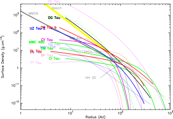
Figure 12: Surface densities of observed sources. Thick lines are for sources in which a variation of $\beta$ and thus $\kappa$ with radius was derived. Thin lines are for sources for which we assumed $\kappa(1.3\,\mathrm{mm}=2$ cm².g^-1. The gray line is the MMSN, while the yellow area indicates the Solar Nebula from Desch (2007).

Figure 12 also displays the profiles derived for the Solar Nebula, the MMSN (Hayashi 1981, gray line) and the solution proposed by Desch (2007), which accounts for the early planet migration as proposed by the Nice model (Tsiganis et al. 2005; Gomes et al. 2005) (yellow range). The solution proposed by Desch (2007) (see Appendix E, available online only) for the Solar Nebula is a steady-state solution, which allows for sufficient time (few Myr) for the giant planets to reach isolation mass. In comparing with our results, it is important to realize that our observations constrain essentially the slope and surface density between 50 to 150 AU, while the other regions are obtained by extrapolation of the analytically prescribed shape. In our sample, only the youngest objects have sufficiently high surface densities to be compatible with the MMSN.

5.3 Towards an evolutionary model ?

5.3.1 Viscous evolution of the gas disk

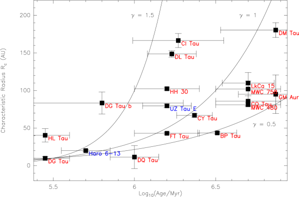
Figure 13: Characteristic radius $R_{c}$ (in AU) as a function of estimated stellar ages (in Log₁₀ of $10^{6}$ years).

Figure 13 displays the characteristic radius $R_{c}$ as a function of estimated stellar ages. The figure apparently suggests an increase of $R_{c}$ with age. Performing a Spearman rank-order correlation test indicates a correlation coefficient of 0.60, and a small probability of random distribution (0.7 % only). This correlation study does not include the error bars on age and $R_{c}$, however. Furthermore, the correlation coefficient is heavily influenced by the two youngest objects, DG Tau and HL Tau and the two oldest ones, GM Aur and DM Tau, all sources for which the power law model gives a better fit than the softened-edge model. Nevertheless, taken at face value, our data seem to confirm the trend suggested by Isella et al. (2009), which they have interpreted as evidence for the viscous evolution of disks.

Figure 14: Initial disk radii (AU).

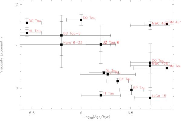
Figure 15: Surface density exponent $\gamma$ as a function of estimated stellar ages (in Log₁₀ of $10^{6}$ years).

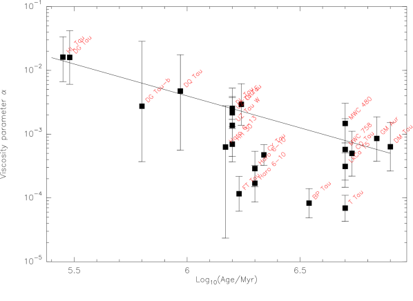
Figure 16: $\alpha$ parameter as a function of estimated stellar ages.

In the framework of self-similar viscous evolution, the surface density depends on five intrinsic parameters: a normalization constant $C$, the initial disk radius $R_{1}$, a normalized age $T$, the viscosity $\nu_{1}$ at radius $R_{1}$ and its radial exponent $\gamma$. We have three measurements from our study ($M_{d}\leavevmode\nobreak\ \mathrm{or}\leavevmode\nobreak\ \Sigma_{0},R_{c},\gamma$), the stellar age $t_{*}$ from evolutionary tracks as quoted in Table 1, and the mass accretion $\dot{M}$, usually derived from the accretion luminosity (Gullbring et al. 1998). Appendix D (available online only) details the relationship between these observable quantities and the primary parameters of the radial surface density evolution.

A perfect correlation between disk sizes and age is not expected. The initial characteristic sizes of disks will add significant scatter. In this respect, the most significant fact is perhaps the envelope of allowed $R_{c}$ versus ages, which places an upper limit on these initial sizes. This limit is related to the initial specific angular momentum. Larger disks would fragment and lead to binary and/or multiple systems. In this respect, it may be relevant that the young object with the largest $R_{c}$ is UZ Tau E, a spectroscopic binary member of a hierarchical quadruple system. Another source of scatter resides in the exponent of the viscosity $\gamma$. Fig.13 displays evolutionary curves of $R_{c}=R_{1}T^{1/(2-\gamma})$ for three values of $\gamma$, starting with a common initial radius $R_{1}=10$ AU (see Appendix Eq.25 for a derivation of the evolution of $R_{c}$ versus time). Although the extreme values of $\gamma=0.5$ and $1.5$ appear, at first glance, to provide a good fit to the envelope of the distribution of $R_{c}$ versus ages, the actual picture is more complex. In particular, a number of stars close to the $\gamma=0.5$ curve have in fact $\gamma=1.5$ from our data set, while the reverse is also true.

The viscous timescale is given by (see Eq.32)

$$t_{*}+t_{s}=\frac{M_{d}}{2(2-\gamma)\dot{M}}.$$

Unfortunately, because the stellar ages $t_{*}$ are very uncertain and we expect in general $t_{s}\ll t_{*}$, $t_{s}$ remains largely unconstrained by the observations. Rather, Eq.32 provides a loose constraint on the allowed range of disk masses and ages. An alternate way to constrain the viscous timescale is to look at the younger objects, for which the viscous evolution may not have had time to erase the initial conditions. In our sample, younger objects are better represented by power laws. This suggests that young disks are still influenced by the history of infall from the original proto-stellar cloud, and that the viscous timescale is on the order of a few $10^{5}$ years, the age of these youngest objects.

With this rough estimate for $t_{s}$, we can in principle derive $T$ and recover the distribution of $R_{1}$ in our sample from Eq.25, but the propagation of errors leads to large uncertainties (see Fig.14). This is to be expected, because the viscous evolution has largely erased the memory of the initial conditions.

Self-similarity would also imply that the exponent $\gamma$ remains constant over age. The distribution of $\gamma$ vs age is given in Fig.15. Our distributions of $\gamma$ are somewhat different from those derived by Andrews et al. (2009) and Isella et al. (2009). The former is centrally peaked around 0.9. The latter exhibits values lower than 0.8; however, we have argued in Sec.4.4.2 that some of the derived values are affected by the interpretation of the central deficit of emission. In our sample, although there is no obvious correlation, stars of ages 1-3 Myr have on average lower $\gamma$ ($\simeq 0.3$) than either younger or older objects. Note that from Eq.28, for $\gamma=1.5$, we expect $\dot{M}(t)\propto t^{-2}$ in good overall agreement with the empirical relation found by Hartmann et al. (1998). On the other hand, $\gamma=0.5$, which corresponds to the so-called $\beta$ prescription of the turbulence (see Appendix E for details), yields $\dot{M}(t)\propto t^{-4/3}$ only, somewhat too small to explain Hartmann et al. (1998) correlation. Note however that large values of $\gamma$ are unlikely to apply to the whole lifetime of the disks: if we assume $\gamma$ has been constant with time, the two old disks with large $\gamma$ (GM Aur and MWC 480) would have started with exceptionally small radii ($<2$ AU, see Fig.14). Thus, invoking some evolution of the viscosity exponent with age seems required.

An alternate vision on the viscosity is to look at its value at some arbitrary fixed radius, for example at $R_{100}=100$ AU. Using the $\alpha$ prescription of the viscosity, the $\alpha$ parameter at 100 AU is given by (Eq.38)

$$\alpha(R_{100})=\frac{R_{c}^{(2-\gamma)}R_{100}^{\gamma}}{3(2-\gamma)^{2}c_{s}(R_{100})H(R_{100})t_{*}},$$ (18)

where $c_{s}H$ scales as $(L_{*}/M_{*}^{2})^{1/4}$ to first order (see Appendix D for the derivation). Using $L_{*}/M_{*}^{2}$ from Table 1, and our adopted values of $T_{g}=15$ K and $H=16$ AU at 100 AU for the median value of $L/M^{2}=3\,\mathrm{L_{\odot}}/\,\mathrm{M_{\odot}}^{2}$, the resulting $\alpha$ are displayed in Fig.16. There is substantial scatter, but the measurements suggest an overall decrease of $\alpha$ versus time, roughly as $1/t_{*}$.

5.3.2 Evolution of the dust

The radial dependence of $\beta(r)$ and the behavior of $R_{c}$ as a function age may be understood in a more complex scheme where viscous spreading plays a significant role. Indeed, only small dust grains are efficiently coupled to the gas, while the larger ones should drift quickly inward (e.g. Weidenschilling 1977). Hence, one naturally expects that large grains will remain confined to the inner regions, which leads to an apparent increase of $\beta(r)$ with radius. Simulations of the grain-growth, dust-gas coupling and fragmentation processes have been performed by Brauer et al. (2008), and further expanded by Birnstiel et al. (2010a) to include the disk accretion phase and viscous evolution. There is no specific prediction for the evolution of the shape of the grain size distribution with radius which could be compared to our data. However, from Fig.10 of Birnstiel et al. (2010a), the smaller grains have outward net velocities beyond about 80 AU. A similar result was found by Garaud (2007), although her approach neglects the fragmentation processes. This radius is similar to the transition radius between low and high values of the emissivity exponent $\beta$ found in our study.

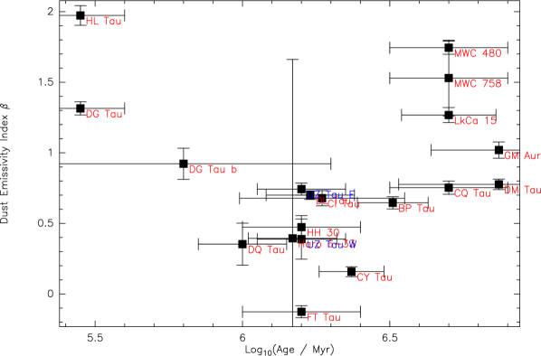
Figure 17: Dust opacity index $\beta_{m}$ as a function of estimated stellar ages.

Despite being a rather ill-defined quantity, the average $\beta_{m}$ has been used to characterize disks in most previous studies. Figure 17 displays $\beta_{m}$ as a function of estimated stellar ages. Very young sources have high values of $\beta_{m}$, comparable to the value found for ISM grains, which could indicate that the dust grains have not yet significantly evolved in these objects, at least at the characteristic distances that we sample in these sources (100 – 300 AU). Typical T Tauri disks have $\beta_{m}<0.7$, which indicates significant grain growth. However, we also find that the older disks display high values of $\beta_{m}$ too, well above the characteristic value for the “middle-aged” T Tauri stars. The radial dependency of $\beta$ provides an explanation for this distribution of average $\beta_{m}$ with stellar ages. As disks get larger with time, the apparent average $\beta_{m}$ increases, which leads to the secondary increase of $\beta_{m}$ for older objects as shown in Fig.17.

Birnstiel et al. (2010b) evaluate the effect of the grain growth and fragmentation on the apparent spectral index $\alpha_{1-3\mathrm{mm}}$ for disk masses ranging from 0.005 to 0.1 $\,\mathrm{M_{\odot}}$  and compared them to the observed distribution obtained by Ricci et al. (2009). They use a fixed disk model with $R_{c}=60$ AU and $\gamma=1$. The growth and fragmentation model predicts an increase of $\beta(r)$ at radii ranging from 40 to 100 AU (their Fig.3), which broadly agrees with our finding. However, in their analysis the distribution of average $\alpha_{1-3\mathrm{mm}}$ vs observed 1.3 mm flux density only roughly matches the strongest sources. This effect is related to the dependence of the “fragmentation barrier” grain size on the surface density: less massive disks are expected to have smaller grains, and thus larger $\alpha_{1-3\mathrm{mm}}$. As mentioned in Sec.5.1, a simple way to provide a better agreement with the data is to assume that the faint disks are actually not less dense than the strong ones, but truncated to smaller sizes. In this case, $\alpha_{1-3\mathrm{mm}}$ is expected to decrease with source flux because of the radial dependence of $\beta(r)$.

Finally, the discussion of the viscous properties of the disk presented in Section 5.3.1 used $\gamma$ and $R_{c}$ derived from the dust content, i.e. they implicitly assume a constant dust-to-gas ratio. In reality, the dust-to-gas ratio is expected to change with radius because of the concurrent effects of accretion, viscous spreading, grain drift, growth and fragmentation. In general, it is expected to decrease with radius, because the coupling between dust and gas increases with density, see for example Fig.6 of Birnstiel et al. (2010a). The average dust-to-gas ratio is also expected to decrease with time, as the largest particles are drifting inward, being eventually advected onto larger bodies, either embryos or the central star. Accordingly, the discussion on possible changes of viscosity ($\alpha$ parameter and/or $\gamma$) presented in Section 5.3.1 should be taken with some additional care.

6 Conclusions

We report here the results of the first dual-frequency and high-resolution study of dust disks in the mm domain where the dust is mostly optically thin.

• Independent data sets allowed us to verify the robustness of the derived parameters and of their error bars. The geometric parameters (inclination and orientation) agree well with determinations from other constraints, such as scattered light images, optical jets, and the Keplerian rotation of the disks.

• We derived proper motions for 10 sources in our sample.

• Tidal truncation is found to affect the disk sizes in binary systems.

• Despite the combination of high angular resolution and sensitivity, we found that the viscous disk model does not generally provide a significantly better fit of the continuum data only than the simple truncated power law description. Baselines well above 300 k$\lambda$ are required to distinguish between these two descriptions. In very young sources, the simple power law model appears to work somewhat better, while the exponential edge is marginally better for evolved objects.

• Inner holes also appear to provide a better explanation than negative values of $\gamma$ for sources showing a deficit of emission at the center like GM Aur and LkCa 15.

• We have strong evidence for radial dependence of the dust emissivity exponent $\beta$ with radius. In all cases, $\beta$ is found to increase with radius, i.e. we find grain size which decreases with distance from the star. High $\beta$ values (1.7 –2, typical for ISM grains, or even possibly higher) are found beyond 100 AU, while the inner regions may display values down to nearly 0. This result is obtained whatever disk model has been adopted (surface density shape and temperature profile).

• We have possible evidence for optically thick cores in a few sources, which provide a direct estimate of the temperature of large grains. However, in some cases, inner regions with $\beta=0$ may be misinterpreted as thick cores at low temperatures.

• Despite the ambiguities introduced by the variable dust properties, the characteristic size of the disk appears to increase with stellar ages, which broadly agrees with the viscous evolution. A more detailed comparison with the models suggests a decrease of the $\alpha$ viscosity parameter with time, as well as changes in the exponent of the viscosity.

These observations provide the first evidence for the expected effect of the dust grain evolution in circumstellar disks resulting from grain growth, fragmentation and, viscous transport. The comparison with model predictions is limited by the angular resolution obtained at the longest wavelengths, about 100 AU, which requires some parametric approach to constrain the radial dependence of $\beta(r)$ (and by inference, $\kappa(r)$ using some specific dust model). With the advent of ALMA and e-VLA, a direct inversion of the $\beta(r)$ profile at linear resolutions of order 10-20 AU will become possible, enabling us to derive much more accurate constraints on the dust properties as a function of radius. This will be possible not only using two wavelengths as here, but over more than a decade in frequency.

Appendix A Optical depth vs variable $\beta$

Figure 18: Sample result illustrating the shape of the brightness distribution for our disk models. Thick line: constant $\beta$ power law model at 1.3 mm, dashed line: same model at 2.7 mm. Dotted line: constant $\kappa$(1.3 mm) but variable $\beta(r)$, tapered-edge model at 1.3 mm; dash-dotted line: same model at 2.7 mm.

Because a direct inversion of the brightness temperature profile is impossible, the determination of the parameters is fully implicit. Figure 18 illustrates two possible types of brightness temperature profiles that can occur in our analysis. The continuous and dashed lines represent brightness at 1.3 mm and 2.7 mm for a typical power law distribution, with constant dust properties $\beta(r)=\beta_{m}$. The outer region is optically thin, and the slope constrains $p+q$. $\beta_{m}$ is derived from the brightness ratio $O$. The inner region is optically thick, and constrains the exponent $q$ as well as the temperature at 20 AU, $T_{20}$. The small brightness difference between the two frequencies is caused by the Rayleigh-Jeans correction. The dotted and dot-dashed lines represent an optically thinner disk at 1.3  and 2.7 mm respectively, with a viscous type profile with $R_{c}=150$ AU. In addition, $\beta(r)$ is assumed to vary with radius following Eq.17 with $R_{b}=60$ AU and $R_{w}=20$ AU, $\kappa$(1.3 mm) being constant. Here, the inner region is optically thin, and its slope is $q+\gamma$. Note that if the temperature of that disk would be 4 times higher, it would mimic reasonably well the previous power law, optically thick case, provided $\gamma$ is not too large. Accordingly, sources displaying a wavelength-independent flattened (apparent exponent $\simeq 0.4--0.7$) inner brightness distribution can be interpreted either as optically thick sources, or as variable $\beta(r)$ with $\beta(r)\simeq 0$ in the inner region. Steeper apparent exponents are not realistic for the temperature dependence. Note that the typical noise level is around 0.05 – 0.1 K in our observations at both wavelengths.

Appendix B Sampling effects and best model

Because of the fully implicit derivation of the model parameters, an objective determination of the “best” model is difficult. The same source may be (nearly) equally well represented by either Model 1 or Model 2. We use a $\chi^{2}$ criterium to determine the best matching model. However, it is important to realize that our data consists in a large (several $10^{4}$) number of statistically independent visibilities, each with very little (essentially zero) signal-to-noise. The $\chi^{2}$ is given by

$$\chi^{2}=\Sigma(O_{i}-M_{i})^{2}*W_{i},$$ (19)

where $O_{i}$ are the (complex) observed visibilities ($O^{2}$ actually being used to note $O\times O^{*}$, $O^{*}$ being the complex conjugate of $O$), $M_{i}$ the modeled visibilities. The weights $W_{i}=1/\sigma_{i}^{2}$ are derived from the theoretical noise using the system temperature, antenna gain, observing bandwidth and integration time. In general, $\sigma_{i}>>M^{b}_{i}$, where $M^{b}$ is the best-fit model, so even the null model $M_{i}=0$ yields a $\chi^{2}$ on the order of $N$, the number of visibilities, as $W_{i}$ is the inverse of the variance of $O_{i}-M^{b}_{i}$. Thus, the reduced $\chi^{2}$, $\chi^{2}_{r}=\chi^{2}/N$ is a poor evaluation of the fit quality, which is close to 1 even for a very poor (null) model. Only the relative differences $\Delta\chi^{2}$ between models of equivalent number of parameters can reveal whether one is better than the other.

Another subtle effect in comparing absolute values of $\chi^{2}$ is the impact of discretization. A numerical model $M$ is an approximation of the theoretical model $T$, $M=T+E$, where $E$ is a numerical error term. So

$$\chi^{2} = \Sigma(O_{i}-M_{i})^{2}W_{i}$$ (20)

$$= \Sigma(O_{i}-T_{i})^{2}W_{i}+\Sigma E_{i}^{2}W_{i}-2\Sigma E_{i}(O_{i}-T_{i})W_{i}.$$ (21)

Because the model fit the observations and the numerical errors are not correlated with the observations, the last term is negligible, consequently the final $\chi^{2}$ is a sum of the true (no numerical errors) term plus an offset cause by numerical effects. To make numerical errors negligible requires $\Sigma_{i}E_{i}^{2}W_{i}$ to be much less than 1. This is especially important when comparing different theoretical models. However, within a given model, the best-fit parameters may be determined with sufficient precision even if the numerical error term is not small.

Appendix C Impact of the assumed temperature law

In this appendix, we investigate the impact of the dust temperature profile on the derived disk parameters. We consider two different profiles. Profile (i) is a power law $T(r)=T_{100}(r/100\mathrm{AU})^{-q}$. Profile (ii) is a broken power law: it has a constant temperature between $R_{i}=40$ AU and $R_{f}$, $R_{f}$ being a variable parameter, while for $r<R_{i}$ or $r>R_{f}$, the temperature is a power law with exponent q=0.5, with to $T(r)=T_{1}$ at $r=1$ AU. The temperature law is continuous as a function of $r$, and we used $T_{1}=200$ K by default. We analyzed the observations of a few sources (DL Tau, DM Tau and MWC 480) to explore the dependency of the derived surface density parameters on $T_{0},q$ and $R_{f}$. Figure 19 illustrates the main impact of the temperature law on the surface density parameters, which is applicable to all optically thin sources. Figure 19 is for Model 2 (so $p$ is to be interpreted as $\gamma$), but similar results are obtained for Model 1.

For Profile (i) :
- $\Sigma_{0}$ is nearly proportional to 1/T, with small corrections at low T owing to deviations from the Rayleigh-Jeans behavior.
- Similarly, $p+q$ is nearly constant. This is equally valid for Model 1 (power law) and Model 2 (tapered edge).
- In Model 1, $R_{\mathrm{out}}$ is only weakly affected by the changes in $p$
- In Model 2, $R_{c}$ increases by 20 to 30 % when $q$ increases from 0 to 0.5.

For Profile (ii) :
- In Model 1, $R_{\mathrm{out}}$ slightly decreases with $R_{t}$ (by about 10 %), and $p$ changes by about 0.1. Variations are not fully monotonic, however.
- In Model 2, $R_{c}$ decreases by about 20 to 30 %, when $R_{t}$ goes from 50 to 200 AU. This is similar to the effect of $q$ in Profile (i), as increasing $R_{t}$ flattens the temperature distribution.

For more optically thick sources, like MWC 480, the effect on $p$ is larger, because of the opacity corrections. However, in this case, $q$ can be determined from the observations, because the $\chi^{2}$ significantly depends on its value. Restricting the range of $q$ to within its typical uncertainty limits the impact on $p$ to about 0.2.

Except for the absolute scaling of the density as $1/T_{100}$ (or $1/T_{1}$ in Profile (ii)), the derived density distribution are thus not significantly affected by the assumed temperature law.

More importantly, $R_{c}$ and $p$ are affected in the same proportions at both wavelengths. Thus, the uncertainties on the temperature law have no significant effect on the derivation of the radial dependence of $\beta(r)$ (see Figure 20). Incidentally, we note that in DL Tau, a better fit to the observations is obtained using Profile (ii) with $R_{f}=100$ AU.

Figure 19: Sample results illustrating the main dependency of the surface density profile on the temperature law. Top left: $R_{c}$ versus $q$. Top right: $R_{c}$ versus $R_{f}$; bottom left: $\Sigma.T$ verus $T$; bottom right: $p+q$ versus $q$. The observed source is DL Tau.

Figure 20: Sample results illustrating the weak dependency of the dust parameters $R_{b}$ and $R_{w}$ on the assumed temperature law.

Appendix D Disk parameters from observable quantities in the viscous model

The shape of the surface density profile used in Model 2 corresponds to the self-similar solution of the viscous evolution of a disk under the assumption that the viscosity is constant in time and a power law of radius (see Lynden-Bell & Pringle 1974; Pringle 1981). Under these assumptions, the surface density as a function of time and radius is given by (Eq.17 of Hartmann et al. (1998))

$$\Sigma(R,t)=\frac{C}{3\pi\nu_{1}r^{\gamma}}T^{-(5/2-\gamma)/(2-\gamma)}\exp\left(-\frac{r^{(2-\gamma)}}{T}\right),$$ (22)

where $r=R/R_{1}$, $T=(1+t_{*}/t_{s})$ is a dimensionless time, $t_{*}$ the disk/star age and $t_{s}$ is the viscous timescale at $R_{1}$, defined by

$$t_{s}=\frac{R_{1}^{2}}{3(2-\gamma)^{2}\nu_{1}}.$$ (23)

Our observations (at unknown time $T$) are characterized by the surface density law described by our Eq.5

$$\Sigma(r)=\Sigma_{0}\left(\frac{r}{R_{0}}\right)^{-\gamma}\exp\left(-(r/R_{c})^{2-\gamma}\right).$$ (24)

So by identification, we obtain

$$R_{c}=R_{1}T^{1/(2-\gamma)}$$ (25)

and

$$\Sigma_{0}=\frac{CT^{-(5/2-\gamma)/(2-\gamma)}}{3\pi\nu_{1}}\left(\frac{R_{1}}{R_{0}}\right)^{\gamma},$$ (26)

which, eliminating $R_{1}$ usinq Eq.25

$$\Sigma_{0}=\frac{CT^{-(5/(2(2-\gamma))}}{3\pi\nu_{1}}\left(\frac{R_{c}}{R_{0}}\right)^{\gamma}.$$ (27)

A time derivative of Eq.22 (taken for r=0) further indicates that the mass accretion rate is

$$\dot{M}=CT^{-(5/2-\gamma)/(2-\gamma)}.$$ (28)

We have in principle five unknowns ($C,R_{1},T,\nu_{1},\gamma)$, and five measurements: three from our study ($M_{d}\leavevmode\nobreak\ \mathrm{or}\leavevmode\nobreak\ \Sigma_{0},R_{c},\gamma$), the stellar age $t_{*}$ from evolutionary tracks and the mass accretion $\dot{M}$, usually derived from the accretion luminosity (see Gullbring et al. 1998). Although this formally yields a solution, it is nearly degenerate when one considers the uncertainties on the measured quantities. This can be realized by noting that the mass accretion rate can be rewritten as (Eq.14 from Isella et al. 2009)

$$\dot{M}=\frac{M_{d}(t=0)}{2(2-\gamma)t_{s}}T^{-(5/2-\gamma)/(2-\gamma)},$$ (29)

while from Eqs. 6 and 26, the time dependency of the disk mass is simply (Eq.A7 from Andrews et al. 2009)

$$M_{d}(t)=M_{d}(t=0)T^{-1/2(2-\gamma)},$$ (30)

so, by simple elimination

$$\dot{M}=\frac{M_{d}}{2(2-\gamma)Tt_{s}},$$ (31)

which simply gives

$$t_{*}+t_{s}=\frac{M_{d}}{2(2-\gamma)\dot{M}}.$$ (32)

This is the only equation involving $t_{s}$. $R_{c}$, and thus $R_{1}$ does not appear in this expression because $R_{1}$ only reflects the initial condition of disk size, not its future evolution.

The (time independent) viscosity at any arbitrary radius is given by

$$\nu(r)=\nu_{1}(r/R_{1})^{\gamma},$$ (33)

which, using the expression of $R_{1}$ in Eq.25, can be expressed in terms of the observable quantities as

$$\nu(r)=\frac{R_{c}^{(2-\gamma)}r^{\gamma}}{3(2-\gamma)^{2}(t_{*}+t_{s})}.$$ (34)

It is customary to express it in terms of the $\alpha$ parameter, $\nu(r)=\alpha(r)c_{s}(r)H(r)$, where $c_{s}$ is the sound speed, and $H(r)$ the scale height

$$\alpha(r)=\frac{R_{c}^{(2-\gamma)}r^{\gamma}}{3(2-\gamma)^{2}c_{s}(r)H(r)t_{*}}.$$ (35)

In hydrostatic equilibrium,

$$c_{s}(r)H(r)=\frac{kT_{g}(r)}{\mu m_{h}\sqrt{GM_{*}}}r^{3/2},$$ (36)

$T_{g}$ being the gas temperature in the disk mid-plane. Approximating $T_{g}(r)$ by a power law of exponent $-q$ ($q\simeq 0-0.6$), we derive

$$\alpha(r)=\alpha(R_{0})(r/R_{0})^{\gamma-3/2-q/2}$$ (37)

$$\alpha(R_{0})=\frac{R_{c}^{(2-\gamma)}R_{0}^{\gamma}}{3(2-\gamma)^{2}c_{s}(R_{0})H(R_{0})t_{*}}.$$ (38)

$R_{c}$ and $\gamma$ are directly constrained by our observations, while $t_{*}$ is derived from evolutionary tracks. The last term $c_{s}(R_{0})H(R_{0})$ depends on the stellar properties. We note from Eq.36 that $(c_{s}H)^{2}\propto T_{g}^{2}/M_{*}$, and thus scales to first order as $(L_{*}/M_{*}^{2})^{1/4}$.

Appendix E Alternate disk models

With the alpha prescription of the viscosity (radially uniform and constant in time $\alpha$) and a (time independent) power law temperature $T_{k}=T_{0}(r/r_{0})^{-q}$, $\nu(r)=\alpha c_{s}^{2}/\Omega$, so $\gamma=3/2-q$, the equation 22 can also be written as

$$\Sigma(r,t)=S\left(\frac{r}{r_{0}}\right)^{q-3/2}T^{-(q+1)/(q+1/2)}\\ \exp{\left(\frac{-(r/r_{0})^{(q+1/2)}}{T}\right)}.$$ (39)

At long times, $T>>1$, the density profile evolves as $p=3/2-q$, or $p+q=3/2$.

A similar formula can also be recovered for the $\beta$ prescription of the viscosity, $\nu(r)=\beta^{\prime}r^{2}\Omega=\beta^{\prime}\sqrt{GM_{*}}r^{1/2}$ (Richard & Zahn 1999). It is equivalent to setting $q=1$ in equation 39, and thus corresponds to $\gamma=0.5$ .

The self-similar solutions of the evolution equation for the disk surface density were obtained under several simplifying assumptions. Desch (2007) pointed out that accounting for the early planet migration as predicted by the Nice model (Tsiganis et al. 2005; Gomes et al. 2005), the initial exponent of the surface density for the Solar Nebula would be very close to $p=2.2$. To explain this slope, Desch (2007) recovered a different shape for the surface density in steady state configuration. The general form of the surface density in the Desch (2007) solution is

$$\Sigma(r)=\frac{\Sigma_{u}}{1+x_{u}}\left(\frac{r}{r_{u}}\right)^{-(2-q)}\left[1+x_{u}\left(\frac{r}{r_{u}}\right)^{1/2}\right],$$ (40)

where $r_{u}$ is the radius at which the disk has an apparent slope $p$ and $x_{u}=(2-p-q)/(p+q-3/2)$. For $p+q>2$, $x_{u}<0$ and the surface density vanishes at radius $r_{d}=r_{u}/x_{u}^{2}$. Note that the classical steady-state result $\Sigma(r)\propto r^{-(3/2-q)}$ corresponds to the asymptotic limit $x_{u}\rightarrow\infty$, and is obtained by imposing different boundary conditions on the evolution equation of angular momentum.

Appendix F Unresolved, possibly thick, sources

For unresolved sources, the outer radius can only indirectly be constrained from the observed flux. Assuming uniform opacity $\tau$, and a standard power law for the temperature $T(r)=T_{0}(r/R_{0})^{-q}$, the outer radius is given by ($i$ being the inclination)

$$R_{\mathrm{out}}(\tau)=R_{0}\left(\frac{(2-q)S_{\nu}D^{2}\lambda^{2}}{4\pi k_{b}R_{0}^{2}T_{0}\cos{i}(1-\exp(-\tau/\cos{i}))}\right)^{\frac{1}{2-q}}.$$ (41)

A lower limit is recovered or $i=0$ and $\tau\rightarrow\infty$

$$R_{\mathrm{min}}>R_{0}\left(\frac{(2-q)S_{\nu}D^{2}\lambda^{2}}{4\pi k_{b}R_{0}^{2}T_{0}}\right)^{\frac{1}{2-q}}.$$ (42)

The disk mass is given by

$$M_{d}=\pi R_{\mathrm{out}}(\tau)^{2}\frac{\tau}{\kappa(\nu)}.$$ (43)

With $q\sim 0-0.5$, a lower limit on $M_{d}$ is obtained for $\tau\simeq 0.5$. Solutions with density/opacity decreasing with radius will lead to higher masses.

Appendix G Figures for individual sources

We display here the figures for individual sources.