Quantum Interference in Single Molecule Electronic Systems

Abstract

We present a general analytical formula and an ab initio study of quantum interference in multi-branch molecules. Ab initio calculations are used to investigate quantum interference in a benzene-1,2-dithiolate (BDT) molecule sandwiched between gold electrodes and through oligoynes of various lengths. We show that when a point charge is located in the plane of a BDT molecule and its position varied, the electrical conductance exhibits a clear interference effect, whereas when the charge approaches a BDT molecule along a line normal to the plane of the molecule and passing through the centre of the phenyl ring, interference effects are negligible. In the case of olygoynes, quantum interference leads to the appearance of a critical energy $E_{c}$, at which the electron transmission coefficient $T(E)$ of chains with even or odd numbers of atoms is independent of length. To illustrate the underlying physics, we derive a general analytical formula for electron transport through multi-branch structures and demonstrate the versatility of the formula by comparing it with the above ab-initio simulations. We also employ the analytical formula to investigate the current inside the molecule and demonstrate that large counter currents can occur within a ring-like molecule such as BDT, when the point charge is located in the plane of the molecule. The formula can be used to describe quantum interference and Fano resonances in structures with branches containing arbitrary elastic scattering regions connected to nodal sites.

I Introduction

The field of molecular electronics ME is a rapidly expanding research activity, which bridges the gap between physics and chemistry. Recently there has been much interest in developing strategies to control the current through a single molecule MJ1 ; MJ2 . Of the various effects that can be exploited, quantum interference is expected to play a fundamental role in long phase-coherent molecules geof , where multiple reflections can occur and in molecules made of rings, where electrons can follow multiple paths between the electrodes method1 ; method2 . The modification of the electronic properties of such systems has applications such as the quantum interference effect transistor (QuIET) QuIET and can potentially to be used for implementing data storage data , information processing Infopro and the development of molecular switches switch .

In this article, we study quantum interference effects in molecules between metallic leads using a combination of an analytical model and large-scale ab-initio simulations. We derive a versatile analytical formula for the electrical conductance of molecular structures, which captures quantum interference effects in linear and multi-branch molecules. For linear oligoyne molecules or an atomic chain linking two electrodes, we predict that for odd or even-length chains, quantum interference leads to the presence of a critical energy $E_{c}$, at which the electron transmission coefficient becomes independent of length for odd or even numbers of atoms in the chain. The presence of this critical energy in more realistic structures is confirmed by performing an ab initio calculation of electron transmission through an oligoyne molecular wire connected to gold electrodes. We also present results of an ab-initio numerical simulation on an electrostatically-gated benzene dithiol (BDT) molecule, attached to gold electrodes, which is an example of a QuIET. In this calculation, gating is achieved through the presence of a calcium or potassium ion, which induces quantum interference as the position of the ion and the molecular orientation are varied. We show that the qualitative features of this interference effect are captured by the above analytic formula through an appropriate choice of parameters. Finally, we note that quantum interference in such multi-branch structures leads to the appearance of large internal counter currents, which exceed the external current carried by the electrodes.

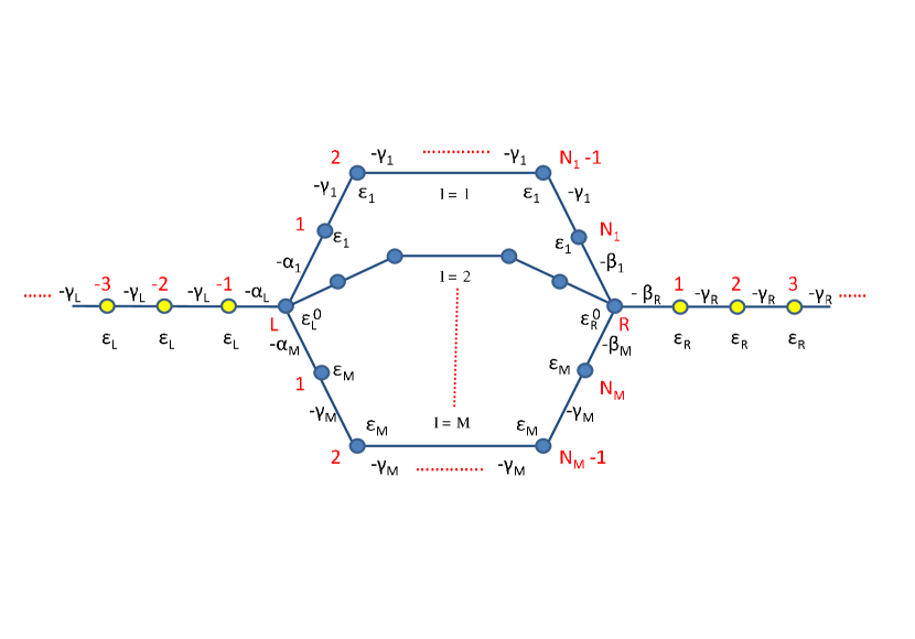
Figure 1: A multi-branch structure with nodal sites $L$ and $R$ on the left and right, connected to external current-carrying leads, by hopping matrix elements $-\alpha_{L}$ on the left and $-\beta_{R}$ on the right and to internals branches {$l$} by hopping matrix elements $-\alpha_{l}$ and $-\beta_{l}$ respectively. The energies of the nodal sites are $\varepsilon_{L}^{0}$ and $\varepsilon_{R}^{0}$. The site energy and hopping matrix element of branch $l$ are $\varepsilon_{l}$ and $-\gamma_{l}$ respectively.

II An analytical formula for electron transport through multi-branch structures

Fig. (1) represents a tight-binding (Hückel-type) model of a multi-branch structure, in which each atom is assigned a single atomic orbital. The structure consists of left and right leads connected to external electron reservoirs (not shown). The atoms of the left lead ($L$) are labelled $j=-1,-2,-3,\dots$. The orbital energy of each atom is denoted $\varepsilon_{L}$ and these are coupled to each other by a nearest-neighbour matrix element $-\gamma_{L}$. Similarly, the atoms of the right lead labelled $j=1,2,3,\dots$, are assigned orbital energies $\varepsilon_{R}$ and these are coupled to each other by a nearest-neighbour matrix element $-\gamma_{R}$. The loop structure comprises $M$ branches, labelled $l=1,2,\dots,M$. Branch $l$ possesses $N_{l}$ atoms, labelled $n_{l}=1,2,\dots,N_{l}$, with atomic-orbital energies $\varepsilon_{l}$, coupled by nearest neighbour matrix elements $-\gamma_{l}$. (Note that hopping matrix elements could be positive or negative and the inclusion of a minus sign is merely convention. For simplicity, we consider the case of a real hamiltonian, since in molecules, orbital effects due to applied magnetic fields are usually negligible.) The left-most atom ($n_{l}=1$) of each branch is connected by a matrix element $-\alpha_{l}$ to a nodal atom (labelled $L$) of orbital energy $\varepsilon^{0}_{L}$. The latter is connected to the right-most atom of the left lead by a matrix element $-\alpha_{L}$. Similarly, the right-most atom ($n_{l}=N_{l}$)of each branch is connected by a matrix element $-\beta_{l}$ to a nodal atom (labelled $R$) of orbital energy $\varepsilon^{0}_{R}$, which in turn is connected to the left-most atom of the right lead by a matrix element $-\beta_{R}$.

In the presence of an incoming plane wave from the left, the solution to the Schrödinger equation, $\hat{H}\psi=E\psi$, in the left lead ($j\leq-1$) is of the form

$$\psi_{j}^{(L)}=e^{ik_{L}j}+r(E)e^{-ik_{L}j}$$ (1)

Similarly, the solution in branch $l$ can be written

$$\psi_{n_{l}}^{(l)}=A_{l}e^{ik_{l}n_{l}}+B_{l}e^{-ik_{l}n_{l}}$$ (2)

and the wavefunction in the right lead ($j\geq 1$) is of the form

$$\psi_{j}^{(R)}=t(E)e^{ik_{R}j}$$ (3)

Finally, the wavefunction on the left and right nodal atoms will be denoted $\chi_{L}$ and $\chi_{R}$ respectively. In the above equations, $E$ is the energy of the incident electron and $r(E)$ and $t(E)$ are transmission and reflection amplitudes. For a given $E$, the dimensionless wavenumbers in the left and right leads, and in branch $l$ are given by $k_{\eta}=\cos^{-1}\left(\frac{\varepsilon_{\eta}-E}{2\gamma_{\eta}}\right)$ where the index $\eta$ is either $L$, $R$ or $l$ respectively. The corresponding group velocities $(a_{\eta}/\hbar)dE/dk$ can be written $(a_{\eta}/\hbar)v_{\eta}$, where $a_{\eta}$ is the atomic spacing in region $\eta$, $v_{\eta}=2\gamma_{\eta}\sin k_{\eta}$. In what follows, we adopt the convention of choosing real values of $k_{\eta}$, such that $v_{\eta}$ is positive and complex values of $k_{\eta}$, such that Im($k_{\eta}$) is positive.

Our initial goal is to obtain an expression for the transmission amplitude $t(E)$, which as shown in the appendix, can be obtained either by matching wavefunctions at the nodal atoms or by using Green’s functions. According to the Landauer formula, the zero-bias electrical conductance is simply $(2e^{2}/h)T(E_{F})$, where $E_{F}$ is the Fermi energy and

$$T(E)=(v_{R}/v_{L})|t(E)|^{2},$$ (4)

which satisfies $T(E)+R(E)=1$, where $R(E)=|r(E)|^{2}$ is the reflection coefficient. In terms of $T(E)$, the current per unit energy carried by the left and right leads is $(2e/h)T(E)$ and since $T(E)\leq 1$, the current per unit energy in the left and right leads cannot exceed $2e/h$. As we shall see below, for $M>1$, this upper bound does not apply to the current per unit energy carried by the internal branches, which we denote $(2e/h)I_{l}$. Indeed for $M>1$, $I_{l}$ can be either positive or negative and is unbounded.

As shown in the appendix, $T(E)$ can be written

$$T(E)=v_{L}\left({\frac{\alpha_{L}}{\gamma_{L}}}\right)^{2}|G_{RL}|^{2}\left({\frac{\beta_{R}}{\gamma_{R}}}\right)^{2}v_{R}$$ (5)

This expression is very general and shows how the various contributions combine to control the current through a single molecule. Equation (5) shows that the transmission coefficient $T(E)$ is a product of several factors; the ”group velocities” $v_{L}$ and $v_{R}$ describe the ability of the left and right leads to carry a current, $\left(\frac{\alpha_{L}}{\gamma_{L}}\right)$ and $\left(\frac{\beta_{R}}{\gamma_{R}}\right)$ describe the ability of the couplings between the nodal atoms and the external leads to transfer electrons and finally $G_{RL}$ describes the ability of a current from a source at node L to be carried to a current sink at node R. In this expression, $G_{RL}$ describes propagation from the nodal site L to at the nodal site R and is sensitive to quantum interference within the multi-branch structure. Since $v_{L}$ and $v_{R}$ have dimensions of energy, whereas $G_{RL}$ has dimensions of energy^-1, the right hand side of equation (5) is dimensionless, as expected.

As shown in the appendix, $G_{RL}$ is given by

$$G_{RL}=\frac{y}{\Delta},$$ (6)

where

$$\Delta=y^{2}-(a_{L}-x_{L})(a_{R}-x_{R}).$$ (7)

In this equation,

$$y=\sum^{M}_{l=1}y_{l},$$ (8)

$$x_{L}=\sum^{M}_{l=1}x^{L}_{l}$$ (9)

and

$$x_{R}=\sum^{M}_{l=1}x^{R}_{l}$$ (10)

where

$$y_{l}=\alpha_{l}\beta_{l}\sin k_{l}/[\gamma_{l}\sin k_{l}(N_{l}+1)]$$ (11)

$$x^{L}_{l}=\alpha_{l}^{2}\sin k_{l}(N_{l})/[\gamma_{l}\sin k_{l}(N_{l}+1)]$$ (12)

and

$$x^{R}_{l}=\beta_{l}^{2}\sin k_{l}(N_{l})/[\gamma_{l}\sin k_{l}(N_{l}+1)]$$ (13)

Finally, the parameters $a_{L}$ and $a_{R}$ are given by

$$a_{L}=(\varepsilon^{0}_{L}-E)-\frac{\alpha_{L}^{2}}{\gamma_{L}}e^{ik_{L}}$$ (14)

and

$$a_{R}=(\varepsilon^{0}_{R}-E)-\frac{\beta_{R}^{2}}{\gamma_{R}}e^{ik_{R}}$$ (15)

Clearly the parameters $a_{L}$ and $a_{R}$ are independent of the details of the internal branches $l$ and are properties of the left and right leads and their respective nodal atoms only. Properties of the branches are contained within the parameters $x_{L}$, $x_{R}$ and $y$ only. From Eq.(6), $T(E)$ will vanish when y=0. This condition for destructive interference does not depend on the parameters describing the leads ($\varepsilon_{L}^{0}$, $\varepsilon_{R}^{0}$, $\gamma_{L}$, $\gamma_{R}$). Nor does it depend on the parameters describing the contacts to the leads ($\alpha_{L}$, $\varepsilon_{L}$,$\alpha_{R}$, $\varepsilon_{R}$). It is a fundamental property of the branches and their couplings to the nodal sites.

As noted in the appendix, equation (5) is extremely general. With a slight modification of the nodal energies $\varepsilon_{L}^{0}$ and $\varepsilon_{R}^{0}$, it can be used to describe the effect of Fano resonances due to dangling bonds at the nodes. Furthermore, with a slight redefinition of $y_{l}$, $x_{l}^{R}$ and $x_{l}^{L}$, it describes electron transmission arising when the branches are replaced by arbitrary elastic scatterers connected by single bonds to the nodal sites.

An alternative form of equation (5) is obtained by writing $\Delta=\Delta_{1}+i\Delta_{2}$, $a_{L}=\tilde{a}_{L}-i\tilde{\Gamma}_{L}$ and $a_{R}=\tilde{a}_{R}-i\tilde{\Gamma}_{R}$, where $\tilde{a}_{L}=\varepsilon^{0}_{L}-E-(\alpha_{L}^{2}/\gamma_{L})\cos k_{L}$ and $\tilde{\Gamma}_{L}=(\alpha_{L}^{2}/\gamma_{L})\sin k_{L}$ and similarly for $\tilde{a}_{R}$ and $\tilde{\Gamma}_{R}$. With this notation,

$$\Delta_{1}=y^{2}-(x_{L}-\tilde{a}_{L})(x_{R}-\tilde{a}_{R})+\tilde{\Gamma}_{L}\tilde{\Gamma}_{R}$$ (16)

and

$$\Delta_{2}=\tilde{\Gamma}_{R}(x_{L}-\tilde{a}_{L})+\tilde{\Gamma}_{L}(x_{R}-\tilde{a}_{R})$$ (17)

and

$$T(E)=\frac{4\tilde{\Gamma}_{L}\tilde{\Gamma}_{R}y^{2}}{\Delta_{1}^{2}+\Delta_{2}^{2}}$$ (18)

Equation (5) describes the transmission coefficient of the combined structure and allows us to evaluate the current per unit energy $(2e/h)T(E)$ due to incident electrons from the left lead with energies $E$. We shall also be interested in the current per unit energy $(2e/h)I_{l}$ carried by branch $l$. As shown in the appendix, this is given by

$$I_{l}=T(E)y_{l}/y,$$ (19)

which clearly satisfies

$$\sum_{l=1}^{M}I_{l}=T(E).$$ (20)

Unlike $T(E)$, which satisfies $0\leq T(E)\leq 1$, $I_{l}$ can have arbitrary sign and arbitrary magnitude.

Before using equation (5) to describe quantum interference within linear and multi-branch molecules, we consider the simplest choice of a single impurity level, weakly coupled to external left and right leads, by matrix elements $\alpha_{1}$ and $\beta_{1}$ respectively, is shown in Fig(2).

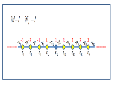
Figure 2: A single impurity in a 1-d chain

This corresponds to the choice $M=1$, $N_{1}=1$, $\gamma_{L}=\alpha_{L}$ $\gamma_{R}=\beta_{R}$, $\varepsilon_{L}=\varepsilon^{0}_{L}$, $\varepsilon_{R}=\varepsilon^{0}_{R}$. In this case equation (5) reduces to the well-known Breit-Wigner formula

$$T(E)={\frac{4\Gamma_{L}\Gamma_{R}}{(E-\varepsilon_{1}+\sigma_{L}+\sigma_{R})^{2}+(\Gamma_{L}+\Gamma_{R})^{2}}}$$ (21)

where $\sigma_{L}=(\alpha_{1}^{2}/\gamma_{L})\cos k_{L}$, $\sigma_{R}=(\beta_{1}^{2}/\gamma_{R})\cos k_{R}$, $\Gamma_{L}=(\alpha_{1}^{2}/\gamma_{L})\sin k_{L}$ and $\Gamma_{R}=(\beta_{1}^{2}/\gamma_{R})\sin k_{R}$.

III Quantum interference in linear molecules or atomic chains.

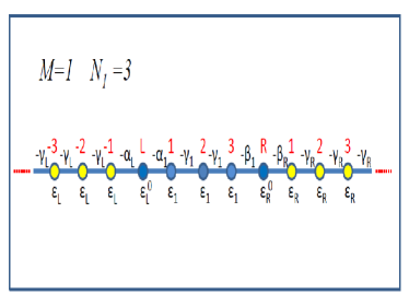
Figure 3: A schematic of the nodal atoms connected by an atomic chain.

The choice $M=1$ $N_{1}>1$ corresponds to the case of external left and right leads, coupled by matrix elements $\alpha_{L}$ and $\beta_{R}$ respectively, to nodal sites $L$ and $R$, which in turn are connected by matrix elements $\alpha_{1}$ and $\beta_{1}$ to an atomic bridge of $N_{1}$ atoms. The case $N_{1}=3$ is shown in Fig(3).

For $M=1$, one obtains

$$y=y_{1}=\frac{\alpha_{1}\beta_{1}}{\gamma_{1}}\frac{\sin k_{1}}{\sin k_{1}(N_{1}+1)}$$ (22)

$$x_{L}=\frac{\alpha_{1}^{2}}{\gamma_{1}}\frac{\sin k_{1}N_{1}}{\sin k_{1}(N_{1}+1)}$$ (23)

$$x_{R}=\frac{\beta_{1}^{2}}{\gamma_{1}}\frac{\sin k_{1}N_{1}}{\sin k_{1}(N_{1}+1)}.$$ (24)

In the case of a metallic or “$\pi$ bridge”, $k_{1}$ will be real. In the case of a ”$\sigma$ bridge”, (which acts as a tunnel barrier), $k_{1}$ will be imaginary and equation (5) (or equivalently equation (18)) describes electron transport via superexchange. Equations (22), (23), (24) highlight a curious feature, which occurs at a special energy $E_{c}$, which corresponds to electrons propagating at the band centre of a $\pi$ bridge and at which $k_{1}=\pi/2$. At this energy, $y$, $x_{L}$ and $x_{R}$ become independent of the length $N_{1}$ of the bridge. On the one hand, if the bridge contains an even number of atoms (ie if $N_{1}$ is even), then $x_{R}=x_{L}=0$, $y=(\alpha_{1}\beta_{1}/\gamma_{1})(-1)^{(N_{1}/2)}$ and

$$T(E_{c})={\frac{4\tilde{\Gamma}_{L}\tilde{\Gamma}_{R}(\alpha_{1}\beta_{1}/\gamma_{1})^{2}}{((\alpha_{1}\beta_{1}/\gamma_{1})^{2}-\tilde{a}_{L}\tilde{a}_{R}+\tilde{\Gamma}_{L}\tilde{\Gamma}_{R})^{2}+(\tilde{a}_{L}\tilde{\Gamma}_{R}+\tilde{a}_{R}\tilde{\Gamma}_{L})^{2}}},$$ (25)

On the other hand, if the bridge contains an odd number of atoms, then $x_{L},x_{R}$ and $y$ diverge and

$$T(E_{c})={\frac{4\tilde{\Gamma}_{L}\tilde{\Gamma}_{R}}{(\alpha_{1}^{2}\tilde{a}_{R}+\beta_{1}^{2}\tilde{a}_{L})^{2}+(\alpha_{1}^{2}\tilde{\Gamma}_{R}+\beta_{1}^{2}\tilde{\Gamma}_{L})^{2}}},$$ (26)

which is independent of the length $N_{1}$ of the bridge. This situation can arise, for example, in the case of oligoynes connected to external electrodes.

These predictions are shown in Fig.(4) for increasing numbers of atoms in the wire, $N_{1}=2,4,6$ and $8$. At the critical energy $E_{c}\approx 0.5{\rm eV}$, all curves intersect. Consequently, for energies $E$ slightly greater than $E_{c}$, $T(E)$ will either increases monotonically as the length of the bridge increases by 2, and for $E$ slightly less than $E_{c}$, $T(E)$ will decrease when the length of the bridge increases. This effect is a clear manifestation of phase-coherent quantum transport.

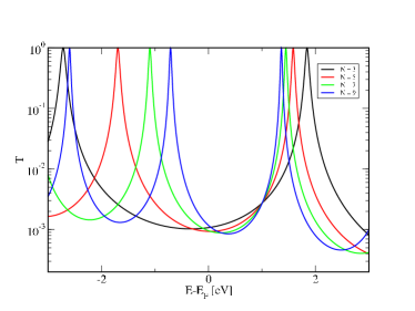
Figure 4: Transmission functions for increasing lengths of molecular wire using the general formula. The system is modelled using the following parameters, in the leads $\varepsilon_{L}=\varepsilon_{R}=0.0$ and $\gamma_{L}=\gamma_{R}=5.0$, for the contacts $\varepsilon_{L}^{0}=\varepsilon_{R}^{0}=-0.4$, in the chain $\varepsilon_{1}=0.5$ and $\gamma_{1}=6.0$ and the coupling between the wire and the electrodes are defined by $\alpha_{L}=\beta_{R}=3.0$. All curves intersect at $E_{c}\approx 0.5{\rm eV}$. Close inspection reveals that $E\approx-0.2{\rm eV}$ the curves approach each other, but do not intersect at a single energy.

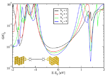
Figure 5: Transmission curves from the SMEAGOL simulations of oligoynes of varying lengths

To demonstrate that this effect is present in atomistic calculations of electron transport, we compare equation (25) with a calculation based on the ab-initio transport code SMEAGOL. This code uses a combination of density functional theory (DFT) DFT and the non-equilibrium Green’s function formalism NEGF to calculate the transport characteristics of atomic scale devices. The DFT Hamiltonian is obtained from the SIESTA code Siesta and is used by SMEAGOL to calculate the electronic density and the transmission. Within the NEGF the system is divided in three parts, the left lead, the right lead and the extended molecule (EM). The EM contains the molecule plus some layers of gold, whose electronic structure is modified due to the presence of the molecule and the surfaces and differs from the bulk electronic structure. The molecular structure consists of an oligoynes capped with phenyl rings and attached to the electrodes by thiolate groups. The SMEAGOL results are shown in Fig.(5), which clearly possesses a critical energy $E_{c}\approx 0.5{\rm eV}$ at which all curves (at least for the longer chains) intersect. The analytic expression assumes that the parameters $\varepsilon_{1}$ and $\gamma$ describing the chains are independent of length. In fact the self-consistent DFT parameters of the shortest chain $(N_{1}=2)$ differ slightly from those of the longer chains and therefore the black curve of figure 5 does not quite pass though the intersection point at $E=E_{c}$.

Clearly the length independence of even and odd chains leads to an even-odd oscillation in the electrical conductance of oligoynes, when $E_{f}$ is close to $E_{c}$. This effect has also been observed in experiments on atomic wires of Au, Pt, and Ir 4 , which exhibit electrical conductance oscillations as a function of the wire length and similar oscillations as a function of bias voltage and electrode separation 5 ; 6 . Several theoretical papers 8 -24 have also addressed these osillations. The above analysis also demonstrates that this effect is present in multi-branch structures, provided the band centres of different branches occur at the same energy.

IV Quantum interference in a two-branch molecule

We now turn to the quantum interference effect transistor (QuIET) discussed in QuIET , which corresponds to the choice $M=2$. To demonstrate that equation (5) (or equivalently (18)) reproduces the key features of a QuIET, we compare it with the results of a detailed simulation using SMEAGOL Smeagol .

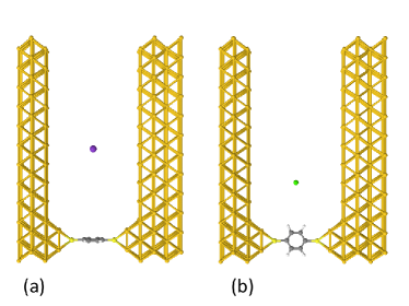
Figure 6: Molecular structure used in the transport simulations with the potassium point charge in configuration C1 (a) and the calcium point charge in configuration C2 (b).

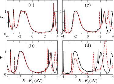
Figure 7: Transmission functions obtained from SMEAGOL simulations with the potassium point charge moving closer to the molecule through (a)-(d). The continuous curve corresponds to C1 and the dashed curve to C2.

The atomic arrangements for the SIESTA/SMEAGOL calculations are shown in Fig. (6). The first arrangement (C1) corresponds to the point charge located along a line perpendicular to the plane of the molecule and which passes through its center. In this configuration the point charge produces a symmetric voltage which affects the two branches to the same extent. The second arrangement (C2) corresponds to the point charge located in the plane of the molecule, closer to one branch of the BDT. In this case the two branches are subject to different electrostatic potentials, which induces quantum interferences in the electron transmission through the molecule. Both configurations were simulated using a point charge of either potassium (K) or calcium (Ca), giving a total of four cases. K and Ca are alkali and alkaline-earth atoms with 1 and 2 valence electrons in the last shell, respectively. Due to their high electropositivity both atoms lose their valence electrons when they are inserted in the unit cell and become ionized with a charge of +e and +2e, respectively. The complete removal of the valence electrons from these atoms can be ensured by reducing the cutoff radii of their orbitals to 3.5 Bohr, which confine the electrons in the atom more closely and therefore increase their energy, making sure they move to lower energy states in the extended molecule. The basis sets used in the simulation were single-zeta (SZ) for the point charge and double-zeta polarized (DZP) for all other elements. The exchange and correlation potential was calculated with the generalized gradient approximation (GGA) and the Perdew-Burke-Ernzerhof parametrization PBE . The gold leads were grown along the (001) direction, and each side of the extended molecule had 3 and 5 layers, respectively, with 36 atoms (12$\times$3 atoms) per layer. The molecule was contacted in a hollow configuration to four additional gold atoms on each side. Since the system was much larger in the $x$ (3 atoms) than in the $y$ direction (12 atoms to leave space for the charge to move), 1 $k$-point was used along $x$ and 4 $k$-points along $y$.

The results are shown in Fig. (7) and Fig. (8), for potassium and calcium, respectively. Each graph contains two curves, corresponding to the cases C1 and C2. In plot (a) the charge is located at a far distance, $\sim 15$ Å from the molecule, and therefore both C1 and C2 produce the same curve. From (b) to (d) the charge is gradually moved towards the molecule (6.29, 5.29 and 4.79 Å away from the center of the ring in (b), (c) and (d), respectively).

We observe that when the charge moves towards the molecule the peaks shift in energy in the negative direction due to the positive potential. However the effect is different depending on where the charge is located relative to the ring. As can be seen, there is a clear difference in both Fig. (7) and Fig. (8) between the continuous and dashed transmission curves in graphs (b)-(d). An extra peak in the dashed transmission curve (C2) appears and the height of the HOMO peak is reduced, whereas the continuous transmission curve (C1) is simply shifted to lower energies without much change in the resonances. Also, through comparison of (a) and (d) we notice a clear narrowing of the HOMO and broadening of the LUMO peak in all cases. We observe a clear reduction of the transmission at the Fermi energy when the charge is located closer to one arm of the molecule (C2). In contrast, for system C1, there is very little change of the transmission about the Fermi energy, because the point charge produces the same phase shifts in the two branches and therefore does not modify interference effects associated with coherent superposition of waves propagating along separate paths.

We also checked the projected density of states (PDOS) on each branch of the BDT to see the specific effect of the charge on the electronic structure in each case. In C1 the PDOS on each branch remains equally distributed and simply shifts to lower energies. However, in C2 there is a clear difference in the PDOS on each branch; the PDOS on the closest branch to the charge is more affected and shifted to lower energies than the PDOS of the opposite branch. This supports the observation of the previously suggested QIE.

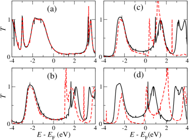
Figure 8: Transmission functions obtained from SMEAGOL simulations with the calcium point charge moving closer to the molecule through (a)-(d). The continuous curve corresponds to C1 and the dashed curve to C2.

To elucidate the underlying physics, we employ Eq. (5) to model electron transmission through a two-branch structure. In the absence any charge, we choose the hopping parameters $\alpha_{L}=\beta_{R}=1.5$, $\gamma_{L}=\gamma_{R}=4.0$ and $\gamma_{1}=\gamma_{2}=1.0$ and the on-site energies $\varepsilon_{L}^{0}=\varepsilon_{R}^{0}=2.0$, $\varepsilon_{1}=0.0,\varepsilon_{2}=0.0$ and $\varepsilon_{L}=\varepsilon_{R}=4.0$. This leads to the transmission curve shown in Fig. (9) (a), which is very close to the ab-initio result. In configuration C1, where a charge affects both branches equally, the presence of a charge is modelled by shifting the on-site energies $\varepsilon_{L}$, $\varepsilon_{1}$, $\varepsilon_{2}$ and $\varepsilon_{R}$, upwards or downwards by the same amount, which depends on the sign and strength of the charge. The outcome produced by a positive charge is represented by the continuous transmission curves in Fig. (9). The charge moves closer to the ring from (b) to (d) and the parameters are chosen as follows (b) $\varepsilon_{L}^{0}=\varepsilon_{R}^{0}=1.4$, $\varepsilon_{1}=\varepsilon_{2}=-0.8$, (c) $\varepsilon_{L}^{0}=\varepsilon_{R}^{0}=1.2$, $\varepsilon_{1}=\varepsilon_{2}=-1.8$, (d) $\varepsilon_{L}^{0}=\varepsilon_{R}^{0}=1.0$, $\varepsilon_{1}=\varepsilon_{2}=-2.0$. In each of these plots, $\varepsilon_{L}=\varepsilon_{R}$ remain unchanged throughout. As in the ab-initio simulations we see that the entire transmission curve is shifted to lower energies and quantum interference effects are negligible. Interestingly, as a consequence of this shift and the corresponding change in the electronic structure, the width of the variability in the local density of states at the contact, the width of the HOMO decreases and the width of the LUMO increases, in agreement with the ab-initio results.

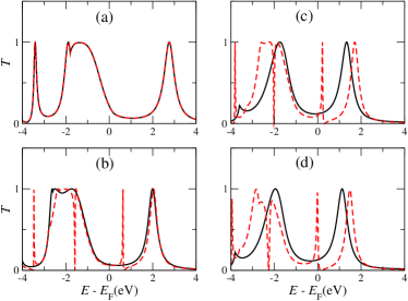
Figure 9: Transmission curves for the tight binding model. The continuous line corresponds to the case where the charge is located along a line perpendicular to the ring and which passes through its center. The dashed line corresponds to the case where the charge is closer to one arm. Panel (a) shows the transmission curves when the charge is away from the molecule. From panel (b) to (d) the onsite energy parameters are changed to simulate the charge moving towards the molecule.

To produce quantum interference, we now examine the effect of a scanning point charge placed in configuration C2; i.e. closer to one branch of the ring. To model this effect using Eq. (18), the parameters are now adjusted asymmetrically; i.e. they are changed less in the branch which is far away from the charge and more in the branch which is closer. The adjustment also includes changing the contact points $\varepsilon_{L}^{0}$ and $\varepsilon_{R}^{0}$ as these will feel a smaller effect from the charge than the nearer branch. The adjusted parameters are chosen as follows (b) $\varepsilon_{L}^{0}=\varepsilon_{R}^{0}=1.35$, $\varepsilon_{1}=-1.0$, $\varepsilon_{2}=-0.5$ (c) $\varepsilon_{L}^{0}=\varepsilon_{R}^{0}=1.1$, $\varepsilon_{1}=-1.5$, $\varepsilon_{2}=-0.8$ (d) $\varepsilon_{L}^{0}=\varepsilon_{R}^{0}=1.0$, $\varepsilon_{1}=-1.8$ and $\varepsilon_{2}=-0.9$. As before, $\varepsilon_{L}=\varepsilon_{R}$ and are unchanged. The transmission corresponding to these parameters is shown Fig.(9) (dashed curves), where the point charge is brought successively closer to the molecule from (b) to (d). We see again from (a) through to (d) that the peaks have all shifted to lower energies, but the HOMO dramatically changes and reduces its height. Also, an additional peak appears due to the point charge effect on the electronic structure on only one arm of the molecule, which causes interferences in the transmission through the system. This again agrees with the SMEAGOL simulations and suggests this analytical model captures the qualitative features of transmission in ring-like molecules.

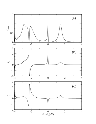
Figure 10: (a) Total current through the molecule, (b), and the current through branch 1, (c), and branch 2 of the molecule. Parameters used are exactly as the dashed red line in Fig 9(d), namely $\varepsilon_{R}=\varepsilon_{L}=4.0$, $\varepsilon_{L}^{0}=\varepsilon_{R}^{0}=1.0$, $\varepsilon_{1}=-1.8$, $\varepsilon_{2}=-0.9$ $\gamma_{L}=\gamma_{R}=4.0$, $\gamma_{1}=\gamma_{2}=1.0$, $\alpha_{L}=\beta_{R}=1.5$.

Having established that the analytical model captures the essential features of the ab-initio simulations, we now show how this model can be employed to examine the internal currents within different branches of the molecule, which are obtained by evaluating equation (19). When the ion located close to branch $1$, the lower graphs of Fig. (10) show the internal currents $I_{1}$ and $I_{2}$ through the individual branches, whereas the upper graph shows the total current $I_{\rm TOT}=I_{1}+I_{2}=T(E)$. Figs. (10) (b) and (c) clearly demonstrate that the current in a single branch can greatly exceed the total current through the molecule when a counter current of opposite sign occurs in the other branch of the molecule and can clearly exceed the upper bound of $I_{\rm TOT}=1$. The appearance of such unbounded counter currents is yet another manifestation of quantum interference within single molecules. loop .

V Summary

In conclusion, we have presented ab initio simulations and an analytical formula, which highlights a range of interference effects in single and multi-branch structures. The analytical solution is rather versatile and has the advantage that it can be evaluated on a pocket calculator. It provides insight into length-independent electrical conductances for even and odd oligoyne chains, when the Fermi energy coincides with the band centre of the oligoyne bridge and allows us to predict that this behaviour is also present in multi-branch structures, provided the branches share a common band centre. As demonstrated in the manuscript the energy $E_{c}$ at which this odd-even effect occurs corresponds to $k1=\pi/2$. This condition is very general and is independent of the nature of the orbitals. For the particular case of oligoynes, this is a consequence of $\pi$ coherent transport, but for other systems, such a metallic wires, this would not be the case. The case $M=1$ demonstrates that quantum interference does not require the presence of physically different paths, because even in this case, interference due to scattering from nodal impurity sites and connections to external leads arises from the amplitudes $a_{L}$ and $a_{R}$ in equations (14) and (15). Both the magnitudes and phases of these amplitudes appear on the right hand side of equation (7) and therefore even for a single-branch system, they contribute to interference.

Ab initio simulations based on density functional theory, demonstrate the presence of quantum interference in BDT, due to electrostatic interactions associated with a scanning point charge positioned close to the molecule. We have shown that a scanning charge located within the plane of a BDT molecule produces a sizeable quantum interference, whereas a charge approaching the molecule along a line perpendicular to the plane produces a much smaller effect, in agreement with the analytical formula. In spite of the consistency between the TB result and the ab initio result for the BDT system, there are of course quantitative differences between them. In part this arises because the tight-binding model includes only a single (”$\pi$”) orbital per atom, whereas the ab initio description includes both $\pi$ transport and $\sigma$ tunneling. In addition, the tight-binding model includes only a single scattering channel in each lead, whereas the ab initio model contains multiple channels.

Using the analytical model, we have also investigated the internal currents within a two-branch molecule and demonstrated that large currents and counter currents can occur, which exceed an upper bound for the total current through the molecule.

VI Appendix I: Derivation of equation 5 for transmission though the multi-branch structure of figure (1).

We derive the equation for $T(E)$ by matching wave functions at the nodes of a multi-branch structures and later make a comparison with results obtained from a corresponding Green’s function analysis. The starting point is the tight binding Schrödinger equation, which can be written

$$\varepsilon_{\mu}\psi_{\mu}-\sum_{\nu}\gamma_{\nu,\mu}\psi_{\nu}=E\psi_{\mu},$$ (27)

where the summation is over all nearest neighbours $\nu$ of site $\mu$. Choosing $\mu$ to label the site just to the left of the nodal site $L$ (whose wave function is denoted $\chi_{L}$) yields $\varepsilon_{L}\psi_{-1}^{(L)}-\gamma_{L}\psi_{-2}^{(L)}-\alpha_{L}\chi_{L}=E\psi_{-1}^{(L)}$, where $\gamma_{L}=\gamma{-1,-2}$ and $\alpha_{L}=\gamma_{L,-1}$. From this expression, and noting that the Schrödinger equation in the left lead takes the form of a recurrence relation recur , the wave function at the node $L$ is given by

$$\chi_{L}=\frac{\gamma_{L}(1+r)}{\alpha_{L}}$$ (28)

Similarly, choosing $\mu$ to label the site just to the right of the nodal site $R$ (whose wave function is denoted $\chi_{R}$) yields

$$\chi_{R}=\frac{\gamma_{R}t}{\beta_{R}}.$$ (29)

Choosing $\mu$ to label the first site ($1_{l}$) of chain $l$ yields for all $l$,

$$\chi_{L}=(\gamma_{l}/\alpha_{l})(A_{l}+B_{l})$$ (30)

and choosing $\mu$ to label the last site ($N_{l}$ of chain $l$ yields for all $l$,

$$\chi_{R}=(\gamma_{l}/\beta_{l})(A_{l}e^{ik_{l}(N_{l}+1)}+B_{l}e^{-ik_{l}(N_{l}+1)})$$ (31)

Finally choosing $\mu$ to label the nodal sites $L$ and $R$ yields

$$\varepsilon^{0}_{L}\chi_{L}-\sum_{l=1}^{M}\alpha_{l}\psi^{(l)}_{1}-\alpha_{L}(e^{-ik_{L}}+r(E)e^{ik_{L}})=E\chi_{L}$$ (32)

and

$$\varepsilon^{0}_{R}\chi_{R}-\sum_{l=1}^{M}\beta_{l}\psi^{(l)}_{N_{l}}-\beta_{R}t(E)e^{ik_{R}}=E\chi_{R}$$ (33)

Equations (28) with (32) and(29) with (33) combine to yield

$$\chi_{L}=\frac{\gamma_{L}}{\alpha_{L}}(1+r)=\frac{\sum_{l=1}^{M}\alpha_{l}\psi_{1}^{(l)}-2\alpha_{L}i\sin(k_{L})}{a_{L}}$$ (34)

and

$$\chi_{R}=\frac{\gamma_{R}}{\beta_{R}}t=\frac{\sum_{l=1}^{M}\beta_{l}\psi_{N_{l}}^{(l)}}{a_{R}}$$ (35)

where $a_{L}$ and $a_{R}$ are given by equations (14) and (15).

From the form of the wave functions in the branches, given by equation (2), these can be written

$$\left(\begin{array}[]{c}\chi_{L}\\ \chi_{R}\end{array}\right) = \frac{1}{a_{L}}\left(\begin{array}[]{c}-2i\alpha_{L}\sin(k_{L})\\ 0\end{array}\right)$$ (45)

$$+\sum_{l=1}^{M}\left(\begin{array}[]{cc}\frac{\alpha_{l}e^{ik_{l}}}{a_{L}}&\frac{\alpha_{l}e^{-ik_{l}}}{a_{L}}\\ \frac{\beta_{l}e^{ik_{l}N_{l}}}{a_{R}}&\frac{\beta_{l}e^{-ik_{l}N_{l}}}{a_{R}}\end{array}\right)\left(\begin{array}[]{c}A_{l}\\ B_{l}\end{array}\right)$$

Since equations (30) and (31) yield

$$\left(\begin{array}[]{c}A_{l}\\ B_{l}\end{array}\right)=\frac{1}{-2i\gamma_{l}\sin k_{l}(N_{l}+1)}\left(\begin{array}[]{cc}\alpha_{l}e^{-ik_{l}(N_{l}+1)}&-\beta_{l}\\ -\alpha_{l}e^{ik_{l}(N_{l}+1)}&\beta_{l}\end{array}\right)\left(\begin{array}[]{c}\chi_{L}\\ \chi_{R}\end{array}\right)$$ (46)

$A_{l}$ and $B_{l}$ can be eliminated from equation (45) to yield

$$\\ \left(\begin{array}[]{c}\chi_{L}\\ \chi_{R}\end{array}\right)=G\left(\begin{array}[]{c}2i\alpha_{L}\sin(k_{L})\\ 0\end{array}\right)=\left(\begin{array}[]{c}G_{LL}\\ G_{RL}\end{array}\right)2i\alpha_{L}\sin(k_{L})$$ (47)

In this expression, the matrix $G$ has the form

$$G=\left(\begin{array}[]{cc}G_{LL}&G_{LR}\\ G_{RL}&G_{RR}\end{array}\right)$$ (50)

and is given by

$$G^{-1}=\left(\begin{array}[]{cc}{-a_{L}}&0\\ 0&{-a_{R}}\end{array}\right)+\left(\begin{array}[]{cc}{x_{L}}&y\\ y&{x_{R}}\end{array}\right)$$ (55)

where $x_{L}$, $x_{R}$ and $y$ are given by equations (8), (9) and (10). From this expression, one obtains $\chi_{R}$ and hence the transmission amplitude $t$, via equation (29).

The physical meaning of the various contributions to the above expressions can be understood by carrying out a parallel analysis based on Green’s functions andres ; brand , which reveals that equation (55) is simply Dyson’s equation for the Green’s function matrix elements involving the nodal sites $L$ and $R$. Comparison with Refs. andres ; brand also demonstrates that $v_{L}(\alpha_{L}/\gamma_{L})^{2}$ and $v_{R}(\alpha_{R}/\gamma_{R})^{2}$ in Eq,(5) are imaginary parts of the self-energies of the left- and right-hand electrodes, respectively.

This is demonstrated by noting that the Green’s function for a finite linear chain of $N_{l}$ sites, with nearest-neighbour hopping elements $-\gamma_{l}$ and diagonal elements $\varepsilon_{l}$ is

$$g_{l}(n_{l},n^{\prime}_{l})=\begin{array}[]{cc}A_{l}\sin k_{l}n_{l}\sin k_{l}[n^{\prime}_{l}-(N_{l}+1)]&({\rm for}\,n_{l}\leq n^{\prime}_{l})\\ A_{l}\sin k_{l}n^{\prime}_{l}\sin k_{l}([n_{l}-(N_{l}+1)]&({\rm for}\,n^{\prime}_{l}\leq n_{l})\\ \end{array}$$ (57)

where $A_{l}=1/[\gamma_{l}\sin k_{l}\sin k_{l}(N_{l}+1)]$. An alternative form of this expression is $g_{l}(n_{l},n^{\prime}_{l})=(A_{l}/2)(\cos k_{l}[N_{l}+1-|n_{l}-n^{\prime}_{l}|]-\cos k_{l}[N_{l}+1-n_{l}-n^{\prime}_{l}])$

The quantity $g_{l}(n_{l},n^{\prime}_{l})$ is the Greens function matrix element connecting atom $n_{l}$ to atom $n^{\prime}_{l}$ of the decoupled branch $l$, which would arise when $\alpha_{l}=\beta_{l}=0$. The off-diagonal matrix element describing propagation from one end of such a branch to the other is

$$g_{l}(1_{l},N_{l})=-\sin k_{l}/{\gamma_{l}\sin k_{l}(N_{l}+1)}$$ (58)

whereas the diagonal matrix element evaluated on an end atom is

$$g_{l}(1_{l},1_{l})=g_{l}(N_{l},N_{l})=-\sin k_{l}N_{l}/{\gamma_{l}\sin k_{l}(N_{l}+1)}$$ (59)

As expected, these quantities diverge when $\sin k_{l}(N_{l}+1)=0$, which corresponds to the eigenenergies of an isolated branch. In terms of these Greens functions,

$$y_{l}=-\alpha_{l}\beta_{l}g_{l}(1,N_{l})$$ (60)

$$x^{L}_{l}=-\alpha_{l}^{2}g_{l}(1_{l},1_{l})$$ (61)

and

$$x^{R}_{l}=-\beta_{l}^{2}g_{l}(N_{l},N_{l})$$ (62)

Within a Green’s function approach, one defines the nodal self energy matrix $\sigma$ to be

$$\sigma=\sum_{l=1}^{M}\sigma_{l}$$ (63)

where $\sigma_{1}$ is the contribution to the self-energy from branch $l$, given by

$$\sigma_{l}=\left(\begin{array}[]{cc}{-\alpha_{l}}&0\\ 0&{-\beta_{l}}\end{array}\right)g_{l}\left(\begin{array}[]{cc}{-\alpha_{l}}&0\\ 0&{-\beta_{l}}\end{array}\right)$$ (68)

In this expression $g_{l}$ is the Greens function connected the end atoms of an isolated branch:

$$g_{l}=\left(\begin{array}[]{cc}g_{l}(1_{l},1_{l})&g_{l}(1_{l},N_{l})\\ g_{l}(N_{l},1_{l})&g_{l}(N_{l},N_{l})\end{array}\right)$$ (70)

This demonstrates that

$$\left(\begin{array}[]{cc}x_{L}&y\\ y&x_{R}\end{array}\right)=-\sigma$$ (71)

and therefore equation (55) takes the form of Dyson’s equation:

$$G^{-1}=\left(\begin{array}[]{cc}{g^{-1}_{L}}&0\\ 0&{g^{-1}_{R}}\end{array}\right)-\sigma$$ (72)

where $g_{L}=-a^{-1}_{L}$ and $g_{R}=-a_{R}^{-1}$ are diagonal elements of the Greens function of the decoupled semi-infinite chains (obtained by setting all $\alpha_{l}=\beta_{l}=0$), evaluated on the left (L) and right (R) nodal sites respectively. This also demonstrates that the form of equation(5) and in particular $G_{RL}$ does not change even when the branches $l$ are replaced by arbitrary elastic scattering regions, connected to nodal sites by bonds $\alpha_{l}$ and $\beta_{l}$, provided $g_{l}$ is replaced by the Green’s function of the $l$th scattering region. With this redefinition of $y_{l}$, the condition for destructive interference ($y=0$) remains unchanged. For example, if instead of a linear chain of $n_{l}$ sites, branch $l$ is replaced by a loop of $n_{l}$ sites, , then equation (57) is replaced by the Greens function of a linear chain of $n_{l}$ sites with periodic boundary conditions, namely $g_{l}(n_{l},n^{\prime}_{l})=(\cos k_{l}[N_{l}/2-|n_{l}-n^{\prime}_{l}|])/(2\gamma\sin k_{l}\sin[k_{l}N_{l}/2])$ and equation (70) is replaced by

$$g_{l}=\left(\begin{array}[]{cc}g_{l}(n_{l},n_{l})&g_{l}(n_{l},m_{l})\\ g_{l}(m_{l},n_{l})&g_{l}(m_{l},m_{l})\end{array}\right),$$ (73)

where $n_{l}$ and $m_{l}$ label the sites of the loop connected to the nodal sites $L$ and $R$ respectively. Taking this to an extreme, any of the branches $l$ could even be replaced by a multi-branch scatterer, simply by replacing $g_{l}$ by the Greens function of an isolated multi-branch system, obtained from $G$ by setting $\alpha_{L}=\beta_{R}=0$.

The above analysis, which focusses on the wave-like nature of Greens functions is rather different in spirit from alternative approaches which emphasise the algebraic nature of Greens functions, which for finite structures, take the form of ratios of polynomials, whose denominator is proportional to the secular equation ratner . To make contact with this approach, we note that equation (72) yields

$$G=\frac{-1}{\Delta}\left(\begin{array}[]{cc}x-a_{R}&-y\\ -y&x-a_{L}\end{array}\right)$$ (74)

where $\Delta=\Delta_{1}+i\Delta_{2}$, and therefore the equation $\Delta_{1}=0$ is the secular equation for the isolated multi-branch structure, which arises when $\alpha_{L}=\beta_{R}=0$. More generally, from equations (16) and (17), the equation $\Delta_{1}=\tilde{\Gamma}_{L}\tilde{\Gamma}_{R}$ is the secular equation for the same isolated system, but with the site energies of the nodal atoms shifted by the real part of their respective self energies.

Finally the current per unit energy in branch $l$, carried by electrons of energy $E$ injected from the left lead is $(2e/h)I_{l}$, where

$$I_{l}=\frac{v_{l}}{v_{L}}(|A_{l}|^{2}-|B_{l}|^{2})$$ (75)

Expressions for $A_{l}$ and $B_{l}$ are obtained from equation (46), which combine to yield equation(19) of the main text.

The above comparison between the wave-function-matching and Green’s function underpins a deep understanding of equation (47), because if $\mu\leq-1$ labels a site in the left lead and $\nu\geq\mu$ labels a site inside the scattering region or in the right lead, then the wave function $\psi_{\nu}$ is related to $G_{\nu,\mu}$ by the expression

$$\psi_{\nu}=2i\gamma_{L}\sin k_{L}e^{ik_{L}\mu}G_{\nu,\mu}$$ (76)

Furthermore, starting from the limit $\alpha_{L}=0$ and then including the effect of $\alpha_{L}$ via Dyson’s equation yields $G_{LL}=(\gamma_{L}/\alpha_{L})e^{-ik_{L}}G_{L,-1}$ and $G_{RL}=(\gamma_{L}/\alpha_{L})e^{-ik_{L}}G_{R,-1}$. Hence equation (47) can be written in the intuitive form

$$\left(\begin{array}[]{c}\chi_{L}\\ \chi_{R}\end{array}\right)=\left(\begin{array}[]{c}G_{L,-1}\\ G_{R,-1}\end{array}\right)e^{-ik_{L}}2i\gamma_{L}\sin(k_{L}),$$ (77)

which is simply an example of equation (76), with $\mu=-1$ and $\nu=L$ or $R$.

As mentioned in the main text, equation(5) is extremely versatile. For example, the case of $M=1$ $N_{1}>1$, can be used to describe a donor-bridge-acceptor molecules. In this case, to obtain a simple description of rectification, all parameters should be assigned and appropriate dependence on the applied voltage $V$. The simplest model is obtained by setting $\epsilon_{L}(V)=\epsilon_{L}(0)+eV/2$, $\epsilon^{0}_{L}(V)=\epsilon^{0}_{L}(0)+eV/2$, $\epsilon_{R}(V)=\epsilon_{R}(0)-eV/2$ $\epsilon^{0}_{R}(V)=\epsilon^{0}_{R}(0)-eV/2$, and then computing the current via the expression $I=\int^{E_{F}+eV/2}_{E_{F}-eV/2}T(E)dE$.

To further demonstrate the versatility of equation(19), we end this appendix by noting that it readily describes the effect of Fano resonances on transport and the effect of coupling to a molecule at different points along its length. To illustrate this, consider a structure in which dangling branches, labelled $l=0$ and $l=M+1$, are attached by couplings $\alpha_{0}$ and $\beta_{M+1}$ to the nodal sites on the left and right respectively, as shown in figure (11).

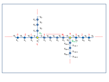
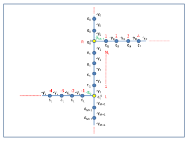
Figure 11: A diagram to show the case of a molecule with dangling branches. The top and bottom panels show two equivalent representations of the same system.

In this case, equations (5) and (18) are unchanged, except that $\varepsilon_{R}^{0}$ and $\varepsilon_{L}^{0}$ are renormalised by the self energies of the dangling branches, and replaced by

$$\tilde{\varepsilon}_{R}^{0}=\varepsilon_{R}^{0}+\beta_{M+1}^{2}g_{M+1}$$ (78)

and

$$\tilde{\varepsilon}_{L}^{0}=\varepsilon_{L}^{0}+\alpha_{0}^{2}g_{0},$$ (79)

where

$$g_{0}=-\frac{\sin k_{0}N_{0}}{\gamma_{0}\sin k_{0}(N_{0}+1)}$$ (80)

and

$$g_{M+1}=-\frac{\sin k_{M+1}N_{M+1}}{\gamma_{M+1}\sin k_{M+1}(N_{M+1}+1)}$$ (81)

Clearly an anti-resonance occurs when the energy $E$ coincides with an eigen-energy of either of the two branches, because at these energies, one of the Green’s functions $g_{0}$ or $g_{M+1}$ diverges and therefore one of the renormalised nodal site energies $\tilde{\varepsilon}_{R}^{0}$ or $\tilde{\varepsilon}_{L}^{0}$ diverges. This is equivalent to introducing an infinite potential at one of the nodes and therefore at these energies, $T(E)$ vanishes. This behaviour arises from the interaction between bound states in the dangling branches and the continuum of states associated with the external leads and is typical of a Fano resonance.

By redrawing Figure figure (11a) as shown in figure (11b), one can see that the above equation describes a linear molecule contacted at atoms within the length of the molecule, rather than simply at the end atoms. As an example, consider the case when $M=1$, $\varepsilon_{1}=\varepsilon_{0}=\varepsilon_{2}=\varepsilon_{L}=\varepsilon_{R}$, $\gamma_{1}=\gamma_{0}=\gamma_{2}=\alpha_{0}=\beta_{2}=\alpha_{1}=\beta_{1}$. The system then comprise a linear chain of length $L=N_{0}+N_{1}+N_{2}+2$ sites, connect to external leads by nodal sites located at positions $N_{0}+1$ and $N_{1}+N_{0}+2$ along the chain. By varying $N_{0}$ and $N_{1}$ but with fixed $L$, the expression for $T(E)$ then describes quantum interference effects which arise when external leads are connected to a fixed length molecule, at different locations along its length.

References

- (1) G. Cuniberti, G. Fagas, and K. Richter, Introducing Molecular Electronics (Springer-Verlag, Berlin, 2005).
- (2) N. J. Tao, Nature Nanotech. 1 , 173-181 (2006).
- (3) A. Nitzan, M. A. Ratner, Science , 300 , 1384-1389 (2003).
- (4) G.J. Ashwell, B. Urasinska, C.S. Wang, et al., Chem. Comm. 45 4706 (2006)
- (5) S. H. Ke, W. Yang and H. U. Baranger, Nano Lett. 8, 3257 (2008).
- (6) R. Stadler, Phys. Rev. 80, 125401 (2009).
- (7) C. A. Stafford, D. M. Cardamone, and S. Mazumdar, Nanotechnology 18, 424014 (2007).
- (8) R. Stadler, M. Forshaw, and C. Joachim, Nanotechnology 14 138 (2003).
- (9) C. Joachim, J. K. Gimzewski, and A. Aviram, Nature 408, 541 (2000).
- (10) R. Baer and D. Neuhauser J. Am. Chem. Soc. 124, 4200-4201, 2002
- (11) A. R. Rocha, V. M. García-Suárez, S. W. Bailey, C. J. Lambert, J. Ferrer, and S. Sanvito, Nature Materials 4, 335 (2005).
- (12) P. Hohenberg and W. Kohn, Phys. Rev. 136, B864 (1964); W. Kohn and L. J. Sham, Phys. Rev. 140, A1133 (1965).
- (13) L. V. Keldysh, Sov. Phys. JETP 20, 1018 (1965); C. Caroli, R. Combescot, P. Nozieres, and D. Saint-James, J. Phys. C: Solid State Phys. 5, 21 (1972).
- (14) J. M. Soler, E. Artacho, J. D. Gale, A. García, J. Junquera, P. Ordejón and D. Sánchez-Portal, J.Phys.: Condens. Matter 14, 2745 (2002).
- (15) J. P. Perdew, K. Burke, and M. Ernzerhof, Phys. Rev. Lett. 77, 3865 (1996).
- (16) S. Nakanishi and M. Tsukada, Jpn. J. Appl. Phys. Vol. 37 (1998)
- (17) R. H. M. Smit, C. Untiedt, G. Rubio-Bollinger, R. C. Segers, and J. M. van Ruitenbeek, Phys. Rev. Lett. 91 , 076805 (2003).
- (18) B. Ludoph, M. H. Devoret, D. Esteve, C. Urbina, and J. M. van Ruitenbeek, Phys. Rev. Lett. 82, 1530 (1999).
- (19) A. Halbritter, Sz. Csonka, G. Mihály, O. I. Shklyarevskii, S. Speller, and H. van Kempen, Phys. Rev. B 69, 121411 (2004).
- (20) J. Ferrer, A. Martín-Rodero, and F. Flores, Phys. Rev. B 38, R10113 (1988).
- (21) N. D. Lang and Ph. Avouris, Phys. Rev. Lett. 81, 3515 (1998).
- (22) E. G. Emberly and G. Kirczenow, Phys. Rev. B 60, 6028 (1999).
- (23) N. D. Lang and Ph. Avouris, Phys. Rev. Lett. 84, 358 (2000).
- (24) N. Kobayashi, M. Brandbyge, and M. Tsukada, Phys. Rev. B 62, 8430 (2000).
- (25) H.-S. Sim, H.-W. Lee, and K. J. Chang, Phys. Rev. Lett. 87, 096803 (2001).
- (26) R. Gutiérrez, F. Grossmann, and R. Schmidt, Acta Phys. Pol. B 32, 443 (2001).
- (27) H.-W. Lee and C.-S. Kim, Phys. Rev. B 63, 075306 (2001).
- (28) Z. Y. Zeng and F. Claro, Phys. Rev. B 65, 193405 (2002).
- (29) P. Havu, T. Torsti, M. J. Puska, and R. M. Nieminen, Phys. Rev. B 66, 075401 (2002).
- (30) S. Tsukamoto and K. Hirose, Phys. Rev. B 66, 161402 (2002).
- (31) K. S. Thygesen and K. W. Jacobsen, Phys. Rev. Lett. 91, 146801 (2003).
- (32) K. Hirose, N. Kobayashi, and M. Tsukada, Phys. Rev. B 69, 24 5412 (2004).
- (33) Y. J. Lee, M. Brandbyge, M. J. Puska, J. Taylor, K. Stokbro, and R. M. Nieminen, Phys. Rev. B 69, 125409 (2004).
- (34) P. Major,1 V. M. Garcia-Suarez, S. Sirichantaropass, J. Cserti,3 C. J. Lambert, J. Ferrer and G. Tichy, Phys. Rev. B 73, 045421 (2006)
- (35) C. J. Lambert, J. Phys. C-Sol. State, 17 2401 (1984)
- (36) N.R. Claughton, M. Leadbeater and C.J. Lambert, J. Phys. Condens. Matter, 7 8757 (1995)
- (37) M. Brandbyge et al, Phys. Rev.B 65, 165401 (2002)
- (38) T. Hansen, G.C. Solomon, D.Q. Andrews and M.A. Ratner, J. Chem. Phys. 131 194704 (2009)