Nonlinear terahertz emission in semiconductor microcavities

Abstract

We consider the nonlinear terahertz emission by the system of cavity polaritons in the regime of polariton lasing. To account for the quantum nature of terahertz- polariton coupling we use Lindblad master equation approach and demonstrate that quantum microcavities reveal rich variety of the nonlinear phenomena in terahertz range, including bistability, short THz pulse generation and THz switching.

Introduction. THz band remains the last region of electromagnetic spectrum which does not have wide application in modern technology due to lack of solid state source of THz radiation which is compact, reliable and scalable [Davies, ]. Fundamental objection preventing realization of such source is small rate of spontaneous emission of the THz photons. According to Fermi Golden rule this rate is about tens of inverse milliseconds, while lifetime of the photoexcited carrier typically lies in picosecond range due to the efficient interaction with phonons Duc ; Doan . Spontaneous emission rate can be increased by application of Purcell effect when emitter of THz is placed in cavity for THz mode Todorov1 ; Chassagneux1 , but even in this case cryogenic temperatures are required to provide quantum efficiency of the order about one percent for typical quantum cascade structure.

Recently it was proposed that the rate of spontaneous emission for THz photons can be additionally increased by bosonic stimulation if radiative transition occurs into a condensate state Kavokin1 . One example is a transition between upper and lower polariton branches in semiconductor microcavity in the regime polariton lasing. Unfortunately, the radiative transition accompanied by emission of THz photon between upper and lower polariton modes is forbidden, since these states have the same parity. Nevertheless, such transition becomes possible if upper polariton state is mixed with exciton state of different parity. Amplification of spontaneous emission by Purcell effect together with bosonic stimulation increase the rate of spontaneous emission by several orders of magnitude, making it comparable with the rate of scattering with acoustic phonon. Consequently, effective emission of THz radiation can occur Kavokin1 .

It is well known that strong polariton-polariton interactions in microcavities make it possible to observe pronounced nonlinear effects for the intensities of the pump orders of magnitude smaller than in other nonlinear optical systems. Among them are polariton superfluidity Amo , bistability and multistability Baas ; Gippius , soliton formation Egorov and others. One can expect that polariton-polariton interactions will as well strongly affect the process of THz emission. The quasiclassical approach based on Boltzmann equations, used in Ref.Kavokin1, cannot provide a correct account of a coherent interaction of THz photons and polaritons, and can not be used for satisfactory description of nonlinearities in the considered system. The development of more exact quantum formalism is thus needed. This paper is aimed at building such a formalism, which accounts for the following physical processes: coherent polariton-THz photon interaction, polariton- polariton interaction leading to the blueshift of the polariton modes and coupling of the polaritons with acoustic phonons. The development of such description is timely in light of intensive studies of ultrastrong light-matter coupling [Todorov2, ,Gunter, ], single cycle THz generation Junginger ; Todorov3 , intersubband cavity polariton physics Todorov3 ; Ciuti and control of the phase of THz radiation in both inorganic and organic structures Oustinov ; Swoboda .

Formalism. We consider a model system consisting of a lower polariton state with the energy $\epsilon_{L}$, upper hybrid state with the energy $\epsilon_{U}$, THz cavity mode with the energy $\epsilon_{T}$ and incoherent polariton reservoir coupled with upper and lower polariton states via phonon-assisted process (see Fig.1).

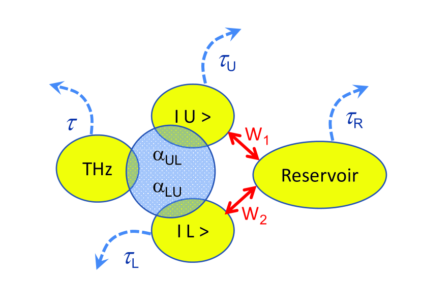
Figure 1: The scheme of transitions in THz emitting cavity. The upper polariton is mixed with dark exciton state due to the application of the gate voltage $V_{g}$. The radiative transition between the upper hybrid state $|U\rangle$ and lower polariton state $|L\rangle$ thus becomes possible. Upper hybrid and lower polariton states are also coupled with an incoherent reservoir of the polaritons via phonon-assisted process.

The Hamiltonial of the system written in terms of the operators of secondary quantization for upper polaritons ($a_{U},a_{U}^{+}$), lower polaritons ($a_{L},a_{L}^{+}$), TH photons ($c,c^{+}$), reservoir states ($a_{R\textbf{k}},a^{+}_{R\textbf{k}}$) and acoustic phonons $b_{\textbf{k}},b^{+}_{\textbf{k}}$ can be represented as a sum of four terms:

$$H=H_{0}+H_{pol-pol}+H_{T}+H_{R}$$ (1)

The first term

$$H_{0}=\epsilon_{L}a^{+}_{L}a_{L}+\epsilon_{U}a^{+}_{U}a_{U}+\epsilon_{T}c^{+}c+\sum_{k}\epsilon_{\textbf{k}}a^{+}_{R\textbf{k}}a_{R\textbf{k}}$$ (2)

corresponds to the energy of uncoupled upper and lower polaritonic states, THz mode and polariton reservoir.

The second term

$$H_{pol-pol}=U_{LL}a^{+}_{L}a^{+}_{L}a_{L}a_{L}+U_{UU}a^{+}_{U}a^{+}_{U}a_{U}a_{U}+$$ (3)

$$+2U_{UL}a^{+}_{U}a_{U}a^{+}_{L}a_{L}+\sum_{k}\left(U_{LR}a^{+}_{L}a_{L}+U_{UR}a^{+}_{U}a_{U}\right)a^{+}_{R\textbf{k}}a_{R\textbf{k}}$$

describes polariton- polariton interaction. The interaction constants can be estimated as $U_{ij}=X_{i}^{2}X_{j}^{2}U$, where $X_{i}$ are Hopfield coefficients giving the percentage of the exciton fraction in the polariton states. $X_{U}$ and $X_{L}$ are determined by cavity geometry, and we took $X_{R}=1$ supposing that the reservoir is purely excitonic. The matrix element of the exciton- exciton scattering can be estimated as $U\approx 6E_{B}a_{B}^{2}/S$ with $E_{B}$ and $a_{B}$ being the exciton binding energy and Bohr radius respectively, and $S$ the area of the system CiutiMatrElement .

The third term

$$H_{T}=V_{T}(a_{U}^{+}a_{L}c+a_{U}a_{L}^{+}c^{+})$$ (4)

describes radiative THz transion between upper and lower polariton states. The matrix element of the THz emission can be estimated using a standard formula for the coupling constant of the dipole transition with confined electromagnetic mode, $V_{T}=\omega^{2}d\sqrt{\hbar n/2\pi^{3}\epsilon_{0}c^{3}}$, where $d$ is matrix element of the radiative transition and n- refrective index of the terahertz cavity (See e.g. Ref.Scully, ).

Interaction between upper and lower polariton states and incoherent reservoir is described by the fourth term:

$$H_{R}=H_{R}^{+}+H_{R}^{-}=D_{1}\sum_{\textbf{k}}\left(a_{U}a_{R\textbf{k}}^{+}b_{\textbf{k}}^{+}+a_{U}^{+}a_{R\textbf{k}}b_{\textbf{k}}\right)+$$ (5)

$$+D_{2}\sum_{\textbf{k}}\left(a_{L}a_{R\textbf{k}}^{+}b_{\textbf{k}}+a_{L}^{+}a_{R\textbf{k}}b_{\textbf{k}}^{+}\right)$$

where $b_{\textbf{k}}^{+}$ and $b_{\textbf{k}}$ denote operators of creation and annihilation of phonons with wavevector k, $D_{1}$ and $D_{2}$ are the polariton-phonon interaction constants.

Keeping in mind that interactions described by $H_{0},H_{pol-pol},H_{T}$ are of coherent nature, while phonon assisted interactions ($H_{R}$) with reservoir destroy coherences the dynamics of the density matrix of system $\rho$ is described by Lindblad master equation, analogical to those obtained in Refs.Magnusson, ; Savenko, (see also supplementary material).

$$\frac{\partial\rho}{\partial t}=\frac{i}{\hbar}\left[\rho;H_{0}+H_{pol-pol}+H_{T}\right]+$$ (6)

$$+\frac{\delta_{\Delta E}}{\hbar}\left\{2\left(H_{R}^{+}\rho H_{R}^{-}+H_{R}^{-}\rho H_{R}^{+}\right)\right.-$$

$$-\left.\left(H_{R}^{+}H_{R}^{-}+H_{R}^{-}H_{R}^{+}\right)\rho-\rho\left(H_{R}^{+}H_{R}^{-}+H_{R}^{-}H_{R}^{+}\right)\right\}+$$

$$+\frac{1}{2\tau_{L}}\widehat{L}_{a_{L}}+\frac{1}{2\tau_{D}}\widehat{L}_{a_{D}}+\frac{1}{2\tau_{R}}\widehat{L}_{a_{R}}+\frac{1}{2\tau}\widehat{L}_{c}+\frac{P}{2}\widehat{L}_{a_{U}^{+}}+\frac{I}{2}\widehat{L}_{c^{+}}$$

where $\widehat{L}_{A}$ is Linblad operator defined by the formula $\widehat{L}_{A}=2A\rho A^{-}-A^{+}A\rho-\rho A^{+}A$ and $\tau_{L}$, $\tau_{U}$, $\tau_{R}$ and $\tau$ are lifetimes of lower polaritons, upper polaritons, polaritons in the reservoir and THz photons, and $P$ and $I$ are pumping intensities of upper polariton state and terahertz mode. The delta function $\delta_{\Delta E}$ denotes the conservation of energy in the process of phonon scattering. The first line accounts for the coherent processes in the system, the second and third lines correspond to the phonon- assisted coupling with incoherent reservoir of the polaritons, the last line accounts for the pump and the decay.

The equations for the populations of polariton states and terahertz photons can be obtained as

$$\partial_{t}n_{i}=Tr\left(\widehat{n_{i}}\frac{\partial\rho}{\partial t}\right)$$ (7)

Using the mean field approximation, one gets the closed system of the dynamic equations for the occupancies $n_{L}=\langle a_{L}^{+}a_{L}\rangle,n_{U}=\langle a_{U}^{+}a_{U}\rangle,n_{R\textbf{k}}=\langle a_{R\textbf{k}}^{+}a_{R\textbf{k}}\rangle$ and $n=\langle c^{+}c\rangle$ connected by the correlators $\alpha_{LU}=\langle a_{L}^{+}a_{U}c^{+}\rangle,\alpha_{UL}=\langle a_{L}a_{U}^{+}c\rangle=\alpha_{LU}^{\ast}$ (see supplementary material)

$$\partial_{t}n_{L}=-2\frac{V_{T}}{\hbar}\textrm{Im}\left(\alpha_{UL}\right)-\frac{n_{L}}{\tau_{L}}+~{}~{}~{}$$ (8)

$$+W_{2}\sum_{\textbf{k}}\{\left(n_{L}+1\right)n_{R\textbf{k}}\left(n_{\textbf{k}}^{ph}+1\right)-n_{L}\left(n_{R\textbf{k}}+1\right)n_{\textbf{k}}^{ph}\};$$

$$\partial_{t}n_{U}=2\frac{V_{T}}{\hbar}\textrm{Im}\left(\alpha_{UL}\right)-\frac{n_{U}}{\tau_{U}}+P+~{}~{}~{}$$ (9)

$$+W_{1}\sum_{\textbf{k}}\{\left(n_{U}+1\right)n_{R\textbf{k}}n_{\textbf{k}}^{ph}-n_{U}\left(n_{R\textbf{k}}+1\right)\left(n_{\textbf{k}}^{ph}+1\right)\};$$

$$\partial_{t}n_{R\textbf{q}}=-\frac{n_{R\textbf{q}}}{\tau_{R}}+~{}~{}~{}$$ (10)

$$W_{1}\sum_{\textbf{k}}\{n_{U}\left(n_{R\textbf{k}}+1\right)\left(n_{\textbf{k}}^{ph}+1\right)-\left(n_{U}+1\right)n_{R\textbf{k}}n_{\textbf{k}}^{ph}\}+$$

$$+W_{2}\sum_{\textbf{k}}\{n_{L}\left(n_{R\textbf{k}}+1\right)n_{\textbf{k}}^{ph}-\left(n_{L}+1\right)n_{R\textbf{k}}\left(n_{\textbf{k}}^{ph}+1\right)\};$$

$$\partial_{t}n=-2\frac{V_{T}}{\hbar}\textrm{Im}\left(a_{UL}\right)-\frac{n}{\tau}+I$$ (11)

$$\partial_{t}\alpha_{UL}=\frac{i}{\hbar}\left(\tilde{\epsilon_{U}}-\tilde{\epsilon}_{L}-\epsilon_{T}\right)\alpha_{UL}-\frac{a_{UL}}{\tau_{corr}}+~{}~{}~{}$$ (12)

$$+i\frac{V_{T}}{\hbar}\{\left(n_{U}+1\right)n_{L}n-n_{U}\left(n_{L}+1\right)\left(n+1\right)\}+$$

$$+\{W_{1}\sum_{\textbf{k}}\left(-n_{R\textbf{k}}-n_{\textbf{k}}^{ph}-1\right)+W_{2}\sum_{\textbf{k}}\left(n_{R\textbf{k}}-n_{\textbf{k}}^{ph}\right)\}a_{UL}.$$

In the above expressions $\tau_{corr}^{-1}=\tau_{L}^{-1}+\tau_{U}^{-1}+\tau_{R}^{-1}+\tau^{-1}$, $V_{T}\approx 1$ $\mu eV$ is a coupling constant between polaritons and terahertz photons and $W_{1,2}\approx 2ps^{-1}$ are transition rates between the reservoir and upper/lower polariton states determined by polariton-phonon interaction constants, $W_{1,2}\sim|{D_{1,2}}|^{2}$. Note, that chatracteristic time of terzhetz photon emission is about three orders of magnitude smaller than characteristic time of the scattering with acoustic phonons. However, THz emission is dramatically inhanced by bosonic stimulation and becomes dominant mechanism for sufficiently strong pumps. $n_{\textbf{k}}^{ph}$ gives the occupancies of the phonon mode determined by Bose distribution function. For simplicity of the calculations in the present paper we consider the reservoir to consist from N identical states ($N=3\cdot 10^{5}$). Note, that if coherent interaction is switched off by equating $d\alpha_{UL}/dt=0$ the system of the equations we use transforms into the system of Boltzmann equations considered in Ref.Kavokin1, .

The renormalized energies of the upper and lower polariton states are determined by their blueshifts arising from polariton-polariton interactions and read

$$\tilde{\epsilon}_{U}=\epsilon_{U}+2\left(U_{UU}n_{U}+U_{UL}n_{L}+U_{UR}\sum_{\textbf{k}}n_{R\textbf{k}}\right),$$ (13)

$$\tilde{\epsilon}_{L}=\epsilon_{L}+2\left(U_{LL}n_{L}+U_{UL}n_{U}+U_{LR}\sum_{\textbf{k}}n_{R\textbf{k}}\right).$$ (14)

Due to the difference of the Hopfield coefficients for the upper and lower polariton states, the difference $\tilde{\epsilon}_{U}-\tilde{\epsilon}_{L}$ depends on the polariton concentrations and thus is determined by the intensity of the pump $P$. This dependence can have important consequencies, allowing for the onset of the bistability in the system (see below).

Results and discussions. We consider a planar $GaAs$ microcavity in strong coupling regime with Rabi splitting $\Omega_{R}$ between upper and lower polariton modes equal to 16 meV (which corresponds to 4 THz) and embedded into THz cavity with eigen frequency slightly different from $\Omega_{R}$ and having a quality factor $Q=100$Chassagneux2 ; Gallant . Let us assume that initially the system is characterized by zero population of polaritons and THz photons. When the constant non-resonant pump of the upper polariton state is switched on, the number of THz photons $n$ starts to increase until it reaches some equilibrium level defined by the radiative decay of polaritons and escape of THz radiation from the cavity, as it is shown at Fig.2

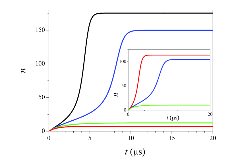
Figure 2: Time evolution of terahertz photons number at zero temperature for different pumps: $4500$ ps^-1 (red), $5000$ ps^-1 (green), $5500$ ps^-1 (blue) and $6000$ ps^-1 (black). Inset shows evolution of THz photons number for the constant pump $P=6$ $10^{3}$ ps^-1 for different temperatures: 1 K (red), 10 K (green) and 20 K (blue).

Equilibrium value of the THz population $n$ as a function of pumping $P$ demonstrates threshold-like behavior. For high enough temperatures, below the threshold the dependence of $n$ on $P$ is very weak. When pumping reaches the certain threshold value, polariton condensate is formed in the lower polariton state, radiative THz transition is amplified by bosonic stimulation, and the occupancy of THz mode increases superlinearly together with the occupancy of lower polariton state $n_{L}$ (Fig.2, blue curve). This behavior is qualitatively the same as in the approach operating with semiclassical Boltzmann equations. However, the decrease of temperature leads to the onset of the bistability and hysteresis in the dependence $n(P)$. The bistable jump occurs when the intensity of the pump tunes $\tilde{\epsilon}_{U}-\tilde{\epsilon}_{L}$ into the resonance with the cavity mode $\epsilon_{T}$. The parameters of the hysteresis loop strongly depend on the temperature (Fig.3). It is very pronounced and broad for low temperatures, narrows with the increase of the temperature and disappears completely at $T\approx 20K$.

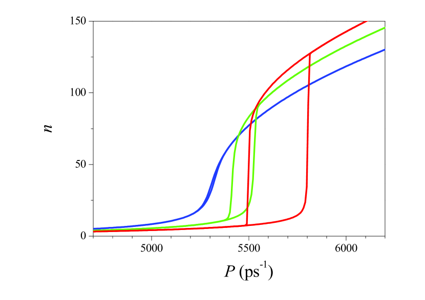
Figure 3: Dependence of occupancy of the THz mode on pump in equilibrium state for different temperatures: 1 K (red), 10 K (green) and 20 K (blue).

Coherent nature of the interaction beween excitons and THz photons makes possible the periodic exchange of the energy between polaritonic and photonic modes and oscillatory dependence of the THz signal in time. Fig.3 shows temporal evolution of the occupancy of THz mode after excitation of the upper polariton state by a short pulse having a duration of about 2 ps. It is seen that the occupancy of THz mode reveals a sequence of the short pulses having duration of dozens of ps with amplitude decaying in time due to escape of THz photons from a cavity and radiative decay of polaritons. The period of the oscillations is sensitive to the number of the injected polaritons $N_{0}$ and decreases with increasing of $N_{0}$. If the lifetime of polaritons is less than the period of the oscillations, single pulse behaviour can be observed as it is shown in the inset of Fig.4. Appropriate choice of the parameters can ultimately lead to a generation of THz wavelets composed of one or several THz cycles, which makes polariton-THz system suitable for application in a sort pulse THZ spectroscopy.

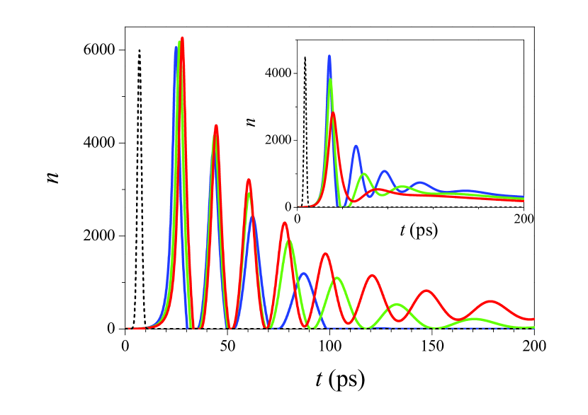
after the arrival of the short excitation pulse (dashed black line).

Figure 4: The temporal dependence of the terahertz mode occupancy. The background pump is switched off, lifetimes $\tau_{L}=\tau_{U}=50$ ps. The temperatures are: 1 K (red line), 10 K (green) and 20 K (blue). Inset: T=1K, different lifetimes of the polariton states: 15 ps (red), 20 ps(green) and 25 ps(blue).

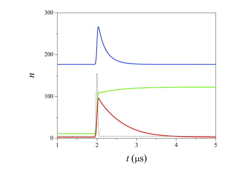
Figure 5: System response on a short single impuls (FWHM$=40$ ps, black/dotted curve) for different values of the background pump: 4600 ps^-1 (red), 5750 ps^-1 (green), 6500 ps^-1 (blue). Switching occurs only when the background pump corresponds to the bistable region (compare with Fig. 2).

If the system of coupled THz photons and cavity polaritons is in the state corresponding to the lower branch of the S-shaped curve in the bistability region, illumination of the system by a short THz impulse $I(t)$ can induce its switching to the upper branch, as it is demonstrated at Fig.5. One sees, that the response of the system is qualitatively different for different values of the pump $P$. If $P$ lies outside the bistablity region, the application of THz pulse leads to a short increase of the $n$ but subsequently the system relaxes to its original state (red and blue curves). However, when the system is in the bistability regime the switching occurs. Note that this effect is of quantum nature and cannot be describes using the approach based on semiclassical Boltzmann equations developed in Ref.Kavokin1, .

Conclusion. We considered the system of coupled cavity polaritons and THz photons using the approach based on generalized Lindblad equation for the density matrix. We showed that such system demonstrates a variety of intriguing nonlinear effects, including bistability, THz swithching and generation of short THz wavelets. The work was supported by Rannis ”Center of excellence in polaritonics”, FP7 IRSES ”POLAPHEN” and ”POLALAS” projects, Russian Fund of Basic Research and COST ”POLATOM” program.

I Supplementary materials

In the present supplementary appendix we present a derivation of the quantum kinetic equations for the system of cavity polaritons coupled with a terahertz (THz) cavity mode based on the Lindblad approach for the density matrix dynamics. The method we develop is general and can in principle be applied to any system of interacting bosons in contact with a phonon reservoir, for example, a polaritonic channel [18,19] or a condensate of indirect excitons.

I.1 The Lindblad approach

The system of polaritons, phonons and THz cavity photons is described by its density matrix $\rho$, for which we apply Born approximation factorizing it into the phonon part which is supposed to be time-independent and corresponds to the thermal distribution of acoustic phonons $\rho_{ph}=\texttt{exp}\left\{-\beta\widehat{H}_{ph}\right\}$, and the part describing polaritons and THz cavity photons $\rho_{cav}$ whose time dependence should be determined. $\rho=\rho_{ph}\otimes\rho_{cav}$. Our aim is to find dynamic equations for the time evolution of the occupancies of the upper and lower polariton states and the THz cavity mode:

$$n_{i}(t)=Tr\left\{\widehat{a}_{i}^{\dagger}\widehat{a}_{i}\rho(t)\right\}\equiv\langle\widehat{a}_{i}^{\dagger}\widehat{a}_{i}\rangle$$ (15)

where $\widehat{a}_{i}^{\dagger}$ and $\widehat{a}_{j}$ are operators of the upper and lower polaritons ($i=U$ and $i=L$ respectively) and THz cavity photons ($i=T$). In our consideration we neglect spin of the cavity polaritons since out goal is to find the effects of bistability and switching in the THz emitter and spin degree of freedom is not expected to introduce any qualitatively new physics from this point of view. It should be noted, however, that introduction of spin into the model is straightforward.

The total Hamiltonian of the system can be represented as a sum of two parts

$$\widehat{H}=\widehat{H}^{(1)}+\widehat{H}^{(2)}$$ (16)

where the first term $\widehat{H}^{(1)}$ describes the ”coherent” part of the evolution, corresponding to free polaritons, cavity photons and polariton-polariton interactions, and the second term $\widehat{H}^{(2)}$ corresponds to the dissipative interaction with acoustic phonons. The two terms affect the polariton density matrix in a qualitatively different way. The effect of the coherent part on the evolution of the density matrix is described by the Liouville-von Neumann equation

$$i\left(\partial_{t}\rho\right)^{(1)}=\left[\widehat{H}^{(1)};\widehat{\rho}\right]$$ (17)

Polariton-phonon scattering corresponds to the interaction of the quantum polariton system with a classical phonon reservoir. It is of dissipative nature, and thus straightforward application of the Liouville-von Neumann equation is impossible. Introduction of dissipation into quantum systems is an old problem, for which there is still no single well established solution. In the domain of quantum optics, however, there are standard methods based on the Master Equation techniques. In the following we give a brief outline of this approach applied for a dissipative polariton system.

The Hamiltonian of interaction of polaritons with acoustic phonons in Dirac representation can be represented as

$$\widehat{H}^{(2)}(t)=\widehat{H}^{-}(t)+\widehat{H}^{+}(t)=D_{U}\sum_{k}e^{i\left(E_{U}-E_{Rk}\right)t}\left(\widehat{a}_{U}\widehat{a}_{Rk}^{+}+\widehat{a}_{U}^{+}\widehat{a}_{Rk}\right)\left(\widehat{b}_{k}e^{-i\omega_{k}t}+\widehat{b}_{k}^{+}e^{i\omega_{k}t}\right)+$$ (18)

$$+D_{L}\sum_{k}e^{i\left(E_{Rk}-E_{L}\right)t}\left(\widehat{a}_{L}\widehat{a}_{Rk}^{+}+\widehat{a}_{L}^{+}\widehat{a}_{Rk}\right)\left(\widehat{b}_{k}e^{-i\omega_{k}t}+\widehat{b}_{k}^{+}e^{i\omega_{k}t}\right)$$

where $\widehat{a}_{i}$ are the operators for polaritons, $\widehat{b}_{k}$ are the operators for phonons, $E_{i}$ and $\omega_{k}$ are the dispersion relations of polaritons and acoustic phonons respectively, $D_{i}$ are the polariton-phonon coupling constants. In the last equality we separated the terms $\widehat{H}^{+}$ where a phonon is created, containing the operators $\widehat{b}^{+}$, from the terms $\widehat{H}^{-}$ in which it is destroyed, containing operators $\widehat{b}$.

Now, one can consider a hypothetical situation when polariton-polariton interactions are absent, and all redistributions of the polaritons are due to the scattering with a thermal reservoir of acoustic phonons. One can rewrite the Liouville-von Neumann equation in an integro-differential form and apply the so-called Markovian approximation

$$\left(\partial_{t}\rho\right)^{(2)}=-\frac{1}{\hbar^{2}}\int_{-\infty}^{t}\left[\widehat{H}^{(2)}(t);\left[\widehat{H}^{(2)}(t^{\prime});\widehat{\rho}(t)\right]\right]=$$ (19)

$$=\delta_{\Delta E}\left[2\left(\widehat{H}^{+}\widehat{\rho}\widehat{H}^{-}+\widehat{H}^{-}\widehat{\rho}\right.\widehat{H}^{+}\right)\left.-\left(\widehat{H}^{+}\widehat{H}^{-}+\widehat{H}^{-}\widehat{H}^{+}\right)\widehat{\rho}-\widehat{\rho}\left(\widehat{H}^{+}\widehat{H}^{-}+\widehat{H}^{-}\widehat{H}^{+}\right)\right]=\widehat{L}_{H^{(2)}}\rho,$$

where in the last line symbol $\widehat{L}_{H^{(2)}}$ denotes a Lindblad dissipative operator corresponding to the Hamiltonian $\widehat{H}^{(2)}$. The coefficient $\delta_{\Delta E}$ corresponds to the energy conservation and has dimensionality of inverse energy divided by square of a Plank constant. In calculations we estimate $\delta_{\Delta E}$ as being proportional to the inverse broadening of the polaritons states (as it is usually done in calculation of the transition rates in semiclassical Boltzmann equations using Fermi golden rule). For time evolution of the mean value of any arbitrary operator $\langle\widehat{A}\rangle=Tr(\rho\widehat{A})$ due to scattering with phonons one thus has:

$$\left\{\partial_{t}\langle\widehat{A}\rangle\right\}^{(2)}=\delta_{\Delta E}\left(\langle[\widehat{H}^{-};[\widehat{A};\widehat{H}^{+}]]\rangle+\langle[\widehat{H}^{+};[\widehat{A};\widehat{H}^{-}]]\rangle\right).$$ (20)

Putting $\widehat{A}=\widehat{a}_{i}^{+}\widehat{a}_{i}$ in this equation we get the contributions to the dynamic equations for the occupancies coming from polariton-phonon interactions, which are nothing more than the standard semi-classical Boltzmann equations describing the thermalization of a polariton system.

Combined together, coherent and incoherent contributions result in a following master equation for the density matrix:

$$\frac{\partial\rho}{\partial t}=\frac{i}{\hbar}[\widehat{\rho};\widehat{H}^{(1)}]+\widehat{L}_{H^{(2)}}\rho$$ (21)

I.2 Coherent part

Let us consider the coherent part. Hamiltonian here $\widehat{H}^{(1)}=\widehat{H}_{0}+\widehat{H}_{T}+\widehat{H}_{pol-pol}$ (let us omit symbols ” $\widehat{}$ ” over operators hereafter.), where

$$H_{0}=\epsilon_{L}a_{L}^{+}a_{L}+\epsilon_{U}a_{U}^{+}a_{U}+\epsilon_{T}c^{+}c$$ (22)

is the free-polariton Hamiltonian,

$$H_{T}=V_{T}\left(a_{U}^{+}a_{L}c+a_{U}a_{L}^{+}c^{+}\right)$$ (23)

is the polaritons-to-THz photons interaction term and

$$H_{pol-pol}=U_{LL}a_{L}^{+}a_{L}^{+}a_{L}a_{L}+U_{UU}a_{U}^{+}a_{U}^{+}a_{U}a_{U}+2U_{UL}a_{U}^{+}a_{U}a_{L}^{+}a_{L}+2U_{UR}\sum_{k}{a_{U}^{+}a_{U}a_{Rk}^{+}a_{Rk}}+2U_{LR}\sum_{k}{a_{L}^{+}a_{L}a_{Rk}^{+}a_{Rk}}\approx$$ (24)

$$\approx 2\left[U_{LL}(a_{L}^{+}a_{L}\langle a_{L}^{+}a_{L}\rangle)+U_{UU}\left(a_{U}^{+}a_{U}\langle a_{U}^{+}a_{U}\rangle\right)+U_{UL}\left(a_{L}^{+}a_{L}\langle a_{U}^{+}a_{U}\rangle\right)+U_{UL}\left(a_{U}^{+}a_{U}\langle a_{L}^{+}a_{L}\rangle\right)+\right.$$

$$\left.+U_{UR}\left(a_{U}^{+}a_{U}\langle a_{Rk}^{+}a_{Rk}\rangle\right)+U_{UR}\left(a_{Rk}^{+}a_{Rk}\langle a_{U}^{+}a_{U}\rangle\right)+U_{LR}\left(a_{L}^{+}a_{L}\langle a_{Rk}^{+}a_{Rk}\rangle\right)+U_{LR}\left(a_{Rk}^{+}a_{Rk}\langle a_{L}^{+}a_{L}\rangle\right)\right]\approx$$

$$\approx 2\left(U_{LL}n_{L}+U_{UL}n_{U}+\sum_{k}{U_{LR}n_{Rk}}\right)a_{L}^{+}a_{L}+2\left(U_{UU}n_{U}+U_{UL}n_{L}+\sum_{K}{U_{UR}n_{Rk}}\right)a_{U}^{+}a_{U}+$$

$$+2\left(U_{UR}n_{U}+U_{LR}n_{L}\right)\sum_{k}{a_{Rk}^{+}a_{Rk}}=U_{1}a_{L}^{+}a_{L}+U_{2}a_{U}^{+}a_{U}+U_{3}\sum_{k}{a_{Rk}^{+}a_{Rk}};$$

is the polariton-polariton scattering Hamiltonian. Coming from the first to the second lines of this expression we used mean-field approximation. Here we also introduced three new coefficients:

$$U_{1}=2\left(U_{LL}n_{L}+U_{UL}n_{U}+\sum_{k}{U_{LR}n_{Rk}}\right),$$ (25)

$$U_{2}=2\left(U_{UU}n_{U}+U_{UL}n_{L}+\sum_{K}{U_{UR}n_{Rk}}\right),$$ (26)

$$U_{3}=2\left(U_{UR}n_{U}+U_{LR}n_{L}\right).$$ (27)

1) Lower and upper polaritons occupancies $n_{L},n_{U}$,

Consider the dynamic equation for $n_{L}$ as an example. One has

$$\hbar\left(\partial_{t}n_{L}\right)^{(1)}=i\textrm{Tr}\{a_{L}^{+}a_{L}[\rho;H^{(1)}]\};$$

$$\hbar\left(\partial_{t}n_{L}\right)_{0}=i\textrm{Tr}\{a_{L}^{+}a_{L}[\rho;H_{0}]\}=i\textrm{Tr}\{\rho[\epsilon_{L}a_{L}^{+}a_{L}+\epsilon_{U}a_{U}^{+}a_{U}+\epsilon_{T}c^{+}c;a_{L}^{+}a_{L}]\}=0;$$

$$\hbar\left(\partial_{t}n_{L}\right)_{T}=iV_{T}\textrm{Tr}\{\rho[a_{U}^{+}a_{L}c+a_{U}a_{L}^{+}c^{+};a_{L}^{+}a_{L}]\}=iV_{T}\left(a_{UL}-a_{UL}^{+}\right)=-2V_{T}\textrm{Im}\left(a_{UL}\right);$$

$$\hbar\left(\partial_{t}n_{L}\right)_{pol-pol}=i\textrm{Tr}\{\rho[U_{1}a_{L}^{+}a_{L}+U_{2}a_{U}^{+}a_{U}+U_{3}\sum_{k}{a_{Rk}^{+}a_{Rk}};a_{L}^{+}a_{L}]\}=0.$$

Finally,

$$\hbar\left(\partial_{t}n_{L}\right)^{(1)}=-2V_{T}\textrm{Im}\left(a_{UL}\right).$$ (28)

The equation for the upper polariton occupancy is obtained in a similar way.

2) Reservoir $n_{Rk}$,

$$\hbar\left(\partial_{t}n_{Rk}\right)^{(1)}=i\textrm{Tr}\{a_{Rk}^{+}a_{Rk}[\rho;H^{(1)}]\}=0.\\$$ (29)

3) Terahertz cavity occupancy $n_{T}$,

$$\hbar\left(\partial_{t}n_{T}\right)^{(1)}=i\textrm{Tr}\{c^{+}c[\rho;H^{(1)}]\};$$

$$\hbar\left(\partial_{t}n_{T}\right)_{0}=i\textrm{Tr}\{c^{+}c[\rho;H_{0}]\}=0;$$

$$\hbar\left(\partial_{t}n_{T}\right)_{T}=iV_{T}\textrm{Tr}\{\rho[a_{U}^{+}a_{U}c+a_{U}a_{L}^{+};c^{+}c]\}=iV_{T}\left(a_{UL}-a_{UL}^{+}\right)=-2V_{T}\textrm{Im}\left(a_{UL}\right);$$

$$\hbar\left(\partial_{t}n_{T}\right)_{pol-pol}=i\textrm{Tr}\{\rho[U_{1}a_{L}^{+}a_{L}+U_{2}a_{U}^{+}a_{U}+U_{3}\sum_{k}{a_{Rk}^{+}a_{Rk}};c^{+}c]\}=0.$$

Finally,

$$\hbar\left(\partial_{t}n_{T}\right)^{(1)}=-2V_{T}\textrm{Im}\left(a_{UL}\right).\\$$ (30)

4) Correlators $a_{UL}$,

$$\hbar\left(\partial_{t}a_{UL}\right)^{(1)}=i\textrm{Tr}\{a_{U}^{+}a_{L}c[\rho;H^{(1)}]\};$$

$$\hbar\left(\partial_{t}a_{UL}\right)_{0}=i\textrm{Tr}\{a_{U}^{+}a_{L}c[\rho;H_{0}]\}=i\textrm{Tr}\{\rho[\epsilon_{L}a_{L}^{+}a_{L}+\epsilon_{U}a_{U}^{+}a_{U}+\epsilon_{T}c^{+}c;a_{U}^{+}a_{L}c]\}=i\left(-\epsilon_{L}+\epsilon_{U}-\epsilon_{T}\right)a_{UL};$$

$$\hbar\left(\partial_{t}a_{UL}\right)_{T}=iV_{T}\textrm{Tr}\{\rho[a_{U}^{+}a_{L}c+a_{U}a_{L}^{+}c^{+};a_{U}^{+}a_{L}c]\}=iV_{T}\left(\langle a_{U}a_{L}^{+}a_{U}^{+}a_{L}c^{+}c\rangle-\langle a_{U}^{+}a_{L}a_{U}a_{L}^{+}cc^{+}\rangle\right)=$$

$$=-iV_{T}\{\left(n_{U}+1\right)n_{L}n_{T}-n_{U}\left(n_{L}+1\right)\left(n_{T}+1\right)\};$$

$$\hbar\left(\partial_{t}a_{UL}\right)_{pol-pol}=i\textrm{Tr}\{\rho[U_{1}a_{L}^{+}a_{L}+U_{2}a_{U}^{+}a_{U}+U_{3}\sum_{k}{a_{Rk}^{+}a_{Rk}};a_{U}^{+}a_{L}c]\}=$$

$$=iU_{1}\textrm{Tr}\{\rho[a_{L}^{+}a_{L};a_{U}^{+}a_{L}c]\}+iU_{2}\textrm{Tr}\{[a_{U}^{+}a_{U};a_{U}^{+}a_{L}c]\}=iU_{1}\left(-a_{UL}\right)+iU_{2}a_{UL}.$$

Finally,

$$\hbar\left(\partial_{t}a_{UL}\right)^{(1)}=i\left(\epsilon_{U}-\epsilon_{L}-\epsilon_{T}\right)a_{UL}+2V_{T}\{\left(n_{U}+1\right)n_{L}n_{T}-$$ (31)

$$n_{U}\left(n_{L}+1\right)\left(n_{T}+1\right)\}+i\{2U_{UU}n_{U}+U_{UL}\left(n_{L}-n_{U}\right)-2U_{LL}n_{L}+\left(U_{UR}-U_{LR}\right)\sum_{k}{n_{Rk}}\}a_{UL};$$

I.3 Decoherent part

To get explicit expresions for the dynamics of $n_{L}$, $n_{U}$, $n_{Rk}$, $n_{T}$ and $a_{UL}$ due to decoherent processes of interaction with the reservoir let us consider Liouville-von Neumann equation for the density matrix after the Born-Markov approximation Eq. (6) and the simplest case when only three states $L$, $U$ and $R_{k}$ are present.

In this case, leaving energy- conserving terms only one gets

$$H^{+}=D_{1}\sum_{k}a_{U}a_{kR}^{+}b_{k}^{+}+D_{2}\sum_{k}a_{L}^{+}a_{kR}b_{k}^{+}$$ (32)

$$H^{-}=D_{1}\sum_{k}a_{U}^{+}a_{kR}b_{k}+D_{2}\sum_{k}a_{L}a_{kR}^{+}b_{k}$$ (33)

The application of Eq. (6) gives the following results:

1) Lower and upper branch polariton occupancies $n_{L},n_{U}$,

For $n_{L}$ one has:

$$\left(\partial_{t}n_{L}\right)^{(2)}=\delta_{\Delta E}\left([H^{-};[a_{L}^{+}a_{L};H^{+}]]+[H^{+};[a_{L}^{+}a_{L};H^{-}]]\right)=2\delta_{\Delta E}[H^{+};[a_{L}^{+}a_{L};H^{-}]];$$

$$[a_{L}^{+}a_{L};H^{-}]=[a_{L}^{+}a_{L};D_{1}\sum_{k}a_{U}^{+}a_{Rk}b_{k}+D_{2}\sum_{k}a_{L}a_{Rk}^{+}b_{k}]=-D_{2}\sum_{k}a_{L}a_{Rk}^{+}b_{k};$$

$$[H^{+};[a_{L}^{+}a_{L};H^{-}]]=[D_{1}\sum_{k}a_{U}a_{Rk}^{+}b_{k}^{+}+D_{2}\sum_{k}a_{L}^{+}a_{Rk}b_{k}^{+};-D_{2}\sum_{k}a_{L}a_{Rk}^{+}b_{k}]=$$

$$[D_{2}\sum_{k}a_{L}^{+}a_{Rk}b_{k}^{+};-D_{2}\sum_{k}a_{L}a_{Rk}^{+}b_{k}]=D_{2}^{2}\sum_{k}\{\left(a_{L}^{+}a_{L}+1\right)a_{Rk}^{+}a_{Rk}\left(b_{k}^{+}b_{k}+1\right)-a_{L}^{+}a_{L}\left(a_{Rk}^{+}a_{Rk}+1\right)b_{k}^{+}b_{k}\};$$

Finally,

$$\hbar^{2}(\partial_{t}n_{L})^{(2)}=W_{2}\sum_{k}\{\left(n_{L}+1\right)n_{Rk}\left(n_{k}^{ph}+1\right)-n_{L}\left(n_{Rk}+1\right)n_{k}^{ph}\},$$ (34)

where we introduced $W_{2}=2\delta_{\Delta E}D_{2}^{2}$.

The equation for $n_{U}$ is easily obtained in an analogical way.

2) Reservoir $n_{Rk}=\langle a_{Rk}^{+}a_{Rk}\rangle$,

$$\left(\partial_{t}n_{Rk}\right)^{(2)}=2\delta_{\Delta E}[H^{+};[a_{Rk}^{+}a_{Rk};H^{-}]];$$

$$[a_{Rk}^{+}a_{Rk};H^{-}]=[a_{Rk}^{+}a_{Rk};D_{1}\sum_{k}a_{U}^{+}a_{Rk}b_{k}+D_{2}\sum_{k}a_{L}a_{Rk}^{+}b_{k}]=-D_{1}\sum_{k}a_{U}^{+}a_{Rk}b_{k}+D_{2}\sum_{k}a_{L}a_{Rk}^{+}b_{k};$$

$$[H^{+}[a_{Rk}^{+}a_{Rk};H^{-}]]=[D_{1}\sum_{k}a_{U}a_{Rk}^{+}b_{k}^{+}+D_{2}\sum_{k}a_{L}^{+}a_{Rk}b_{k}^{+};-D_{1}\sum_{k}a_{U}^{+}a_{Rk}b_{k}+D_{2}\sum_{k}a_{L}a_{Rk}^{+}b_{k}]\approx$$

$$\approx D_{1}^{2}\sum_{k}\{a_{U}^{+}a_{U}\left(a_{Rk}^{+}a_{Rk}+1\right)\left(b_{k}^{+}b_{k}+1\right)-\left(a_{U}^{+}a_{U}+1\right)a_{Rk}^{+}a_{Rk}b_{k}^{+}b_{k}\}+$$

$$+D_{2}^{2}\sum_{k}\{a_{L}^{+}a_{L}\left(a_{Rk}^{+}a_{Rk}+1\right)b_{k}^{+}b_{k}-\left(a_{L}^{+}a_{L}+1\right)a_{Rk}^{+}a_{Rk}\left(b_{k}^{+}b_{k}+1\right)\},$$

where coming between the third and the fourth lines we neglected the off- diaginal elements of the phonon density matrix, supposing $\langle b_{k}^{+}b_{k^{\prime}}\rangle=n^{ph}_{k}\delta_{k,k^{\prime}}$

Finally,

$$(\partial_{t}n_{Rk})^{(2)}\approx W_{1}\sum_{k}\{n_{U}\left(n_{Rk}+1\right)\left(n_{k}^{ph}+1\right)-\left(n_{U}+1\right)n_{Rk}n_{k}^{ph}\}+$$ (35)

$$+W_{2}\sum_{k}\{n_{L}\left(n_{Rk}+1\right)n_{k}^{ph}-\left(n_{L}+1\right)n_{Rk}\left(n_{k}^{ph}+1\right)\}.$$

3) Terahertz cavity occupancy $n_{T}=\langle c^{+}c\rangle$,

$$\left(\partial_{t}n_{T}\right)^{(2)}=\delta_{\Delta E}\left([H^{-};[c^{+}c;H^{+}]]+[H^{+};[c^{+}c;H^{-}]]\right)=0.\\$$ (36)

4) Decoherent part of the correlator $a_{UL}=\langle a_{U}^{+}a_{L}c\rangle$,

$$[a_{U}^{+}a_{L}c;H^{-}]=0;$$

$$[a_{U}^{+}a_{L}c;H^{+}]=[a_{U}^{+}a_{L}c;D_{1}\sum_{k}a_{U}a_{Rk}^{+}b_{k}^{+}+D_{2}\sum_{k}a_{L}^{+}a_{Rk}b_{k}^{+}]=-\sum_{k}D_{1}a_{Rk}^{+}a_{L}cb_{k}^{+}+D_{2}\sum_{k}a_{U}^{+}a_{Rk}cb_{k}^{+};$$

$$[H^{-};[a_{U}^{+}a_{L}c;H^{+}]]=[D_{1}\sum_{k}a_{U}^{+}a_{Rk}b_{k}+D_{2}\sum_{k}a_{L}a_{Rk}^{+}b_{k};-D_{1}\sum_{k}a_{Rk}^{+}a_{L}cb_{k}^{+}+D_{2}\sum_{k}a_{U}^{+}a_{Rk}cb_{k}^{+}]\approx$$

$$\approx D_{1}^{2}\sum_{k}\{a_{Rk}^{+}a_{Rk}\left(a_{U}^{+}a_{L}c\right)b_{k}^{+}b_{k}-\left(a_{Rk}^{+}a_{Rk}+1\right)a_{U}^{+}a_{L}c\left(b_{k}^{+}b_{k}+1\right)\}+$$

$$+D_{2}^{2}\sum_{k}\{a_{Rk}^{+}a_{Rk}a_{U}^{+}a_{L}c\left(b_{k}^{+}b_{k}+1\right)-\left(a_{Rk}^{+}a_{Rk}+1\right)a_{U}^{+}a_{L}cb_{k}^{+}b_{k}\}=$$

$$=D_{1}^{2}\sum_{k}\{-a_{Rk}^{+}a_{Rk}a_{U}^{+}a_{L}c-a_{U}^{+}a_{L}c\left(b_{k}^{+}b_{k}+1\right)\}+D_{2}^{2}\sum_{k}\{a_{Rk}^{+}a_{Rk}a_{U}^{+}a_{L}c-a_{U}^{+}a_{L}cb_{k}^{+}b_{k}\}.$$

Finally,

$$(\partial_{t}a_{UL})^{(2)}=\frac{W_{1}}{2}\sum_{k}\left(-n_{Rk}-n_{k}^{ph}-1\right)a_{UL}+\frac{W_{2}}{2}\sum_{k}\left(n_{Rk}-n_{k}^{ph}\right)a_{UL}.\\$$ (37)

After merging the equations for the coherent processes with the equations for the incoherent phonon-scattering processes and adding finite lifetimes, background and impulse pumps (see main text of the Letter) we solve this self-consistent set of equations and eventually find the evolution of the THz photons occupancy.

References

• (1) G. Davies et al, Physics World 17, 37 (2004)
• (2) H. T. Duc et al, Phys. Rev. B 74, 165328 (2006)
• (3) T. D. Doan et al, Phys. Rev. B 72, 085301 (2005)
• (4) Y. Todorov et al, Phys. Rev. Lett. 99, 223603 (2007)
• (5) Y. Chassagneux et al, Nature 457, 174-178 (2009)
• (6) K. V. Kavokin et al, Appl. Phys. Lett. 97, 201111 (2010)
• (7) A. Amo et al, Nature 457, 291 (2009).
• (8) A. Baas et al, Phys. Rev. B 70, 161307(R) (2004).
• (9) N. A. Gippius et al, Phys. Rev. Lett. 98, 236401 (2007).
• (10) O. A. Egorov et al, Phys. Rev. B 82, 165326 (2010)
• (11) Y. Todorov et al, Phys. Rev. Lett. 105, 196402 (2010)
• (12) G. Gunter et al, Nature 458 178 (2009)
• (13) F. Junginger et al, Opt.Lett. 35(15) 2645 (2010)
• (14) Y. Todorov et al, Phys. Rev. Lett 102, 186402 (2009)
• (15) S. De Liberato, C. Ciuti, Phys. Rev. Lett. 102, 136403 (2009)
• (16) D. Oustinov et al, Nature Communication 1 69 (2010)
• (17) M. Swoboda et al, Appl. Phys. Lett. 89, 121110 (2006)
• (18) C. Ciuti et al, Phys. Rev. B 58, 7926 (1998).
• (19) M.O Scully and M.A. Zubairy, Quantum Optics, Cambridge University Press, 1997
• (20) E. B. Magnusson et al, Phys. Rev. B 82, 195312 (2010)
• (21) I. G. Savenko et al, Phys. Rev. B 83, 165316 (2011)
• (22) Y. Chassagneux et al, Nature 457(7226), 174-178 (2009)
• (23) A. J. Gallant et al, Appl. Phys. Lett. 91, 161115 (2007)