New efficient estimation and variable selection methods for semiparametric varying-coefficient partially linear models

Abstract

The complexity of semiparametric models poses new challenges to statistical inference and model selection that frequently arise from real applications. In this work, we propose new estimation and variable selection procedures for the semiparametric varying-coefficient partially linear model. We first study quantile regression estimates for the nonparametric varying-coefficient functions and the parametric regression coefficients. To achieve nice efficiency properties, we further develop a semiparametric composite quantile regression procedure. We establish the asymptotic normality of proposed estimators for both the parametric and nonparametric parts and show that the estimators achieve the best convergence rate. Moreover, we show that the proposed method is much more efficient than the least-squares-based method for many non-normal errors and that it only loses a small amount of efficiency for normal errors. In addition, it is shown that the loss in efficiency is at most $11.1\%$ for estimating varying coefficient functions and is no greater than $13.6\%$ for estimating parametric components. To achieve sparsity with high-dimensional covariates, we propose adaptive penalization methods for variable selection in the semiparametric varying-coefficient partially linear model and prove that the methods possess the oracle property. Extensive Monte Carlo simulation studies are conducted to examine the finite-sample performance of the proposed procedures. Finally, we apply the new methods to analyze the plasma beta-carotene level data.

, and

t1Supported by NIDA, NIH Grants R21 DA024260 and P50 DA10075. t2Supported by NNSF of China Grant 11028103, NSF Grant DMS-03-48869 and NIDA, NIH Grants R21 DA024260. The content is solely the responsibility of the authors and does not necessarily represent the official views of the NIDA or the NIH. t3Supported by NSF Grant DMS-08-46068.

1 Introduction

Semiparametric regression modeling has recently become popular in the statistics literature because it keeps the flexibility of nonparametric models while maintaining the explanatory power of parametric models. The partially linear model, the most commonly used semiparametric regression model, has received a lot of attention in the literature; see Härdle, Liang and Gao HardleLiangGao2000 , Yatchew Yatchew2003 and references therein for theory and applications of partially linear models. Various extensions of the partially linear model have been proposed in the literature; see Ruppert, Wand and Carroll RuppertWandCarroll2003 for applications and theoretical developments of semiparametric regression models. The semiparametric varying-coefficient partially linear model, as an important extension of the partially linear model, is becoming popular in the literature. Let $Y$ be a response variable and $\{U,\mathbf{X},\mathbf{Z}\}$ its covariates. The semiparametric varying-coefficient partially linear model is defined to be

$$Y=\alpha_{0}(U)+\mathbf{X}^{T}{\bolds{\alpha}}(U)+\mathbf{Z}^{T}{\bolds{\beta}}+\varepsilon,$$ (1)

where $\alpha_{0}(U)$ is a baseline function, ${\bolds{\alpha}}(U)=\{\alpha_{1}(U),\ldots,\alpha_{d_{1}}(U)\}^{T}$ consists of $d_{1}$ unknown varying coefficient functions, ${\bolds{\beta}}=(\beta_{1},\ldots,\beta_{d_{2}})^{T}$ is a $d_{2}$-dimensional coefficient vector and $\varepsilon$ is random error. In this paper, we will focus on univariate $U$ only, although the proposed procedure is directly applicable for multivariate $\mathbf{U}$. Zhang, Lee and Song ZhangLeeSong2002 proposed an estimation procedure for the model (1), based on local polynomial regression techniques. Xia, Zhang and Tong XiaZhangTong2004 proposed a semilocal estimation procedure to further reduce the bias of the estimator for ${\bolds{\beta}}$ suggested in Zhang, Lee and Song ZhangLeeSong2002 . Fan and Huang FanHuang2005 proposed a profile least-squares estimator for model (1) and developed statistical inference procedures. As an extension of Fan and Huang FanHuang2005 , a profile likelihood estimation procedure was developed in Lam and Fan LamFan2008 , under the generalized linear model framework with a diverging number of covariates.

Existing estimation procedures for model (1) were built on either least-squares- or likelihood-based methods. Thus, the existing procedures are expected to be sensitive to outliers and their efficiency may be significantly improved for many commonly used non-normal errors. In this paper, we propose new estimation procedures for model (1). This paper contains three major developments: (a) semiparametric quantile regression; (b) semiparametric composite quantile regression; (c) adaptive penalization methods for achieving sparsity in semiparametric composite quantile regression.

Quantile regression is often considered as an alternative to least-squares in the literature. For a complete review on quantile regression, see Koenker Koenker2005 . Quantile-regression-based inference procedures have been considered in the literature; see, for example, Cai and Xu CaiXu08 , He and Shi HeShi1996 , He, Zhu and Fung HeZhuFung2002 , Lee Lee2003 , among others. In Section 2, we propose a new semiparametric quantile regression procedure for model (1). We investigate the sampling properties of the proposed method and their asymptotic normality. When applying semiparametric quantile regression to model (1), we observe that all quantile regression estimators can estimate ${\bolds{\alpha}}(u)$ and ${\bolds{\beta}}$ with the optimal rate of convergence. This fact motivates us to combine the information across multiple quantile estimates to obtain improved estimates of ${\bolds{\alpha}}(u)$ and ${\bolds{\beta}}$. Such an idea has been studied for the parametric regression model in Zou and Yuan ZouYuan2008 and it leads to the composite quantile regression (CQR) estimator that is shown to enjoy nice asymptotic efficiency properties compared with the classical least-squares estimator. In Section 3, we propose the semiparametric composite quantile regression (semi-CQR) estimators for estimating both nonparametric and parametric parts in model (1). We show that the semi-CQR estimators achieve the best convergence rates. We also prove the asymptotic normality of the semi-CQR estimators. The asymptotic theory shows that, compared with the semiparametric least-squares estimators, the semi-CQR estimators can have substantial efficiency gain for many non-normal errors and only lose a small amount of efficiency for normal errors. Moreover, the relative efficiency is at least $88.9\%$ for estimating varying-coefficient functions and is at least $86.4\%$ for estimating parametric components.

In practice, there are often many covariates in the parametric part of model (1). With high-dimensional covariates, sparse modeling is often considered superior, owing to enhanced model predictability and interpretability FanLi2006 . Variable selection for model (1) is challenging because it involves both nonparametric and parametric parts. Traditional variable selection methods, such as stepwise regression or best subset variable selection, do not work effectively for the semiparametric model because they need to choose smoothing parameters for each submodel and cannot cope with high-dimensionality. In Section 4, we develop an effective variable selection procedure to select significant parametric components in model (1). We demonstrate that the proposed procedure possesses the oracle property, in the sense of Fan and Li FanLi2001 .

In Section 5, we conduct simulation studies to examine the finite-sample performance of the proposed procedures. The proposed methods are illustrated with the plasma beta-carotene level data. Regularity conditions and technical proofs are given in Section 6.

2 Semiparametric quantile regression

In this section, we develop the semiparametric quantile regression method and theory. Let $\rho_{\tau}(r)=\tau r-rI$ $(r<0)$ be the check loss function at $\tau\in(0,1)$. Quantile regression is often used to estimate the conditional quantile functions of $Y$,

$$Q_{\tau}(u,\mathbf{x},\mathbf{z})=\operatorname{argmin}\limits_{a}E\{\rho_{\tau}(Y-a)|(U,\mathbf{X},\mathbf{Z})=(u,\mathbf{x},\mathbf{z})\}.$$

The semiparametric varying-coefficient partially linear model assumes that the conditional quantile function is expressed as $Q_{\tau}(u,\mathbf{x},\mathbf{z})=\alpha_{0,\tau}(u)+\mathbf{x}^{T}{\bolds{\alpha}}_{\tau}(u)+\mathbf{z}^{T}{\bolds{\beta}}_{\tau}.$

Suppose that $\{U_{i},\mathbf{X}_{i},\mathbf{Z}_{i},Y_{i}\}$, $i=1,\ldots,n,$ is an independent and identically distributed sample from the model

$$Y=\alpha_{0,\tau}(U)+\mathbf{X}^{T}{\bolds{\alpha}}_{\tau}(U)+\mathbf{Z}^{T}{\bolds{\beta}}_{\tau}+\varepsilon_{\tau},$$ (2)

where $\varepsilon_{\tau}$ is random error with conditional $\tau$th quantile being zero. We obtain quantile regression estimates of $\alpha_{0,\tau}(\cdot)$, ${\bolds{\alpha}}_{\tau}(\cdot)$ and ${\bolds{\beta}}_{\tau}$ by minimizing the quantile loss function

$$\sum_{i=1}^{n}\rho_{\tau}\{Y_{i}-\alpha_{0}(U_{i})-\mathbf{X}_{i}^{T}{\bolds{\alpha}}(U_{i})-\mathbf{Z}_{i}^{T}{\bolds{\beta}}\}.$$ (3)

Because (3) involves both nonparametric and parametric components, and because they can be estimated by different rates of convergence, we propose a three-stage estimation procedure. In the first stage, we employ local linear regression techniques to derive an initial estimates of $\alpha_{0,\tau}(\cdot)$, ${\bolds{\alpha}}_{\tau}(\cdot)$ and ${\bolds{\beta}}_{\tau}$. Then, in the second and third stages, we further improve the estimation efficiency of the initial estimates for ${\bolds{\beta}}_{\tau}$ and $(\alpha_{0,\tau}(\cdot),{\bolds{\alpha}}_{\tau}(\cdot))$, respectively.

For $U$ in the neighborhood of $u$, we use a local linear approximation

$$\alpha_{j}(U)\approx\alpha_{j}(u)+\alpha^{\prime}_{j}(u)(U-u)\triangleq a_{j}+b_{j}(U-u)$$

for $j=0,\ldots,d_{1}$. Let $\{{\tilde{a}}_{0,\tau},{\tilde{b}}_{0,\tau},{\tilde{\mathbf{a}}}_{\tau},{\tilde{\mathbf{b}}}_{\tau},{\tilde{{\bolds{\beta}}}}_{\tau}\}$ be the minimizer of the local weighted quantile loss function

$$\sum_{i=1}^{n}\rho_{\tau}\bigl{\{}Y_{i}-a_{0}-b_{0}(U_{i}-u)-\mathbf{X}_{i}^{T}\{\mathbf{a}+\mathbf{b}(U_{i}-u)\}-\mathbf{Z}_{i}^{T}{\bolds{\beta}}\bigr{\}}K_{h}(U_{i}-u),$$

where $\mathbf{a}=(a_{1},\ldots,a_{d_{1}})^{T}$, $\mathbf{b}=(b_{1},\ldots,b_{d_{1}})^{T}$, $K(\cdot)$ is a given kernel function and $K_{h}(\cdot)=K(\cdot/h)/h$ with a bandwidth $h$. Then,

$${\tilde{\alpha}}_{0,\tau}(u)={\tilde{a}}_{0},\qquad{\tilde{{\bolds{\alpha}}}}_{\tau}(u)={\tilde{\mathbf{a}}}_{\tau}.$$

We take $\{\tilde{\alpha}_{0,\tau}(u),\tilde{\bolds{\alpha}}_{\tau}(u),\tilde{\bolds{\beta}}_{\tau}\}$ as the initial estimates.

We now provide theoretical justifications for the initial estimates. First, we give some notation. Let $f_{\tau}(\cdot|u,\mathbf{x},\mathbf{z})$ and $F_{\tau}(\cdot|u,\mathbf{x},\mathbf{z})$ be the density function and cumulative distribution function of the error conditional on $(U,\mathbf{X},\mathbf{Z})=(u,\mathbf{x},\mathbf{z})$, respectively. Denote by $f_{U}(\cdot)$ the marginal density function of the covariate $U$. The kernel $K(\cdot)$ is chosen as a symmetric density function and we let

$$\mu_{j}=\int u^{j}K(u)\,du\quad\mbox{and}\quad\nu_{j}=\int u^{j}K^{2}(u)\,du,\qquad j=0,1,2,\ldots.$$

We then have the following result.

Theorem 2.1

Under the regularity conditions given in Section 7, if $h\rightarrow 0$ and $nh\rightarrow\infty$ as $n\rightarrow\infty$, then

$$\sqrt{nh}\left[\pmatrix{\tilde{\alpha}_{0,\tau}(u)-\alpha_{0,\tau}(u)\vspace*{3pt}\cr\tilde{\bolds{\alpha}}_{\tau}(u)-{\bolds{\alpha}}_{\tau}(u)\vspace*{3pt}\cr\tilde{\bolds{\beta}}_{\tau}-{\bolds{\beta}}_{\tau}}-\frac{\mu_{2}h^{2}}{2}\pmatrix{\alpha^{\prime\prime}_{0,\tau}(u)\vspace*{3pt}\cr{\bolds{\alpha}}^{\prime\prime}_{\tau}(u)\vspace*{2pt}\cr\mathbf{0}}\right]$$

(4)

$$\qquad\stackrel{{\scriptstyle\mathcal{D}}}{{\longrightarrow}}N\biggl{(}\mathbf{0},\frac{\nu_{0}\tau(1-\tau)}{f_{U}(u)}\mathbf{A}_{1}^{-1}(u)\mathbf{B}_{1}(u)\mathbf{A}_{1}^{-1}(u)\biggr{)},$$

where $\mathbf{A}_{1}(u)=E[f_{\tau}(0|U,\mathbf{X},\mathbf{Z})(1,\mathbf{X}^{T},\mathbf{Z}^{T})^{T}(1,\mathbf{X}^{T},\mathbf{Z}^{T})|U=u]$ and $\mathbf{B}_{1}(u)=E[(1,\mathbf{X}^{T},\mathbf{Z}^{T})^{T}(1,\mathbf{X}^{T},\mathbf{Z}^{T})|U=u]$.

Theorem 2.1 implies that $\tilde{\bolds{\beta}}_{\tau}$ is a $\sqrt{nh}$-consistent estimator—this is because we only use data in a local neighborhood of $u$ to estimate ${\bolds{\beta}}_{\tau}$. Define $Y_{i,\tau}^{*}=Y_{i}-\tilde{\alpha}_{0,\tau}(U_{i})-\mathbf{X}_{i}^{T}\tilde{\bolds{\alpha}}_{\tau}(U_{i})$ and compute an improved estimator of ${\bolds{\beta}}_{\tau}$ by

$$\hat{{\bolds{\beta}}}_{\tau}=\operatorname{argmin}\limits_{{\bolds{\beta}}}\sum_{i=1}^{n}\rho_{\tau}(Y_{i,\tau}^{*}-\mathbf{Z}_{i}^{T}{\bolds{\beta}}).$$ (5)

We call it the semi-QR estimator of ${\bolds{\beta}}_{\tau}$. The next theorem shows the asymptotic properties of $\hat{\bolds{\beta}}_{\tau}$.

Theorem 2.2

Let $\bolds{\xi}_{\tau}(u,\mathbf{x},\mathbf{z})=E[f_{\tau}(0|U,\mathbf{X},\mathbf{Z})\mathbf{Z}(1,\mathbf{X}^{T},\mathbf{0})|U=u]\times\break\mathbf{A}_{1}^{-1}(u)(1,\mathbf{x}^{T},\mathbf{z}^{T})^{T}$. Under the regularity conditions given in Section 7, if $nh^{4}\rightarrow 0$ and $nh^{2}/\log(1/h)\rightarrow\infty$ as $n\rightarrow\infty$, then the asymptotic distribution of $\hat{\bolds{\beta}}_{\tau}$ is given by

$$\sqrt{n}(\hat{\bolds{\beta}}_{\tau}-{\bolds{\beta}}_{\tau})\stackrel{{\scriptstyle\mathcal{D}}}{{\longrightarrow}}N(0,\mathbf{S}_{\tau}^{-1}{\bolds{\Xi}}_{\tau}\mathbf{S}_{\tau}^{-1}),$$ (6)

where $\mathbf{S}_{\tau}=E[f_{\tau}(0|U,\mathbf{X},\mathbf{Z})\mathbf{Z}\mathbf{Z}^{T}]$ and ${\bolds{\Xi}}_{\tau}=\tau(1-\tau)E[\{\mathbf{Z}-\bolds{\xi}_{\tau}(U,\mathbf{X},\mathbf{Z})\}\{\mathbf{Z}-\bolds{\xi}_{\tau}(U,\mathbf{X},\mathbf{Z})\}^{T}]$.

The optimal bandwidth in Theorem 2.1 is $h\sim n^{-1/5}$. This bandwidth does not satisfy the condition in Theorem 2.2. Hence, in order to obtain the root-$n$ consistency and asymptotic normality for $\hat{\bolds{\beta}}_{\tau}$, undersmoothing for $\tilde{\alpha}_{0,\tau}(u)$ and $\tilde{{\bolds{\alpha}}}_{\tau}(u)$ is necessary. This is a common requirement in semiparametric models; see Carroll et al. CarrollEtal1997 for a detailed discussion.

After obtaining the root-$n$ consistent estimator $\hat{\bolds{\beta}}_{\tau}$, we can further improve the efficiency of $\tilde{\alpha}_{0,\tau}(u)$ and $\tilde{\bolds{\alpha}}_{\tau}(u)$. To this end, let $\{\hat{a}_{0,\tau},\hat{b}_{0,\tau},\hat{\mathbf{a}}_{\tau},\hat{\mathbf{b}}_{\tau}\}$ be the minimizer of

$$\sum_{i=1}^{n}\rho_{\tau}\bigl{\{}Y_{i}-\mathbf{Z}_{i}^{T}\hat{\bolds{\beta}}_{\tau}-a_{0}-b_{0}(U_{i}-u)-\mathbf{X}_{i}^{T}\{\mathbf{a}+\mathbf{b}(U_{i}-u)\}\bigr{\}}K_{h}(U_{i}-u).$$

We define

$$\hat{\alpha}_{0,\tau}(u)=\hat{a}_{0,\tau},\qquad\hat{\bolds{\alpha}}_{\tau}(u)=\hat{\mathbf{a}}_{\tau}.$$ (7)

Theorem 2.3

Under the regularity conditions given in Section 7, if $h\rightarrow 0$ and $nh\rightarrow\infty$ as $n\rightarrow\infty$, then

$$\sqrt{nh}\left[\pmatrix{\hat{\alpha}_{0,\tau}(u)-\alpha_{0,\tau}(u)\vspace*{3pt}\cr\hat{\bolds{\alpha}}_{\tau}(u)-{\bolds{\alpha}}_{\tau}(u)}-\frac{\mu_{2}h^{2}}{2}\pmatrix{\alpha^{\prime\prime}_{0,\tau}(u)\vspace*{3pt}\cr{\bolds{\alpha}}^{\prime\prime}_{\tau}(u)}\right]$$

(8)

$$\qquad\stackrel{{\scriptstyle\mathcal{D}}}{{\longrightarrow}}N\biggl{(}\mathbf{0},\frac{\nu_{0}\tau(1-\tau)}{f_{U}(u)}\mathbf{A}_{2}^{-1}(u)\mathbf{B}_{2}(u)\mathbf{A}_{2}^{-1}(u)\biggr{)},$$

where $\mathbf{A}_{2}(u)=E[f_{\tau}(0|U,\mathbf{X},\mathbf{Z})(1,\mathbf{X}^{T})^{T}(1,\mathbf{X}^{T})|U=u]$ and $\mathbf{B}_{2}(u)=E[(1,\break\mathbf{X}^{T})^{T}(1,\mathbf{X}^{T})|U=u]$.

Theorem 2.3 shows that $\hat{\alpha}_{0,\tau}(u)$ and $\hat{\bolds{\alpha}}_{\tau}(u)$ have the same conditional asymptotic biases as $\tilde{\alpha}_{0,\tau}(u)$ and $\tilde{\bolds{\alpha}}_{\tau}(u)$, while they have smaller conditional asymptotic variances than $\tilde{\alpha}_{0,\tau}(u)$ and $\tilde{\bolds{\alpha}}_{\tau}(u)$, respectively. Hence, they are asymptotically more efficient than $\tilde{\alpha}_{0,\tau}(u)$ and $\tilde{{\bolds{\alpha}}}_{\tau}(u)$.

3 Semiparametric composite quantile regression

The analysis of semiparametric quantile regression in Section 2 provides a solid foundation for developing the semiparametric composite quantile regression (CQR) estimates. We consider the connection between the quantile regression model (2) and model (1) in the situations where the random error $\varepsilon$ is independent of $(U,\mathbf{X},\mathbf{Z})$. Let us assume that $Y=\alpha_{0}(U)+\mathbf{X}^{T}{\bolds{\alpha}}(U)+\mathbf{Z}^{T}{\bolds{\beta}}+\varepsilon$, where $\varepsilon$ follows a distribution $F$ with mean zero. In such situations, $Q_{\tau}(u,\mathbf{x},\mathbf{z})=\alpha_{0}(u)+c_{\tau}+\mathbf{x}^{T}{\bolds{\alpha}}(u)+\mathbf{z}^{T}{\bolds{\beta}}$, where $c_{\tau}=F^{-1}(\tau)$. Thus, all quantile regression estimates [$\hat{{\bolds{\alpha}}}_{\tau}(u)$ and $\hat{{\bolds{\beta}}}_{\tau}$ for all $\tau$] estimate the same target quantities [${\bolds{\alpha}}(u)$ and ${\bolds{\beta}}$] with the optimal rate of convergence. Therefore, we can consider combining the information across multiple quantile estimates to obtain improved estimates of ${\bolds{\alpha}}(u)$ and ${\bolds{\beta}}$. Such an idea has been studied for the parametric regression model, in Zou and Yuan ZouYuan2008 , and it leads to the CQR estimator that is shown to enjoy nice asymptotic efficiency properties compared with the classical least-squares estimator. Kai, Li and Zou KaiLiZou2009a proposed the local polynomial CQR estimator for estimating the nonparametric regression function and its derivative. It is shown that the local CQR method can significantly improve the estimation efficiency of the local least-squares estimator for commonly used non-normal error distributions. Inspired by these nice results, we study semiparametric CQR estimates for model (1).

Suppose $\{U_{i},\mathbf{X}_{i},\mathbf{Z}_{i},Y_{i},i=1,\ldots,n\}$ is an independent and identically distributed sample from model (1) and $\varepsilon$ has mean zero. For a given $q$, let $\tau_{k}=k/(q+1)$ for $k=1,2,\ldots,q$. The CQR procedure estimates $\alpha_{0}(\cdot)$, ${\bolds{\alpha}}(\cdot)$ and ${\bolds{\beta}}$ by minimizing the CQR loss function,

$$\sum_{k=1}^{q}\sum_{i=1}^{n}\rho_{\tau_{k}}\{Y_{i}-\alpha_{0k}(U_{i})-\mathbf{x}_{i}^{T}{\bolds{\alpha}}(U_{i})-\mathbf{z}_{i}^{T}{\bolds{\beta}}\}.$$

To this end, we adapt the three-stage estimation procedure from Section 2.

First, we derive good initial semi-CQR estimates. Let $\{\tilde{\mathbf{a}}_{0},\tilde{b}_{0},\tilde{\mathbf{a}},\tilde{\mathbf{b}},\tilde{\bolds{\beta}}\}$ be the minimizer of the local CQR loss function

$$\sum_{k=1}^{q}\sum_{i=1}^{n}\rho_{\tau_{k}}\bigl{\{}Y_{i}-a_{0k}-b_{0}(U_{i}-u)-\mathbf{X}_{i}^{T}\{\mathbf{a}+\mathbf{b}(U_{i}-u)\}-\mathbf{Z}_{i}^{T}{\bolds{\beta}}\bigr{\}}K_{h}(U_{i}-u),$$

where $\mathbf{a}_{0}=(a_{01},\ldots,a_{0q})^{T}$, $\mathbf{a}=(a_{1},\ldots,a_{d_{1}})^{T}$ and $\mathbf{b}=(b_{1},\ldots,b_{d_{1}})^{T}$. Initial estimates of $\alpha_{0}(u)$ and ${\bolds{\alpha}}(u)$ are then given by

$$\tilde{\alpha}_{0}(u)=\frac{1}{q}\sum_{k=1}^{q}\tilde{a}_{0k},\qquad\tilde{\bolds{\alpha}}(u)=\tilde{\mathbf{a}}.$$ (9)

To investigate asymptotic behaviors of $\tilde{\alpha}_{0}(u)$, $\tilde{\bolds{\alpha}}(u)$ and $\tilde{\bolds{\beta}}$, let us begin with some new notation. Denote by $f(\cdot)$ and $F(\cdot)$ the density function and cumulative distribution function of the error, respectively. Let $c_{k}=F^{-1}(\tau_{k})$ and $C$ be a $q\times q$ diagonal matrix with $C_{jj}=f(c_{j})$. Write $\mathbf{c}=C\mathbf{1}$, $c=\mathbf{1}^{T}C\mathbf{1}$ and

$$\mathbf{D}_{1}(u)=E\left[\pmatrix{C&\mathbf{c}\mathbf{X}^{T}&\mathbf{c}\mathbf{Z}^{T}\vspace*{2pt}\cr\mathbf{X}\mathbf{c}^{T}&c\mathbf{X}\mathbf{X}^{T}&c\mathbf{X}\mathbf{Z}^{T}\vspace*{2pt}\cr\mathbf{Z}\mathbf{c}^{T}&c\mathbf{Z}\mathbf{X}^{T}&c\mathbf{Z}\mathbf{Z}^{T}}\biggl{|}U=u\right].$$

Let $\tau_{kk^{\prime}}=\tau_{k}\wedge\tau_{k^{\prime}}-\tau_{k}\tau_{k^{\prime}}$ and let $T$ be a $q\times q$ matrix with the $(k,k^{\prime})$ element being $\tau_{kk^{\prime}}$. Write $\mathbf{t}=T\mathbf{1}$, $t=\mathbf{1}^{T}T\mathbf{1}$ and

$${\bolds{\Sigma}}_{1}(u)=E\left[\pmatrix{T&\mathbf{t}\mathbf{X}^{T}&\mathbf{t}\mathbf{Z}^{T}\vspace*{2pt}\cr\mathbf{X}\mathbf{t}^{T}&t\mathbf{X}\mathbf{X}^{T}&t\mathbf{X}\mathbf{Z}^{T}\vspace*{2pt}\cr\mathbf{Z}\mathbf{t}^{T}&t\mathbf{Z}\mathbf{X}^{T}&t\mathbf{Z}\mathbf{Z}^{T}}\biggl{|}U=u\right].$$

The following theorem describes the asymptotic sampling distribution of $\{\tilde{\mathbf{a}}_{0},\tilde{b}_{0},\tilde{\mathbf{a}},\tilde{\mathbf{b}},\tilde{\bolds{\beta}}\}$.

Theorem 3.1

Under the regularity conditions given in Section 7, if $h\rightarrow 0$ and $nh\rightarrow\infty$ as $n\rightarrow\infty$, then

$$\sqrt{nh}\left[\pmatrix{\tilde{\mathbf{a}}_{0}-{\bolds{\alpha}}_{0}(u)\vspace*{2pt}\cr\tilde{\mathbf{a}}-{\bolds{\alpha}}(u)\vspace*{2pt}\cr\tilde{\bolds{\beta}}-{\bolds{\beta}}_{0}}-\frac{\mu_{2}h^{2}}{2}\pmatrix{{\bolds{\alpha}}^{\prime\prime}_{0}(u)\vspace*{3pt}\cr{\bolds{\alpha}}^{\prime\prime}(u)\vspace*{2pt}\cr\mathbf{0}}\right]$$

$$\qquad\stackrel{{\scriptstyle\mathcal{D}}}{{\longrightarrow}}N\biggl{(}\mathbf{0},\frac{\nu_{0}}{f_{U}(u)}\mathbf{D}^{-1}_{1}(u){\bolds{\Sigma}}_{1}(u)\mathbf{D}^{-1}_{1}(u)\biggr{)},$$

where ${\bolds{\alpha}}_{0}(u)=(\alpha_{0}(u)+c_{1},\ldots,\alpha_{0}(u)+c_{q})^{T}$ and ${\bolds{\beta}}_{0}$ is the true value of ${\bolds{\beta}}$.

With the initial estimates in hand, we are now ready to derive a $\sqrt{n}$-consistent estimator of ${\bolds{\beta}}$ by

$$\hat{\bolds{\beta}}=\operatorname{argmin}\limits_{{\bolds{\beta}}}\sum_{k=1}^{q}\sum_{i=1}^{n}\rho_{\tau_{k}}\{Y_{i}-\tilde{a}_{0k}(U_{i})-\mathbf{X}_{i}^{T}\tilde{\mathbf{a}}(U_{i})-\mathbf{Z}_{i}^{T}{\bolds{\beta}}\},$$ (10)

which is called the semi-CQR estimator of ${\bolds{\beta}}$.

Theorem 3.2

Under the regularity conditions given in Section 7, if $nh^{4}\rightarrow 0$ and $nh^{2}/\log(1/h)\rightarrow\infty$ as $n\rightarrow\infty$, then the asymptotic distribution of $\hat{\bolds{\beta}}$ is given by

$$\sqrt{n}(\hat{\bolds{\beta}}-{\bolds{\beta}}_{0})\stackrel{{\scriptstyle\mathcal{D}}}{{\longrightarrow}}N\biggl{(}0,\frac{1}{c^{2}}\mathbf{S}^{-1}{\bolds{\Delta}}\mathbf{S}^{-1}\biggr{)},$$ (11)

where $\mathbf{S}=E(\mathbf{Z}\mathbf{Z}^{T})$ and ${\bolds{\Delta}}=\sum_{k=1}^{q}\sum_{k^{\prime}=1}^{q}\tau_{kk^{\prime}}E[\{\mathbf{Z}-\bolds{\delta}_{k}(U,\mathbf{X},\mathbf{Z})\}\{\mathbf{Z}-\bolds{\delta}_{k^{\prime}}(U,\mathbf{X},\break\mathbf{Z})\}^{T}]$, with $\bolds{\delta}_{k}(u,\mathbf{x},\mathbf{z})$ being the $k$th column of the $d_{2}\times q$ matrix

$$\bolds{\delta}(u,\mathbf{x},\mathbf{z})=E[\mathbf{Z}(\mathbf{c}^{T},c\mathbf{X}^{T},\mathbf{0})|U=u]\mathbf{D}_{1}^{-1}(u)(I_{q},\mathbf{1}^{T}\mathbf{x},\mathbf{1}^{T}\mathbf{z})^{T}.$$

Finally, $\hat{\bolds{\beta}}$ can also be used to further refine the estimates for the nonparametric part. Let $\{\hat{\mathbf{a}}_{0},\hat{b}_{0},\hat{\mathbf{a}},\hat{\mathbf{b}}\}$ be the minimizer of

$$\sum_{k=1}^{q}\sum_{i=1}^{n}\rho_{\tau_{k}}[Y_{i}-\mathbf{Z}_{i}^{T}\hat{\bolds{\beta}}-a_{0k}-b_{0}(U_{i}-u)-\mathbf{X}_{i}^{T}\{\mathbf{a}+\mathbf{b}(U_{i}-u)\}]K_{h}(U_{i}-u),$$

where $\mathbf{a}_{0}=(a_{01},\ldots,a_{0q})^{T}$. We then define the semi-CQR estimators for $\alpha_{0}(u)$ and ${\bolds{\alpha}}(u)$ as

$$\hat{\alpha}_{0}(u)=\frac{1}{q}\sum_{k=1}^{q}\hat{a}_{0k},\qquad\hat{\bolds{\alpha}}(u)=\hat{\mathbf{a}}.$$ (12)

We now study the asymptotic properties of $\hat{\alpha}_{0}(u)$ and $\hat{\bolds{\alpha}}(u)$. Let

$$\mathbf{D}_{2}(u) = E\left[\pmatrix{C&\mathbf{c}\mathbf{X}^{T}\vspace*{2pt}\cr\mathbf{X}\mathbf{c}^{T}&c\mathbf{X}\mathbf{X}^{T}}\biggl{|}U=u\right],$$

$${\bolds{\Sigma}}_{2}(u) = E\left[\pmatrix{T&\mathbf{t}\mathbf{X}^{T}\vspace*{2pt}\cr\mathbf{X}\mathbf{t}^{T}&t\mathbf{X}\mathbf{X}^{T}}\biggl{|}U=u\right].$$

Theorem 3.3

Under the regularity conditions given in Section 7, if $h\rightarrow 0$ and $nh\rightarrow\infty$ as $n\rightarrow\infty$, the asymptotic distributions of $\hat{\alpha}_{0}(u)$ and $\hat{\bolds{\alpha}}(u)$ are given by

$$\sqrt{nh}\Biggl{(}\hat{\alpha}_{0}(u)-\alpha_{0}(u)-\frac{1}{q}\sum_{k=1}^{q}c_{k}-\frac{\mu_{2}h^{2}}{2}\alpha^{\prime\prime}_{0}(u)\Biggr{)}$$

$$\qquad\stackrel{{\scriptstyle\mathcal{D}}}{{\longrightarrow}}N\biggl{(}0,\frac{\nu_{0}}{f_{U}(u)}\frac{1}{q^{2}}\mathbf{1}^{T}[\mathbf{D}_{2}^{-1}(u){\bolds{\Sigma}}_{2}(u)\mathbf{D}_{2}^{-1}(u)]_{11}\mathbf{1}\biggr{)}$$

and

$$\sqrt{nh}\biggl{(}\hat{\bolds{\alpha}}(u)-{\bolds{\alpha}}(u)-\frac{\mu_{2}h^{2}}{2}{\bolds{\alpha}}^{\prime\prime}(u)\biggr{)}\stackrel{{\scriptstyle\mathcal{D}}}{{\longrightarrow}}N\biggl{(}0,\frac{\nu_{0}}{f_{U}(u)}[\mathbf{D}_{2}^{-1}(u){\bolds{\Sigma}}_{2}(u)\mathbf{D}_{2}^{-1}(u)]_{22}\biggr{)},$$

where $[\cdot]_{11}$ denotes the upper-left $q\times q$ submatrix and $[\cdot]_{22}$ denotes the lower-right $d_{1}\times d_{1}$ submatrix.

Remark 1.

${\bolds{\alpha}}(u)$ and ${\bolds{\beta}}$ represent the contributions of covariates. They are the central quantities of interest in semiparametric inference. Li and Liang LiLiang2008 studied the least-squares-based semiparametric estimation, which we will refer to as “semi-LS” in this work. The major advantage of semi-CQR over the classical semi-LS is that semi-CQR has competitive asymptotic efficiency. Furthermore, semi-CQR is also more stable and robust. Intuitively speaking, these advantages come from the fact that semi-CQR utilizes information shared across multiple quantile functions, whereas semi-LS only uses the information contained in the mean function.

To elaborate on Remark 1, we discuss the relative efficiency of semi-CQR relative to semi-LS. Note that $E(Y|U)=\alpha_{0}(U)+E(\mathbf{X}|U)^{T}{\bolds{\alpha}}(U)+E(\mathbf{Z}|U)^{T}{\bolds{\beta}}.$ It then follows that $Y=E(Y|U)+\{\mathbf{X}-E(\mathbf{X}|U)\}^{T}{\bolds{\alpha}}(U)+\{\mathbf{Z}-E(\mathbf{Z}|U)\}^{T}{\bolds{\beta}}+\epsilon$. Without loss of generality, let us consider the situation in which $E(\mathbf{X}|U)=0$ and $E(\mathbf{Z}|U)=0$. Then, all $\mathbf{D}_{1}(u),\mathbf{D}_{2}(u),{\bolds{\Sigma}}_{1}(u)$ and ${\bolds{\Sigma}}_{2}(u)$ become block diagonal matrices. Thus, from Theorem 3.3, we have

$$\sqrt{nh}\Biggl{(}\hat{\alpha}_{0}(u)-\alpha_{0}(u)-\frac{1}{q}\sum_{k=1}^{q}c_{k}-\frac{\mu_{2}h^{2}}{2}\alpha^{\prime\prime}_{0}(u)\Biggr{)}\stackrel{{\scriptstyle\mathcal{D}}}{{\longrightarrow}}N\biggl{(}0,R_{1}(q)\frac{\nu_{0}}{f_{U}(u)}\biggr{)}$$

and

$$\sqrt{nh}\biggl{(}\hat{\bolds{\alpha}}(u)-{\bolds{\alpha}}(u)-\frac{\mu_{2}h^{2}}{2}{\bolds{\alpha}}^{\prime\prime}(u)\biggr{)}\stackrel{{\scriptstyle\mathcal{D}}}{{\longrightarrow}}N\biggl{(}0,R_{2}(q)\frac{\nu_{0}}{f_{U}(u)}E^{-1}(\mathbf{X}\mathbf{X}^{T}|U=u)\biggr{)},$$

where

$$R_{1}(q)=\frac{1}{q^{2}}\mathbf{1}^{T}C^{-1}TC^{-1}\mathbf{1}=\frac{1}{q^{2}}\sum_{k=1}^{q}\sum_{k^{\prime}=1}^{q}\frac{\tau_{kk^{\prime}}}{f(c_{k})f(c_{k^{\prime}})}$$

and

$$R_{2}(q)=\frac{t}{c^{2}}=\frac{\sum_{k=1}^{q}\sum_{k^{\prime}=1}^{q}\tau_{kk^{\prime}}}{\{\sum_{k=1}^{q}f(c_{k})\}^{2}}.$$

Note that

$$\bolds{\delta}(u,\mathbf{x},\mathbf{z})=E(\mathbf{Z}\mathbf{X}^{T},\mathbf{0}|U=u)E\left[\pmatrix{\mathbf{X}\mathbf{X}^{T}&\mathbf{X}\mathbf{Z}^{T}\vspace*{2pt}\cr\mathbf{Z}\mathbf{X}^{T}&\mathbf{Z}\mathbf{Z}^{T}}\biggl{|}U=u\right]^{-1}(\mathbf{1}^{T}\mathbf{x},\mathbf{1}^{T}\mathbf{z})^{T}$$

with all columns of $\bolds{\delta}(u,\mathbf{x},\mathbf{z})$ the same. Thus, ${\bolds{\Delta}}=t{\bolds{\Delta}}_{0}$ with ${\bolds{\Delta}}_{0}=E[\{\mathbf{Z}-\bolds{\delta}_{1}(U,\mathbf{X},\mathbf{Z})\}\{\mathbf{Z}-\bolds{\delta}_{1}(U,\mathbf{X},\mathbf{Z})\}^{T}]$. It is easy to show that $E\{\bolds{\delta}_{1}(U,\mathbf{X},\mathbf{Z})\mathbf{Z}^{T}\}=0$ and we then have

$${\bolds{\Delta}}_{0}=E[E(\mathbf{Z}\mathbf{Z}^{T}|U)$$

$$\hphantom{{\bolds{\Delta}}_{0}=E[}{}\times\{E(\mathbf{Z}\mathbf{Z}^{T}|U)-E(\mathbf{Z}\mathbf{X}^{T}|U)E(\mathbf{X}\mathbf{X}^{T}|U)^{-1}E(\mathbf{X}\mathbf{Z}^{T}|U)\}^{-1}E(\mathbf{Z}\mathbf{Z}^{T}|U)].$$

Therefore,

$$\sqrt{n}(\hat{\bolds{\beta}}-{\bolds{\beta}}_{0})\stackrel{{\scriptstyle\mathcal{D}}}{{\longrightarrow}}N(0,R_{2}(q)\mathbf{S}^{-1}{\bolds{\Delta}}_{0}\mathbf{S}^{-1}).$$ (13)

If we replace $R_{2}(q)$ with $1$ in equations (23) and (24), we end up with the asymptotic normal distributions of the semi-LS estimators, as studied in Li and Liang LiLiang2008 . Thus, $R_{2}(q)$ determines the asymptotic relative efficiency (ARE) of semi-CQR relative to semi-LS. By direct calculations, we see that the ARE for estimating ${\bolds{\alpha}}(u)$ is $R_{2}(q)^{-4/5}$ and the ARE for estimating ${\bolds{\beta}}$ is $R_{2}(q)^{-1}$. It is interesting to see that the same factor, $R_{2}(q)$, also appears in the asymptotic efficiency analysis of parametric CQR ZouYuan2008 and nonparametric local CQR smoothing KaiLiZou2009a . The basic message is that, with a relatively large $q$ ($q\geq 9$), $R_{2}(q)$ is very close to 1 for the normal errors, but can be much smaller than 1, meaning a huge gain in efficiency, for the commonly seen non-normal errors. It is also shown in KaiLiZou2009a that $\lim_{q\rightarrow\infty}R_{2}(q)^{-1}\geq 0.864$ and hence $\lim_{q\rightarrow\infty}R_{2}(q)^{-4/5}\geq 0.8896$, which implies that when a large $q$ is used, the ARE is at least $88.9\%$ for estimating varying-coefficient functions and at least $86.4\%$ for estimating parametric components.

Remark 2.

The baseline function estimator $\hat{\alpha}_{0}(u)$ converges to $\alpha_{0}(u)$ plus the average of uniform quantiles of the error distribution. Therefore, the bias term is zero when the error distribution is symmetric. Even for nonasymmetric distributions, the additional bias term converge to the mean of the error, which is zero for a large value of $q$. Nevertheless, its asymptotic variance differs from that of the semi-LS estimator by a factor of $R_{1}(q)$. The study in Kai, Li and Zou KaiLiZou2009a shows that $R_{1}(q)$ approaches 1 as $q$ becomes large and $R_{1}(q)$ could be much smaller than 1 with a smaller $q$ ($q\leq 9$) for commonly used non-normal distributions.

Remark 3.

The factors $R_{1}(q)$ and $R_{2}(q)$ only depend on the error distribution. We have observed from our simulation study that, as a function of $q$, the maximum of $R_{2}(q)$ is often closely approximated by $R_{2}$ $(q=9)$. Hence, if we only care about the inference of ${\bolds{\alpha}}(u)$ and ${\bolds{\beta}}$, then $q=9$ seems to be a good default value. On the other hand, $R_{1}$ $(q=5)$ is often close to the maximum of $R_{1}(q)$ based on our numerical study and hence $q=5$ is a good default value for estimating the baseline function. If prediction accuracy is the primary interest, then we should use a proper $q$ to maximize the total contributions from $R_{1}(q)$ and $R_{2}(q)$. Practically speaking, one can choose a $q$ from the interval $[5,9]$ by some popular tuning methods such as $K$-fold cross-validation. However, we do not expect these CQR models to have significant differences in terms of model fitting and prediction because, in many cases, $R_{1}(q)$ and $R_{2}(q)$ vary little in the interval $[5,9]$.

4 Variable selection

Variable selection is a crucial step in high-dimensional modeling. Various powerful penalization methods have been developed for variable selection in parametric models; see Fan and Li FanLi2006 for a good review. In the literature, there are only a few papers on variable selection in semiparametric regression models. Li and Liang LiLiang2008 proposed the nonconcave penalized quasi-likelihood method for variable selection in semiparametric varying-coefficient models. In this section, we study the penalized semiparametric CQR estimator.

Let $p_{\lambda_{n}}(\cdot)$ be a pre-specified penalty function with regularization parameter $\lambda_{n}$. We consider the penalized CQR loss

$$\sum_{k=1}^{q}\sum_{i=1}^{n}\rho_{\tau_{k}}\{Y_{i}-\tilde{\alpha}_{0k}(U_{i})-\mathbf{X}_{i}^{T}\tilde{{\bolds{\alpha}}}(U_{i})-\mathbf{Z}_{i}^{T}{\bolds{\beta}}\}+nq\sum_{j=1}^{d_{2}}p_{\lambda_{n}}(|\beta_{j}|).$$ (14)

By minimizing the above objective function with a proper penalty parameter $\lambda_{n}$, we can get a sparse estimator of ${\bolds{\beta}}$ and hence conduct variable selection.

Fan and Li FanLi2001 suggested using a concave penalty function since it is able to produce an oracular estimator, that is, the penalized estimator performs as well as if the subset model were known in advance. However, optimizing (14) with a concave penalty function is very challenging because the objective function is nonconvex and both loss and penalty parts are nondifferentiable. Various numerical algorithms have been proposed to address the computational difficulties. Fan and Li FanLi2001 suggested using local quadratic approximation (LQA) to substitute for the penalty function and then optimizing using the Newton–Raphson algorithm. Hunter and Li HunterLi2005 further proposed a perturbed version of LQA to alleviate one drawback of LQA. Recently, Zou and Li ZouLi2008 proposed a new unified algorithm based on local linear approximation (LLA) and further suggested using the one-step LLA estimator because the one-step LLA automatically adopts a sparse representation and is as efficient as the fully iterated LLA estimator. Thus, the one-step LLA estimator is computationally and statistically efficient.

We proposed to follow the one-step sparse estimate scheme in Zou and Li ZouLi2008 to derive a one-step sparse semi-CQR estimator, as follows. First, we compute the unpenalized semi-CQR estimate $\hat{\bolds{\beta}}{}^{(0)}$, as described in Section 3. We then define

$$G_{n}({\bolds{\beta}})=\sum_{k=1}^{q}\sum_{i=1}^{n}\rho_{\tau_{k}}\{Y_{i}-\tilde{\alpha}_{0k}(U_{i})-\mathbf{X}_{i}^{T}\tilde{{\bolds{\alpha}}}(U_{i})-\mathbf{Z}_{i}^{T}{\bolds{\beta}}\}+nq\sum_{j=1}^{d_{2}}p^{\prime}_{\lambda_{n}}\bigl{(}\bigl{|}\beta_{j}^{(0)}\bigr{|}\bigr{)}|\beta_{j}|.$$

We define $\hat{{\bolds{\beta}}}{}^{\mathrm{OSE}}=\operatorname{argmin}_{{\bolds{\beta}}}G_{n}({\bolds{\beta}})$ and call this the one-step sparse semi-CQR estimator. Indeed, this is a weighted $L_{1}$ regularization procedure.

We now show that the one-step sparse semi-CQR estimator $\hat{{\bolds{\beta}}}{}^{\mathrm{OSE}}$ enjoys the oracle property. This property holds for a wide class of concave penalties. To establish the idea, we focus on the SCAD penalty from Fan and Li FanLi2001 , which is perhaps the most popular concave penalty in the literature. Let ${\bolds{\beta}}_{0}=({\bolds{\beta}}_{10}^{T},{\bolds{\beta}}_{20}^{T})^{T}$ denote the true value of ${\bolds{\beta}}$, where ${\bolds{\beta}}_{10}$ is a $s$-vector. Without loss of generality, we assume that ${\bolds{\beta}}_{20}=\mathbf{0}$ and that ${\bolds{\beta}}_{10}$ contains all nonzero components of ${\bolds{\beta}}_{0}$. Furthermore, let $\mathbf{Z}_{1}$ be the first $s$ elements of $\mathbf{Z}$ and define

$$\bolds{\lambda}(u,\mathbf{x},\mathbf{z})=E[\mathbf{Z}_{1}(\mathbf{c}^{T},c\mathbf{X}^{T},\mathbf{0})|U=u]\mathbf{D}_{1}^{-1}(u)(I_{q},\mathbf{1}^{T}\mathbf{x},\mathbf{1}^{T}\mathbf{z})^{T}.$$

Theorem 4.1 ((Oracle property))

Let $p_{\lambda}(\cdot)$ be the SCAD penalty. Assume that the regularity conditions (B1)–(B6) given in the Appendix hold. If $\sqrt{n}\lambda_{n}\rightarrow\infty$, $\lambda_{n}\rightarrow 0$, $nh^{4}\rightarrow 0$ and $nh^{2}/\log(1/h)\rightarrow\infty$ as $n\rightarrow\infty$, then the one-step semi-CQR estimator $\hat{{\bolds{\beta}}}{}^{\mathrm{OSE}}$ must satisfy:

sparsity, that is, $\hat{\bolds{\beta}}{}_{2}^{\mathrm{OSE}}=0$, with probability tending to one;

asymptotic normality, that is,

$$\sqrt{n}(\hat{\bolds{\beta}}{}_{1}^{\mathrm{OSE}}-{\bolds{\beta}}_{10})\stackrel{{\scriptstyle\mathcal{D}}}{{\longrightarrow}}N\biggl{(}0,\frac{1}{c^{2}}\mathbf{S}_{1}^{-1}\bolds{\Lambda}\mathbf{S}_{1}^{-1}\biggr{)},$$ (15)

where $\mathbf{S}_{1}=E(\mathbf{Z}_{1}\mathbf{Z}_{1}^{T})$ and $\bolds{\Lambda}=\sum_{k=1}^{q}\sum_{k^{\prime}=1}^{q}\tau_{kk^{\prime}}E[\{\mathbf{Z}_{1}-\bolds{\lambda}_{k}(U,\mathbf{X},\mathbf{Z})\}\{\mathbf{Z}_{1}-\bolds{\lambda}_{k^{\prime}}(U,\mathbf{X},\mathbf{Z})\}^{T}]$ with $\bolds{\lambda}_{k}(u,\mathbf{x},\mathbf{z})$ being the $k$th column of the matrix $\bolds{\lambda}(u,\mathbf{x},\mathbf{z})$.

Theorem 4.1 shows the asymptotic magnitude of the optimal $\lambda_{n}$. For a given data set with finite sample, it is practically important to have a data-driven method to select a good $\lambda_{n}$. Various techniques have been proposed in previous studies, such as the generalized cross-validation selector FanLi2001 and the BIC selector WangLiTsai2007 . In this work, we use a BIC-like criterion to select the penalization parameter. The BIC criterion is defined as

$$\operatorname{BIC}(\lambda) = \log\Biggl{(}\sum_{k=1}^{q}\sum_{i=1}^{n}\rho_{\tau_{k}}\{Y_{i}-\hat{\alpha}_{0k}(U_{i})-\mathbf{X}_{i}^{T}\hat{\bolds{\alpha}}(U_{i})-\mathbf{Z}_{i}^{T}\hat{{\bolds{\beta}}}{}^{\mathrm{OSE}}(\lambda)\}\Biggr{)}$$

$${}+\frac{\log(n)}{n}\mathit{df}_{\lambda},$$

where $\mathit{df}_{\lambda}$ is the number of nonzero coefficients in the parametric part of the fitted model. We let $\hat{\lambda}_{\mathrm{BIC}}=\operatorname{argmin}\operatorname{BIC}(\lambda)$. The performance of $\hat{\lambda}_{\mathrm{BIC}}$ will be examined in our simulation studies in the next section.

Remark 4.

Variable selection in linear quantile regression has been considered in several papers; see Li and Zhu Zhu06 and Wu and Liu scadqr . The developed method for sparse semiparametric CQR can be easily adopted for variable selection in semiparametric quantile regression. Consider the penalized check loss

$$\sum_{i=1}^{n}\rho_{\tau}\{Y_{i}-\tilde{\alpha}_{0,\tau}(U_{i})-\mathbf{X}_{i}^{T}\tilde{\bolds{\alpha}}_{\tau}(U_{i})-\mathbf{Z}_{i}^{T}{\bolds{\beta}}\}+n\sum_{j=1}^{d_{2}}p_{\lambda_{n}}(|\beta_{j}|).$$ (16)

For its one-step version, we use

$$\sum_{i=1}^{n}\rho_{\tau}\{Y_{i}-\tilde{\alpha}_{0,\tau}(U_{i})-\mathbf{X}_{i}^{T}\tilde{\bolds{\alpha}}_{\tau}(U_{i})-\mathbf{Z}_{i}^{T}{\bolds{\beta}}\}+n\sum_{j=1}^{d_{2}}p^{\prime}_{\lambda_{n}}\bigl{(}\bigl{|}\beta_{j}^{(0)}\bigr{|}\bigr{)}|\beta_{j}|,$$ (17)

where $\hat{\bolds{\beta}}{}^{(0)}$ denotes the unpenalized semiparametric quantile regression estimator defined in Section 2. We can also prove the oracle property of the one-step sparse semiparametric quantile regression estimator by following the lines of proof for Theorem 4.1. For reasons of brevity, we omit the details here.

5 Numerical studies

In this section, we conduct simulation studies to assess the finite-sample performance of the proposed procedures and illustrate the proposed methodology on a real-world data set in a health study. In all examples, we fix the kernel function to be the Epanechnikov kernel, that is, $K(u)=\frac{3}{4}(1-u^{2})_{+}$, and we use the SCAD penalty function for variable selection. Note that all proposed estimators, including semi-QR, semi-CQR and one-step sparse semi-CQR, can be formulated as linear programming (LP) problems. In our study, we solved these estimators by using LP tools.

Example 1.

In this example, we generate 400 random samples, each consisting of $n=200$ observations, from the model

$$Y=\alpha_{1}(U)X_{1}+\alpha_{2}(U)X_{2}+\beta_{1}Z_{1}+\beta_{2}Z_{2}+\beta_{3}Z_{3}+\varepsilon,$$

where $\alpha_{1}(U)=\sin(6\pi U)$, $\alpha_{2}(U)=\sin(2\pi U)$, $\beta_{1}=2$, $\beta_{2}=1$ and $\beta_{3}=0.5$. The covariate $U$ is from the uniform distribution on $[0,1]$. The covariates $X_{1},X_{2},Z_{1},Z_{2}$ are jointly normally distributed with mean 0, variance 1 and correlation $2/3$. The covariate $Z_{3}$ is Bernoulli with $\Pr(Z_{3}=1)=0.4$. Furthermore, $U$ and $(X_{1},X_{2},Z_{1},Z_{2},Z_{3})$ are independent. In our simulation, we considered the following error distributions: $N(0,1)$, logistic, standard Cauchy, $t$-distribution with 3 degrees of freedom, mixture of normals $0.9N(0,1)+0.1N(0,10^{2})$ and log-normal distribution. Because the error is independent of the covariates, the least-squares (LS), quantile regression (QR) and composite quantile regression (CQR) procedures provide estimates for the same quantity and hence are directly comparable.

Performance of $\hat{{\bolds{\beta}}}_{\tau}$ and $\hat{{\bolds{\beta}}}$. To examine the performance of the proposed procedures with a wide range of bandwidths, three bandwidths for LS were considered, $h=0.085$, $0.128$, $0.192$, which correspond to the undersmoothing, appropriate smoothing and oversmoothing, respectively. By straightforward calculation, as in Kai, Li and Zou KaiLiZou2009a , we can produce two simple formulas for the asymptotic optimal bandwidths for QR and CQR: $h_{\mathrm{CQR}}=h_{\mathrm{LS}}\cdot R_{2}(q)^{1/5}$ and $h_{\mathrm{QR},\tau}=h_{\mathrm{LS}}\cdot\{\tau(1-\tau)/f[F^{-1}(\tau)]\}^{1/5}$, where $h_{\mathrm{LS}}$ is the asymptotic optimal bandwidth for LS. We considered only the case of normal error. The bias and standard deviation based on 400 simulations are reported in Table 1. First, we see that the estimators are not very sensitive to the choice of bandwidth. As for the estimation accuracy, all three estimators have comparable bias and the differences are shown in standard deviation. The LS estimates have the smallest standard deviation, as expected. The CQR estimates are slightly worse than the LS estimates.

In the second study, we fixed $h=0.128$ and compared the efficiency of QR and CQR relative to LS. Reported in Table 2 are RMSEs, the ratios of the MSEs of the QR and CQR estimators to the LS estimator for different error distributions. Several observations can be made from Table 2. When the error follows the normal distribution, the RMSEs of CQR are slightly less than 1. For all other non-normal distributions in the table, the RMSE can be much greater than 1, indicating a huge gain in efficiency. These findings agree with the asymptotic theory. For QR estimators, their performance varies and depends heavily on the level of quantile and the error distribution. Overall, CQR outperforms both QR and LS.

Performance of $\hat{{\bolds{\alpha}}}_{\tau}$ and $\hat{{\bolds{\alpha}}}$. We now compare the LS, QR and CQR estimates for ${\bolds{\alpha}}$ by using the ratio of average squared errors (RASE). We first compute

$$\operatorname{ASE}=\Biggl{\{}\frac{1}{n_{\mathrm{grid}}}\sum_{m=1}^{d_{1}}\sum_{k=1}^{n_{\mathrm{grid}}}\{\hat{a}_{m}(u_{k})-a_{m}(u_{k})\}^{2}\Biggr{\}},$$

where $\{u_{k}\dvtx k=1,\ldots,n_{\mathrm{grid}}\}$ is a set of grid points uniformly placed on $[0,1]$ with $n_{\mathrm{grid}}=200$. RASE is then defined to be

$$\operatorname{RASE}(\hat{g})=\frac{\operatorname{ASE}(\hat{g}_{\mathrm{LS}})}{\operatorname{ASE}(\hat{g})}$$ (18)

for an estimator $\hat{g}$, where $\hat{g}_{\mathrm{LS}}$ is the least-squares-based estimator.

The sample mean and standard deviation of the RASEs over 400 simulations are presented in Table 3, where the values in the parentheses are the standard deviations. The findings are quite similar to those in Table 2.

Table 1: Summary of the bias and standard deviation over 400 simulations

		$\bolds{\operatorname{Bias}}\bolds{(}\mathbf{SD}\bolds{)}$
$\bolds{h}$	Method	$\bolds{\hat{\beta}}_{\mathbf{1}}$	$\bolds{\hat{\beta}}_{\mathbf{2}}$	$\bolds{\hat{\beta}}_{\mathbf{3}}$
0.085	LSE	$-$0.012 (0.128)	$-$0.008 (0.121)	$-$0.009 (0.171)
	CQR9	$-$0.009 (0.131)	$-$0.009 (0.125)	$-$0.007 (0.172)
	QR0.25	$-$0.017 (0.163)	$-$0.009 (0.161)	$-$0.151 (0.237)
	QR0.50	$-$0.012 (0.155)	$-$0.011 (0.151)	$-$0.007 (0.198)
	QR0.75	$-$0.007 (0.165)	$-$0.005 (0.158)	$-$0.122 (0.216)
0.128	LSE	$-$0.009 (0.121)	$-$0.005 (0.117)	$-$0.008 (0.164)
	CQR9	$-$0.010 (0.127)	$-$0.008 (0.121)	$-$0.005 (0.163)
	QR0.25	$-$0.010 (0.159)	$-$0.003 (0.152)	$-$0.082 (0.227)
	QR0.50	$-$0.008 (0.154)	$-$0.011 (0.147)	$-$0.004 (0.193)
	QR0.75	$-$0.012 (0.163)	$-$0.003 (0.161)	$-$0.071 (0.207)
0.192	LSE	$-$0.007 (0.128)	$-$0.001 (0.123)	$-$0.008 (0.169)
	CQR9	$-$0.009 (0.131)	$-$0.005 (0.127)	$-$0.005 (0.169)
	QR0.25	$-$0.006 (0.169)	$-$0.004 (0.169)	$-$0.061 (0.230)
	QR0.50	$-$0.005 (0.153)	$-$0.006 (0.152)	$-$0.007 (0.191)
	QR0.75	$-$0.012 (0.170)	$-$0.007 (0.171)	$-$0.049 (0.225)

We see that CQR performs almost as well as LS when the error is normally distributed. Also, its RASEs are much larger than 1 for other non-normal error distributions.

Table 2: Summary of the ratio of MSE over 400 simulations

	$\mathbf{RMSE}$
$\mathbf{Method}$	$\bolds{\hat{\beta}}_{\mathbf{1}}$	$\bolds{\hat{\beta}}_{\mathbf{2}}$	$\bolds{\hat{\beta}}_{\mathbf{3}}$
Standard normal
CQR9	0.920	0.932	1.011
QR0.25	0.585	0.594	0.460
QR0.50	0.621	0.631	0.724
QR0.75	0.554	0.528	0.561
Logistic
CQR9	1.044	1.083	1.016
QR0.25	0.651	0.664	0.502
QR0.50	0.826	0.871	0.799
QR0.75	0.661	0.732	0.527
Standard Cauchy
CQR9	15,246	106,710	52,544
QR0.25	0,8894	056,704	24,359
QR0.50	19,556	137,109	66,560
QR0.75	0,8223	062,282	26,210
$t$-distribution with $\mathit{df}=3$
CQR9	1.554	1.546	1.683
QR0.25	1.000	0.948	0.819
QR0.50	1.354	1.333	1.451
QR0.75	0.935	1.059	0.859
$0.9N(0,1)+0.1N(0,10^{2})$
CQR9	5.752	4.860	5.152
QR0.25	3.239	3.096	2.300
QR0.50	5.430	4.730	4.994
QR0.75	3.790	2.952	2.515
Log-normal
CQR9	3.079	3.369	3.732
QR0.25	5.198	5.361	3.006
QR0.50	2.787	2.829	3.139
QR0.75	0.819	0.868	0.823

The efficiency gain can be substantial. Note that for the Cauchy distribution, RASEs of QR and CQR are huge—this is because LS fails when the error variance is infinite.

Example 2.

The goal is to compare the proposed one-step sparse semi-CQR estimator with the one-step sparse semi-LS estimator.

Table 3: Summary of the RASE over 400 simulations

	Normal	Logistic	Cauchy	$\bolds{t}_{\mathbf{3}}$	Mixture	Log-normal
CQR9	0.968 (0.104)	1.040 (0.134)	$12{,}872$ (176719)	1.428 (1.299)	3.292 (1.405)	2.455 (1.498)
QR0.25	0.666 (0.160)	0.720 (0.203)	0,7621 (110692)	0.958 (0.647)	2.029 (1.003)	3.490 (3.224)
QR0.50	0.771 (0.184)	0.881 (0.206)	$13{,}720$ (187298)	1.274 (1.166)	3.155 (1.323)	2.155 (1.674)
QR0.75	0.681 (0.191)	0.713 (0.201)	05781 (87909)	0.896 (0.325)	1.953 (0.905)	0.824 (0.679)

In this example, 400 random samples, each consisting of $n=200$ observations, were generated from the varying-coefficient partially linear model

$$Y=\alpha_{1}(U)X_{1}+\alpha_{2}(U)X_{2}+{\bolds{\beta}}^{T}\mathbf{Z}+\varepsilon,$$

where ${\bolds{\beta}}=(3,1.5,0,0,2,0,0,0)^{T}$ and the covariate vector $(X_{1},X_{2},\mathbf{Z}^{T})^{T}$ is normally distributed with mean 0, variance 1 and correlation $0.5^{|i-j|}$ $(i,j=1,\ldots,10)$. Other model settings are exactly the same as those in Example 1. We use the generalized mean square error (GMSE), as defined in LiLiang2008 ,

$$\operatorname{GMSE}(\hat{\bolds{\beta}})=(\hat{\bolds{\beta}}-{\bolds{\beta}})^{T}E(\mathbf{Z}\mathbf{Z}^{T})(\hat{\bolds{\beta}}-{\bolds{\beta}}),$$ (19)

to assess the performance of variable selection procedures for the parametric component. For each procedure, we calculate the relative GMSE (RGMSE), which is defined to be the ratio of the GMSE of a selected final model to that of the unpenalized least-squares estimate under the full model.

Table 4: One-step estimates for variable selection in semiparametric models

	RGMSE	No. of zeros		Proportion of fits
Method	Median (MAD)	C	IC	U-fit	C-fit	O-fit
Standard normal
One-step LS	0.335 (0.194)	4.825	0.000	0.000	0.867	0.133
One-step CQR	0.288 (0.213)	4.990	0.000	0.000	0.990	0.010
Logistic
One-step LS	0.352 (0.197)	4.805	0.000	0.000	0.870	0.130
One-step CQR	0.289 (0.206)	4.975	0.000	0.000	0.975	0.025
Standard Cauchy
One-step LS	0.956 (0.249)	2.920	0.795	0.595	0.108	0.297
One-step CQR	0.005 (0.021)	5.000	0.295	0.210	0.790	0.000
$t$-distribution with $\mathit{df}=3$
One-step LS	0.346 (0.179)	4.803	0.000	0.000	0.860	0.140
One-step CQR	0.183 (0.177)	4.987	0.000	0.000	0.988	0.013
$0.9N(0,1)+0.1N(0,10^{2})$
One-step LS	0.331 (0.190)	4.848	0.000	0.000	0.883	0.117
One-step CQR	0.060 (0.083)	4.997	0.000	0.000	0.998	0.003
Log-normal
One-step LS	0.303 (0.182)	4.845	0.000	0.000	0.887	0.113
One-step CQR	0.111 (0.118)	4.990	0.000	0.000	0.990	0.010

The results over 400 simulations are summarized in Table 4, where the column “RGMSE” reports both the median and MAD of 400 RGMSEs. Both columns “C” and “IC” are measures of model complexity. Column “C” shows the average number of zero coefficients correctly estimated to be zero and column “IC” presents the average number of nonzero coefficients incorrectly estimated to be zero. In the column labeled “U-fit” (short for “under-fit”), we present the proportion of trials excluding any nonzero coefficients in 400 replications. Likewise, we report the probability of trials selecting the exact subset model and the probability of trials including all three significant variables and some noise variables in the columns “C-fit” (“correct-fit”) and “O-fit” (“over-fit”), respectively. From Table 4, we see that both variable selection procedures dramatically reduce model errors, which clearly show the virtue of variable selection. Second, the one-step CQR performs better than the one-step LS in terms of all of the criteria: RGMSE, number of zeros and proportion of fits, and for all of the error distributions in Table 4. It is also interesting to see that in the normal error case, the one-step CQR seems to perform no worse than the one-step LS (or even slightly better). We performed the Mann–Whitney test to compare their RGMSEs and the corresponding $p$-value is $0.0495$. This observation appears to be contradictory to the asymptotic theory. However, this “contradiction” can be explained by observing that the one-step CQR has better variable selection performance. Note that the one-step CQR has significantly higher probability of correct-select than the one-step LS, which also tends to overselect. Thus, the one-step LS needs to estimate a larger model than the truth, compared to the one-step CQR.

Example 3.

As an illustration, we apply the proposed procedures to analyze the plasma beta-carotene level data set collected by a cross-sectional study NierenbergEtal1989 . This data set consists of 273 samples. Of interest are the relationships between the plasma beta-carotene level and the following covariates: age, smoking status, quetelet index (BMI), vitamin use, number of calories, grams of fat, grams of fiber, number of alcoholic drinks, cholesterol and dietary beta-carotene. The complete description of the data can be found in the StatLib database via the link lib.stat.cmu.edu/datasets/Plasma_Retinol.

We fit the data by using a partially linear model with $U$ being “dietary beta-carotene.” The covariates “smoking status” and “vitamin use” are categorical and are thus replaced with dummy variables. All of the other covariates are standardized. We applied the one-step sparse CQR and LS estimators to fit the partially linear regression model. Five-fold cross-validation was used to select the bandwidths for LS and CQR. We used the first 200 observations as a training data set to fit the model and to select significant variables, then used the remaining 73 observations to evaluate the predictive ability of the selected model.

Table 5: Selected parametric components for plasma beta-carotene level data

	${\bolds{\hat{\beta}}}{}^{\mathbf{OSE}}_{\mathbf{LS}}$	${\bolds{\hat{\beta}}}{}^{\mathbf{OSE}}_{\mathbf{CQR}}$
Age	$0$	$0$
Quetelet index	$0$	$0$
Calories	$-100.47$	$0$
Fat	$52.60$	$0$
Fiber	$87.51$	$29.89$
Alcohol	$44.61$	$0$
Cholesterol	$0$	$0$
Smoking status (never)	$51.71$	$0$
Smoking status (former)	$72.48$	$0$
Vitamin use (yes, fairly often)	$130.39$	$30.21$
Vitamin use (yes, not often)	$0$	$0$
MAPE	$111.28$	$58.11$

The prediction performance is measured by the median absolute prediction error (MAPE), which is the median of $\{|y_{i}-\hat{y}_{i}|,i=1,2,\ldots,73\}$. To see the effect of $q$ on the CQR estimate, we tried $q=5,7,9$. We found that the selected $Z$-variables are the same for these three values of $q$ and their MAPEs are $58.52$, $58.11$, $62.43$, respectively. Thus, the effect of $q$ is minor. The resulting model with $q=7$ is given in Table 5 and the estimated intercept function is depicted in Figure 1.

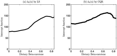
Figure 1: Plot of estimated intercept function of dietary beta-carotene: (a) the estimated intercept function by LS method; (b) the estimated intercept function by CQR method with $q=7$.

From Table 5, it can be seen that the CQR model is much sparser than the LS model. Only two covariates, “fiber consumption per day” and “fairly often use of vitamin” are included in the parametric part of the CQR model. Meanwhile, the CQR model has much better prediction performance than the LS model, whose MAPE is $111.28$.

6 Discussion

We discuss some directions in which this work could be further extended. We have focused on using uniform weights in composite quantile regression. In theory, we can use nonuniform weights, which may provide an even more efficient estimator when a reliable estimate of the error distribution is available. Koenker Koenker1984 discussed the theoretically optimal weights. Bradic, Fan and Wang Fan2010 suggested a data-driven weighted CQR for parametric linear regression, in which the weights mimic the optimal weights. The idea in Bradic, Fan and Wang Fan2010 can be easily extended to the semi-CQR estimator, which will be investigated in detail in a future paper.

Penalized Wilcoxon rank regression has been considered independently in Leng Leng10 and Wang and Li WangLi2009 and found to achieve a similar efficiency property of CQR for variable selection in parametric linear regression. We could also generalize rank regression to handle semiparametric varying-coefficient partially linear models. In a working paper, we show that rank regression is exactly equivalent to CQR using $q=n-1$ quantiles with uniform weights. This result indicates that CQR is more flexible than rank regression because we can easily use flexible nonuniform weights in CQR to further improve efficiency, as in Bradic, Fan and Wang Fan2010 . Obviously, CQR is also computationally more efficient than rank regression. We note that in parametric linear regression models, rank regression has no efficiency gain over least-squares for estimating the intercept. This result is expected to hold for estimating the baseline function in the semiparametric varying-coefficient partially linear model.

When the number of varying coefficient components is large, it is also desirable to consider selecting a few important components. This problem was studied in Wang and Xia WangXia09 , where a LASSO-type penalized local least-squares estimator was proposed. It would be interesting to apply CQR to their method to further improve the estimation efficiency.

7 Proofs

To establish the asymptotic properties of the proposed estimators, the following regularity conditions are imposed:

the random variable $U$ has bounded support $\Omega$ and its density function $f_{U}(\cdot)$ is positive and has a continuous second derivative;

the varying coefficients $\alpha_{0}(\cdot)$ and ${\bolds{\alpha}}(\cdot)$ have continuous second derivatives in $u\in\Omega$;

$K(\cdot)$ is a symmetric density function with bounded support and satisfies a Lipschitz condition;

the random vector $\mathbf{Z}$ has bounded support;

for the semi-QR procedure, [(C4)]

$F_{\tau}(0|u,\mathbf{x},\mathbf{z})=\tau$ for all $(u,\mathbf{x},\mathbf{z}),$ and $f_{\tau}(\cdot|u,\mathbf{x},\mathbf{z})$ is bounded away from zero and has a continuous and uniformly bounded derivative;

$\mathbf{A}_{1}(u)$ defined in Theorem 2.1 and $\mathbf{A}_{2}(u)$ defined in Theorem 2.3 are nonsingular for all $u\in\Omega$;

for the semi-CQR procedure, [(C4)]

$f(\cdot)$ is bounded away from zero and has a continuous and uniformly bounded derivative;

$\mathbf{D}_{1}(u)$ defined in Theorem 3.1 and $\mathbf{D}_{2}(u)$ defined in Theorem 3.3 are nonsingular for all $u\in\Omega$.

Although the proposed semi-QR and semi-CQR procedures require different regularity conditions, the proofs follow similar strategies. For brevity, we only present the detailed proofs for the semi-CQR procedure. The detailed proofs for the semi-QR procedure was given in the earlier version of this paper. Lemma 7.1 below, which is a direct result of Mack and Silverman MarkSilverman1982 , will be used repeatedly in our proofs. Throughout the proofs, identities of the form $G(u)=O_{p}(a_{n})$ always stand for $\sup_{u\in\Omega}|G(u)|=O_{p}(a_{n})$.

Lemma 7.1

Let $(\mathbf{X}_{1},Y_{1}),\ldots,(\mathbf{X}_{n},Y_{n})$ be i.i.d. random vectors, where the $Y_{i}$’s are scalar random variables. Assume, further, that $E|Y|^{r}<\infty$ and that $\sup_{\mathbf{x}}\int|y|^{r}f(\mathbf{x},y)\,dy<\infty$, where $f$ denotes the joint density of $(\mathbf{X},Y)$. Let $K$ be a bounded positive function with bounded support, satisfying a Lipschitz condition. Then,

$$\sup_{\mathbf{x}\in D}\Biggl{|}n^{-1}\sum_{i=1}^{n}\{K_{h}(\mathbf{X}_{i}-\mathbf{x})Y_{i}-E[K_{h}(\mathbf{X}_{i}-\mathbf{x})Y_{i}]\}\Biggr{|}=O_{p}\biggl{(}\frac{\log^{1/2}(1/h)}{\sqrt{nh}}\biggr{)},$$

provided that $n^{2\varepsilon-1}h\rightarrow\infty$ for some $\varepsilon<1-r^{-1}$.

Let $\eta_{i,k}=I(\varepsilon_{i}\leq c_{k})-\tau_{k}$ and $\eta^{*}_{i,k}(u)=I\{\varepsilon_{i}\leq c_{k}-r_{i}(u)\}-\tau_{k}$, where $r_{i}(u)=\alpha_{0}(U_{i})-\alpha_{0}(u)-\alpha^{\prime}_{0}(u)(U_{i}-u)+\mathbf{X}_{i}^{T}\{{\bolds{\alpha}}(U_{i})-{\bolds{\alpha}}(u)-{\bolds{\alpha}}^{\prime}(u)(U_{i}-u)\}$. Furthermore, let $\tilde{\bolds{\theta}}{}^{*}=\sqrt{nh}\{\tilde{a}_{01}-\alpha_{0}(u)-c_{1},\ldots,\tilde{a}_{0q}-\alpha_{0}(u)-c_{q},\{\tilde{\mathbf{a}}-{\bolds{\alpha}}(u)\}^{T},\{\tilde{\bolds{\beta}}-{\bolds{\beta}}_{0}\}^{T},h\{\tilde{b}_{0}-\alpha^{\prime}_{0}(u)\},h\{\tilde{\mathbf{b}}-{\bolds{\alpha}}^{\prime}(u)\}^{T}\}^{T}$ and $\mathbf{X}^{*}_{i,k}(u)=\{\mathbf{e}_{k}^{T},\mathbf{X}_{i}^{T},\break\mathbf{Z}_{i}^{T},(U_{i}-u)/h,\mathbf{X}_{i}^{T}(U_{i}-u)/h\}^{T}$, where $\mathbf{e}_{k}$ is a $q$-vector with 1 at the $k$th position and 0 elsewhere.

In the proof of Theorem 3.1, we will first show the following asymptotic representation of $\{\tilde{\mathbf{a}}_{0},\tilde{b}_{0},\tilde{\mathbf{a}},\tilde{\mathbf{b}},\tilde{\bolds{\beta}}\}$:

$$\tilde{\bolds{\theta}}{}^{*}=-f^{-1}_{U}(u)\{\mathbf{S}^{*}(u)\}^{-1}\mathbf{W}^{*}_{n}(u)+O_{p}\bigl{(}h^{2}+\log^{1/2}(1/h)/\sqrt{nh}\bigr{)},$$ (20)

where $\mathbf{S}^{*}(u)=\mathrm{diag}\{\mathbf{D}_{1}(u),c\mu_{2}\mathbf{B}_{2}(u)\}$ and

$$\mathbf{W}^{*}_{n}(u)=\frac{1}{\sqrt{nh}}\sum_{k=1}^{q}\sum_{i=1}^{n}K\{(U_{i}-u)/h\}\eta^{*}_{i,k}(u)\mathbf{X}_{i,k}^{*}(u).$$

The asymptotic normality of $\{\tilde{\mathbf{a}}_{0},\tilde{b}_{0},\tilde{\mathbf{a}},\tilde{\mathbf{b}},\tilde{\bolds{\beta}}\}$ then follows by demonstrating the asymptotic normality of $\mathbf{W}^{*}_{n}(u)$.

Proof of Theorem 3.1 Recall that $\{\tilde{\mathbf{a}}_{0},\tilde{\mathbf{a}},\tilde{\bolds{\beta}},\tilde{b}_{0},\tilde{\mathbf{b}}\}$ minimizes

$$\sum_{k=1}^{q}\sum_{i=1}^{n}\rho_{\tau_{k}}[Y_{i}-a_{0k}-b_{0}(U_{i}-u)-\mathbf{X}_{i}^{T}\{\mathbf{a}+\mathbf{b}(U_{i}-u)\}-\mathbf{Z}_{i}^{T}{\bolds{\beta}}]K_{h}(U_{i}-u).$$

We write $Y_{i}-a_{0k}-b_{0}(U_{i}-u)-\mathbf{X}_{i}^{T}\{\mathbf{a}+\mathbf{b}(U_{i}-u)\}-\mathbf{Z}_{i}^{T}{\bolds{\beta}}=(\varepsilon_{i}-c_{k})+r_{i}(u)-\Delta_{i,k}$, where $\Delta_{i,k}=\{\mathbf{X}_{i,k}^{*}(u)\}^{T}{\bolds{\theta}}^{*}/\sqrt{nh}$. Then, $\tilde{\bolds{\theta}}{}^{*}$ is also the minimizer of

$$L^{*}_{n}({\bolds{\theta}}^{*})=\sum_{k=1}^{q}\sum_{i=1}^{n}K_{i}(u)[\rho_{\tau_{k}}\{(\varepsilon_{i}-c_{k})+r_{i}(u)-\Delta_{i,k}\}-\rho_{\tau_{k}}\{(\varepsilon_{i}-c_{k})+r_{i}(u)\}],$$

where $K_{i}(u)=K\{(U_{i}-u)/h\}$. By applying the identity Knight1998

$$\qquad\rho_{\tau}(x-y)-\rho_{\tau}(x)=y\{I(x\leq 0)-\tau\}+\int_{0}^{y}\{I(x\leq z)-I(x\leq 0)\}\,dz,\vspace*{-1pt}$$ (21)

we have

$$L^{*}_{n}({\bolds{\theta}}^{*}) = \sum_{k=1}^{q}\sum_{i=1}^{n}K_{i}(u)\biggl{\{}\Delta_{i,k}[I\{\varepsilon_{i}\leq c_{k}-r_{i}(u)\}-\tau_{k}]\vspace*{-1pt}$$

$$\hphantom{\sum_{k=1}^{q}\sum_{i=1}^{n}K_{i}(u)\ }{}+\int_{0}^{\Delta_{i,k}}[I\{\varepsilon_{i}\leq c_{k}-r_{i}(u)+z\}-I\{\varepsilon_{i}\leq c_{k}-r_{i}(u)\}]\,dz\biggr{\}}$$

$$= \{\mathbf{W}^{*}_{n}(u)\}^{T}{\bolds{\theta}}^{*}+\sum_{k=1}^{q}B^{*}_{n,k}({\bolds{\theta}}^{*}),\vspace*{-1pt}$$

where

$$B^{*}_{n,k}({\bolds{\theta}}^{*})=\sum_{i=1}^{n}K_{i}(u)\int_{0}^{\Delta_{i,k}}[I\{\varepsilon_{i}\leq c_{k}-r_{i}(u)+z\}-I\{\varepsilon_{i}\leq c_{k}-r_{i}(u)\}]\,dz.\vspace*{-1pt}$$

Since $B^{*}_{n,k}({\bolds{\theta}}^{*})$ is a summation of i.i.d. random variables of the kernel form, it follows, by Lemma 7.1, that

$$B^{*}_{n,k}({\bolds{\theta}}^{*})=E[B^{*}_{n,k}({\bolds{\theta}}^{*})]+O_{p}\bigl{(}\log^{1/2}(1/h)/\sqrt{nh}\bigr{)}.\vspace*{-1pt}$$

The conditional expectation of $\sum_{k=1}^{q}B^{*}_{n,k}({\bolds{\theta}}^{*})$ can be calculated as

$$\sum_{k=1}^{q}E[B^{*}_{n,k}({\bolds{\theta}}^{*})|U,\mathbf{X},\mathbf{Z}]\vspace*{-1pt}$$

$$\qquad=\sum_{k=1}^{q}\sum_{i=1}^{n}K_{i}(u)\int_{0}^{\Delta_{i,k}}\bigl{[}F\bigl{(}c_{k}-r_{i}(u)+z\bigr{)}-F\bigl{(}c_{k}-r_{i}(u)\bigr{)}\bigr{]}\,dz$$

$$\qquad=\frac{1}{2}({\bolds{\theta}}^{*})^{T}\Biggl{(}\frac{1}{nh}\sum_{k=1}^{q}\sum_{i=1}^{n}K_{i}(u)f\bigl{(}c_{k}-r_{i}(u)\bigr{)}\{\mathbf{X}_{i,k}^{*}(u)\}\{\mathbf{X}_{i,k}^{*}(u)\}^{T}\Biggr{)}{\bolds{\theta}}^{*}$$

$$\qquad\quad{}+O_{p}\bigl{(}\log^{1/2}(1/h)/\sqrt{nh}\bigr{)}$$

$$\qquad\triangleq\frac{1}{2}({\bolds{\theta}}^{*})^{T}\mathbf{S}^{*}_{n}(u){\bolds{\theta}}^{*}+O_{p}\bigl{(}\log^{1/2}(1/h)/\sqrt{nh}\bigr{)}.\vspace*{-1pt}$$

Then,

$$L^{*}_{n}({\bolds{\theta}}^{*}) = \{\mathbf{W}^{*}_{n}(u)\}^{T}{\bolds{\theta}}^{*}+\sum_{k=1}^{q}E[B^{*}_{n,k}({\bolds{\theta}}^{*})]+O_{p}\bigl{(}\log^{1/2}(1/h)/\sqrt{nh}\bigr{)}$$

$$= \{\mathbf{W}^{*}_{n}(u)\}^{T}{\bolds{\theta}}^{*}+\sum_{k=1}^{q}E\{E[B^{*}_{n,k}({\bolds{\theta}}^{*})|U,\mathbf{X},\mathbf{Z}]\}+O_{p}\bigl{(}\log^{1/2}(1/h)/\sqrt{nh}\bigr{)}$$

$$= \{\mathbf{W}^{*}_{n}(u)\}^{T}{\bolds{\theta}}^{*}+\frac{1}{2}({\bolds{\theta}}^{*})^{T}E[\mathbf{S}^{*}_{n}(u)]{\bolds{\theta}}^{*}+O_{p}\bigl{(}\log^{1/2}(1/h)/\sqrt{nh}\bigr{)}.$$

It can be shown that $E[\mathbf{S}^{*}_{n}(u)]=f_{U}(u)\mathbf{S}^{*}(u)+O(h^{2})$. Therefore, we can write $L_{n}({\bolds{\theta}}^{*})$ as

$$L^{*}_{n}({\bolds{\theta}}^{*})=\{\mathbf{W}^{*}_{n}(u)\}^{T}{\bolds{\theta}}^{*}+\frac{f_{U}(u)}{2}({\bolds{\theta}}^{*})^{T}\mathbf{S}^{*}(u){\bolds{\theta}}^{*}+O_{p}\bigl{(}h^{2}+\log^{1/2}(1/h)/\sqrt{nh}\bigr{)}.$$

By applying the convexity lemma Pollard1991 and the quadratic approximation lemma FanGijbels1996 , the minimizer of $L^{*}_{n}({\bolds{\theta}}^{*})$ can be expressed as

$$\tilde{\bolds{\theta}}{}^{*}=-f^{-1}_{U}(u)\{\mathbf{S}^{*}(u)\}^{-1}\mathbf{W}^{*}_{n}(u)+O_{p}\bigl{(}h^{2}+\log^{1/2}(1/h)/\sqrt{nh}\bigr{)},$$ (22)

which holds uniformly for $u\in\Omega$. Meanwhile, for any point $u\in\Omega$, we have

$$\tilde{\bolds{\theta}}{}^{*}=-f^{-1}_{U}(u)\{\mathbf{S}^{*}(u)\}^{-1}\mathbf{W}^{*}_{n}(u)+o_{p}(1).$$ (23)

Note that $\mathbf{S}^{*}(u)=\mathrm{diag}\{\mathbf{D}_{1}(u),c\mu_{2}\mathbf{B}_{2}(u)\}$ is a quasi-diagonal matrix. So,

$$\sqrt{nh}\pmatrix{\tilde{\mathbf{a}}_{0}-{\bolds{\alpha}}_{0}(u)\vspace*{2pt}\cr\tilde{\mathbf{a}}-{\bolds{\alpha}}(u)\vspace*{2pt}\cr\tilde{\bolds{\beta}}-{\bolds{\beta}}_{0}}=-f^{-1}_{U}(u)\mathbf{D}^{-1}_{1}(u)\mathbf{W}^{*}_{n,1}(u)+o_{p}(1),$$ (24)

where $\mathbf{W}^{*}_{n,1}(u)=\frac{1}{\sqrt{nh}}\sum_{k=1}^{q}\sum_{i=1}^{n}K_{i}(u)\eta^{*}_{i,k}(u)(\mathbf{e}_{k}^{T},\mathbf{X}_{i}^{T},\mathbf{Z}_{i}^{T})^{T}$. Let

$$\mathbf{W}^{\#}_{n,1}(u)=\frac{1}{\sqrt{nh}}\sum_{k=1}^{q}\sum_{i=1}^{n}K_{i}(u)\eta_{i,k}(\mathbf{e}_{k}^{T},\mathbf{X}_{i}^{T},\mathbf{Z}_{i}^{T})^{T}.$$

Note that

$$\operatorname{Cov}({\eta}_{i,k},{\eta}_{i,k^{\prime}})={\tau}_{kk^{\prime}},\qquad\operatorname{Cov}({\eta}_{i,k},\eta_{j,k^{\prime}})=0\qquad\mbox{if }i\neq j.$$

By some calculations, we have that $E[\mathbf{W}^{\#}_{n,1}(u)]=\mathbf{0}$ and $\operatorname{Var}[\mathbf{W}^{\#}_{n,1}(u)]\rightarrow f_{U}(u)\nu_{0}{\bolds{\Sigma}}_{1}(u)$. By the Cramér–Wold theorem, the central limit theorem for $\mathbf{W}_{n,1}(u)$ holds. Therefore,

$$\mathbf{W}^{\#}_{n,1}(u)\stackrel{{\scriptstyle\mathcal{D}}}{{\longrightarrow}}N(\mathbf{0},f_{U}(u)\nu_{0}{\bolds{\Sigma}}_{1}(u)).$$

Moreover, we have $\operatorname{Var}[\mathbf{W}^{*}_{n,1}(u)-\mathbf{W}^{\#}_{n,1}(u)|U,\mathbf{X},\mathbf{Z}]\leq\frac{q^{2}}{nh}\sum_{i=1}^{n}K^{2}_{i}(u)(\mathbf{e}_{k}^{T},\mathbf{X}_{i}^{T},\break\mathbf{Z}_{i}^{T})^{T}(\mathbf{e}_{k}^{T},\mathbf{X}_{i}^{T},\mathbf{Z}_{i}^{T})\max_{k}\{F(c_{k}+|r_{i}|)-F(c_{k})\}=o_{p}(1)$, thus

$$\operatorname{Var}[\mathbf{W}^{*}_{n,1}(u)-\mathbf{W}^{\#}_{n,1}(u)]=o(1).$$

So, by Slutsky’s theorem, conditioning on $\{U,\mathbf{X},\mathbf{Z}\}$, we have

$$\mathbf{W}^{*}_{n,1}(u)-E[\mathbf{W}^{*}_{n,1}(u)]\stackrel{{\scriptstyle\mathcal{D}}}{{\longrightarrow}}N(\mathbf{0},f_{U}(u)\nu_{0}{\bolds{\Sigma}}_{1}(u)).$$ (25)

We now calculate the conditional mean of $\mathbf{W}^{*}_{n,1}(u)$:

$$\frac{1}{\sqrt{nh}}E[\mathbf{W}^{*}_{n,1}(u)|U,\mathbf{X},\mathbf{Z}]$$

$$\qquad=\frac{1}{nh}\sum_{k=1}^{q}\sum_{i=1}^{n}K_{i}(u)\bigl{\{}F\bigl{(}c_{k}-r_{i}(u)\bigr{)}-F(c_{k})\bigr{\}}(\mathbf{e}_{k}^{t},\mathbf{X}_{i}^{T},\mathbf{Z}_{i}^{T})^{T}$$

(26)

$$\qquad=-\frac{1}{nh}\sum_{k=1}^{q}\sum_{i=1}^{n}K_{i}(u)r_{i}(u)f(c_{k})\{1+o(1)\}(\mathbf{e}_{k}^{t},\mathbf{X}_{i}^{T},\mathbf{Z}_{i}^{T})^{T}$$

$$\qquad=-\frac{\mu_{2}h^{2}}{2}f_{U}(u)\mathbf{D}_{1}(u)\pmatrix{{\bolds{\alpha}}^{\prime\prime}_{0}(u)\vspace*{3pt}\cr{\bolds{\alpha}}^{\prime\prime}(u)\vspace*{2pt}\cr\mathbf{0}}+o_{p}(h^{2}).$$

The proof is completed by combining (24), (25) and (7).

Proof of Theorem 3.2 Let ${\bolds{\theta}}=\sqrt{n}({\bolds{\beta}}-{\bolds{\beta}}_{0})$. Then,

$$Y_{i}-\tilde{a}_{0k}(U_{i})-\mathbf{X}_{i}^{T}\tilde{\mathbf{a}}(U_{i})-\mathbf{Z}_{i}^{T}{\bolds{\beta}}$$

$$\qquad=\varepsilon_{i}-c_{k}-\{\tilde{a}_{0k}(U_{i})-\alpha_{0}(U_{i})-c_{k}\}-\mathbf{X}_{i}^{T}\{\tilde{\mathbf{a}}(U_{i})-{\bolds{\alpha}}(U_{i})\}-\mathbf{Z}_{i}^{T}({\bolds{\beta}}-{\bolds{\beta}}_{0})$$

$$\qquad=\varepsilon_{i}-c_{k}-\tilde{r}_{i,k}-\mathbf{Z}_{i}^{T}{\bolds{\theta}}/\sqrt{n},$$

where $\tilde{r}_{i,k}=\{\tilde{a}_{0k}(U_{i})-\alpha_{0}(U_{i})-c_{k}\}+\mathbf{X}_{i}^{T}\{\tilde{\mathbf{a}}(U_{i})-{\bolds{\alpha}}(U_{i})\}$. Then,

$$\hat{\bolds{\theta}}=\operatorname{argmin}\sum_{k=1}^{q}\sum_{i=1}^{n}\rho_{\tau_{k}}\bigl{(}Y_{i}-\tilde{a}_{0k}(U_{i})-\mathbf{X}_{i}^{T}\tilde{\mathbf{a}}(U_{i})-\mathbf{Z}_{i}^{T}{\bolds{\beta}}\bigr{)}$$

is also the minimizer of

$$L_{n}({\bolds{\theta}})=\sum_{k=1}^{q}\sum_{i=1}^{n}\bigl{\{}\rho_{\tau_{k}}\bigl{(}\varepsilon_{i}-c_{k}-\tilde{r}_{i,k}-\mathbf{Z}_{i}^{T}{\bolds{\theta}}/\sqrt{n}\bigr{)}-\rho_{\tau_{k}}(\varepsilon_{i}-c_{k}-\tilde{r}_{i,k})\bigr{\}}.$$

By applying the identity (21), we can rewrite $L_{n}({\bolds{\theta}})$ as follows:

$$L_{n}({\bolds{\theta}}) = \sum_{k=1}^{q}\sum_{i=1}^{n}\biggl{\{}\frac{\mathbf{Z}_{i}^{T}{\bolds{\theta}}}{\sqrt{n}}[I(\varepsilon_{i}\leq c_{k})-\tau_{k}]$$

$$\hphantom{\sum_{k=1}^{q}\sum_{i=1}^{n}\biggl{\{}}{}+\int_{\tilde{r}_{i,k}}^{\tilde{r}_{i,k}+\mathbf{Z}_{i}^{T}{\bolds{\theta}}/\sqrt{n}}[I(\varepsilon_{i}\leq c_{k}+z)-I(\varepsilon_{i}\leq c_{k})]\,dz\biggr{\}}$$

$$= \Biggl{(}\frac{1}{\sqrt{n}}\sum_{k=1}^{q}\sum_{i=1}^{n}\eta_{i,k}\mathbf{Z}_{i}\Biggr{)}^{T}{\bolds{\theta}}+B_{n}({\bolds{\theta}}),$$

where $B_{n}({\bolds{\theta}})=\sum_{k=1}^{q}\sum_{i=1}^{n}\int_{\tilde{r}_{i,k}}^{\tilde{r}_{i,k}+\mathbf{Z}_{i}^{T}{\bolds{\theta}}/\sqrt{n}}[I(\varepsilon_{i}\leq c_{k}+z)-I(\varepsilon_{i}\leq c_{k})]\,dz$. Let us now calculate the conditional expectation of $B_{n}({\bolds{\theta}})$:

$$E[B_{n}({\bolds{\theta}})|U,\mathbf{X},\mathbf{Z}]$$

$$\qquad=\sum_{k=1}^{q}\sum_{i=1}^{n}\int_{\tilde{r}_{i,k}}^{\tilde{r}_{i,k}+\mathbf{Z}_{i}^{T}{\bolds{\theta}}/\sqrt{n}}[zf(c_{k})\{1+o(1)\}]\,dz$$

$$\qquad=\frac{1}{2}{\bolds{\theta}}^{T}\Biggl{(}\frac{1}{n}\sum_{k=1}^{q}\sum_{i=1}^{n}f(c_{k})\mathbf{Z}_{i}\mathbf{Z}_{i}^{T}\Biggr{)}{\bolds{\theta}}-\Biggl{(}\frac{1}{\sqrt{n}}\sum_{k=1}^{q}\sum_{i=1}^{n}f(c_{k})\tilde{r}_{i,k}\mathbf{Z}_{i}\Biggr{)}^{T}{\bolds{\theta}}+o_{p}(1).$$

Define $R_{n}({\bolds{\theta}})=B_{n}({\bolds{\theta}})-E[B_{n}({\bolds{\theta}})|U,\mathbf{X},\mathbf{Z}]$. It can be shown that $R_{n}({\bolds{\theta}})=o_{p}(1)$. Hence,

$$L_{n}({\bolds{\theta}}) = \Biggl{(}\frac{1}{\sqrt{n}}\sum_{k=1}^{q}\sum_{i=1}^{n}\eta_{i,k}\mathbf{Z}_{i}\Biggr{)}^{T}{\bolds{\theta}}+E[B_{n}({\bolds{\theta}})|U,\mathbf{X},\mathbf{Z}]+R_{n}({\bolds{\theta}})$$

$$= \frac{1}{2}{\bolds{\theta}}^{T}\mathbf{S}_{n}{\bolds{\theta}}+\Biggl{(}\frac{1}{\sqrt{n}}\sum_{k=1}^{q}\sum_{i=1}^{n}\eta_{i,k}\mathbf{Z}_{i}\Biggr{)}^{T}{\bolds{\theta}}-\Biggl{(}\frac{1}{\sqrt{n}}\sum_{k=1}^{q}\sum_{i=1}^{n}f(c_{k})\tilde{r}_{i,k}\mathbf{Z}_{i}\Biggr{)}^{T}{\bolds{\theta}}$$

$${}+o_{p}(1),$$

where $\mathbf{S}_{n}=\frac{1}{n}\sum_{k=1}^{q}\sum_{i=1}^{n}f(c_{k})\mathbf{Z}_{i}\mathbf{Z}_{i}^{T}$. By (22), the third term in the previous expression can be expressed as

$$\frac{1}{\sqrt{n}}\sum_{k=1}^{q}\sum_{i=1}^{n}f(c_{k})\tilde{r}_{i,k}\mathbf{Z}_{i}$$

$$\qquad=\frac{1}{\sqrt{n}}\sum_{k=1}^{q}\sum_{i=1}^{n}\frac{f(c_{k})}{f_{U}(U_{i})}\mathbf{Z}_{i}\pmatrix{\mathbf{e}_{k}\vspace*{2pt}\cr\mathbf{X}_{i}\vspace*{2pt}\cr\mathbf{0}}^{T}$$

$$\qquad\hphantom{=\frac{1}{\sqrt{n}}\sum_{k=1}^{q}\sum_{i=1}^{n}}{}\times\mathbf{D}_{1}^{-1}(U_{i})\left(\frac{1}{nh}\sum_{k^{\prime}=1}^{q}\sum_{i^{\prime}=1}^{n}\eta^{*}_{i^{\prime},k^{\prime}}(U_{i})\pmatrix{\mathbf{e}_{k^{\prime}}\vspace*{2pt}\cr\mathbf{X}_{i^{\prime}}\vspace*{2pt}\cr\mathbf{Z}_{i^{\prime}}}K_{i^{\prime}}(U_{i})\right)$$

$$\qquad\quad{}+O_{p}\bigl{(}h^{3/2}+\log^{1/2}(1/h)/\sqrt{nh^{2}}\bigr{)}$$

$$\qquad=\frac{1}{\sqrt{n}}\sum_{k^{\prime}=1}^{q}\sum_{i^{\prime}=1}^{n}\eta_{i^{\prime},k^{\prime}}\bolds{\delta}_{k^{\prime}}(U_{i^{\prime}},\mathbf{X}_{i^{\prime}},\mathbf{Z}_{i^{\prime}})+O_{p}\bigl{(}n^{1/2}h^{2}+\log^{1/2}(1/h)/\sqrt{nh^{2}}\bigr{)}$$

$$\qquad=\frac{1}{\sqrt{n}}\sum_{k=1}^{q}\sum_{i=1}^{n}\eta_{i,k}\bolds{\delta}_{k}(U_{i},\mathbf{X}_{i},\mathbf{Z}_{i})+o_{p}(1),$$

where

$$\bolds{\delta}(U_{i},\mathbf{X}_{i},\mathbf{Z}_{i})=E[\mathbf{Z}(\mathbf{c}^{T},c\mathbf{X}^{T},\mathbf{0})|U=U_{i}]\mathbf{D}_{1}^{-1}(U_{i})(I_{q},\mathbf{1}^{T}\mathbf{X}_{i},\mathbf{1}^{T}\mathbf{Z}_{i})^{T}.$$

Therefore,

$$L_{n}({\bolds{\theta}}) = \frac{1}{2}{\bolds{\theta}}^{T}\mathbf{S}_{n}{\bolds{\theta}}+\Biggl{(}\frac{1}{\sqrt{n}}\sum_{k=1}^{q}\sum_{i=1}^{n}\eta_{i,k}\{\mathbf{Z}_{i}-\bolds{\delta}_{k}(U_{i},\mathbf{X}_{i},\mathbf{Z}_{i})\}\Biggr{)}^{T}{\bolds{\theta}}+o_{p}(1)$$

$$\triangleq \frac{1}{2}{\bolds{\theta}}^{T}\mathbf{S}_{n}{\bolds{\theta}}+\mathbf{W}_{n}^{T}{\bolds{\theta}}+o_{p}(1).$$

It can be shown that $\mathbf{S}_{n}=E(\mathbf{S}_{n})+o_{p}(1)=c\mathbf{S}+o_{p}(1)$. Hence,

$$L_{n}({\bolds{\theta}})=\frac{c}{2}{\bolds{\theta}}^{T}\mathbf{S}{\bolds{\theta}}+\mathbf{W}_{n}^{T}{\bolds{\theta}}+o_{p}(1).$$

Since the convex function $L_{n}({\bolds{\theta}})-\mathbf{W}_{n}^{T}{\bolds{\theta}}$ converges in probability to the convex function $\frac{c}{2}{\bolds{\theta}}^{T}\mathbf{S}{\bolds{\theta}}$, it follows, by the convexity lemma Pollard1991 , that the quadratic approximation to $L_{n}({\bolds{\theta}})$ holds uniformly for ${\bolds{\theta}}$ in any compact set $\Theta$. Thus, it follows that

$$\hat{{\bolds{\theta}}}=-\frac{1}{c}\mathbf{S}^{-1}\mathbf{W}_{n}+o_{p}(1).$$ (27)

By the Cramér–Wold theorem, the central limit theorem for $\mathbf{W}_{n}$ holds and $\operatorname{Var}(\mathbf{W}_{n})\rightarrow{\bolds{\Delta}}=\sum_{k=1}^{q}\sum_{k^{\prime}=1}^{q}\tau_{kk^{\prime}}E\{\mathbf{Z}-\bolds{\delta}_{k}(U,\mathbf{X},\mathbf{Z})\}\{\mathbf{Z}-\bolds{\delta}_{k^{\prime}}(U,\mathbf{X},\mathbf{Z})\}^{T}$. Therefore, the asymptotic normality of $\hat{\bolds{\beta}}$ is followed by

$$\sqrt{n}(\hat{\bolds{\beta}}-{\bolds{\beta}}_{0})\stackrel{{\scriptstyle\mathcal{D}}}{{\longrightarrow}}N\biggl{(}0,\frac{1}{c^{2}}\mathbf{S}^{-1}{\bolds{\Delta}}\mathbf{S}^{-1}\biggr{)}.$$

This completes the proof.

Proof of Theorem 3.3 The asymptotic normality of $\hat{\alpha}_{0}(u)$ and $\hat{\bolds{\alpha}}(u)$ can be obtained by following the ideas in the proof of Theorem 3.1.

Proof of Theorem 4.1 Use the same notation as in the proof of Theorem 3.2. Minimizing

$$\sum_{k=1}^{q}\sum_{i=1}^{n}\rho_{\tau_{k}}\{Y_{i}-\tilde{a}_{0k}(U_{i})-\mathbf{X}_{i}^{T}\tilde{\mathbf{a}}(U_{i})-\mathbf{Z}_{i}^{T}{\bolds{\beta}}\}+nq\sum_{j=1}^{d}p^{\prime}_{\lambda_{j}}\bigl{(}\bigl{|}\beta_{j}^{(0)}\bigr{|}\bigr{)}|\beta_{j}|$$

is equivalent to minimizing

$$G_{n}({\bolds{\theta}}) = \sum_{k=1}^{q}\sum_{i=1}^{n}\bigl{\{}\rho_{\tau_{k}}\bigl{(}\varepsilon_{i}-c_{k}-\tilde{r}_{i,k}-\mathbf{Z}_{i}^{T}{\bolds{\theta}}/\sqrt{n}\bigr{)}-\rho_{\tau_{k}}(\varepsilon_{i}-c_{k}-\tilde{r}_{i,k})\bigr{\}}$$

$${}+nq\sum_{j=1}^{d}p^{\prime}_{\lambda_{j}}\bigl{(}\bigl{|}\beta_{j}^{(0)}\bigr{|}\bigr{)}(|\beta_{j}|-|\beta_{0j}|)$$

$$= \frac{c}{2}{\bolds{\theta}}^{T}\mathbf{S}{\bolds{\theta}}+\mathbf{W}_{n}^{T}{\bolds{\theta}}+nq\sum_{j=1}^{d}p^{\prime}_{\lambda_{j}}\bigl{(}\bigl{|}\beta_{j}^{(0)}\bigr{|}\bigr{)}(|\beta_{j}|-|\beta_{0j}|)+o_{p}(1),$$

where ${\bolds{\theta}}=\sqrt{n}({\bolds{\beta}}-{\bolds{\beta}}_{0})$ and $\tilde{r}_{i,k}=\{\tilde{a}_{0k}(U_{i})-\alpha_{0}(U_{i})-c_{k}\}+\mathbf{X}_{i}^{T}\{\tilde{\mathbf{a}}(U_{i})-{\bolds{\alpha}}(U_{i})\}$. Similar to the derivation in the proof of Theorem 5 in Zou and Li ZouLi2008 , the third term above can be expressed as

$$nq\sum_{j=1}^{d}p^{\prime}_{\lambda_{j}}\bigl{(}\bigl{|}\beta_{j}^{(0)}\bigr{|}\bigr{)}(|\beta_{j}|-|\beta_{0j}|)\stackrel{{\scriptstyle\mathcal{P}}}{{\longrightarrow}}\cases{0,&\quad if ${\bolds{\beta}}_{2}={\bolds{\beta}}_{20}$,\cr\infty,&\quad otherwise.}$$ (28)

Therefore, by the epiconvergence results Geyer1994 , KnightFu2000 , we have $\hat{\bolds{\beta}}{}^{\mathrm{OSE}}_{2}\stackrel{{\scriptstyle\mathcal{P}}}{{\longrightarrow}}0$ and the asymptotic results for $\hat{\bolds{\beta}}{}^{\mathrm{OSE}}_{1}$ holds.

To prove sparsity, we only need to show that $\hat{\bolds{\beta}}{}^{\mathrm{OSE}}_{2}=0$ with probability tending to 1. It suffices to prove that if $\beta_{0j}=0$, then $P(\hat{\beta}_{j}^{\mathrm{OSE}}\neq 0)\rightarrow 0$. By using the fact that $|\frac{\rho_{\tau}(t_{1})-\rho_{\tau}(t_{2})}{t_{1}-t_{2}}|\leq\max(\tau,1-\tau)<1$, if $\hat{\beta}_{j}^{\mathrm{OSE}}\neq 0$, then we must have $\sqrt{n}p^{\prime}_{\lambda_{j}}(|\beta_{j}^{(0)}|)<\frac{1}{n}\sum_{i=1}^{n}|Z_{ij}|$. Thus, we have $P(\hat{\beta}_{j}^{\mathrm{OSE}}\neq 0)\leq P(\sqrt{n}p^{\prime}_{\lambda_{j}}(|\beta_{j}^{(0)}|)<\frac{1}{n}\sum_{i=1}^{n}|Z_{ij}|)$. However, under the assumptions, we have $\sqrt{n}p^{\prime}_{\lambda_{j}}(|\beta_{j}^{(0)}|)\rightarrow\infty$. Therefore, $P(\hat{\beta}_{j}^{\mathrm{OSE}}\neq 0)\rightarrow 0$. This completes the proof.

References

• (1) Bradic, J., Fan, J. and Wang, W. (2010). Penalized composite quasi-likelihood for ultrahigh-dimensional variable selection. Available at arXiv:0912.5200v1.
• (2) Cai, Z. and Xu, X. (2009). Nonparametric quantile estimations for dynamic smooth coefficient models. J. Amer. Statist. Assoc. 104 371–383. \MR2504383
• (3) Carroll, R., Fan, J., Gijbels, I. and Wand, M. (1997). Generalized partially linear single-index models. J. Amer. Statist. Assoc. 92 477–489. \MR1467842
• (4) Fan, J. and Gijbels, I. (1996). Local Polynomial Modelling and Its Applications. Chapman & Hall, London. \MR1383587
• (5) Fan, J. and Huang, T. (2005). Profile likelihood inferences on semiparametric varying-coefficient partially linear models. Bernoulli 11 1031–1057. \MR2189080
• (6) Fan, J. and Li, R. (2001). Variable selection via nonconcave penalized likelihood and its oracle properties. J. Amer. Statist. Assoc. 96 1348–1361. \MR1946581
• (7) Fan, J. and Li, R. (2006). Statistical challenges with high dimensionality: Feature selection in knowledge discovery. In Proceedings of the International Congress of Mathematicians (M. Sanz-Sole, J. Soria, J. Varona and J. Verdera, eds.) III 595–622. Eur. Math. Soc., Zürich. \MR2275698
• (8) Geyer, C. (1994). On the asymptotics of constrained M-estimation. Ann. Statist. 22 1993–2010. \MR1329179
• (9) Härdle, W., Liang, H. and Gao, J. (2000). Partially Linear Models. Physica Verlag, Heidelberg. \MR1787637
• (10) He, X. and Shi, P. (1996). Bivariate tensor-product B-splines in a partly linear model. J. Multivariate Anal. 58 162–181. \MR1405586
• (11) He, X., Zhu, Z. and Fung, W. (2002). Estimation in a semiparametric model for longitudinal data with unspecified dependence structure. Biometrika 89 579–590. \MR1929164
• (12) Hunter, D. and Li, R. (2005). Variable selection using MM algorithms. Ann. Statist. 33 1617–1642. \MR2166557
• (13) Kai, B., Li, R. and Zou, H. (2010). Local composite quantile regression smoothing: An efficient and safe alternative to local polynomial regression. J. Roy. Statist. Soc. Ser. B 72 49–69.
• (14) Knight, K. (1998). Limiting distributions for $L_{1}$ regression estimators under general conditions. Ann. Statist. 26 755–770. \MR1626024
• (15) Knight, K. and Fu, W. (2000). Asymptotics for lasso-type estimators. Ann. Statist. 28 1356–1378. \MR1805787
• (16) Koenker, R. (1984). A note on L-estimates for linear models. Statist. Probab. Lett. 2 323-325. \MR0782652
• (17) Koenker, R. (2005). Quantile Regression. Cambridge Univ. Press, Cambridge. \MR2268657
• (18) Lam, C. and Fan, J. (2008). Profile-kernel likelihood inference with diverging number of parameters. Ann. Statist. 36 2232–2260. \MR2458186
• (19) Lee, S. (2003). Efficient semiparametric estimation of a partially linear quantile regression model. Econometric Theory 19 1–31. \MR1965840
• (20) Leng, C. (2010). Variable selection and coefficient estimation via regularized rank regression. Statist. Sinica 20 167–181. \MR2640661
• (21) Li, R. and Liang, H. (2008). Variable selection in semiparametric regression modeling. Ann. Statist. 36 261–286. \MR2387971
• (22) Li, Y. and Zhu, J. (2007). $L_{1}$-norm quantile regression. J. Comput. Graph. Statist. 17 163–185. \MR2424800
• (23) Mack, Y. and Silverman, B. (1982). Weak and strong uniform consistency of kernel regression estimates. Probab. Theory Related Fields 61 405–415. \MR0679685
• (24) Nierenberg, D., Stukel, T., Baron, J., Dain, B. and Greenberg, E. (1989). Determinants of plasma levels of beta-carotene and retinol. American Journal of Epidemiology 130 511–521.
• (25) Pollard, D. (1991). Asymptotics for least absolute deviation regression estimators. Econometric Theory 7 186–199. \MR1128411
• (26) Ruppert, D., Wand, M. and Carroll, R. (2003). Semiparametric Regression. Cambridge Univ. Press, Cambridge. \MR1998720
• (27) Wang, H., Li, R. and Tsai, C. (2007). Tuning parameter selectors for the smoothly clipped absolute deviation method. Biometrika 94 553–568. \MR2410008
• (28) Wang, H. and Xia, Y. (2009). Shrinkage estimation of the varying coefficient model. J. Amer. Statist. Assoc. 104 747–757. \MR2541592
• (29) Wang, L. and Li, R. (2009). Weighted Wilcoxon-type smoothly clipped absolute deviation method. Biometrics 65 564–571.
• (30) Wu, Y. and Liu, Y. (2009). Variable selection in quantile regression. Statist. Sinica 19 801–817. \MR2514189
• (31) Xia, Y., Zhang, W. and Tong, H. (2004). Efficient estimation for semivarying-coefficient models. Biometrika 91 661–681. \MR2090629
• (32) Yatchew, A. (2003). Semiparametric Regression for the Applied Econometrician. Cambridge Univ. Press, Cambridge.
• (33) Zhang, W., Lee, S. and Song, X. (2002). Local polynomial fitting in semivarying coefficient model. J. Multivariate Anal. 82 166–188. \MR1918619
• (34) Zou, H. and Li, R. (2008). One-step sparse estimates in nonconcave penalized likelihood models (with discussion). Ann. Statist. 36 1509–1533. \MR2435443
• (35) Zou, H. and Yuan, M. (2008). Composite quantile regression and the oracle model selection theory. Ann. Statist. 36 1108–1126. \MR2418651