Abstract

From the analysis of Supernova Ia data alongwith Observational Hubble Data (OHD) and Baryon Acoustic Oscillation (BAO) data, we attempt to find out the nature of a scalar potential that may be responsible for the Dark Energy of the universe. We demonstrate that in order to explain the varying dark energy equation of state ($\omega_{X}(z)$) as obtained in a model independent way from the analyses of observational data , we need to invoke a quintom scalar field having a “quintessence” part for $\omega_{X}(z)>-1$ and a “phantom” part for $\omega_{X}(z)<-1$. We consider a Gaussian type potential for these scalar fields and compare the dark energy equation of state derived from such potential with the one computed from the data analysis.

1 Introduction

The recent acceleration of the expansion rate of the universe that has been inferred from the observation and luminosity distance measurements of different Supernova Ia (SNe Ia) [1] at different redshifts ($z$) is thought to be caused by the existence of a mysterious energy called dark energy. Different other observational evidence (such as WMAP [2], Cosmic Microwave Background (CMB) [3]) etc. suggest that this dark energy accounts for almost 73% of the content of the universe. Dark energy is a hypothetical energy component with a negative pressure responsible for causing the universe to experience this accelerated expansion. Although there are efforts to understand its nature and origin, dark energy still remains an enigma.

An attempt to explain dark energy involvs considering a slowly varying potential $V(\phi)$ of a scalar field $\phi$. Hence for such considerations the knowledge of $\phi$ and $V(\phi)$ are necessary in order to get an insight of dark energy and its equation of state. In FRW cosmology, it can be shown that in cosmological constant scenario , the dark energy equation of state remains constant at the value -1 all along the evolution history of the universe. However if dark energy varies with time or equivalently with redshift $z$, a possible explanation may be given by a scalar field (quintessence field) for dark energy equation of state $\omega(z)\geq-1$. But one needs to invoke a phantom scalar field $\sigma$ in case $\omega(z)$ falls below $-1$.

In the present work, we have considered five different SNe Ia data sets alongwith Observational Hubble Data (OHD) [4] and Baryon Acoustic Oscillation Data (BAO) [5]. The data sets are made available from Riess et al (2007)[6], Wood-Vasey et al (2007)[7], Davis et al[8], Kowalski et al (2008)[9], Kessler et al (2009) [10] and Amanullah et al (2010) (also known as Union2 data)[11]. The maximum span of redshift $z$ for these compilations for distance modulus $\mu(z)$ (related to the luminosity distance $d_{L}(z)$) are in the range $0.001\leq z\leq 1.76$. A parametric form for $d_{L}(z)$ is chosen whose parameters are obtained from a $\chi^{2}$ minimization of various observational data mentioned above. The dark energy equation of state can be derived analytically using an analytic form of $d_{L}(z)$, such as the present parametric form. With the fitted values of the parameters the dark energy equation of state $\omega_{X}(z)$ can therefore be calculated. On the otherhand, since $d_{L}(z)$ is related to the Hubble parameter $H(z)$ by an analytical expression one can use the same parametric form for $d_{L}(z)$ (with parameters from $\chi^{2}$ analyses) and evaluate both the quintessence scalar field $\phi$ and the phantom field $\sigma$ and their variations with the redshift $z$ (see later). With chosen form of potentials for both $\phi$ and $\sigma$, one can then compute the dark energy equation of state ($\omega(z)$) from the $\phi$ and $\sigma$ values obtained from the analysis. In this work, we have taken the form of this potential as $V=V(\phi)+V(\sigma)$, where $V(\phi)$ and $V(\sigma)$ are chosen to be $V(\phi)=V_{0}\exp[\lambda_{1}(1+(\phi(z)-\phi_{0})^{2}/M^{2}_{pl})]$ and $V(\sigma)=V_{0}\exp[\lambda_{2}(1+(\sigma(z)-\sigma_{0})^{2}/M^{2}_{pl})]$, where $\phi_{0}$($\sigma_{0}$) is the value of $\phi$($\sigma$) at present epoch and $M_{pl}$ is the Planck mass. We refer the dark energy equation of state computed from the scalar fields with this potential, as $\omega(z)$. The $\omega(z)$ thus obtained is then compared with the $\omega_{X}(z)$ computed directly from the analysis of $\mu_{L}(z)$ data with the assumption that the present universe is spatially flat and contains only matter and dark energy.

The paper is organised as follows. In Sect. 2 we discuss the dark energy equation of state as derived from FRW cosmology. In Sect. 3 we propose a quintom scalar formalism of dark energy. The calculational procedures are given in Sect. 4. Finally in Sect. 5 we furnish our calculational results and discussions.

2 Brief overview of model independent reconstruction of dark energy equation of state

For a homogeneous and isotropic universe the Friedmann-Robertson-Walker metric is given by

$$ds^{2} = -dt^{2}+a^{2}(t)\left[\frac{dr^{2}}{1-Kr^{2}}+r^{2}(d\theta^{2}+sin^{2}\theta d\phi^{2})\right]\,\,.$$ (1)

where $a(t)$ is the scale factor and $K$ is the curvature parameter. Considering the universe to be a perfect fluid characterized by energy density $\rho$ and pressure $p$, the Einstein’s equation alongwith Eq. (1) leads to two independent equations (for spatially flat universe),

$$H^{2}(t) = \frac{8\pi G}{3}\rho(t)$$ (2)

$$\dot{H}(t) = -4\pi G(p+\rho)$$ (3)

where $H(t)=\frac{1}{a(t)}\frac{d}{dt}(a(t))$ is the Hubble parameter that denotes the expansion rate of universe.

From Eq. (2) and Eq. (3) one gets

$$\frac{\ddot{a}(t)}{a(t)}=-\frac{4\pi G}{3}(\rho+3p)\,.$$ (4)

Assuming the universe contains only matter and dark energy, Eq. (2) leads to the result

$$\frac{H^{2}(z)}{H_{0}^{2}}=\Omega_{m}^{0}(1+z)^{3}+\Omega_{X}^{0}\exp\left(\int_{0}^{z}3(1+\omega_{X}(z))\frac{dz}{1+z}\right)\,\,,$$ (5)

where the symbol $\Omega$ represents energy density or matter density normalised to the critical density $\rho_{c}$ of the universe and thus $\Omega_{m}^{0}$ ($\Omega_{X}^{0}$) represents the matter (dark energy) density parameter at present epoch. As mentioned earlier in this section that universe contains only matter and dark energy in the redshift range considered here, we have $\Omega_{m}(z)+\Omega_{X}(z)=1$. From Eq. (5) the equation of state of dark energy $\omega_{X}(z)$ can be derived as,

$$\omega_{X}(z) = -1+\left[\frac{\frac{2}{3}\frac{(1+z)}{H(z)}\frac{dH(z)}{dz}-\Omega_{m}^{0}\frac{(1+z)^{3}}{H^{2}(z)}H_{0}^{2}}{1-\Omega_{m}^{0}\frac{(1+z)^{3}}{H^{2}(z)}H_{0}^{2}}\right]$$ (6)

The SNe Ia observational data are tabulated as a distance modulus $\mu(z)$. This is related to luminosity distance $d_{L}(z)$ by

$$\mu(z) = 5\log_{10}(d_{L}/Mpc)+25$$ (7)

for a redshift value $z$ at which the observation was made. The observed distance modulus $\mu_{\rm obs}(z)$ is related to the apparent magnitude $m_{\rm obs}(z)$ of a SNe Ia and absolute magnitude $M$ through the equation $\mu_{\rm obs}(z)=m_{\rm obs}(z)-M$. Also for spatially flat universe Hubble parameter and the luminosity distance are related through

$$H(z) = c\left[\frac{d}{dz}\left(\frac{d_{L}(z)}{(1+z)}\right)\right]^{-1}\,\,.$$ (8)

As stated in Sect. 1 a parametric form of $d_{L}(z)$ is considered and the parameters are obtained from a $\chi^{2}$ fit of the observational data. The dark energy equation of state $\omega_{X}(z)$ can then be reconstructed using the Eqns (1 - 5) and Eq. (6). We also mention here that a combined $\chi^{2}$ fit is made with SNe Ia data, OHD and BAO data.

3 Dark energy equation of state in a scalar field theory framework

The acceleration equation (Eq. (4)) suggests that the universe containing a perfect fluid can undergo accelerated expansion only if the pressure of the fluid is negative. A suitably chosen real scalar field can produce negative pressure in the FRW spacetime and may also lead to time varying equation of state of the perfect fluid depending on the potential of the field. Therefore such a real scalar field can be a possible candidate for time varying dark energy. The scalar fields naturally arise in particle physics theories including string theory. There exists in literature a wide variety of scalar field dark energy models. In this work we consider a quintom scalar field model where the two scalar fields namely $\phi(z)$ and $\sigma(z)$ are responsible for dark energy and the variation of its equation of state with redshift $z$. Each of the fields has specified form of potential and the two kinds of fields are not coupled to each other. We like to show that this simple model can explain the varying dark energy equation of state $\omega_{X}(z)$ obtained by using the combined $\chi^{2}$ analyses results of SNe data, OHD data, BAO data in Eq. (6).

3.1 Dark energy and quintessence scalar field

The action $S$ for Quintessence scalar field is given by (with $V(\phi)$, the potential of the field $\phi$),

$$S = S_{m}+\int d^{4}x\sqrt{-g}\left[\frac{1}{2}g^{\mu\nu}(\partial_{\mu}\phi)\partial_{\nu}\phi)+V(\phi)\right]\,\,,$$ (9)

where $S_{m}$ is the matter action. The equation of motion of the spatially homogeneous quintessence field is given by

$$\ddot{\phi}(t)+3H(t)\dot{\phi}(t)+\frac{dV(\phi)}{d\phi} = 0\,\,\,\,.$$ (10)

The Eq. (10) will lead to

$$\dot{\phi}^{2}(t)=-\frac{1}{8\pi GH(t)}\frac{d}{dt}(H_{\phi}^{2})\,\,\,\,,$$ (11)

where $H_{\phi}^{2}=\frac{8\pi G}{3}\left(\frac{1}{2}\dot{\phi}^{2}(t)+V(\phi)\right)$ and $H^{2}=\frac{8\pi G}{3}\left(\frac{1}{2}\dot{\phi}^{2}(t)+V(\phi)+\rho_{m}\right)$. The Energy momentum tensor for quintessence scalar field can be written as

$$T^{\mu}_{\nu} = g^{\mu\alpha}\partial_{\alpha}\phi\partial_{\nu}\phi-\delta^{\mu}_{\nu}\left(\frac{1}{2}g^{\alpha\beta}\partial_{\alpha}\phi\partial_{\beta}\phi+V(\phi)\right)$$ (12)

From Eq. (12) we have,

$$\rho_{\phi} = -T^{0}_{0}=\frac{1}{2}\dot{\phi}^{2}+V(\phi)$$ (13)

$$p_{\phi} = T^{i}_{i}=\frac{1}{2}\dot{\phi}^{2}-V(\phi)$$ (14)

$$\omega_{\phi}(t)=\frac{p_{\phi}}{\rho_{\phi}}=\frac{\frac{1}{2}\dot{\phi}^{2}-V(\phi)}{\frac{1}{2}\dot{\phi}^{2}+V(\phi)}$$ (15)

where $\rho_{\phi}$ and $p_{\phi}$ are respectively the pressure and density due to the scalar field $\phi$. It is evident from Eq. (15) that $\omega_{\phi}$ can vary between -1 and +1.

3.2 Dark energy and phantom scalar field

The action for Phantom scalar field $\sigma(t)$ is given by (with $V(\sigma)$, the potential of the field $\sigma$),

$$S = S_{m}+\int d^{4}x\sqrt{-g}\left[-\frac{1}{2}g^{\mu\nu}(\partial_{\mu}\sigma)\partial_{\nu}\sigma)+V(\sigma)\right]\,\,.$$ (16)

where $S_{m}$ is the matter action. The equation of motion of the spatially homogeneous phantom field can be written as

$$\ddot{\sigma}(t)+3H(t)\dot{\sigma}(t)-\frac{dV(\sigma)}{d\sigma} = 0\,\,.$$ (17)

The above equation leads to

$$\dot{\sigma}^{2}(t)=\frac{1}{8\pi GH(t)}\frac{d}{dt}(H_{\sigma}^{2})\,\,\,\,,$$ (18)

where $H_{\sigma}^{2}=\frac{8\pi G}{3}\left(\frac{1}{2}\dot{\sigma}^{2}(t)+V(\sigma)\right)$ and $H^{2}=\frac{8\pi G}{3}\left(\frac{1}{2}\dot{\sigma}^{2}(t)+V(\sigma)+\rho_{m}\right)$. The Energy momentum tensor for phantom scalar field is given by

$$T^{\mu}_{\nu} = -g^{\mu\alpha}\partial_{\alpha}\sigma\partial_{\nu}\sigma-\delta^{\mu}_{\nu}\left(\frac{1}{2}g^{\alpha\beta}\partial_{\alpha}\sigma\partial_{\beta}\sigma+V(\sigma)\right)\,\,.$$ (19)

From Eq. (19) we have,

$$\rho_{\sigma} = -T^{0}_{0}=-\frac{1}{2}\dot{\sigma}^{2}+V(\sigma)$$ (20)

$$p_{\sigma} = T^{i}_{i}=-\frac{1}{2}\dot{\sigma}^{2}-V(\sigma)$$ (21)

$$\omega_{\sigma}(t)=\frac{p_{\sigma}}{\rho_{\sigma}}=\frac{-\frac{1}{2}\dot{\sigma}^{2}-V(\sigma)}{-\frac{1}{2}\dot{\sigma}^{2}+V(\sigma)}$$ (22)

The above equation shows that $\omega_{\sigma}$ can vary between -1 and -$\infty$.

3.3 Quintom scalar field motivated dark energy equation of state

We consider here a model [12] which contains a negative kinetic scalar field $\sigma$ and a normal scalar field $\phi$ with a general potential, described by

$$S=S_{m}+\int d^{4}x\sqrt{-g}\left[\frac{R}{16\pi G}-\frac{1}{2}g^{\mu\nu}\partial_{\mu}\sigma\partial_{\nu}\sigma+\frac{1}{2}g^{\mu\nu}\partial_{\mu}\phi\partial_{\nu}\phi+V(\sigma,\phi)\right]\,\,\,\,,$$ (23)

where $S_{m}=\int d^{4}x{\cal L}_{m}$ and ${\cal L}_{m}$ represents the Lagrangian density of matter fields. Assuming the fields to be homogeneous, in a spatially flat FRW cosmological model the equation of motion of the fields and the matter density are given by

$$\ddot{\phi}(t)+3H(t)\dot{\phi}(t)+\frac{dV(\phi)}{d\phi} = 0$$ (24)

$$\ddot{\sigma}(t)+3H(t)\dot{\sigma}(t)-\frac{dV(\sigma)}{d\sigma} = 0$$ (25)

$$\dot{\rho}_{\gamma}+3H(t)(\rho_{\gamma}+p_{\gamma}) = 0\,\,,$$ (26)

where the $\rho_{\gamma}$ is the density of fluid (matter) with a barotropic equation of state $p_{\gamma}=(\gamma-1)\rho_{\gamma}$, $\gamma$ being a constant with $0\leq\gamma\leq 2$. For radiation, $\gamma=4/3$ and for dust $\gamma=1$. The corresponding effective pressure and energy densities will be

$$p = -\frac{1}{2}\dot{\sigma}^{2}+\frac{1}{2}\dot{\phi}^{2}-V(\sigma,\phi)$$ (27)

$$\rho = -\frac{1}{2}\dot{\sigma}^{2}+\frac{1}{2}\dot{\phi}^{2}+V(\sigma,\phi)$$ (28)

In this formalism the Friedmann equation becomes

$$H^{2} = \frac{8\pi G}{3}\left(-\frac{1}{2}\dot{\sigma}^{2}+V(\sigma)+\frac{1}{2}\dot{\phi}^{2}+V(\phi)+\rho_{\gamma}\right)$$ (29)

$$= H_{\sigma}^{2}+H_{\phi}^{2}+\frac{8\pi G}{3}\rho_{\gamma}$$

and the equation of state parameter $\omega(z)$ as obtained from the present quintom scalar field formalism will then be written as

$$\omega = \frac{-\dot{\sigma}^{2}+\dot{\phi}^{2}-2V(\sigma,\phi)}{-\dot{\sigma}^{2}+\dot{\phi}^{2}+2V(\sigma,\phi)}\,.$$ (30)

If the two scalar fields ($\sigma$ and $\phi$) are not directly coupled to each other then $V(\sigma,\phi)$ can be written as $V(\sigma,\phi)=V(\sigma)+V(\phi)$. With this assumption one can readily see that for $\dot{\phi}\geq\dot{\sigma}$, Eq. (30) gives to $\omega\geq-1$ implying the scenario for quintessence scalar field and for $\dot{\phi}<\dot{\sigma}$, $\omega<-1$ signifying the phantom scalar field model.

4 Calculational Procedure

The purpose of this work is to show the viability of the present formalism of quintom scalar field model in explaining the dark energy and the variation of its equation of state with $z$. In order to obtain the dark energy equation of state from observational data, a parametric form for $d_{L}(z)$ [13, 14] is first considered whose parameters are fixed by the $\chi^{2}$ minimization of the combined data (SNe Ia, OHD, BAO). The matter density at the present epoch $\Omega_{m}^{0}$ is also made a parameter in this $\chi^{2}$ analyses and its value is obtained from the same $\chi^{2}$ minimization. The form of $d_{L}(z)$ can now be used to calculate Hubble parameter $H(z)$ using Eq. (8). Eq. (6) now readily gives the dark energy equation of state $\omega_{X}(z)$.

The parametric form of $d_{L}(z)$ should respect the conditions that $d_{L}(z)=0$ at $z=0$ and $d_{L}(z)\propto z$ for large $z$. SNe Ia data are available for $z\mathrel{\mathchoice{\vbox{\offinterlineskip\halign{\hfil$\displaystyle#$\hfil\cr<\cr\sim\cr}}}{\vbox{\offinterlineskip\halign{\hfil$\textstyle#$\hfil\cr<\cr\sim\cr}}}{\vbox{\offinterlineskip\halign{\hfil$\scriptstyle#$\hfil\cr<\cr\sim\cr}}}{\vbox{\offinterlineskip\halign{\hfil$\scriptscriptstyle#$\hfil\cr<\cr\sim\cr}}}}1.76$ from various supernova observations. A parametrised form of $d_{L}(z)$ can be written as [13, 14]

$$d_{L}(z) = \frac{c}{H_{0}}\left[\frac{z(1+az)}{1+bz}\right]$$ (31)

The parameters $a$, $b$ and $\Omega^{0}_{m}$ are obtained by minimising a suitably defined $\chi^{2}$. In the present case the $\chi^{2}$ is defined as [14],

$$\chi^{2}_{\rm tot}=\chi^{2}_{\rm SN}+\chi^{2}_{\rm BAO}+\chi^{2}_{\rm OHD}$$ (32)

where $\chi^{2}_{\rm SN}$ corresponds to the SNe Ia data, $\chi^{2}_{\rm BAO}$ defines the $\chi^{2}$ for Baryon acoustic oscillation data and $\chi^{2}_{\rm OHD}$ represents the $\chi^{2}$ for Observational Hubble Data (OHD).

$\chi^{2}_{\rm SN}$ [15] is defined as

$$\chi^{2}_{\rm SN}(a,b,M^{\prime})=\sum_{i=1}^{N}\frac{(\mu_{\rm obs}(z)-\mu_{\rm th}(a,b,z))^{2}}{\sigma_{i}^{2}}\,\,.$$

In the above, the theoretical distance modulus $\mu_{\rm th}(a,b,z)$ can be obtain from Eq. (7). The above equation can be written in the form [15]

$$\chi^{2}_{\rm SN}(a,b,M^{\prime}=B/C)=A-\frac{B^{2}}{C}\,\,\,\,.$$ (33)

where

$$A = \sum_{z_{i}}\frac{(5\log_{10}(D_{L}(a,b,z_{i}))-m_{obs}(z_{i}))^{2}}{\sigma_{i}^{2}}\,\,\,\,,$$ (34)

$$B = \sum_{z_{i}}\frac{(5\log_{10}(D_{L}(a,b,z_{i}))-m_{obs}(z_{i}))}{\sigma_{i}^{2}}\,\,\,\,,$$ (35)

$$C = \sum_{z_{i}}\frac{1}{\sigma_{i}^{2}}\,\,\,\,.$$ (36)

In the above $D_{L}(z)=H_{0}d_{L}(z)/c$ and $\sigma_{i}$ are the errors.

For the case of BAO data $\chi^{2}$ is defined as

$$\chi^{2}_{\rm BAO}(\Omega_{m}^{0},a,b) = \frac{[A(\Omega_{m}^{0},a,b)-0.469]^{2}}{0.017^{2}}$$ (37)

where

$$A(\Omega_{m}^{0},a,b) = \frac{\sqrt{\Omega_{m}^{0}}}{[H(z_{1})/H_{0}]^{1/3}}\left[\frac{1}{z_{1}}\int_{0}^{z_{1}}\frac{dz}{H(z)/H_{0}}\right]^{2/3}$$ (38)

The experimental value of $A=0.469\pm 0.017$ [5] in the above is obtained from the Sloan Digital Sky Survey (SDSS) [5] data at $z=0.35$.

For OHD data, $\chi^{2}$ is defined as

$$\chi^{2}_{\rm OHD} = \sum_{i=1}^{15}\left[\frac{H_{\rm th}(a,b;z_{i})-H_{\rm obs}(z_{i})}{\sigma_{i}}\right]^{2}\,\,.$$ (39)

In the above, $\sigma_{i}$ denote the errors and $H_{\rm th}(a,b;z)$ is obtained as (using Eqs. 8 and 31)

$$H_{\rm th}(a,b;z) = H_{0}\frac{[(1+az)(1+bz)]^{2}}{(1+2az+(ab+a-b)z^{2})}\,\,.$$ (40)

The parameters $a,b$ (and $\Omega_{m}^{0}$) are obtained by minimizing the $\chi^{2}$ defined above with SNe Ia, OHD and BAO data together. As described earlier in Sect. 1 we consider five data sets of SNe Ia. Thus we have five combined data sets of (SNe Ia + OHD + BAO) and from the $\chi^{2}$ minimization five sets of parameters ($a$, $b$, $\Omega_{m}^{0}$) are obtained [14]. Needless to mention that for all the five combined data sets OHD and BAO data remain the same.

4.1 Variation of $\omega(z)$ with scalar fields

The dark energy equation of state obtained from the present quintom scalar field model is denoted as $\omega(z)$. The variation of $\omega(z)$ with scalar fields can be obtained using Eq. (30) with a chosen form for the scalar potentials. In the present work the form of the potentials for the fields $\phi$ and $\sigma$ are taken as

$$V(\phi)=\exp[\lambda_{1}(1+(\phi/M_{pl})^{2})]$$

and

$$V(\sigma)=\exp[\lambda_{2}(1+(\sigma/M_{pl})^{2})]$$

where $M_{pl}(=1/8\pi G)$ is the Planck mass and $\lambda_{1}$ and $\lambda_{2}$ are two parameters.

From Eq. (11), we obtain for quintessence scalar field

$$(\phi(z)-\phi_{0})/M_{pl} = -\int_{0}^{z}\frac{dz}{(1+z)H(z)}\sqrt{(1+z)\frac{d}{dz}(H_{\phi}^{2})}\,\,\,\,,$$ (41)

and from Eq. (18) we get for phantom field as

$$(\sigma(z)-\sigma_{0})/M_{pl} = -\int_{0}^{z}\frac{dz}{(1+z)H(z)}\sqrt{-(1+z)\frac{d}{dz}(H_{\sigma}^{2})}\,\,\,\,,$$ (42)

where $\phi_{0}$ and $\sigma_{0}$ are values of the fields at present epoch. With the parameters $a$ and $b$ obtained from the $\chi^{2}$ fit, the Hubble parameter $H(z)$ appearing in Eqs. (41, 42) can be computed from Eq. (40).

As the quantities $H_{\phi}$ and $H_{\sigma}$ cannot directly be extracted from data, it is difficult to obtain $\phi(z)$ and $\sigma(z)$ form Eqs. (41, 42). It is also not possible to choose the boundary conditions of both the fields from observations. In order to circumvent this problem we propose the following formalism. For a varying dark energy density $\omega(z)$ with redshift $z$, when $\omega(z)>-1$, the quintessence scalar field $\phi(z)>>\sigma(z)$ and in the case when $\omega(z)<-1$, the phantom scalar field $\sigma(z)>>\phi(z)$. In the former case therefore ($\omega(z)>-1$), $\sigma(z)$ can be taken to be zero for all practical purposes and similarly for the latter case ($\omega(z)<-1$), $\phi(z)$ can be taken to be zero. Thus, defining $z_{c}$ as the value of redshift $z$ at which $\omega(z)=-1$, we can write, using this formalism, that in the redshift limit when $z>z_{c}$, $\sigma(z)=0$ and when $z<z_{c}(z\geq 0$), $\phi(z)=0$. At $z=z_{c}$, however, $\phi(z)=\sigma(z)$ in order that the continuity of the variation of $\omega(z)$ with $z$ is not affected.

Under this formalism, for $z>z_{c}$, the quintessence scalar field can be derived from Eq. (11) as,

$$(\phi(z)-\phi_{c})/M_{pl} = -\int_{z_{c}}^{z}\frac{dz}{(1+z)H(z)}\sqrt{(1+z)\frac{d}{dz}(H_{\phi}^{2})}\,\,\,\,,$$ (43)

where $H^{2}=H^{2}_{\phi}+\frac{8\pi G}{3}\rho_{\gamma}$ (neglecting $H^{2}_{\sigma}$ in Eq. (29)). Also, for the case $z<z_{c},z\geq 0$, we get from Eq. (18) the phantom field as

$$(\sigma(z)-\sigma_{0})/M_{pl} = -\int_{0}^{z}\frac{dz}{(1+z)H(z)}\sqrt{-(1+z)\frac{d}{dz}(H_{\sigma}^{2})}\,\,\,\,,$$ (44)

where $H^{2}=H^{2}_{\sigma}+\frac{8\pi G}{3}\rho_{\gamma}$ (neglecting $H^{2}_{\phi}$ in Eq. (29)). In the present work we are considering the redshift limit $0<z<1.76$ $-$ the present observational reach of SNe Ia. In this epoch the universe is supposed to be dominated by dark matter and dark energy and therefore $\rho_{\gamma}$ in Eq. (29) denotes the matter density $\rho_{m}$. Hence the matter density can be written in terms of redshift $z$ as $\frac{8\pi G}{3}\rho_{m}=H_{0}^{2}\Omega_{m}^{0}(1+z)^{3}$, where $H_{0}$ and $\Omega_{m}^{0}$ are the Hubble parameter and matter density parameter in the present epoch respectively.

Now as mentioned earlier in the beginning of this section, $\omega_{\sigma,\phi}(z)$ can be calculated from Eq. (30) with potentials $\exp[\lambda_{1}(1+((\phi-\phi_{c})/M_{pl})^{2})]$ and $\exp[\lambda_{2}(1+((\sigma-\sigma_{0})/M_{pl})^{2})]$ for different choices of $\lambda_{1}$ and $\lambda_{2}$.

5 Results and Discussions

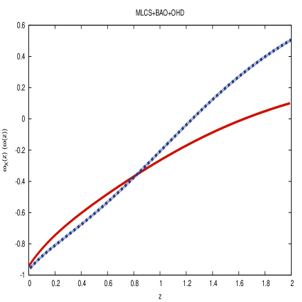
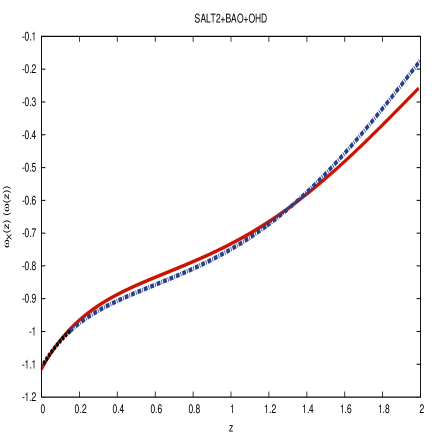
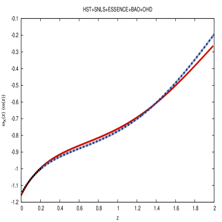
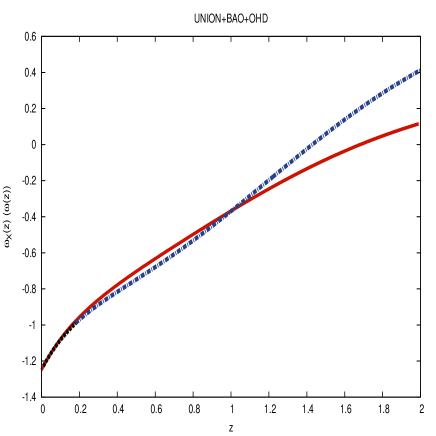
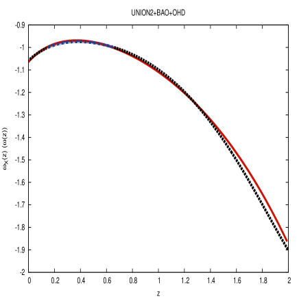
Figure 1: Comparison of $\omega(z)$ vs $z$ and $\omega_{X}(z)$ vs $z$ for the 5 data sets considered (see text). $\omega(z)$ ($\omega_{X}(z)$) are plotted along $y$ axis.

Using the formalism described in Sect. 4, the $\chi^{2}$ fit was performed [14] for each of the five sets of SNe Ia data alongwith BAO and OHD data and the best fit values of the parameters $a$, $b$ and $\Omega^{0}_{m}$ obtained for all the five sets [14]. The best fit parameters for each set (alongwith BAO and OHD) are given in Table 1. From the obtained best fit values of the parameters the equation of state $\omega_{X}(z)$ is computed using Eq. (6) and Eq. (31). Here we mention again, that no chosen form for $\omega_{X}(z)$ was adopted and $\omega_{X}(z)$ was obtained in a model independent way.

SNe Ia datasets		$a$		$b$		$\Omega_{m}^{0}$
(+BAO+OHD)
HST+SNLS+ESSENCE		1.437		0.550		0.268
(+BAO+OHD)
(Data Set I)
SALT2(+BAO+OHD)		1.401		0.542		0.272
(Data Set II)
MLCS(+BAO+OHD)		1.401		0.653		0.296
(Data Set III)
UNION(+BAO+OHD)		1.635		0.699		0.268
(Data Set IV)
UNION2(+BAO+OHD)		1.289		0.458		0.272
(Data Set V)

Table 1. Best fit values from analysis of different data sets

It is seen that except for Set I, for all other sets, $\omega_{X}(z)$ extends below the limit $\omega_{X}(z)=-1$ [14].

As discussed earlier, the dark energy equation of state ($\omega(z)$) is also formulated from a quintom scalar field model in this work. This model is based on the fact that when $\omega(z)>-1$ its nature can be described by assuming a potential $V(\phi)$ for a scalar field $\phi$ responsible for the dark energy. While in the scenario when $\omega(z)<-1$ the dark energy is described by a potential $V(\sigma)$ for a phantom field $\sigma$. This is described in Sections 3.3 and 4.1. Our purpose in this work is to compare dark energy equation of state ($\omega(z)$) from quintom scalar field model to that ($\omega_{X}(z)$) obtained from the data and check ow well the present formalism for dark energy can explain the variation of $\omega_{X}(z)$.

From the the best fit values of the parameters tabulated in Table 1, $d_{L}(z)$ and subsequently Hubble parameter $H(z)$ are computed. As discussed in Sect. 3.3, the fields $\phi(z)$ and $\sigma(z)$ can then be calculated using Eqs. (43,44). Consequently the chosen forms of $V(\phi)$ (= $\exp[\lambda_{1}(1+((\phi-\phi_{c})/M_{pl})^{2})]$) and $V(\sigma)$ (= $\exp[\lambda_{2}(1+((\sigma-\sigma_{0})/M_{pl})^{2})]$) are calculated for the particular case when $\lambda_{1}=\lambda_{2}=1$. The analyses of the five sets of data [14] indicate that for Set II $-$ Set V, we need to consider quintom scalar field (since $\omega_{X}(z)$ goes below $-1$) while from data set I only the quintessence field suffices.

It is argued earlier (Sect. 4.1) that $\phi(z)=\phi(z_{c})$, when $\omega_{X}(z)=-1$ and $\phi(z)=0$ at other values of $z<z_{c}$ for which $\omega_{X}(z)<-1$. Hence, $\phi(z_{c})$ is used instead of $\phi_{0}$ in the entire calculation for the case $z>z_{c}$. On the other hand, $\sigma_{0}$, the value of $\sigma(z)$ at $z=0$, remains undetermined and hence in our calculations, we rescale $\sigma(z)$ as ($\sigma(z)-\sigma_{0}$) and show our results.

We use the best fit values of the parameters given in Table 1 for all the five sets of data and compute $\omega(z)$ formulated from quintom model following Eqs. (11,18,30). These are done for different values of $z$ in the range $0<z<1.76$. For the present work, as stated earlier, $\lambda_{1}=1=\lambda_{2}$ is chosen in the expression of the potential $V(\phi)$. They are then compared with corresponding $\omega_{X}(z)$ for the five data sets, obtained from the $\chi^{2}$ fit and using Eqs (6, 40) [14]. The results are shown in Fig. 1.

In Fig. 1 the red coloured (solid line) plots represent the variation of $\omega_{X}(z)$ vs $z$ as obtained from the combined $\chi^{2}$ analyses of SNe Ia, BAO and OHD data [14]. The blue plots (dot-dashed line) in Fig. 1 are obtained from the calculation of $\omega(z)$ with the present formalism. As described earlier, for the first plot of Fig. 1 (corresponding to data set I), only quintessence scalar field describes the variation of $\omega(z)$ with the redshift $z$ since $\omega(z)>-1$, always, for this particular case. For the rest four plots the data analyses results show that $\omega_{X}(z)<-1$ for some redshift values. Hence for comparison with $\omega(z)$, the latter is calculated for quintom scalar field involving both $\phi(z)$ and $\sigma(z)$ for those four cases in Fig. 1 (corresponding to data Set II to Set V). In these four plots $\omega(z)$ from our calculations are given in bi-colour plots where the blue coloured dot-dashed line is obtained from the quintessence field $\phi(z)$ ($\omega(z)\geq-1$) and calculations with the phantom field ($\sigma(z)$) are represented by only black dashed line ($\omega(z)<-1$) of the plot.

From Fig. 1 one readily sees that the variations of the dark energy equation of states calculated using the adopted forms of $V(\phi)$ and $V(\sigma)$ in the present quintom scalar field formalism, are continuous. There are no discontinuities even when $\omega(z)$ varies from $\omega(z)>-1$ regime to the region where $\omega(z)<-1$. More importantly, it is also evident from Fig. 1 that the dark energy equation of states $\omega(z)$ calculated from the proposed quintom scalar field theory in the present work are in good agreements with $\omega_{X}(z)$ for at least three cases of data sets (namely Sets II, III and V) including the most recent UNION2 data set considered here. These results indicate that the proposed quintom scalar field formalism can be a viable model for explaining the varying dark energy.

References

- [1] A. G. Riess et al., Astron. J. 116, 1009 (1998), S. Perlmutter et al., Astrophys. J. 517, 565 (1999).
- [2] C. L. Bennett et al, Astrophys. J. Suppl. 148, 1 (2003), D. N. Spergel et al, Astrophys. J. Suppl. 148, 175 (2003).
- [3] M. Tegmark et al, Astrophys. J. 606, 702 (2004).
- [4] R. Jimenez and A. Loeb, Astrophys. J. 573 (2002) 37 [arXiv:astro-ph/0106145].
- [5] D. J. Eisenstein et al. [SDSS Collaboration], Astrophys. J. 633 (2005) 560 [arXiv:astro-ph/0501171].
- [6] A. G. Riess et al., Astrophys. J. 659, 98 (2007).
- [7] W. M. Wood-Vasey et al., Astrophys. J. 666, 694 (2007).
- [8] T. M. Davis et al., Astrophys. J. 666, 716 (2007).
- [9] M. Kowalski et al. Astrophys. J. 686, 749 (2008).
- [10] R. Kessler et al., Astrophys. J. Suppl. 185 , 32 (2009) [arXiv:0908.4274 [astro-ph.CO]].
- [11] R. Amanullah et al., Astrophys. J. 716, 712 (2010) [arXiv:1004.1711 [astro-ph.CO]].
- [12] Z. -K. Guo, Y. -S. Piao, X. -M. Zhang, Y. -Z. Zhang, Phys. Lett. B608 (2005) 177-182. [astro-ph/0410654].
- [13] T. Padmanabhan and T. R. Choudhury, Mon. Not. Roy. Astron. Soc. 344, 823 (2003).
- [14] D. Majumdar, A. Bandyopadhyay and D. Adak, J. Phys. Conf. Ser. 375, 032008 (2012).
- [15] L. Xu, Y. Wang, JCAP 1006 (2010) 002. [arXiv:1006.0296 [astro-ph.CO]].