Mean Interference in Hard-Core Wireless Networks

Abstract

Matérn hard core processes of types I and II are the point processes of choice to model concurrent transmitters in CSMA networks. We determine the mean interference observed at a node of the process and compare it with the mean interference in a Poisson point process of the same density. It turns out that despite the similarity of the two models, they behave rather differently. For type I, the excess interference (relative to the Poisson case) increases exponentially in the hard-core distance, while for type II, the gap never exceeds 1 dB.

I Introduction

I-A Motivation

Most analyses of performance of large ad hoc-type wireless networks is based on the stationary Poisson point process (PPP) [1]. However, the PPP is only an accurate model if the nodes are Poisson distributed and ALOHA is used as the MAC scheme. From a practical perspective, CSMA is much more important than ALOHA, but it is significantly more difficult to analyze since concurrent transmitters are spaced some minimum distance $\delta$ apart, which implies that the numbers of nodes in disjoint areas are no longer independent. The point processes used to model the transmitter set in CSMA are the Matérn hard-core processes of type I and type II. Both are based on a parent PPP of intensity $\lambda_{\rm p}$. In the type I process, all nodes with a neighbor within the hard-core distance $\delta$ are silenced, whereas in the type II process, each node has a random associated mark, and a node is silenced only if there is another node within distance $\delta$ with a smaller mark. Such hard-core processes are difficult to analyze, since their probability generating functionals do not exist (in contrast to clustered models, which are more tractable [2]). It has been argued in [3, 4] that the nodes further away than $\delta$ can still be modeled as a PPP, which would make the analysis of CSMA networks fairly tractable.

Our goal here is to verify the accuracy of the Poisson approximation by evaluating the mean interference measured at a typical node of the hard-core process. We shall see that only the type II process causes a level of interference comparable to the one in a PPP.

Other works on interference in CSMA networks include [5], where the mean interference is determined but at an arbitrary location on the plane rather than at a node of the point process, and [6], which uses simulations to find empirical distributions.

I-B Preliminaries

We first derive a general expression for the mean interference in networks whose nodes are distributed as a stationary point process $\Phi=\{x_{1},x_{2},\ldots\}\subset\mathbb{R}^{2}$ of intensity $\lambda$. For the path loss function $g(x)$, it is assumed that $\int_{\mathbb{R}^{2}}g(x)\mathrm{d}x<\infty$, Otherwise the interference is infinite a.s. for any stationary $\Phi$. The interference at the origin is defined as

$$I\triangleq\sum_{x\in\Phi}h_{x}g(x)\,,$$

where $h_{x}$ is the power fading coefficient associated with node $x$. It is assumed that $\mathbb{E}(h_{x})=1$ for all $x\in\Phi$. Rather than measuring interference at an arbitrary location in $\mathbb{R}^{2}$, we focus on the interference at the location of a node $x\in\Phi$, where it actually matters. Without loss of generality, due to the stationarity of the point process, we may take the node to be at the origin $o$. So the quantity of interest is $\mathbb{E}_{o}^{!}(I)$, which is the mean interference measured at $o$, given that $o\in\Phi$, but not counting this node’s signal power as interference. Using the reduced second moment measure $\mathcal{K}$ of the point process, we have [8]

$$\mathbb{E}_{o}^{!}(I)=\int_{\mathbb{R}^{2}}g(x)\mathcal{K}(\mathrm{d}x)\,.$$ (1)

For a radially symmetric path loss function, with a slight abuse of notation denoted as $g(\|x\|)\equiv g(x)$, and an isotropic point process, a polar representation is more convenient:

$$\mathbb{E}_{o}^{!}(I) =2\pi\int_{0}^{\infty}g(r)\mathcal{K}(r\mathrm{d}r)$$

$$=\lambda\int_{0}^{\infty}g(r)K^{\prime}(r)\mathrm{d}r\,.$$ (2)

The $K$-function is defined as $K(r)\triangleq\frac{1}{\lambda}\mathcal{K}(b_{o}(r))$, where $b_{o}(r)$ is the ball of radius $r$ centered at the origin $o$, so $K^{\prime}(r)\mathrm{d}r=\frac{2\pi}{\lambda}\mathcal{K}(r\mathrm{d}r)$. A central quantity in our study is the excess interference ratio (EIR), defined as follows:

Definition 1

The excess interference ratio (EIR) is the mean interference measured at the typical point of a stationary hard-core point process of intensity $\lambda$ with minimum distance $\delta$ relative to the mean interference in a Poisson process of intensity $\lambda(r)=\lambda\mathbf{1}_{[\delta,\infty)}(r)$.

$${\rm{EIR}}\triangleq\mathbb{E}_{o}^{!}(I)/\mathbb{E}_{o}^{!}(I_{\rm PPP})\,.$$ (3)

II Mean Interference in Hard-Core Processes

Hard-core processes have a guaranteed minimum distance $\delta$ between all pairs of points, which implies that $K(r)=0$ for $r<\delta$. In this section, we give tight bounds on the mean interference for Matérn processes of type I and II. We shall see that the Poisson approximation $K^{\prime}(r)=2\pi r\mathbf{1}_{[\delta,\infty)}(r)$ provides a rather tight lower bound for type II processes, while it gets increasingly loose as $\delta$ increases for type I processes.

II-A Matérn process of type I

Definition and $K$-function

In this point process, points from a stationary parent PPP of intensity $\lambda_{\rm p}$ are retained only if they are at distance at least $\delta$ from all other points [7]. The intensity of the resulting process is $\lambda=\lambda_{\rm p}\exp(-\lambda_{\rm p}\pi\delta^{2})$, and the $K$-function is

$$K(r)=2\pi\exp(2\lambda_{\rm p}\pi\delta^{2})\int_{0}^{r}uk(u)\mathrm{d}u\,,$$ (4)

where

$$k(u)=\begin{cases}0&u<\delta\\ \exp(-\lambda_{\rm p}V_{\delta}(u))&u\geq\delta\end{cases}$$ (5)

is the probability that two points at distance $u$ are both retained. It is easily verified that $K(r)\sim\pi r^{2}$ as $r\to\infty$, as is the case for all stationary point processes. $V_{\delta}(u)$ is the area of the union of two disks of radius $\delta$ whose centers are separated by $u$, given by

$$V_{\delta}(u)=2\pi\delta^{2}-2\delta^{2}\arccos\left(\frac{u}{2\delta}\right)+u\sqrt{\delta^{2}-\frac{u^{2}}{4}}\,,\;\;0\!\leq\!u\!\leq\!2\delta\,.$$

For $u>2\delta$, the union area is simply the area of the two disks, $2\pi\delta^{2}$. First we derive a lower bound on $K(2\delta)$, the mean number of nodes within distance $2\delta$ of the origin (not counting the node at the origin), normalized by the intensity. We have from (4)

$$K(2\delta)=8\pi\delta^{2}\int_{1/2}^{1}r\exp\Big{(}2\lambda\delta^{2}(\underbrace{\arccos r-r\sqrt{1-r^{2}}}_{f(r)})\Big{)}\mathrm{d}r\,.$$

Let $c=\pi/3+\sqrt{3}/4$. Since $f(r)\geq c-\sqrt{3}r$ for $1/2\leq r\leq 1$, replacing the upper integration bound by $c/\sqrt{3}<1$ (where the bound on $f(r)$ becomes zero), and replacing $r$ in the integrand by $1/2$ yields the lower bound

$$K(2\delta) >8\pi\delta^{2}\exp(2c\lambda_{\rm p}\delta^{2})\int_{1/2}^{c/\sqrt{3}}\frac{1}{2}\exp(-2\sqrt{3}\lambda_{\rm p}\delta^{2}r)\mathrm{d}r$$

$$=\frac{2\pi}{\sqrt{3}\lambda_{\rm p}}\left[\exp\bigg{(}\lambda_{\rm p}\delta^{2}\Big{(}\frac{2\pi}{3}-\frac{\sqrt{3}}{2}\Big{)}\bigg{)}-1\right]\,.$$ (6)

Hence the number of points within distance $2\delta$ of the typical point, normalized by the intensity, grows exponentially in $\delta^{2}$ and almost exponentially in $\lambda_{\rm p}$. For the PPP, $K(2\delta)\propto\delta^{2}$.

Similarly, for the derivative, we have from (4)

$$K^{\prime}(r)=2\pi\left(\frac{\lambda_{\rm p}}{\lambda}\right)^{2}rk(r)=2\pi\exp(2\lambda_{\rm p}\pi\delta^{2})rk(r)$$

with $k(r)$ defined as in (5). In particular,

$$K^{\prime}(\delta)=2\pi\delta\exp\bigg{(}\lambda\delta^{2}\Big{(}\frac{2\pi}{3}-\frac{\sqrt{3}}{2}\Big{)}\bigg{)}\,,$$

which shows that the node density in the annulus of inner radius $\delta$ and outer radius $\delta+\mathrm{d}r$ is higher than in the Poisson case by the factor $\exp(\lambda\delta^{2}(4\pi-3\sqrt{3})/6)\approx\exp(1.23\,\lambda\delta^{2})$. This suggests that the interference will be significantly larger also.

Interference bounds

Combining (2) and (4), the mean interference is

$$\mathbb{E}_{o}^{!}(I)=2\pi\lambda_{\rm p}\exp(\pi\lambda_{\rm p}\delta^{2})\int_{\delta}^{\infty}g(r)r\exp(-\lambda_{\rm p}V_{\delta}(r))\mathrm{d}r\,.$$

We split the interference into two terms, comprising the interference from the nodes closer than $2\delta$ and further than $2\delta$, respectively: $I=I_{<2\delta}+I_{>2\delta}$. We focus on $I_{<2\delta}$, i.e., the range $\delta\leq r\leq 2\delta$ first. In this range, $V_{\delta}(r)$ is increasing and concave, thus we obtain an upper bound from a first-order Taylor expansion at $r=3\delta/2$: Letting

$$\underline{a}\triangleq 2\arcsin\left(\frac{3}{4}\right)-\frac{3\sqrt{7}}{8}\,;\quad\underline{b}\triangleq\frac{\sqrt{7}}{2}$$

we have

$$V_{\delta}(r)<\left(\pi+\underline{a}\right)\delta^{2}+\underline{b}\delta r\,,\quad\delta<r<2\delta\,.$$ (7)

Since $\underline{a}<1/\sqrt{2}$ (but close), we could substitute $\underline{a}$ with $\underline{a}^{\prime}=1/\sqrt{2}$ to obtain a simpler yet almost equally tight bound. A lower bound on $V_{\delta}(r)$ is obtained by connecting the two points $V_{\delta}(\delta)=\delta^{2}(4\pi/3+\sqrt{3}/2)$ and $V_{\delta}(2\delta)=2\pi\delta^{2}$ by a straight line. This yields

$$V_{\delta}(r)>\left(\pi+\overline{a}\right)\delta^{2}+\overline{b}\delta r\,,\quad\delta<r<2\delta\,,$$ (8)

for

$$\overline{a}\triangleq\sqrt{3}-\frac{\pi}{3}\,;\quad\overline{b}\triangleq\frac{2\pi}{3}-\frac{\sqrt{3}}{2}\,.$$

To use these affine bounds on $V_{\delta}(r)$ to bound the mean interference, we define

$$h(a,b) \triangleq 2\pi\lambda_{\rm p}e^{-\lambda_{\rm p}a\delta^{2}}\int_{\delta}^{2\delta}g(r)re^{-\lambda_{\rm p}b\delta r}\mathrm{d}r$$

$$=2\pi\lambda_{\rm p}e^{-\lambda_{\rm p}a\delta^{2}}H(\lambda_{\rm p}b\delta,\delta)\,,$$ (9)

where $H(v,x)\triangleq\int_{x}^{2x}g(r)r\exp(-vr)\mathrm{d}r$. Upper and lower bounds on $\mathbb{E}_{o}^{!}(I_{<2\delta})$ can now be expressed as:

$$h(\underline{a},\underline{b})<\mathbb{E}_{o}^{!}(I_{<2\delta})<h(\overline{a},\overline{b})$$ (10)

Specializing to the class of power path loss laws $g(r)=(\max\{r_{0},r\})^{-\alpha}$, where $0\leq r_{0}\leq\delta$, there exists a concrete expression for $H$:

$$H(v,x)=v^{\alpha-2}\big{(}\Gamma(2-\alpha,vx)-\Gamma(2-\alpha,2vx)\big{)}\,.$$

Fig. 1 shows the bounds (10), normalized by the intensity $\lambda$, for $\alpha=3$ and $\lambda_{\rm p}=2$, as a function of $\delta$ (dashed curves).

The interference from nodes outside $r>2\delta$ is the same as in the (equi-dense) PPP:

$$\mathbb{E}_{o}^{!}(I_{>2\delta})=2\pi\lambda_{\rm p}\frac{\exp(-\lambda_{\rm p}\pi\delta^{2})}{(2\delta)^{\alpha-2}(\alpha-2)}$$

The total interference in the PPP is obtained by replacing the $2\delta$ in the denominator by $\delta$, hence $\mathbb{E}_{o}^{!}(I_{\rm PPP})=2^{\alpha-2}\mathbb{E}_{o}^{!}(I_{>2\delta})$. For the excess interference ratio, we find

$${\rm{EIR}}=\frac{1}{2^{\alpha-2}}\left(\frac{\mathbb{E}_{o}^{!}(I_{<2\delta})}{\mathbb{E}_{o}^{!}(I_{>2\delta})}+1\right)\,.$$ (11)

Theorem 1

For power path loss laws $g(r)$ with exponent $\alpha$, the excess interference in the Matérn process of type I grows exponentially, i.e.,

$${\rm{EIR}}=\Omega(e^{\lambda_{\rm p}\delta^{2}})\,,\quad\lambda_{\rm p}\delta\to\infty\,.$$ (12)

Proof:

Using the lower bound in (10),

$${\rm{EIR}}>e^{\lambda_{\rm p}\delta^{2}(\pi-\underline{a})}H(\lambda_{\rm p}\underline{b}\delta,\delta)(2\delta)^{\alpha-2}(\alpha-2)\,.$$

Since $H(v,x)\sim(vx^{\alpha-1}e^{vx})^{-1}$ as $\lambda_{\rm p}\delta\to\infty$,

$${\rm{EIR}}=\Omega\left(\frac{e^{\lambda_{\rm p}\delta^{2}(\pi-\underline{a}-\underline{b})}}{\lambda_{\rm p}\delta^{2}}\right)\,,\quad\lambda_{\rm p}\delta\to\infty\,.$$

The result follows from $\pi-\underline{a}-\underline{b}>1$. ∎

Keeping track of the pre-constants, we obtain an approximation, quite accurate for $\lambda_{\rm p}\delta^{2}>4$:

$${\rm{EIR}}\approx\frac{(\alpha-2)2^{\alpha-2}e^{\lambda_{\rm p}\delta^{2}(\pi-\underline{a}-\underline{b})}}{\lambda_{\rm p}\underline{b}\delta^{2}}$$ (13)

For the parameters in Fig. 1, at $\delta=2$, this yields 31.5dB.

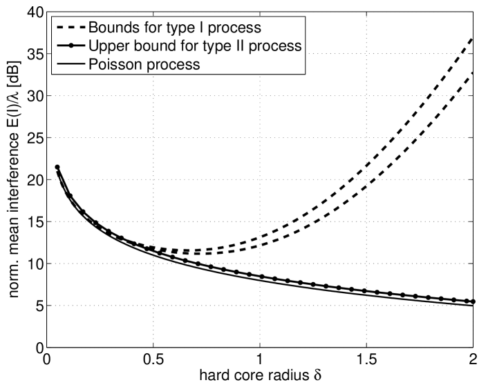
Figure 1: Normalized mean interference $\mathbb{E}_{o}^{!}(I)/\lambda$ for the Poisson point process (bottom solid curve), the upper bound from (15) for the Matérn process of type II (dotted solid curve), and upper and lower mean interference bound for the Matérn process of type I, for $\lambda_{\rm p}=2$ and $\alpha=3$. The EIR (gap) between the Poisson and type II curves is $0.5$ dB, while the gap between the Poisson and type I curves increases exponentially with $\lambda_{\rm p}$ and $\delta$. At $\delta=2$, the EIR is about 30dB.

II-B Matérn process of type II

Here, a random mark is associated with each point, and a point of the parent Poisson process is deleted if there exists another point within the hard-core distance $\delta$ with a smaller mark. The intensity of the resulting process is [7]

$$\lambda=\frac{1-\exp(-\lambda_{\rm p}\pi\delta^{2})}{\pi\delta^{2}}$$

and the probability that two points at distance $r$ are retained is, for $r\geq\delta$,

$$k(r)=\frac{2V_{\delta}(r)(1-e^{-\lambda_{\rm p}\pi\delta^{2}})-2\pi\delta^{2}(1-e^{-\lambda_{\rm p}V_{\delta}(r)})}{\lambda_{\rm p}^{2}\pi\delta^{2}V_{\delta}(r)(V_{\delta}(r)-\pi\delta^{2})}\,.$$

Theorem 2

Irrespective of the path loss function $g(r)$ and all other parameters, the excess interference ratio for Matérn processes of type II never exceeds

$$\nu\triangleq\frac{12\pi}{8\pi+3\sqrt{3}}<\frac{5}{4}<1{\rm dB}\,.$$ (14)

For power path loss laws with exponent $\alpha$, the bound can be sharpened to

$$\nu-\frac{\nu-1}{2^{\alpha-2}}\,.$$ (15)

Proof:

First we note that $(\frac{\lambda_{\rm p}}{\lambda})^{2}k(r)$ is monotonically increasing in $\lambda_{\rm p}$ and $\delta$ for all $\delta\leq r<2\delta$. For $r\geq 2\delta$, we have $(\frac{\lambda_{\rm p}}{\lambda})^{2}k(r)\equiv 1$, since outside distance $2\delta$ the hard-core process behaves like a PPP. This implies that the EIR can only increase with $\lambda_{\rm p}$ and $\delta$ (which is intuitive, since for $\lambda_{\rm p}\to 0$ or $\delta\to 0$, the process is Poisson). Hence letting $\lambda_{\rm p}\delta\to\infty$ yields an upper bound on the EIR. We have

$$k(\delta)\sim\frac{2}{\lambda_{\rm p}^{2}\pi\delta^{4}c}\,,\quad c\triangleq 4\pi/3+\sqrt{3}/2\,,$$

which upper bounds $k(r)$ for all $r\geq\delta$ and all finite $\lambda_{\rm p}$ and $\delta$. Consequently,

$$\frac{\mathbb{E}_{o}^{!}(I_{<2\delta})}{\lambda}<\int_{\delta}^{2\delta}2\pi g(r)\frac{\lambda_{\rm p}^{2}}{\lambda^{2}}\frac{2}{\lambda_{\rm p}^{2}\pi\delta^{4}c}r\mathrm{d}r=\int_{\delta}^{2\delta}g(r)\frac{4\pi^{2}}{c}r\mathrm{d}r\,,$$

where the RHS is $\nu=2\pi/c^{\prime}$ times the mean interference in the Poisson case. Inserting this bound into (11) yields the result for the power path loss law. ∎

For $\alpha=3$, this is quite exactly 0.5 dB, as reflected in Fig. 1.

III Conclusion

The behavior of two popular point process models for CSMA networks differs greatly. For the Matérn hard-core process of type I, the excess interference relative to the Poisson point process increases exponentially in the parent process density $\lambda_{\rm p}$ and the hard-core distance $\delta$ (for power path loss laws), while for Matérn processes of type II, the excess interference never exceeds 1dB, irrespective of the path loss law.

References

• [1] M.Β Haenggi, J.Β G. Andrews, F.Β Baccelli, O.Β Dousse, and M.Β Franceschetti, β€œStochastic Geometry and Random Graphs for the Analysis and Design of Wireless Networks,” IEEE Journal on Selected Areas in Communications, vol.Β 27, pp.Β 1029–1046, Sept. 2009.
• [2] R.Β K. Ganti and M.Β Haenggi, β€œInterference and Outage in Clustered Wireless Ad Hoc Networks,” IEEE Trans.Β on Information Theory, vol.Β 55, pp.Β 4067–4086, Sept. 2009.
• [3] A.Β Hasan and J.Β Andrews, β€œThe guard zone in wireless ad hoc networks,” IEEE Transactions on Wireless Communications, vol.Β 6, pp.Β 897–906, Mar 2007.
• [4] H.Β Q. Nguyen, F.Β Baccelli, and D.Β Kofman, β€œA Stochastic Geometry Analysis of Dense 802.11 Networks,” in IEEE INFOCOM, (Anchorage, AK), May 2007.
• [5] A.Β Busson, G.Β Chelius, and J.Β M. Gorce, β€œInterference Modeling in CSMA Multi-Hop Wireless Networks,” Tech. Rep. 6624, INRIA, Feb. 2009.
• [6] A.Β Busson and G.Β Chelius, β€œPoint Processes for Interference Modeling in CSMA/CA Ad Hoc Networks,” in Sixth ACM International Symposium on Performance Evaluation of Wireless Ad Hoc, Sensor, and Ubiquitous Networks (PE-WASUN’09), (Tenerife, Canary Islands, Spain), Oct. 2009.
• [7] B.Β MatΓ©rn, Spatial Variation. Springer Lecture Notes in Statistics, 2ndΒ ed., 1986.
• [8] M.Β Haenggi and R.Β K. Ganti, Interference in Large Wireless Networks. Foundations and Trends in Networking, NOW, 2008.