Possible Charge-Exchange X-Ray Emission in the Cygnus Loop Detected with Suzaku

Abstract

X-ray spectroscopic measurements of the Cygnus Loop supernova remnant indicate that metal abundances throughout most of the remnant’s rim are depleted to $\sim$0.2 times the solar value. However, recent X-ray studies have revealed in some narrow regions along the outermost rim anomalously “enhanced” abundances (up to $\sim$1 solar). The reason for these anomalous abundances is not understood. Here, we examine X-ray spectra in annular sectors covering nearly the entire rim of the Cygnus Loop using Suzaku (21 pointings) and XMM-Newton (1 pointing). We find that spectra in the “enhanced” abundance regions commonly show a strong emission feature at $\sim$0.7 keV. This feature is likely a complex of He-like O K($\gamma$ + $\delta$ + $\epsilon$), although other possibilities cannot be fully excluded. The intensity of this emission relative to He-like O K$\alpha$ appears to be too high to be explained as thermal emission. This fact, as well as the spatial concentration of the anomalous abundances in the outermost rim, leads us to propose an origin from charge-exchange processes between neutrals and H-like O. We show that the presence of charge-exchange emission could lead to the inference of apparently “enhanced” metal abundances using pure thermal emission models. Accounting for charge-exchange emission, the actual abundances could be uniformly low throughout the rim. The overall abundance depletion remains an open question.

1 Introduction

The importance of charge-exchange (CX) emission in X-ray astrophysics emerged with the discovery of bright X-ray emission from comet Hyakutake (Lisse et al. 1996) and the subsequent identification of its origin from CX processes between neutral atoms in the comet’s atmosphere and highly charged ions in the solar wind (Cravens et al. 1997). A number of comets are now known to have X-ray emission originating from CX processes (e.g., Cravens 2002). More recently, the diffuse soft X-ray background, which was previously thought to be dominated by thermal emission from the local hot bubble, turned out to be significantly contaminated by CX emission from interaction of heliospheric/geocoronal neutrals and solar wind ions (e.g., Cox 1998; Cravens 2000; Wargelin et al. 2004; Snowden et al. 2004; Lallement 2004a; Fujimoto et al. 2007; Smith et al. 2007; Koutroumpa et al. 2009; Ezoe et al. 2010).

In principle, CX-induced X-ray emission could be produced at any astrophysical site where hot plasma interacts with (partially) neutral gas. One very promising site is the thin post-shock layer in supernova remnants (SNRs), since SNR shocks are collisionless and both unshocked cold neutrals and shocked hot ions can be present just behind the shock front. In fact, observational evidence of CX emission has been obtained as the broad component of H$\alpha$ emission in many SNRs for more than 30 yrs (e.g., Chevalier et al. 1980; Ghavamian et al. 2001). On the other hand, CX-induced “X-ray” emission has not yet been detected firmly. It has been suggested only for the SMC SNR 1E0102.2–7219 (E0102) to explain anomalously high (in the context of thermal emission) intensity ratios of $\beta$/$\alpha$ and $\gamma$/$\beta$ in O VIII Ly series as observed by the XMM-Newton Reflection Grating Spectrometer (RGS) (Rasmussen et al. 2001). The authors suggested that CX processes at the reverse shock contribute significantly to the X-ray emission. However, Chandra High Energy Transmission Grating (HETG) observations (Flanagan et al. 2004) could not confirm the RGS result: the $\beta$/$\alpha$ ratio was found to be about two thirds of that measured by the RGS, consistent with that expected in thermal emission with an electron temperature of $\sim$0.5 keV. Although the detection of CX-induced X-ray emission from E0102 has been debated, other SNRs, especially nearby Galactic remnants, are more suitable for detecting it. Taking account of the CX emission could be extremely important for understanding the true properties of the shocked plasma, since the undetected presence of CX emission leads to incorrect plasma parameters (e.g., the metal abundance and the electron temperature) if we interpret the CX-contaminated X-ray spectra with pure thermal emission models. It should be also noted that CX reactions may be important for understanding magnetic-field amplification behind the shock front, a topic of continuing interest in SNR shock physics (Ohira et al. 2009; Ohira & Takahara 2010).

Unusual metal-abundance regions have been reported at the rim of the Cygnus Loop, which is a nearby (540 pc: Blair et al. 2005), extended (diameter of $\sim 2^{\circ}.8$: Levenson et al. 1998) SNR: the metal abundances in some of the outermost narrow (a few arcminutes, or $\lesssim$0.5 pc at a distance of 540 pc) rim regions are anomalously “enhanced” (up to about 1 solar, hereafter we define these abundances as “enhanced”, Katsuda et al. 2008ab; Tsunemi et al. 2009; Uchida et al. 2009; Kosugi et al. 2010), whereas the metal abundances are typically around 0.2 times the solar value for most of the rim (hereafter we define these abundances as “normal”, Miyata et al. 1999; Leahy 2004; Tsunemi et al. 2007; Miyata et al. 2007; Nemes et al. 2008; Zhou et al. 2010). Above and throughout this paper, we use the solar abundances of Anders & Grevesse (1989). The abundance ratios among metals in the “enhanced” abundance regions are consistent with solar values within a factor of $\sim$2. This fact, as well as the localization of the “enhancements” to a few regions along outermost rim, led the authors to suggest that the “enhancements” are not likely due to contamination by SN ejecta (Katsuda et al. 2008a). It is believed that the Cygnus Loop is a remnant from a core-collapse SN and that its forward shock is now hitting the wall of a wind-blown cavity over considerable fraction of the rim (e.g., McCray & Snow 1979; Hester et al. 1994; Levenson et al. 1997). Therefore, stellar winds might have altered abundances in part of the surroundings. However, stellar winds are expected to be rich in only lighter elements such as C, N, O, and Ne, as a result of CNO processing and/or He burning (e.g., Rauscher et al. 2002; Murashima et al. 2006), which is inconsistent with the overall abundance “enhancements”. It is also unlikely that the ISM abundances are inhomogeneous over such a small scale (a length scale of several pc), given that ISM abundances have been reported to be fairly constant in the local Galaxy. For example, Cartledge et al. (2004; 2006) revealed that the ISM abundances of a number of sight lines shorter than 800 pc are well within the measurement uncertainties, and concluded that the intrinsic rms scatter of the ISM abundances is $\sim$10%. A similar rms scatter of the ISM abundances was recently obtained from observations of nearby B stars (Przybilla et al. 2008). Since the Cygnus Loop, whose distance is 540${}^{+100}_{-80}$ pc (Blair et al. 2005), is within the region investigated, the abundance variation around the rim of the Cygnus Loop is difficult to understand. In addition to this problem, the “normal” abundances ($\sim$0.2 times the solar value) are also puzzling, given that the ISM metal abundances around the Cygnus Loop are about half the solar value (e.g., Cartledge et al. 2004).

Noting that the “enhanced” abundances are close to the ISM abundances, Katsuda et al. (2008b) and Tsunemi et al. (2009) suggested that the “normal” (i.e., depleted) abundances are only apparently low due to presence of a nonthermal component (power-law continuum), which can artificially raise the continuum level and thus decrease the equivalent widths of the lines. Indeed, introduction of a nonthermal component does increase the fitted abundances and yields slightly better overall spectral fits (the F-test probability of 99%). However, the radio flux inferred by the X-ray emission is unrealistic: it is required to be at least a few orders of magnitude higher than that observed. As a result, the authors speculated that there are indeed two kinds of material with different abundances: one is the ISM with “enhanced” abundances and the other, having the “normal” abundances, is the wall of the cavity surrounding the SN precursor. There is no good reason, however, why the ISM abundances should be elevated compared with those of the cavity wall, casting some doubt on this interpretation. Although some other possible explanations of the abundance enhancements and/or depletion, including dust depletion and resonance-line scattering, have been discussed in the literature (e.g., Katsuda et al. 2008b; Miyata et al. 2008; Uchida et al. 2009; Kosugi et al. 2010), none provides a satisfactory explanation.

In this paper, we suggest that the presence of CX emission is responsible for the abundance “enhancements” in the outermost rims of the Cygnus Loop. We present a new spatially-resolved X-ray spectral analysis of nearly the entire rim of the Cygnus Loop using Suzaku (21 pointings) and XMM-Newton (1 pointing). We argue that CX-induced X-ray emission is significant in the “enhanced” abundance regions and not in the “normal” abundance regions, and that it introduces apparent abundance enhancements when we apply pure thermal emission models to the CX-contaminated spectra.

2 Observations and Data Reduction

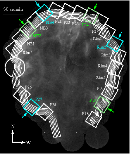
Figure 1: Logarithmically-scaled ROSAT HRI image of the entire Cygnus Loop. The image is binned by 5^′′ and has been smoothed by a Gaussian kernel of $\sigma=15^{\prime\prime}$. The FOV analyzed in this paper are shown as boxes for Suzaku and a circle for XMM-Newton. For convenience, we label Suzaku FOV according to the object name in the data file. Spectral extraction regions are indicated as narrow lines along the shock front. XIS spectra extracted from the outermost regions in the FOV in cyan (“enhanced” abundances) and green (“normal” abundances) are shown in Fig. 6.

We have observed nearly the entire rim region of the Cygnus Loop with Suzaku. In our analysis, we concentrate on the XIS data, since hard X-ray emission ($>$10 keV) from the Cygnus Loop is negligible. The fields of view (FOV) of the XIS pointings are shown as white boxes overlaid on the X-ray mosaic of the Cygnus Loop obtained by the ROSAT HRI (Fig. 1). We also analyze the XMM-Newton EPIC data. XMM-Newton’s FOV, which is indicated as a white circle in Fig. 1, partly covers the gap in the Suzaku observations along the eastern rim. Information about the observations is summarized in Table 1.

We reprocessed the XIS data using the 20090615 version of the CTI calibration file. We filtered the reprocessed data using the standard criteria recommended by the Suzaku/XIS calibration team. As for XMM-Newton, the raw data were processed using version 8.0.0 of the XMM Science Analysis Software (SAS). We selected X-ray events corresponding to patterns 0–12, and removed all the events in bad columns listed in Kirsch (2006). After the filtering, the data were vignetting-corrected using the SAS task evigweight. The effective exposure times for the various observations are listed in Table 1.

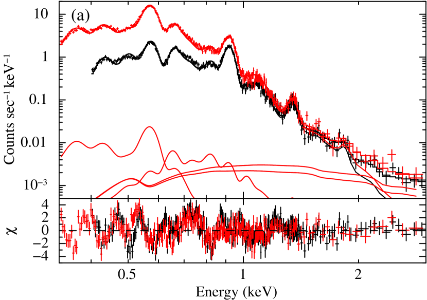
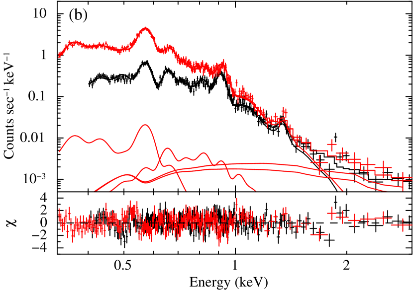
Figure 3: (a) XIS spectrum extracted from the NE4’s outermost rim along with the best-fit single temperature vpshock model. Black and red are the FI (XIS0+2+3) and BI (XIS1), respectively. Contributions of the X-ray backgrounds (see, text) are separately shown only for the BI data. The residuals are shown in the lower panel. (b): Same as left but for NE2.

Background in the XIS arises from two sources: non-X-ray background (NXB) caused by charged particles and $\gamma$-rays hitting the detectors, and diffuse X-ray background from the sky. We generate NXB spectra suitable for our observations using the xisnxbgen software (Tawa et al. 2008), and subtract them from the source spectra. The X-ray background was extensively studied by Yoshino et al. (2009) who modeled it as two thin thermal components plus one (or two) power-law component(s). They examined 15 blank-sky regions in various directions. Among these, the closest one to the Cygnus Loop located at ($\ell$, $b$)=(74^∘.0, -8^∘.5) is “Low Latitude 86–21” located at ($\ell$, $b$)=(86^∘.0, -20^∘.8). In our analysis, we model the X-ray background based on the spectral parameters for this blank-sky region. We note that the X-ray background is much weaker than the Loop emission (which will be shown in e.g., Fig. 3) and that the ROSAT all-sky survey shows generally similar backgrounds in these regions (Snowden, et al. 1997). Therefore, any differences in the background are negligibly small. The parameters of the background are taken from Table 4 in Yoshino et al. (2009) except for the total Galactic hydrogen column density which we modified to 1.7$\times$10²¹cm^-2 for the direction of the Cygnus Loop (Leiden/Argentine/Bonn Survey of Galactic HI, Kalberla et al. 2005). For the EPIC background, we use the data set accumulated from blank sky observations prepared by Read & Ponman (2003). We subtract the blank-sky data from the source after matching the detector coordinates.

3 Comparison of “Enhanced” and “Normal” Abundance Regions

As described in the introduction, there are apparent abundance inhomogeneities along the rim of the Cygnus Loop: overall, the abundance is typically 0.2 times the solar value, while parts of the outermost rim show “enhanced” abundances of up to $\sim$1 solar. Our investigation of the nature of the enhancement starts by summarizing observational properties of the rim regions.

3.1 Spectral Properties

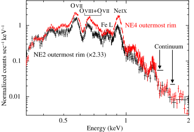
Figure 2: Two FI (XIS0+2+3) spectra extracted from the outermost rim regions in the NE2 (black) and the NE4 (red). The NE2 spectrum is multiplied by 2.33 so that the count rate in the continuum band (1.4–1.5 keV and 1.65–1.75 keV) is equalized to that in the NE4 spectrum. The O and Ne enhancement in the NE4 spectrum is readily seen.

First, we compare a typical “enhanced” abundance spectrum with a “normal” one. To this end, we focus on the XIS data for the NE rim, because these were obtained in the early phase of the Suzaku mission, and have the best photon statistics as well as the best spectral resolution among all the data listed in Table 1. These data were previously analyzed by Katsuda et al. (2008a), who divided each FOV into small box regions, and found “enhanced” abundances in the outermost regions in NE3 and NE4. They also found that the parameters are generally constant with azimuth (along the shock front). Therefore, to make the comparison with better statistics, we here extract azimuthally-integrated spectra from narrow regions (thickness of 2^′) along the shock front in each FOV as shown in Fig. 1. Figure 2 shows spectra extracted from the outermost regions in NE4 (for the “enhanced” abundance region) and NE2 (for the “normal” abundance region). These spectra are normalized to each other in the energy bands of 1.4–1.5 keV and 1.65–1.75 keV where line features are not evident. The differences between the two are readily seen: K-shell lines from O and Ne are significantly enhanced in NE4 relative to those in NE2, whereas the complex of Fe L-shell lines at $\sim$0.82 keV is comparable in the two spectra.

To confirm previous fitting results, we fit the two spectra with an absorbed, single component, plane-parallel shock model [a combination of the Tbabs (Wilms et al. 2000) and the vpshock model (NEI version 2.0) (e.g., Borkowski et al.  2001) in XSPEC v 12.5.1]. This thermal emission model is the same as that employed in Katsuda et al. (2008b). We assume the hydrogen column density of the intervening material to be 3$\times 10^{20}$ cm^-2 (e.g., Kosugi et al. 2010). Note that this value is much smaller than the total Galactic column density of 1.7$\times$10²¹cm^-2 for the direction of the Cygnus Loop (see, Section 2) because of the proximity of the Loop. We freely vary the electron temperature, $kT_{\mathrm{e}}$, the ionization timescale, $n_{\rm e}t$, and the volume emission measure (VEM $=\int n_{\mathrm{e}}n_{\mathrm{H}}dV$, where $n_{\mathrm{e}}$ and $n_{\mathrm{H}}$ are number densities of electrons and protons, respectively, and $V$ is the X-ray–emitting volume). Above, $n_{\rm e}t$ is the electron density times the elapsed time after shock heating, and the model uses a range from 0 up to a fitted maximum value. The abundances of several elements, whose line emission is prominent in the spectrum, are treated as free parameters: C, N, O, Ne, Mg, Si (=S), Fe (=Ni). We manually adjust the energy scale within the systematic uncertainties to obtain better fits, by allowing energy-scale offsets to vary freely for the front illuminated (FI) and the back illuminated (BI) detectors, respectively. In this way, we fit the spectra in energy ranges of 0.4–3.0 keV for FI and 0.33–3.0 keV for BI. Figure 3 shows the best-fit model along with the data points. The best-fit parameters are summarized in Table 2. We confirm that the absolute (relative to H) abundances are enhanced in NE4 compared with those in NE2, and that the abundance ratios of C/Fe, N/Fe, O/Fe, and Ne/Fe are $\sim$2–4 times higher in NE4 than those in NE2. We also confirm that the plasma is in the non-equilibrium ionization (NEI) condition ($n_{\mathrm{e}}t<10^{12}$ cm^-3 sec^-1). Dividing the ionization timescale by the time elapsed after shock heating, which is roughly inferred from the distance of $\sim 1\times 10^{18}$ cm (i.e., 2^′ at a distance of 540 pc) divided by the fluid velocity of $\sim$200 km sec^-1 (e.g., Salvesen et al. 2009), we estimate the post-shock electron densities in NE4 and NE2 to be $\sim$1 cm^-3 and $\sim$6 cm^-3, respectively. Assuming strong shocks, we can estimate the pre-shock ambient densities in NE4 and NE2 to be $\sim$0.25 cm^-3 and $\sim$1.5 cm^-3, respectively. These values generally agree with previous estimates (e.g., Raymond et al. 2003 for NE4; Hester et al. 1994 for NE2), showing the robustness of the ionization timescales derived in these outermost rim regions from the very shock fronts to 2^′ inside the shocks.

We notice that the fit quality for the NE4 spectrum is far from formally acceptable (reduced $\chi^{2}$ of $\sim$2.2), while the fit quality for the NE2 spectrum is much better. The NE4 spectrum in Fig. 3 (a) shows apparent excess emission at $\sim$0.7 keV relative to the best-fit model. This discrepancy was already noticed in the Chandra analysis of the NE rim (Katsuda et al. 2008b), although it was not so evident due to poorer statistics. We therefore re-fit the NE4 spectrum using the same model, but ignoring the energy band 0.68–0.76 keV. Table 2 (the 3rd column) summarizes the best-fit parameters. The fit quality is significantly improved over the original one (the reduced-$\chi^{2}$ is reduced from 2.2 to 1.6). Both the electron temperature and the abundances significantly decrease from the original best-fit values to values more consistent with those in NE2 (the 2nd column in Table 2). These changes are interpreted as follows. In the original (entire energy band) fitting, the He-like O K-shell lines ($n\geq 4\to n=1$) which dominate around 0.7 keV are forced to be as strong as possible to match excess emission in the 0.68–0.76 keV band. The way these lines are made stronger is by an increase in the electron temperature as well as the O abundance. When this energy band is disregarded in the fit, the electron temperature decreases from $\sim$0.3 keV to $\sim$0.2 keV. The reduced temperature in turn allows a reduced O abundance, since the emissivities of O K-shell lines peak at $kT_{\mathrm{e}}\sim$0.2 keV. Other metal abundances are also reduced, with the net result that the relative abundances among metals are maintained. Therefore, we conclude that the 0.68–0.76 keV band plays an important role in determining absolute abundances in the “enhanced” abundance spectrum when using the Suzaku XIS or any other CCD spectrometers. For the “normal” abundance spectrum (e.g., the NE2 spectrum in Fig. 3 (b)), ignoring the 0.68–0.76 keV band does not change the fit quality or the best-fit parameters.

In order to compare the two spectra in more detail, we next fit them with a phenomenological model consisting of an absorbed, bremsstrahlung continuum plus a number of Gaussians for line emission from C, N, O, Ne, Mg, Si, and Fe. Again, we assume the hydrogen column density to be 3$\times 10^{20}$ cm^-2. We include eight Gaussians for the prominent line features at $\sim$0.35 keV (C Ly$\alpha$), $\sim$0.45 keV (C Ly$\beta$ $+$ N He$\alpha$), $\sim$0.5 keV (N He$\beta$ $+$ N Ly$\alpha$), $\sim$0.57 keV (O He$\alpha$), $\sim$0.91 keV (Ne He$\alpha$), 1.35 keV (Mg He$\alpha$), $\sim$1.6 keV (Mg He$\beta$), and $\sim$1.85 keV (Si He$\alpha$). The center energies of these lines are allowed to vary freely. In addition to these, we introduce nine Gaussians to represent lines that could contribute in the crowded 0.7–1.2 keV band. These are O Ly$\alpha$ at 0.654 keV, O He$\beta$ at 0.666 keV, an Fe XVII L-shell complex from the 3s$\to$2p transitions at 0.726 keV, O Ly$\beta$ at 0.775 keV, an Fe XVII L-shell complex from the 3d$\to$2p transitions at 0.822 keV, Ne Ly$\alpha$ at 1.022 keV, Ne He$\beta$ at 1.074 keV, Ne He$\gamma$ at 1.127 keV, and Ne Ly$\beta$ at 1.210 keV. The line center energies of these nine Gaussians are fixed at their theoretically expected values (APED: Smith et al. 2001). Based on the most recent NEI plasma code (Borkowski et al. 2001; the augmented NEI version 2.0 that includes inner-shell processes), the intensity ratio between overall Fe L-shell 3s$\to$2p and 3d$\to$2p lines is fairly constant at unity. Therefore, we assume the normalization of the Gaussian for the 3s$\to$2p transition lines to be the same as that for the 3d$\to$2p transition lines. We manually adjust the energy scale within the systematic uncertainty. In this way, we fit the two spectra shown in Fig. 2. As expected from the spectral fitting in the previous paragraphs, we find excess emission from the best-fit model at $\sim$0.7 keV for the “enhanced” abundance spectrum. Addition of a Gaussian at $\sim$0.7 keV gives a satisfactory fit; the statistical significance of introducing the line is greater than 99.9% for both spectra (reduced-$\chi^{2}$ values are reduced from 1297 to 601 for NE4 and from 440 to 404 for NE2).

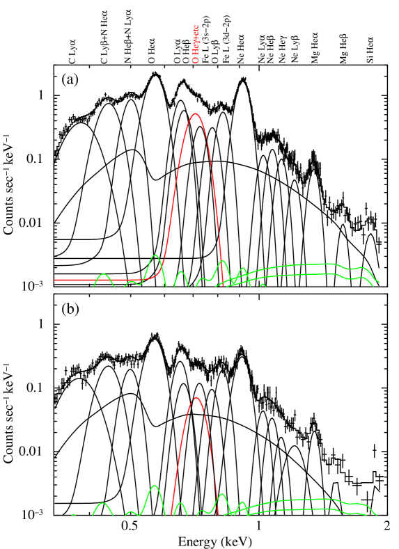
Figure 4: (a) NXB-subtracted FI (XIS0+2+3) spectrum from the NE4’s outermost rim (FI only) along with the best-fit model consisting of a bremsstrahlung plus 18 Gaussians. Line identifications are shown on top of the panel. Green curves show individual contributions of the X-ray background. (b) Same as above but for the NE2’s outermost rim.

The electron temperatures of the bremsstrahlung components are 0.16$\pm$0.01 keV and 0.26$\pm$0.01 keV for NE2 and NE4, respectively. Although we do not consider radiative recombination continuum emission or two-photon decay continuum emission, the electron temperatures derived are reasonable for the rim of the Cygnus Loop. Table 3 summarizes details of this model. The line center energies listed in the table include the effects of energy-scale shifts determined by the fittings. Figure 4 presents the best-fit models. We find that the line intensities in NE4 are generally $\sim$3 times higher than those in NE2, whereas the line at $\sim$0.7 keV indicated as a red line in Fig. 4 is $\sim$7 times stronger in NE4 than in NE2. Its nonzero width suggests that it is a complex of lines, although we cannot fully eliminate the possibility that the broadening might be due to calibration effects.

3.2 Spatial Properties

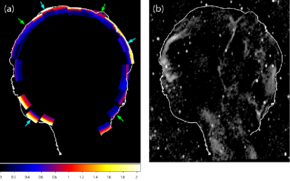
Figure 5: (a) Line-ratio map of the $\sim$0.7 keV emission to the Fe L-shell complex at $\sim$0.82 keV. The X-ray boundary of the Cygnus Loop is shown as a white line. Arrows indicate the regions where we show the XIS spectra in Fig. 6. (b) Logarithmically-scaled radio (325 MHz) surface brightness map obtained by the WENSS team (Rengelink et al. 1997), with the X-ray boundary of the Cygnus Loop as in Fig. 5 (a).

Before proceeding to an investigation of the origin of the $\sim$0.7 keV feature, we briefly summarize the spatial properties of the $\sim$0.7 keV emission. To reveal the distribution of the $\sim$0.7 keV feature, we fit all the spectra for all the regions in Fig. 1 using the same phenomenological model as we employed in Section 3, a bremsstrahlung plus 18 Gaussians. We show example best-fit values for the outermost rim regions in P27, P19, Rim2, and P24 in Table 3. After deriving individual line intensities in each region, we calculate the line ratio between the $\sim$0.7 keV emission and the Fe L-shell complex at $\sim$0.82 keV. This ratio should be a good tracer of the relative strength of the $\sim$0.7 keV emission, given that the abundance (and intensity) of Fe (L-shell complex) is relatively constant in the rim regions (see, e.g., Fig. 2). Figure 5 (a) shows this line-ratio map, with the X-ray boundary of the Cygnus Loop in white. The map clearly shows that the $\sim$0.7 keV emission is enhanced exclusively within a narrow ($\lesssim 4^{\prime}$) layer behind the shock.

Also notable from Fig. 5 (a) is the azimuthal variation. The $\sim$0.7 keV emission is evident only at position angles of 0^∘–40^∘ (N–NE), 110^∘–160^∘ (SE), and 270^∘–330^∘ (northwest: NW) measured from north over east. These are the same locations as where the “enhanced” abundances have been reported so far (N–NE by Katsuda et al. 2008ab and Uchida et al. 2009; SE by Tsunemi et al. 2009 and Kosugi et al. 2010). In addition, preliminary spectral analysis of the NW region shows “enhanced” abundances at the outermost regions compared with those in the inner regions (Takakura et al. in preparation). Therefore, it appears that the “enhanced” abundance regions commonly show the strong $\sim$0.7 keV emission. We further note that a map of the intensity ratio of Ne He$\alpha$ to the Fe L-shell complex at $\sim$0.82 keV is quite similar to Fig. 5 (a), and that the intensity-ratio enhancements seen in part of the region (which corresponds to the “enhanced” abundance regions) are statistically significant.

Figure 5 (b) shows a 325 MHz radio image of the Cygnus Loop from the The Westerbork Northern Sky Survey (WENSS) (Rengelink et al. 1997) covering the same sky region of Fig. 5 (a). Looking at Fig. 5 (a) and (b), we notice that the regions of strong $\sim$0.7 keV emission are generally anti-correlated with radio-bright regions.

4 Discussion

4.1 Identification of Excess 0.7 keV Emission in the “Enhanced” Abundance Regions

In this section, we discuss the origin of the $\sim$0.7 keV emission feature. The center energy of the $\sim$0.7 keV feature suggests that it is most likely either O K-shell emission or Fe XVII/XVI L-shell emission. We first consider Fe XVII. In the X-ray band, there are two well-known strong Fe L-shell complexes at $\sim$0.73 keV and $\sim$0.82 keV, which mostly arise from the 3s$\to$2p and the 3d$\to$2p transitions in Fe XVII ions, respectively. While these two complexes are included in the phenomenological model above, the intensities of the two were set equal, based on the most up-to-date plasma code (Borkowski et al. 2001). This assumption leaves room for the 3s$\to$2p complex to contribute to the $\sim$0.7 keV complex, given the moderate spectral resolution of the XIS (FWHM$\sim$60 eV at 1 keV). However, the energy of the 3s$\to$2p complex is $\sim$0.73 keV, making it unlikely to be the dominant source of the $\sim$0.7 keV emission, the center energy of which is 0.705$\pm 0.002_{\mathrm{stat}}\pm 0.005_{\mathrm{sys}}$ keV (the systematic uncertainty is from Koyama et al. 2007). In addition, if we attribute the entire intensity of the $\sim$0.7 keV emission to the 3s$\to$2p complex, the intensity ratio of 3s$\to$2p/3d$\to$2p would be $\sim$3.5. Such a high ratio has never been observed in an astrophysical object. Although astrophysical sources including stellar coronae, SNRs, and elliptical galaxies do tend to show higher 3s$\to$2p/3d$\to$2p ratios than the predicted value (Doron & Behar 2002 and references therein), the observed ratio ranges from 1 to 2. Our own analyses at XMM-Newton RGS observation of the LMC SNRs DEM L71, N103B, N132D, N49, and N63A reveal that the 3s$\to$2p/3d$\to$2p intensity ratio in each is near or less than unity. Therefore, we rule out 3s$\to$2p emission from Fe XVII as the origin of the $\sim$0.7 keV feature.

Turning to Fe XVI L-shell lines, Graf et al. (2009) recently reported relative intensities, using University of California / Lawrence Livermore National Laboratory’s EBIT-I. In the energy range of 0.69–0.86 keV, the authors measured ten Fe XVI lines originating from innershell ionization processes. Among them, the strongest one is located at $\sim$0.82 keV, whereas four relatively weak lines are clustered around 0.7 keV. The total intensity of the lines around 0.7 keV is weaker than that around 0.82 keV. This measurement is inconsistent with our measured line ratio: the $\sim$0.7 keV emission is $\sim$2.5 times stronger than the $\sim$0.82 keV emission (which should include both the Fe XVI L-shell lines and the Fe XVII 3d$\to$2p complex). It is therefore unlikely that the Fe XVI L-shell lines dominate the $\sim$0.7 keV emission, although we cannot fully exclude this possibility given that these lines will incidentally be stronger in an NEI plasma than in a collisional ionization equilibrium plasma.

Finally, we consider the possibility that O VII K-shell lines ($n\geq 4\to n=1$) produce the $\sim$0.7 keV emission. In this case, we again run into a line ratio problem for a thermal spectrum: the intensity ratio of the $\sim$0.7 keV emission to O He$\alpha$ is measured to be $\sim$0.06 (see, the parameters in Table 3), whereas the O He($\gamma+\delta$) to O He$\alpha$ ratio is expected to be $\sim$0.02 at $kT_{\mathrm{e}}=0.2$ keV based on the NEI code (Borkowski et al. 2001). Therefore, it is also unlikely that thermally-emitted O VII K-shell lines are responsible for the $\sim$0.7 keV emission.

4.2 Charge-Exchange Emission

We suggest here that a pure NEI plasma model is not appropriate for reproducing the $\sim$0.7 keV emission in the “enhanced” abundance region, and that an additional emission mechanism is required. One possible emission mechanism, suggested from the interpretation of the XMM-Newton RGS spectrum of the SMC remnant E0102 (Rasmussen et al. 2001), is CX-induced emission between neutrals and ions at the forward shock of the Cygnus Loop.

CX emission would play an important role only in a thin region immediately behind the forward shock in a SNR, because cold neutrals cannot survive far behind the shock. Taking account of line-of-sight effects, CX emission if present could only be detected at the periphery of a SNR. This is exactly what the line ratio map in Fig. 5 (a) shows.

In general, the presence of neutral hydrogen is essential for CX emission to be significant. The presence of neutral hydrogen in the post-shock region can be tested by the presence/absence of non-radiative H$\alpha$ filaments. Such filaments are found around nearly the entire perimeter of the Cygnus Loop (Levenson et al. 1998), clearly indicating the presence of neutral hydrogen in the post-shock regions. One H$\alpha$ filament along the NE rim was extensively studied by Ghavamian et al. (2001), who modeled the broad and narrow components of the H$\alpha$ and H$\beta$ emission with their shock model to measure the degree of electron-ion temperature equilibration. In their model, the neutral fraction in the ambient medium is also a measurable parameter, although not a sensitive one. They examined three cases of neutral fractions, i.e., 0.1, 0.5, and 0.9, to model the broad-to-narrow line ratios, and found that the first case is slightly outside the range of the observational uncertainties whereas the latter two are consistent with the observation. Thus, the preferred range for the neutral fraction is larger than 0.1 in this region.

With non-radiative H$\alpha$ filaments around nearly the entire periphery, and a non-zero neutral fraction, it might be expected that the CX emission should be closely correlated with the non-radiative filaments. However, it does not seem to be the case. One possible explanation for distribution of CX emission is suggested by the radio map (Fig. 5). The regions of the rim from which the hypothetical CX emission is not detected generally correspond to those that are radio bright. The radio emission is likely produced by accelerated cosmic-rays (electrons), since the spectral shape of the radio emission is well described by a power-law continuum (e.g., Uyaniker et al. 2004). Therefore, the anti-correlation can be qualitatively understood in a view that the cosmic-ray shock precursor more effectively pre-ionizes the medium, and thus reduces the CX emission below a detectable level. It is also interesting to note that the radio-bright (or CX-absent) regions correspond to radiative filaments (Levenson et al. 1998). This correspondence suggests that the ambient densities there are higher and the shock velocities are lower than elsewhere along the rim. According to Lallement (2004b), slower shocks produce less CX emission, providing another possible explanation for the observed azimuthal variation of the CX emission. It may be also possible that thermal emission overwhelms CX emission in these radio/optical-bright regions.

All of these observations support the possibility of CX emission in the “enhanced” abundance regions. Furthermore, a major benefit of this scenario is that the introduction of CX emission resolves the mysterious abundance “enhancements” in the outermost rim regions, by reducing the “enhanced” abundances to consistency with the “normal” abundances found everywhere else around the rim. We therefore suggest that CX emission is contributing significantly to the X-ray spectrum in the “enhanced” abundance regions.

We note that if this suggestion is to hold, CX emission other than the $\sim$0.7 keV complex is expected to be present. As pointed out in Section 3.2, the similarity of a map of the intensity ratio of Ne He$\alpha$ to the Fe L-shell complex to Fig. 5 suggests that Ne He$\alpha$ is also contaminated by CX-induced lines. In addition, under the condition of the electron temperature of $\sim$0.2 keV, C is likely fully ionized and thus H-like C emission due to CX processes would be also significant. CX strongly enhances high principal number Ly emission such as C Ly$\gamma$ at $\sim$0.46 keV (Wargelin et al. 2008). This emission can contaminate the C Ly$\beta+$N He$\alpha$ blend around 440 eV (see, Table 3). Therefore, the line intensity ratio of this blend to C Ly$\alpha$ may be enhanced where we find indications of CX. However, such a trend can not be detected as shown in Table 3. A definitive identification of the possible CX lines would require higher spectral resolution observations which will be soon available by the Soft X-ray Spectrometer (SXS) with the energy resolution of 4–7 eV and the energy calibration of 1–2 eV (Mitsuda et al. 2010) onboard the Astro-H satellite (Takahashi et al. 2010).

4.3 Supporting Evidence for CX Emission

4.3.1 Spectral Modeling of CX Emission

In order to further study the properties of the proposed CX emission, we model CX-contaminated spectra by a combination of a number of Gaussians for the CX emission and a plane parallel shock model (the vpshock model; Borkowski et al. 2001) for the thermal emission. We examine three spectra extracted from the outermost rim regions in NE4, P27, and Rim2 where the possible CX emission is fairly strong (see, Fig. 5). The challenge is the difficulty in separating CX emission from thermal emission in CCD spectra. Detailed modeling considering the effects of CX on the ionization balance or evolution of the electron temperature is far beyond the scope of this paper. We here crudely assume that the shape of the thermal emission in this region is similar to that in its surroundings, so that we can estimate the thermal emission in the CX-contaminated spectra. Since the thermal spectra are expected to be more constant with azimuth than with the distance from the shock front, we use the thermal spectrum extracted from the outermost rim in observation fields where we do not find indications of CX emission. As a template of thermal emission, we take the NE2 spectrum shown in Figs. 2 and 3. The best-fit spectral parameters are listed in Table 2. It should be noted that recombination rates of ions increase due to CX processes and thus plasmas showing CX emission may be in lower ionization states than those showing pure thermal emission. However, it is quite difficult to estimate this effect quantitatively. We thus evaluate systematic uncertainties by examining two ionization timescales: one is the value derived in the NE2 spectrum and the other is half the value.

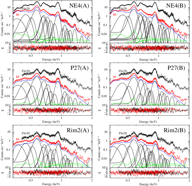
Figure 6: Top panels: NE4’s outermost rim spectra (black and red for the FI and BI data, respectively) along with the best-fit model consisting of an assumed vpshock component (blue), 22 Gaussians (black), and the X-ray background (green). Contributions of these components are separately shown only for the BI data. The vpshock component in the left panel has the same spectral parameters derived in the NE2’s outermost rim (see, Table 2), whereas that in the right panel has half the value for the ionization timescale. Middle and bottom panels: Same as top panels but for P27 (middle) and Rim2 (bottom).

In the fitting, we fix all the thermal parameters except for the emission measures (EM $=\int n_{\mathrm{e}}n_{\mathrm{H}}d\ell$, where $\ell$ is the plasma depth). We introduce 22 Gaussians to represent possible CX line emission. These are K-shell lines from C, N, O, Ne, Mg, and Si. For simplicity of the model, we ignore Fe L-shell lines that might be significant in the X-ray band. For example, Fe L-shell lines may affect intensities of the O Ly($\beta+\gamma+\delta+\epsilon$) around 0.8 keV, given that the heliospheric/geocoronal solar-wind charge-exchange (SWCX) emission shows a hint of an Fe L-shell complex around $\sim$0.8 keV (Snowden et al. 2004; Fujimoto et al. 2007; Smith et al. 2007). Therefore, the inferred intensities of O Ly($\beta+\gamma+\delta+\epsilon$) should be considered to be upper limits. This model gives us statistically acceptable fits for all the cases examined. Figure 6 shows the best-fit model and the residuals. In the figure, left (labeled A) and right (labeled B) columns present results for the vpshock model with the $n_{\mathrm{e}}t$-value of 2.8$\times 10^{11}$ cm^-3 sec^-1 (see, Table 2) and that with half the value, respectively. The best-fit EMs (not shown in Table 4) are obtained to be $\sim$3$\times 10^{19}$ cm^-5 for NE4, $\sim$2.3$\times 10^{19}$ cm^-5 for P27, $\sim$1.4$\times 10^{19}$ cm^-5 for Rim2, respectively.

In order to clarify improvements from the initial fit with the pure thermal emission model (Fig. 3 (a)), we show the NE4 spectrum with the initial (pure thermal) model in Fig. 7 (a) and the new (thermal plus possible CX lines) model in Fig. 7 (b), focusing on a small spectral region around the possible CX lines of interest (i.e., 0.68–0.76 keV). It is clear from this figure that the new model fits the data much better than the initial one. For quantitative evaluation of the goodness-of-fits, we perform Kolmogorov-Smirnov (K-S) test for the two fit results shown in Fig. 7 (a) and (b). We find that the probabilities that the data are drawn from the initial and new best-fit models are $\sim$15% and $\sim$80%, respectively. Therefore, the new model is much better than the initial one, although both models cannot be fully ruled out according to this K-S test. We also re-fit the data in a wide energy band using a maximum likelihood method, and compute the Bayesian Information Criterion (BIC) defined as $\chi^{2}+k$ln($n$), where $k$ is the number of free parameters and $n$ is the number of spectral bins. The BIC-value is lower for the new model than the initial one, which also shows the validity for introducing possible CX lines.

Table 4 summarizes the best-fit Gaussian parameters, from which the intensity ratios of O He($\gamma+\delta+\epsilon$) / O He$\alpha$ are calculated to be $\sim$0.097–0.110 in NE4, $\sim$0.057–0.061 in P27, and $\sim$0.066–0.090 in Rim2. These are much higher than that expected for the thermal emission from the Cygnus Loop ($\sim$0.02 is expected at $kT_{\mathrm{e}}\sim 0.2$ keV), but are also larger than those expected in CX emission (the ratio is likely to be $\sim$0.04; Beiersdorfer et al. 2003; Wargelin et al. 2005). These inconsistencies imply that our modeling is not perfect and requires further sophistication which is beyond the scope of this paper. Here, it may be worth noting that the ratios derived in our primitive modeling are closer to CX emission than to thermal emission, lending support to the idea that CX emission is present.

Using the line intensities listed in Table 4, we next estimate ion number ratios in the plasma, as performed for SWCX emission (e.g., Kharchenko et al. 2003; Krasnopolsky 2004; Snowden et al. 2004). We limit our estimation to only O VIII, O IX, and Ne X, whose line intensities (K-shell lines from O VII, O VIII, and Ne IX after CX reactions) are relatively well constrained. From Table 4, the intensity ratios of O VIII lines / O VII lines and Ne IX lines / O VII lines are calculated to be $\sim$0.095–0.184 and $\sim$0.079–0.086 in NE4, $\sim$0.006–0.026 and $\sim$0.059–0.069 in P27, and $\sim$0.052–0.156 and $\sim$0.040–0.053 in Rim2, respectively. Above, we summed K-shell fluxes from all transitions in the same species, since the total number of K-shell photons reflects the number of CX reactions. To convert the flux ratios to ion number ratios, we use SWCX cross sections for hydrogen listed in Wargelin et al. (2004). The cross section ratios of O IX / O VIII and Ne X / O VIII are computed to be 1.66 and 1.53, respectively. Dividing the flux ratios by the cross section ratios, the ion number ratios for O IX / O VIII and Ne X / O VIII are derived to be $\sim$0.057–0.111 and $\sim$0.052–0.056 in NE4, $\sim$0.004–0.016 and $\sim$0.039–0.045 in P27, and $\sim$0.031–0.094 and $\sim$0.026–0.035 in Rim2, respectively.

We compare these ion number ratios with those expected in the thermal plasma of the Cygnus Loop’s rim, i.e., $kT_{\mathrm{e}}$=0.2 keV. We investigate three ionization timescales: $n_{\mathrm{e}}t$ = (0.5, 1, 2)$\times$10¹¹ cm^-3 sec. As described in the appendix, the ion number ratios for O IX / O VIII and Ne X / O VIII are derived to be $<$0.33 and 0.01–0.02, respectively (here, we adopt the Ne/O abundance ratio of 2 times the solar value which is typically reported in the Cygnus Loop, e.g., Tsunemi et al. 2007). Although the error range is large for the former ratio, it is consistent with our estimates ranging from $\sim$0.004 to $\sim$0.111 using SWCX cross sections. On the other hand, the latter ratio is significantly lower than our measurement by a factor of $\sim$1.3–5.6. This discrepancy suggests either overestimates of CX lines from He-like Ne, underestimates of CX lines from H-like O, or both. The overall intensity of O VIII lines is also somewhat uncertain because of the difficulty in separating O Ly$\alpha$ at 0.654 keV and O He$\beta$ at 0.666 keV as well as the possible contribution of Fe L-shell lines around 0.8 keV. Based on the best-fit parameters in Tables 3 (total emission) and 4 (CX emission), the fractions of CX emission in total emission are calculated to be $\sim$40% for O He$\alpha$ and $\sim$50% for Ne He$\alpha$. A higher fraction of CX emission in Ne He$\alpha$ than in O He$\alpha$ is difficult to understand, since the fraction of H-like ions (which yield He$\alpha$ CX emission) is higher for O than for Ne; at the electron temperature of $\sim$0.2 keV in thermal equilibrium, a little less than half of O is He-like, while less than 10% of Ne is H-like and the rest is He-like. Taking account of NEI effects would make things worse. Therefore, Ne He$\alpha$ CX lines are likely to be overestimated by our primitive CX modeling. This problem could be caused by inaccurate modeling of the thermal emission, because the line ratios strongly depend on the plasma condition which is difficult to infer in the CX-contaminated spectra. In addition to the uncertainty in the spectral modeling, the CX cross sections might be different from those we employed. Given these complexities, the derivation of accurate ion number ratios from CX emission is left for future work. At the very least, we can argue here that the ion fractions inferred from both CX emission and the thermal emission model are consistent within an order of magnitude.

4.3.2 CX Emission from SNRs

Although it is challenging to distinguish between CX emission and thermal emission in our data, we have constructed a spectral model for the CX emission, assuming that spectral shape of the thermal emission is similar with azimuthal angle. We here discuss the inferred CX-to-thermal flux ratios (e.g., O He$\alpha\sim$40%) in terms of theoretical expectations.

Wise & Sarazin (1989) were the first to perform detailed calculations of CX-induced X-ray emission in a SNR. They found that CX emission generally contributes only 10^-3 to 10^-5 of the collisionally excited lines in the entire SNR, even when the ambient gas is completely neutral. For comparison, we estimate the total CX-to-thermal flux ratio in the Cygnus Loop. We assume that the total CX flux is 10 times larger than that in Table 4 for NE4, since the number of FOV where we see CX emission is about ten (see, Fig. 5 (a)). The total thermal flux from the remnant is likewise inferred from the integrated thermal flux in all the spectral extraction regions in Fig. 1. The CX-to-thermal ratio in the entire SNR is then inferred to be on the order of 10^-2, which is significantly higher than that in the model of Wise & Sarazin (1989). This discrepancy requires either a reduction of the CX contribution in our spectral modeling in Section 4.3.1, improvements of the theoretical calculation, or perhaps both. In fact, physical parameters such as the shock velocity used in the calculation by Wise & Sarazin (1989) are different from those in the Cygnus Loop.

More recently, Lallement (2004b) investigated spatial variations of CX emission in a SNR. According to Fig. 3 in Lallement (2004b), CX emission can comprise a few 10% of the total X-ray (0.1–0.5 keV) emission within the radius of $0.98R_{\mathrm{shock}}<R<R_{\mathrm{shock}}$, which corresponds to the outermost rim region in our analysis. This theoretical prediction agrees reasonably well with our measurement of O He$\alpha\sim$40%. Although Lallement’s calculation is specifically intended for the LMC SNR DEM L71, we believe that it is appropriate for a qualitative comparison with the Cygnus Loop, since the basic parameters for both the DEM L71 SNR and the Cygnus Loop are similar.

Lallement (2004b) also presented the expected EM of thermal emission at the equivalent radius, i.e., the radius where the flux of CX emission becomes equal to that of the thermal emission. The expected EM is expressed as 2$\times 10^{17}$ $\epsilon$ cos${}^{-1}\theta$ $\alpha$ $\chi$(T,a)^-1 $n_{\mathrm{c}}$ V₁₀₀ cm^-5, where $\epsilon$ is the ratio between the CX probability and the collisional ionization probability, $\theta$ is an incidence angle (see, Fig. 2 in Lallement 2004b), $\alpha$ accounts for the hot ion content, i.e., the temperature and metallicity, $\chi$(T,a) is the thermal emissivity ratio for a given temperature T and the metal abundance a relative to a temperature 1$\times$10⁶ K and the solar abundance, $n_{\mathrm{c}}$ is the ambient density, and V₁₀₀ is the relative velocity between neutrals and the hot gas in units of 100 km sec^-1. Following the discussion in Lallement (2004b), we employ $\epsilon=1$, $\alpha=1$, and $\chi$(T,a)$=1$. The equivalent radius of $\sim 0.98R_{\rm shock}$, which is the inner edge of the outermost region in Fig. 1 gives us cos${}^{-1}\theta$ of $\sim$5. The ambient density is taken to be unity from measured values ranging from 0.3 to 4 cm^-3 near NE4 (Raymond et al. 2003; Leahy 2003). The relative velocity can be considered as the shock velocity of $\sim$300 km sec^-1 (Ghavamian et al. 2001; Salvesen et al.  2009). Substituting these quantities in the equation above, we derive the expected EM of $\sim 5\times 10^{18}$ cm^-5. Since the EM observed in the outermost rim in NE4 is estimated to be $\sim$1.4–3 $\times$10¹⁹ cm^-5 (see, Section 4.2.1), the expected and observed EMs are consistent within a factor of $\sim$2–6. Given the considerable uncertainties in the spectral modeling as well as the ambient density, we believe that the EMs are in reasonable agreement.

We have found general agreements between our observational results and the theoretical predictions by Lallement (2004b). Nonetheless, further detailed calculation of the CX emission in a SNR is encouraged, since Lallement’s calculation is somewhat simplified in that it does not consider the ionization structure of the post-shock region, and thus would lead to an overestimate of the CX contribution. Likewise, more sophisticated spectral modeling of CX emission is also desirable for future work.

4.4 Need for High-Resolution Spectra with the Astro-H SXS

While we have proposed CX emission for the origin of the “enhanced” abundance in the rim regions of the Cygnus Loop and have presented supporting observational evidence, solid evidence for the presence of CX emission is still missing. Therefore, at this point, we cannot fully exclude alternative explanations. For example, there could really be a bimodal distribution of abundances in the rim of the Cygnus Loop, in spite of the difficulties described in Section 1.

The Astro-H SXS will hopefully provide definitive evidence for CX emission by resolving the O He$\alpha$ triplets, i.e., resonance, intercombination, and forbidden lines. In thermal emission, the ratio of forbidden to resonance line strengths is less than unity. In contrast, for CX emission the ratio is expected to be about 10 (Kharchenko et al. 2003). Laboratory measurements of CX reactions do show stronger forbidden lines than resonance lines (Beiersdorfer et al. 2003), although the forbidden-to-resonance ratio is not as large as 10 (which might be related to the fact that the authors used CO₂ rather than H as electron-donor species). Thus, we expect that forbidden lines will be enhanced in the CX-contaminated outermost rim regions compared with those in the rest of the rim. So far, the northern bright portion of the Cygnus Loop is the only location where the triplets have been resolved, by high spectral resolution Einstein Focal Plane Crystal Spectrometer (FPCS) observations (Vedder et al. 1986). The resonance line there is much stronger than the forbidden line, suggesting that CX emission is not significant. Since the FPCS FOV (3${}^{\prime}\times$30^′) is located well outside (or inside with respect to the center of the Loop) our Suzaku FOV shown in Fig 1, it is reasonable to consider that signatures of CX emission if present would be washed out by thermal emission. Spatial variations of the line ratio, which provide the key information about the presence of CX emission, will be measured with the Astro-H SXS.

With the current CCD data, it might be possible to find a forbidden/resonance line-ratio variation by measuring the energy separation between O He$\alpha$ and O Ly$\alpha$ (e.g., Lallement 2009). However, such energy separations are expected to be less than a few eV, and thus are too small to detect with nondispersive CCD spectra. As we show in Tables 3 and 4, the fit line center energies in the Suzaku spectra are randomly scattered within the energy-scale calibration uncertainties ($\pm$5 eV: Koyama et al. 2007). Moreover, O Ly$\alpha$ is significantly contaminated by O He$\beta$ in part of the Cygnus Loop, and its contribution is highly variable from location to location. This makes even more difficult any firm measurement of the separation between O He$\alpha$ and O Ly$\alpha$. Also, dispersed spectra from slitless X-ray grating spectrometers are almost useless for the Cygnus Loop because of its large extent, although the XMM-Newton RGS might provide better spectra for some bright knotty features. Since the Astro-H SXS is a nondispersive microcalorimeter, it will be the first instrument to provide us with high-resolution spectra of sufficient quality to resolve individual lines of the triplets. The high-resolution spectra will also make possible identification of the individual lines around 0.7 keV. Therefore, the Astro-H SXS is being eagerly awaited for further studies of the Cygnus Loop.

In addition, the Astro-H SXS will help us derive much more accurate absolute metal abundances than those from nondispersive CCD spectra. This is because we can directly measure equivalent widths of lines below 1 keV with SXS spectra, which is not possible with CCD spectra.

While measuring the absolute abundance with CCD spectra is quite difficult, it should be noted that relative metal abundances are already well constrained unless the spectra are heavily contaminated by CX emission. Our analysis suggests that CX emission is not significant in the “normal” abundance regions. The relative abundances obtained there are close to the solar ratio except for O: the abundance of O is depleted by an additional factor of 2 relative to other elements (e.g., Miyata et al. 1994). As Miyata et al. (2008) pointed out, the depletion of the O abundance might be due to resonance-line scattering which is especially important for O K-shell lines. Therefore, in order to obtain accurate absolute and relative abundances in the rim of the Cygnus Loop, we will need to carefully consider effects of both CX emission and resonance-line scattering.

5 Conclusion

Using Suzaku and XMM-Newton data covering nearly the entire rim of the Cygnus Loop, we found that outermost rims in N–NE, SE, and NW regions show a strong line feature at $\sim$0.7 keV. Its anomalously strong intensity and spatial localization in the outermost rim lead us to propose that it originates from CX processes, most likely between neutrals and H-like O ions. If so, this is the first detection of CX-induced X-ray emission associated with the forward shock of a SNR. The regions showing the $\sim$0.7 keV emission correspond to the “enhanced” abundance regions, and we suggest that the $\sim$0.7 keV emission and possibly other CX lines could enhance the apparent metal abundances there when we fit the CX-contaminated spectra with pure thermal emission models. The introduction of the CX emission potentially resolves the mysterious abundance “enhancements” in the outermost rim regions of the Cygnus Loop. On the other hand, the abundance depletion in overall rim regions still remains an open question.

6 Appendix

To estimate the ion fractions, we first calculate ion fractions at collisional ionization equilibrium using sherpa. Second, we calculate $n_{z}$/$n_{\mathrm{Z}}$$\epsilon_{i}(T)$ (i.e., a product of ion fraction and emissivity) of some selected lines as a function of $n_{\mathrm{e}}t$, using the NEIline software provided by R. Smith (applications of this software can be found in literature, e.g., Sasaki et al. 2004; Katsuda & Tsunemi 2006). Above, $n_{z}(n_{\mathrm{e}}t)$/$n_{\mathrm{Z}}$ is the ionization fraction of the ionization species responsible for the line, and $\epsilon_{i}(T)$, a function of temperature, is the intrinsic emissivity of the line. Then, assuming that the $\epsilon_{i}(T)$ is constant with $n_{\mathrm{e}}t$, we roughly estimate ion fractions at various $n_{\mathrm{e}}t$-values. To evaluate systematic uncertainties associated with this method, we use not only K$\alpha$ lines but also K$\beta$ lines. This method does not directly give ion fractions for fully ionized ions, since they do not radiate line emission by collisional excitation. We thus assume that fully ionized ions take up the balance, which is a good approximation in the plasma condition of interest.

Table 1: Summary of observations.

Obs. ID	Obs. Date	R.A., Decl. (J2000)	Position Angle	Effective Exposure
500020010 (NE1)	2005-11-23	20h56m45s.24, 31∘44′16′′.8	223∘.0	20.4 ksec
500021010 (NE2)	2005-11-24	20h55m52s.34, 31∘57′15′′.1	223∘.0	21.4 ksec
500022010 (NE3)	2005-11-29	20h55m01s.99, 32∘10′57′′.4	222∘.9	21.7 ksec
500023010 (NE4)	2005-11-30	20h54m00s.12, 32∘22′08′′.4	221∘.2	25.3 ksec
501020010 (P10)	2007-11-26	20h46m17s.86, 30∘23′57′′.1	240∘.0	16.8 ksec
501035010 (P18)	2006-12-18	20h48m13s.13, 29∘42′40′′.0	237∘.5	12.0 ksec
501036010 (P19)	2006-12-18	20h47m14s.26, 30∘04′54′′.5	237∘.5	18.6 ksec
503057010 (P21)	2008-06-02	20h52m47s.04, 32∘25′10′′.9	61∘.9	16.2 ksec
503058010 (P22)	2008-06-03	20h51m20s.47, 32∘24′16′′.9	61∘.4	19.3 ksec
503059010 (P23)	2008-06-03	20h49m54s.53, 32∘21′31′′.3	61∘.9	19.5 ksec
503060010 (P24)	2008-06-04	20h48m32s.16, 32∘17′25′′.8	61∘.4	18,5 ksec
503061010 (P25)	2008-06-04	20h47m26s.59, 32∘10′04′′.1	60∘.9	26.0 ksec
503062010 (P26)	2008-05-13	20h56m30s.05, 30∘18′48′′.6	49∘.8	16.9 ksec
503063010 (P27)	2008-05-13	20h55m19s.87, 30∘00′37′′.4	49∘.6	22.8 ksec
503064010 (P28)	2008-05-14	20h53m55s.13, 29∘53′36′′.2	49∘.1	18.2 ksec
504005010 (Rim1)	2009-11-17	20h46m34s.10, 31∘52′58′′.8	60∘.0	40.7 ksec
504006010 (Rim2)	2009-11-18	20h45m42s.24, 31∘35′40′′.6	60∘.0	26.3 ksec
504007010 (Rim3)	2009-11-19	20h45m17s.57, 31∘17′57′′.5	246∘.4	21.6 ksec
504008010 (Rim4)	2009-11-20	20h45m52s.27, 31∘00′47′′.2	246∘.0	12.1 ksec
504009010 (Rim5)	2009-11-20	20h46m06s.86, 30∘40′52′′.7	216∘.0	15.9 ksec
504010010 (Rim6)	2009-11-20	20h57m30s.50, 31∘27′01′′.1	220∘.0	14.3 ksec
0018141301 (XMM-Newton)	2002-04-30	20h57m21s.02, 31∘00′13′′.3	262∘.4	11.2 ksec

Table 2: Spectral-fit parameters in the outermost regions of NE4 and NE2, using the absorbed vpshock model.

Parameter	NE4	NE4 (ignoring 0.68–0.76 keV)	NE2
$N_{\mathrm{H}}$[$\times 10^{22}$cm-2]	0.03 (fixed)	0.03 (fixed)	0.03 (fixed)
$kT_{\mathrm{e}}$[keV]	0.34${}^{+0.01}_{-0.03}$	0.22$\pm$0.01	0.21$\pm$0.01
log$(n_{\mathrm{e}}t_{\mathrm{upper}}/\mathrm{cm}^{-3}\,\mathrm{sec})$	10.77${}^{+0.11}_{-0.03}$	11.41${}^{+0.06}_{-0.03}$	11.44${}^{+0.10}_{-0.08}$
C	0.85${}^{+0.11}_{-0.22}$	0.20${}^{+0.02}_{-0.04}$	0.17${}^{+0.04}_{-0.03}$
N	0.88${}^{+0.11}_{-0.25}$	0.15${}^{+0.02}_{-0.03}$	0.07$\pm$0.02
O	0.43${}^{+0.05}_{-0.11}$	0.12${}^{+0.01}_{-0.02}$	0.08$\pm$0.01
Ne	0.75${}^{+0.09}_{-0.16}$	0.29${}^{+0.02}_{-0.03}$	0.15$\pm$0.02
Mg	0.29${}^{+0.04}_{-0.05}$	0.12$\pm$0.02	0.10${}^{+0.03}_{-0.04}$
Si(=S)	0.22${}^{+0.11}_{-0.12}$	$<$0.11	$<$0.10
Fe(=Ni)	0.38${}^{+0.05}_{-0.09}$	0.11$\pm$0.01	0.14$\pm$0.02
EMa[$\times 10^{19}$ cm-5]	0.36${}^{+0.20}_{-0.04}$	2.9${}^{+0.5}_{-0.2}$	1.5$\pm$0.3
Energy shifts[eV]	$+$0.4 (FI), $-$1.7 (BI)	$+$0.4 (FI), $-$1.7 (BI)	$-$2.9 (FI), $+$0.2 (BI)
$\chi^{2}$/d.o.f.	1219/551	802/505	466/410

Note. — ^aEM denotes the emission measure ($=\int n_{\mathrm{e}}n_{\mathrm{H}}d\ell$). The values of abundances are multiples of the solar values (Anders & Grevesse 1989). The errors represent 90% confidence ranges.

Table 3: Gaussian parameters in the NE4, NE2, P27, P19, Rim2, and P24’s outermost rims, using an absorbed phenomenological model consisting of an underlying bremsstrahlung plus 18 Gaussians.

Line	NE4a	NE2	P27a	P19	Rim2a	P24
C Ly$\alpha$
Center (eV)	357(357)${}^{+2}_{-3}$	351(354)$\pm 5$	349(351)$\pm 8$	349(345)$\pm 6$	349(356)$\pm 3$	347(348)$\pm 6$
Width (eV)	28$\pm$2	30$\pm$3	32${}^{+3}_{-5}$	32${}^{+2}_{-4}$	30$\pm$2	29${}^{+3}_{-4}$
Normalizationb	7606${}^{+568}_{-405}$	3215${}^{+309}_{-324}$	7998${}^{+500}_{-1363}$	9550${}^{+482}_{-1289}$	7074${}^{+396}_{-504}$	5421${}^{+456}_{-778}$
C Ly$\beta$ + N He$\alpha$
Center (eV)	438(438)$\pm$1	437(441)$\pm$2	435(438)${}^{+2}_{-4}$	432(429)$\pm$2	435(442)$\pm$3	433(434)${}^{+3}_{-5}$
Width (eV)	14${}^{+1}_{-2}$	14$\pm$3	14${}^{+4}_{-2}$	14${}^{+2}_{-3}$	11${}^{+3}_{-7}$	9${}^{+6}_{-10}$
Normalizationb	2023${}^{+51}_{-63}$	591${}^{+32}_{-18}$	1779${}^{+128}_{-116}$	2239${}^{+126}_{-127}$	958${}^{+83}_{-90}$	822${}^{+95}_{-75}$
N Ly$\alpha$ + N He$\beta$
Center (eV)	499(499)${}^{+1}_{-2}$	497(501)${}^{+0}_{-4}$	499(501)${}^{+2}_{-4}$	499(496)${}^{+1}_{-2}$	499(506)${}^{+2}_{-3}$	495(496)${}^{+3}_{-2}$
Width (eV)	0c	0c	0c	0c	0c	0c
Normalizationb	730$\pm$20	177$\pm$12	481$\pm$38	686$\pm$39	281$\pm$23	257$\pm$25
O He$\alpha$
Center (eV)	565(565)$\pm$0	564(567)$\pm$1	564(567)$\pm$1	565(561)$\pm$1	564(571)$\pm$1	563(564)$\pm$1
Width (eV)	12$\pm$0	12$\pm$1	13$\pm$1	11${}^{+1}_{-2}$	12$\pm$1	12${}^{+1}_{-2}$
Normalizationb	5547${}^{+53}_{-55}$	1659$\pm$34	4763${}^{+98}_{-106}$	4559${}^{+97}_{-105}$	2804${}^{+62}_{-59}$	2243${}^{+69}_{-70}$
O Ly$\alpha$
Center (eV)	654(653)c	651(655)c	653(655)c	653(649)c	653(660)c	651(652)c
Width (eV)	0c	0c	0c	0c	0c	0c
Normalizationb	602$\pm$17	208$\pm$10	258$\pm$28	607$\pm$32	259$\pm$16	178$\pm$18
O He$\beta$
Center (eV)	666(665)c	663(667)c	665(667)c	665(661)c	665(672)c	663(664)c
Width (eV)	0c	0c	0c	0c	0c	0c
Normalizationb	367$\pm$16	82$\pm$9	444$\pm$26	437$\pm$29	130$\pm$14	194$\pm$16
O He$\gamma+$etc.
Center (eV)	704(704)$\pm$2	708(711)${}^{+7}_{-8}$	703(706)$\pm$5	711(708)$\pm$6	705(712)${}^{+4}_{-5}$	718(719)${}^{+8}_{-9}$
Width (eV)	22$\pm$2	20${}^{+11}_{-10}$	24${}^{+5}_{-6}$	23$\pm$7	23${}^{+5}_{-6}$	0${}^{+24}_{-0}$
Normalizationa	341${}^{+17}_{-16}$	48${}^{+10}_{-9}$	239${}^{+28}_{-27}$	206${}^{+31}_{-29}$	145${}^{+16}_{-15}$	47${}^{+14}_{-9}$
Fe L (3d$\to$2p)
Center (eV)	726(725)c	723(727)c	725(727)c	725(721)c	725(732)c	723(724)c
Width (eV)	0c	0c	0c	0c	0c	0c
Normalizationb	Linked to Fe L (3d$\to$2p)
O Ly$\beta$
Center (eV)	775(774)c	772(776)c	774(776)c	774(770)c	774(781)c	772(773)c
Width (eV)	0c	0c	0c	0c	0c	0c
Normalizationb	99$\pm$6	35$\pm$4	54$\pm$8	134$\pm$12	38$\pm$5	42$\pm$6
Fe L (3s$\to$2p)
Center (eV)	822(822)$\pm$1	819(823)${}^{+1}_{-2}$	819(821)${}^{+2}_{-3}$	822(818)${}^{+2}_{-3}$	822(829)${}^{+3}_{-2}$	819(820)$\pm$2
Width (eV)	0c	0c	0c	0c	0c	0c
Normalizationb	138$\pm$4	57$\pm$3	93$\pm$6	247$\pm$9	67$\pm$4	64$\pm$4
Ne He$\alpha$
Center (eV)	912(912)$\pm$1	909(912)${}^{+1}_{-2}$	913(915)$\pm$1	912(908)$\pm$1	915(921)$\pm$1	912(913)$\pm$2
Width (eV)	15$\pm$1	19$\pm$2	13$\pm$2	15$\pm$2	14$\pm$2	13${}^{+3}_{-4}$
Normalizationb	364${}^{+5}_{-6}$	89${}^{+4}_{-3}$	282$\pm$8	337$\pm$10	140$\pm$4	111$\pm$5
Ne Ly$\alpha$
Center (eV)	1022(1021)c	1019(1023)c	1021(1023)c	1021(1017)c	1021(1028)c	1019(1020)c
Width (eV)	0c	0c	0c	0c	0c	0c
Normalizationb	16$\pm$2	7$\pm$1	12$\pm$2	26$\pm$3	7$\pm$1	10$\pm$2
Ne He$\beta$
Center (eV)	1074(1073)c	1071(1075)c	1073(1075)c	1073(1069)c	1073(1080)c	1071(1072)c
Width (eV)	0c	0c	0c	0c	0c	0c
Normalizationb	19$\pm$1	5$\pm$1	15$\pm$2	16$\pm$3	7$\pm$1	6$\pm$1
Ne He$\gamma$
Center (eV)	1127(1126)c	1124(1128)c	1126(1128)c	1126(1122)c	1126(1133)c	1124(1125)c
Width (eV)	0c	0c	0c	0c	0c	0c
Normalizationb	12$\pm$1	2$\pm$1	8$\pm$2	17$\pm$3	5${}^{+1}_{-2}$	5$\pm$1
Ne Ly$\beta$
Center (eV)	1210(1209)c	1207(1211)c	1209(1211)c	1209(1205)c	1209(1216)c	1207(1208)c
Width (eV)	0c	0c	0c	0c	0c	0c
Normalizationb	5$\pm$1	3$\pm$1	7$\pm$2	5${}^{+3}_{-2}$	4$\pm$1	4$\pm$1
Mg He$\alpha$
Center (eV)	1341(1341)$\pm 4$	1346(1350)$\pm 5$	1354(1356)$\pm 11$	1343(1339)$\pm 5$	1350(1357)$\pm 7$	1346(1347)$\pm 8$
Width (eV)	12 ($<$19)	0 ($<$31)	36${}^{+35}_{-22}$	6 ($<$22)	27${}^{+10}_{-13}$	39${}^{+39}_{-13}$
Normalizationb	8.2$\pm$1.1	2.9$\pm$1.0	6.2${}^{+1.4}_{-1.5}$	9.9$\pm$1.8	4.8${}^{+1.0}_{-1.1}$	6.6$\pm$1.3
Mg He$\beta$
Center (eV)	1571(1571)$\pm 17$	1511(1514)$\pm 38$	1522(1525)$\pm 381$	1578(1574)$\pm 395$	1574(1581)$\pm 394$	1576(1577)$\pm 394$
Width (eV)	0c	0c	0c	0c	0c	0c
Normalizationb	1.2$\pm$0.8	0.5 ($<$1.2)	1.52${}^{+1.0}_{-1.2}$	1.2 ($<$2.4)	0.8 ($<$1.6)	0.9 ($<$1.8)
Si He$\alpha$
Center (eV)	1833(1833)${}^{+25}_{-26}$	1886(1889)$\pm 22$	1839(1841)$\pm 57$	1865(1861)$\pm 18$	1872(1879)$\pm 37$	1806(1808)$\pm 43$
Width (eV)	0c	0c	0c	0c	0c	0c
Normalizationb	1.3$\pm$0.9	0.8 ($<$1.7)	1.4 ($<$2.4)	2.8${}^{+2.5}_{-1.3}$	1.5${}^{+1.0}_{-1.1}$	1.1$\pm$0.9

Note. — ^a”Enhanced”-abundance regions. ^bIn units of photons cm^-2 s^-1 sr^-1. ^bFixed values. Line center energies include effects of energy shifts determined by the fittings. Values in parentheses are derived from the BI CCD. The errors (90% confidence level) are estimated with the other Gaussian parameters and the bremsstrahlung parameters fixed at the best-fit values. These errors do not include systematic uncertainties, such as $\pm$5 eV for the line center energies (Koyama et al. 2007).

Table 4: Gaussian parameters for the possible CX emission in the NE4, P27, and Rim2’s outermost rims, using an absorbed combination model consisting of the vpshock plus 22 Gaussians.

Line	NE4		P27		Rim2
	A	B	A	B	A	B
C Ly$\alpha$
Center (eV)	343(343)$\pm 13$	—	345(347)$\pm 17$	—	330(337)${}^{+11}_{-6}$	313(320)${}^{+17}_{-9}$
Width (eV)	30${}^{+29}_{-10}$	—	30${}^{+29}_{-11}$	—	30${}^{+29}_{-3}$	29${}^{+29}_{-4}$
Normalizationa	1121${}^{+477}_{-438}$	—	2728${}^{+1675}_{-1019}$	—	6346${}^{+642}_{-1539}$	7485${}^{+1216}_{-2916}$
C Ly$\beta$ + N He$\alpha$
Center (eV)	436(436)${}^{+2}_{-4}$	433(433)$\pm$3	435(437)${}^{+3}_{-9}$	426(428)${}^{+8}_{-7}$	428(435)${}^{+4}_{-6}$	419(426)${}^{+8}_{-6}$
Width (eV)	20${}^{+5}_{-3}$	24${}^{+4}_{-3}$	20${}^{+8}_{-5}$	22${}^{+8}_{-9}$	18${}^{+6}_{-5}$	21${}^{+7}_{-8}$
Normalizationa	869${}^{+49}_{-50}$	922${}^{+104}_{-52}$	1082${}^{+202}_{-105}$	923${}^{+188}_{-192}$	851${}^{+148}_{-75}$	818${}^{+153}_{-142}$
N Ly$\alpha$ + N He$\beta$
Center (eV)	500(500)$\pm$3	499(499)$\pm$2	510(512)${}^{+-511}_{-9}$	503(506)${}^{+11}_{-12}$	505(512)$\pm$7	507(514)${}^{+5}_{-7}$
Width (eV)	0b	0b	0b	0b	0b	0b
Normalizationa	160$\pm$21	256${}^{+21}_{-23}$	113$\pm$37	114${}^{+39}_{-38}$	110${}^{+23}_{-24}$	125${}^{+25}_{-24}$
O He$\alpha$
Center (eV)	563(563)$\pm$1	563(563)$\pm$1	562(565)$\pm$1	562(564)$\pm$1	560(567)$\pm$1	559(566)$\pm$2
Width (eV)	0	0	0	0	0	0
Normalizationa	2058${}^{+65}_{-64}$	2307${}^{+67}_{-66}$	2262${}^{+119}_{-121}$	1926$\pm$125	1281$\pm$71	1054$\pm$75
O Ly$\alpha$
Center (eV)	654(653)b	654(653)b	653(655)b	653(655)b	653(660)b	653(660)b
Width (eV)	0b	0b	0b	0b	0b	0b
Normalizationa	180${}^{+58}_{-73}$	369${}^{+63}_{-65}$	0 ($<$76)	10 ($<$138)	45 ($<$121)	134${}^{+73}_{-49}$
O He$\beta$
Center (eV)	666(665)b	666(665)b	665(667)b	665(667)b	665(672)b	665(672)b
Width (eV)	0b	0b	0b	0b	0b	0b
Normalizationa	226${}^{+90}_{-67}$	246${}^{+69}_{-74}$	324${}^{+45}_{-88}$	396${}^{+38}_{-146}$	125${}^{+45}_{-88}$	86 ($<$133)
O He$\gamma$
Center (eV)	698(697)b	698(697)b	697(699)b	697(699)b	697(704)b	697(704)b
Width (eV)	0b	0b	0b	0b	0b	0b
Normalizationa	70 ($<$102)	70${}^{+35}_{-16}$	39 ($<$83)	0 ($<$63)	0 ($<$41)	0 ($<$42)
O He$\delta$
Center (eV)	713(712)b	713(712)b	712(714)b	712(714)b	712(719)b	712(719)b
Width (eV)	0b	0b	0b	0b	0b	0b
Normalizationa	0 ($<$110)	0 ($<$67)	0 ($<$109)	0 ($<$87)	0 ($<$59)	0 ($<$58)
O He$\epsilon$
Center (eV)	723(722)b	723(722)b	722(724)b	722(724)b	722(729)b	722(729)b
Width (eV)	0b	0b	0b	0b	0b	0b
Normalizationa	130${}^{+20}_{-62}$	183${}^{+20}_{-50}$	91${}^{+31}_{-76}$	118${}^{+18}_{-75}$	85${}^{+9}_{-50}$	95${}^{+11}_{-51}$
O Ly$\beta$
Center (eV)	775(774)b	775(774)b	774(776)b	774(776)b	774(781)b	774(781)b
Width (eV)	0b	0b	0b	0b	0b	0b
Normalizationa	40${}^{+6}_{-7}$	76$\pm$10	12${}^{+10}_{-11}$	29$\pm$14	18$\pm$8	29${}^{+10}_{-9}$
O Ly$\gamma$
Center (eV)	817(816)b	817(816)b	816(818)b	816(818)b	816(823)b	816(823)b
Width (eV)	0b	0b	0b	0b	0b	0b
Normalizationa	0 ($<$5)	36${}^{+15}_{-24}$	0 ($<$10)	11 ($<$32)	0 ($<$11)	9 ($<$23)
O Ly$\delta$
Center (eV)	837(836)b	837(836)b	836(838)b	836(838)b	836(843)b	836(843)b
Width (eV)	0b	0b	0b	0b	0b	0b
Normalizationa	0 ($<$11)	14 ($<$52)	0 ($<$12)	14 ($<$28)	6 ($<$18)	11 ($<$66)
O Ly$\epsilon$
Center (eV)	849(848)b	849(848)b	848(850)b	848(850)b	848(855)b	848(855)b
Width (eV)	0b	0b	0b	0b	0b	0b
Normalizationa	16${}^{+4}_{-11}$	20 ($<$35)	5 ($<$12)	0 ($<$17)	8 ($<$17)	10 ($<$23)
Ne He$\alpha$
Center (eV)	913(913)$\pm$1	914(914)$\pm$1	914(916)$\pm$2	914(916)${}^{+2}_{-1}$	918(925)${}^{+3}_{-2}$	918(925)${}^{+3}_{-2}$
Width (eV)	13$\pm$2	14$\pm$2	6${}^{+5}_{-7}$	8${}^{+4}_{-9}$	0${}^{+15}_{-0}$	10${}^{+5}_{-10}$
Normalizationa	181$\pm$5	221$\pm$5	150$\pm$8	156${}^{+8}_{-9}$	57$\pm$4	61${}^{+4}_{-5}$
Ne Ly$\alpha$
Center (eV)	1022(1021)b	1022(1021)b	1021(1023)b	1021(1023)b	1021(1028)b	1021(1028)b
Width (eV)	0b	0b	0b	0b	0b	0b
Normalizationa	3$\pm$2	10$\pm$2	2 ($<$5)	4$\pm$3	0 ($<$2)	2$\pm$1
Ne He$\beta$
Center (eV)	1074(1073)b	1074(1073)b	1073(1075)b	1073(1075)b	1073(1080)b	1073(1080)b
Width (eV)	0b	0b	0b	0b	0b	0b
Normalizationa	10$\pm$2	13$\pm$2	7${}^{+2}_{-3}$	8$\pm$3	2${}^{+2}_{-1}$	3$\pm$2
Ne He$\gamma$
Center (eV)	1127(1126)b	1127(1126)b	1126(1128)b	1126(1128)b	1126(1133)b	1126(1133)b
Width (eV)	0b	0b	0b	0b	0b	0b
Normalizationa	3${}^{+2}_{-1}$	6${}^{+2}_{-1}$	4$\pm$2	5$\pm$2	0 ($<$4)	1 ($<$3)
Ne He$\delta$
Center (eV)	1150(1149)b	1150(1149)b	1149(1151)b	1149(1151)b	1149(1156)b	1149(1156)b
Width (eV)	0b	0b	0b	0b	0b	0b
Normalizationa	2$\pm$1	2$\pm$1	0 ($<$2)	0 ($<$1)	0 ($<$2)	1 ($<$4)
Ne Ly$\beta$
Center (eV)	1210(1209)b	1210(1209)b	1209(1211)b	1209(1211)b	1209(1216)b	1209(1216)b
Width (eV)	0b	0b	0b	0b	0b	0b
Normalizationa	2$\pm$1	4$\pm$1	1 ($<$2)	2$\pm$1	0 ($<$1)	0 ($<$1)
Mg He$\alpha$
Center (eV)	1343(1343)${}^{+7}_{-9}$	1342(1342)${}^{+5}_{-6}$	—	—	1350(1357)$\pm 10$	1346(1353)$\pm 15$
Width (eV)	0 ($<$16)	13 ($<$24)	0 ($<$103)	0 ($<$75)	0 ($<$1796)	17 ($<$42)
Normalizationa	3.1$\pm$1.1	5.5$\pm$1.2	1.3 ($<$2.9)	2.0${}^{+4.5}_{-1.3}$	1.5${}^{+1.1}_{-1.0}$	2.1${}^{+1.1}_{-1.0}$
Mg He$\beta$
Center (eV)	1575(1575)$\pm 22$	1570(1570)${}^{+18}_{-17}$	1538(1540)${}^{+38}_{-36}$	1537(1540)${}^{+33}_{-30}$	—	—
Width (eV)	0b	0b	0b	0b	0b	0b
Normalizationa	0.8 ($<$1.6)	1.2$\pm$0.8	0.7 ($<$1.7)	0.8 ($<$1.8)	0.1 ($<$0.9)	0.2 ($<$1.0)
Si He$\alpha$
Center (eV)	1835(1835)$\pm 15$	1834(1834)$\pm 15$	—	—	1866(1873)$\pm 36$	1864(1871)$\pm 34$
Width (eV)	0b	0b	0b	0b	0b	0b
Normalizationa	0.9${}^{+0.9}_{-0.7}$	1.0${}^{+1.0}_{-0.7}$	0.8 ($<$1.9)	0.8 ($<$1.9)	1.0$\pm$0.8	1.1$\pm$0.8

Note. — Columns A and B are responsible for the thermal emission models with $n_{\mathrm{e}}t=2.8\times 10^{11}$ cm^-3 sec^-1 and $n_{\mathrm{e}}t=1.4\times 10^{11}$ cm^-3 sec^-1, respectively. Other notes can be found in Table 3.

Figure 7: (a) The NE4’s outermost rim spectrum (only for FI) along with the best-fit model consisting of pure thermal emission (see, Table 2). This is identical to that in Fig. 3 but focusing on a small spectral region of 0.68–0.76 keV. (b) Same as Fig. 7 (a) but the model includes the possible CX lines.

References

- Anders & Grevesse (1989) Anders, E., & Grevesse, N. 1989, Geochim. Cosmochim. Acta, 53, 197
- Blair et al. (2005) Blair, W. P., Sankrit, R., & Raymond, J. C. 2005, AJ, 129, 2268
- Borkowski et al. (2001) Borkowski, K. J., Lyerly W. J., & Reynolds, S. P. 2001, ApJ, 548, 820
- Cartledge et al. (2004) Cartledge, S. I. B., Lauroesch, J. T., Meyer, D. M., & Sofia, U. J. 2004, ApJ, 613, 1037
- Cartledge et al. (2006) Cartledge, S. I. B., Lauroesch, J. T., Meyer, D. M., & Sofia, U. J. 2006, ApJ, 641, 327
- Chevalier et al. (1980) Chevalier, R. A., Kirshner, R. P., & Raymond, J. C. 1980, ApJ, 235, 186
- Cox (1998) Cox, D. P., 1998, in IAU Collq. 166, The local bubble and beyond, ed. D. Breitdchwerdt, M. J. Freyberg, & J. Trümper, Lecture Notes in Physics, 506 (Berlin: Springer Verlag), 121
- Cravens (1997) Cravens, T. E., 1997, Geophys. Res. Lett., 24, 105
- Cravens (2000) Cravens, T. E., 2000, ApJ, 532, L153
- Cravens (2002) Cravens, T. E., 2002, Science, 296, 1042
- Doron & Behar (2002) Doron, R., & Behar, E. 2002, ApJ, 574, 518
- Ezoe et al. (2010) Ezoe, Y., Ebisawa, K., Yamasaki, N. Y., Mitsuda, K., Yoshitake, H., Terada, N., Miyoshi, Y., & Fujimoto, R. 2010, PASJ, 62, 981
- Flanagan et al. (2004) Flanagan, K. A., et al. 2004, ApJ, 605, 230
- Fujimoto et al. (2007) Fujimoto, R., et al. 2007, PASJ, 59, S133
- Ghavamian et al. (2001) Ghavamian, P., Raymond, John., Smith, R. C., & Hartigan, P. 2001, ApJ, 547, L995
- Graf et al. (2009) Graf, A., Beiersdorfer, P., Brown, G. V., & Gu, M. F. 2009, ApJ, 695, 818
- Hester et al. (1994) Hester, J. J., Raymond, J. C., & Blair, W. P. 1994, ApJ, 420, 721
- Kalberla et al. (2005) Kalberla, P. M. W., Burton, W. B., Hartmann, D., Arnal, E. M., Bajaja, E., Morras, R., & Pöppel, W. G. L. 2005, A&A, 440, 775
- Katsuda & Tsunemi (2006) Katsuda, S., & Tsunemi, H. 2006, ApJ, 642, 917
- Katsuda et al. (2008a) Katsuda, S., Tsunemi, H., Uchida, H., Miyata, E., Nemes, N., Miller, E. D., Mori, K., & Hughes, J. P. 2008a, PASJ, 60, S115
- Katsuda et al. (2008b) Katsuda, S., Tsunemi, H., Kimura, M., & Mori, K. 2008b, ApJ, 680, 1198
- Kharchenko et al. (2003) Kharchenko, V., Rigazio, M., Dalgarno, A., & Krasnopolsky, V. A. 2003, ApJ, 585, L73
- Koutroumpa et al. (2009) Koutroumpa, D., Lallement, R., Kharchenko, V., & Dalgarno, A. 2009, Space Sci. Rev., 143, 217
- Kirsch (2006) Kirsch, M. 2006, XMM-EPIC status of calibration and data analysis, XMM-SOC-CAL-TN-0018, issue 2.5
- Kosugi, et al. (2010) Kosugi, H., Tsunemi, H., Katsuda, S., Uchida, H., & Kimura, M. 2010, PASJ, 62, 1035
- Koyama et al. (2007) Koyama, K. et al. 2007, PASJ, 59, S221
- Krasnopolsky et al. (2004) Krasnopolsky, V. A. 2004, ICAR, 167, 417
- Lallement (2004a) Lallement, R. 2004a, A&A, 418, 143
- Lallement (2004b) Lallement, R. 2004b, A&A, 422, 391
- Lallement (2009) Lallement, R. 2009, Space Sci. Rev., 143, 427
- Levenson et al. (1997) Levenson, N. A. et al. 1997, ApJ, 484, 304
- Levenson et al. (1998) Levenson, N. A., Graham, J. R., Keller, L. D., & Richter, M. J. 1998, ApJS, 118, 541
- Leahy (2003) Leahy, D. A. 2003, ApJ, 586, 224
- Leahy (2004) Leahy, D. A. 2004, MNRAS, 351, 385
- Lisse et al. (1996) Lisse, C. M., et al. 1996, Science, 274, 205
- McCray & Snow (1979) McCray, R. & Snow, T. P., Jr. 1979, ARA&A, 17, 213
- Miyata et al. (1994) Miyata, E., Tsunemi, H., Pisarki, R., and Kissel, S. E. 1994, PASJ, 46, L101
- Miyata & Tsunemi (1999) Miyata, E., & Tsunemi, H. 1999, ApJ, 525, 305
- Miyata et al. (2007) Miyata, E., Katsuda, S., Tsunemi, H., Hughes, J. P., Kokubun, M., and Porter, F. S. 2007, PASJ, 59S, 163
- Miyata et al. (2008) Miyata, E., Masai, K., & Hughes, J. P. 2008, PASJ, 60, 521
- Mitsuda et al. (2010) Mitsuda, K., et al. 2010, Proc. of SPIE, 7732
- Murashima, et al. (2006) Murashima, M., et al. 2006, ApJ, 647, L131
- Nemes et al. (2008) Nemes, N., Tsunemi, H., Miyata, E. 2008, ApJ, 675, 1293
- Ohira et al. (2009) Ohira, Y., Terasawa, T., & Takahara, F. 2009, ApJ, 703, L590
- Ohira et al. (2010) Ohira, Y., & Takahara, F. 2010, ApJ, 721, L43
- Przybilla et al. (2008) Przybilla, N., Nieva, M-F., & Butler, K. 2008, ApJ, 688, L103
- Rasmussen et al. (2001) Rasmussen, A. P., Behar, E., Kahn, S. M., den Herder, J. W., & van der Heyden, K. 2001, A&A, 365, L231
- Raymond et al. (2003) Raymond, J. C., Ghavamian, P., Sankrit, R., Blair, W. P., and Curiel, S. 2003, ApJ, 584, 770
- Rauscher et al. (2002) Rauscher, T., Heger, A., Hoffman, R. D., Woosley, S. E. 2002, ApJ, 576, 323
- Read & Ponman (2003) Read, A., M., & Ponman, T. J. 2003, A&A, 409, 395
- Rengelink et al. (1997) Rengelink, R. B., Tang, Y., de Bruyn, A. G., Miley, G. K., Bremer, M. N., Roettgering, H. J. A., & Bremer, M. A. R. 1997, A&AS, 124, 259
- Salvesen et al. (2009) Salvesen, G., Raymond, J. C., & Edgar, R. J. 2009, ApJ, 702, 327
- Sasaki et al. (2006) Sasaki, M., Plucinsky, P. P., Gaetz, T. J., Smith, R. K., Edgar, R. J., & Slane, P. O. 2004, ApJ, 617, 322
- Smith et al. (2001) Smith, R. K., Brickhouse, N. S., Liedahl, D. A., & Raymond, J. C. 2001, ApJ, 556, L91
- Smith et al. (2007) Smith, R. K., et al. 2007, PASJ, 59, S141
- Snowden et al. (1997) Snowden, S. L., et al. 1997, ApJ, 485, 125
- Snowden et al. (2004) Snowden, S. L., Collier, M. R., & Kuntz, K. D. 2004, ApJ, 610, 1182
- Takahashi et al. (2010) Takahashi, T. et al. 2010, SPIE, 7732, 27
- Tawa et al. (2008) Tawa, N., et al. 2008, PASJ, 60, S11
- Tsunemi et al. (2007) Tsunemi, H., Katsuda, S., Nemes, N., & Miller, E. D. 2007, ApJ, 671, 1717
- Tsunemi et al. (2009) Tsunemi, H., Kimura, M., Uchida, H., Mori, K., & Katsuda, S. 2009, PASJ, 61, S147
- Uchida et al. (2009) Uchida, H., Tsunemi, H., Katsuda, S., Kimura, M., & Kosugi, H., & Takahashi, H. 2009, PASJ, 61, 503
- Uyaniker et al. (2004) Uyaniker, B., Reich, W., Yar, A., & Fürst, E. 2004, A&A, 426, 909
- Vedder et al. (1986) Vedder, P. W., Canizares, C. R., Markert, T. H., & Pradhan, A. K. 1986, 307, 269
- Wargelin et al. (2004) Wargelin, B. J., Markevitch, M., Juda, M., Kharchenko, V., Edgar, R., & Dalgarno, A. 2004, ApJ, 607, 596
- Wargelin et al. (2005) Wargelin, B. J., Beiersdorfer, P., Neill, P. A., Olson, R. E., & Scofield, J. H. 2005, ApJ, 634, 687
- Wargelin et al. (2008) Wargelin, B. J., Beiersdorfer, P., Brown, G. V. 2008, Can. J. Phys., 86, 151
- Wilms et al. (2000) Wilms, J., Allen, A., & McCray, R. 2000, ApJ, 542, 914
- Wise & Sarazin (1989) Wise, M. W., & Sarazin, C. L. 1989, ApJ, 345, 384
- Yoshino et al. (2009) Yoshino, T., et al. 2009, PASJ, 61, 805
- Zhou, et al. (2010) Zhou, X., Bocchino, F., Miceli, M., Orlando, S., & Chen, Y. 2010, MNRAS, 406, 223