Abstract

We show in detail that the $k_{T}$-factorization for exclusive processes is gauge-dependent and inconsistent.

The $k_{T}$-factorization has been widely used to study exclusive B-decays(see references in [1, 2]). In this factorization, transverse momenta $k_{T}$ of partons are taken into account. The hard part of the factorization is extracted from scattering of off-shell partons and it depends on the transverse momenta. Because the scattering is of off-shell partons, it is likely that the hard part, hence the factorization, is gauge-dependent. To our knowledge, the $k_{T}$-factorization for exclusive B-decays has been not studied at one-loop completely.

The first one-loop study of the $k_{T}$-factorization is for the case $\gamma^{*}+\pi\rightarrow\gamma$ in [1], where the hard part is calculated in Feynman gauge. It has been claimed that the $k_{T}$-factorization is gauge-independent[1]. In [2] it has been pointed out that the $k_{T}$-factorization is in fact gauge-dependent because of singular contributions from the wave functions to the hard part in a general covariant gauge. A method has been suggested in [3] to eliminate such singular contributions. However, such a method is inconsistent as pointed out in [4]. To determine the hard part at one-loop, one needs to calculate at one loop the form factor in the case and the wave function. It should be noted that there are no complete one-loop results of wave functions in the general covariant gauge. Therefore, the gauge invariance of the $k_{T}$-factorization has been never checked explicitly at one-loop with this gauge, except the singular contribution found in [2] .

Recently, the case $\gamma^{*}+\pi\rightarrow\pi$ has been studied with the $k_{T}$-factorization at one-loop in [5], where it has been pointed out that the gauge invariance of the $k_{T}$-factorization is proven in [3]. In this note we will study this issue at tree-level and beyond tree-level. We show that the $k_{T}$-factorization is gauge-variant and hence inconsistent.

1. Because a gluon is exchanged at tree-level, the problem of the gauge-invariance already appears in the $k_{T}$-factorization for the form factor of the process $\gamma^{*}+\pi\rightarrow\pi$. We use the light-cone coordinate system, in which a vector $a^{\mu}$ is expressed as $a^{\mu}=(a^{+},a^{-},\vec{a}_{\perp})=((a^{0}+a^{3})/\sqrt{2},(a^{0}-a^{3})/\sqrt{2},a^{1},a^{2})$ and $a_{\perp}^{2}=(a^{1})^{2}+(a^{2})^{2}$. We take a frame in which the initial- and final $\pi$ have the momentum $P^{\mu}\approx(P^{+},0,0,0)$ and $K^{\mu}\approx(0,K^{-},0,0)$, respectively. $P^{+}$ and $K^{-}$ are large and the square of the momentum transfer is given by $Q^{2}=2P^{+}K^{-}$. In the $k_{T}$-factorization the form factor for large $Q^{2}$ is written as:

$$F_{\pi}(Q)\sim\alpha_{s}\int\left[dxd^{2}k_{\perp}\right]\left[dyd^{2}p_{\perp}\right]\phi(x,k_{\perp})\phi(y,p_{\perp})H(x,k_{\perp},y,p_{\perp}).$$ (1)

In the above $\phi(x,k_{\perp})$ and $\phi(y,p_{\perp})$ are the wave function for the initial- and final $\pi$, respectively. These two wave functions can be different and their definitions will be given later. The hard part $H$ is determined by replacing the initial- and final $\pi$ with a off-shell quark pair respectively. We take the quark pair $q(k_{1})\bar{q}(P-k_{1})$ for the initial $\pi(P)$ and the pair $q(k_{2})\bar{q}(K-k_{2})$ for the final $\pi(K)$. The momentum $k_{1}$ and $k_{2}$ are specified as:

$$k^{\mu}_{1}=(x_{0}P^{+},0,\vec{k}_{1\perp}),\ \ \ k_{2}^{\mu}=(0,y_{0}K^{-},\vec{k}_{2\perp}).\ \ \$$ (2)

We have here $k_{1}^{2}=-k^{2}_{1\perp}\neq 0$ and $k_{2}^{2}=-k^{2}_{2\perp}\neq 0$, reflecting the fact that the quark pairs are off-shell. To determine $H$ one uses the quark pairs to calculate the form factor and wave functions. For the off-shell quark pairs in the initial- and final state one uses the spin projection $\gamma_{5}\gamma^{-}$ and $\gamma^{+}\gamma_{5}$ respectively. With these projections one picks up the leading-twist contributions. At tree-level the wave functions, denoted as $\phi^{(0)}$, are proportional to $\delta$-functions and gauge-invariant because no gluon is exchanged. It is straightforward to obtain in Feynman gauge $H$ at tree-level, denoted as $H^{(0)}$ as:

$$H^{(0)}(x,k_{\perp},y,p_{\perp})=\frac{1}{xyQ^{2}+(\vec{p}_{\perp}-\vec{k}_{\perp})^{2}}.$$ (3)

In deriving this result one has used the power counting: $xQ\sim yQ\sim p_{\perp}\sim k_{\perp}\sim\delta$ and only the leading terms in $\delta$ has been taken into account.

Because it is derived in Feynman gauge with off-shell partons, $H$ can be different in different gauges. Supposing we work in the general covariant gauge, in which the gluon propagator reads:

$$\frac{-i}{q^{2}+i\varepsilon}\left[g^{\mu\nu}-\alpha\frac{q^{\mu}q^{\nu}}{q^{2}+i\varepsilon}\right]$$ (4)

with the gauge parameter $\alpha$, we obtain $H$ as:

$$H^{(0)}(x,k_{\perp},y,p_{\perp})=\frac{1}{xyQ^{2}+(\vec{p}_{\perp}-\vec{k}_{\perp})^{2}}\left(1-\frac{\alpha}{2}\frac{\vec{k}_{\perp}\cdot(\vec{k}_{\perp}-\vec{p}_{\perp})}{xyQ^{2}+(\vec{p}_{\perp}-\vec{k}_{\perp})^{2}}\right).$$ (5)

It is clear that $H$ is gauge-dependent at tree-level. The terms with $\alpha$ are at the same order of $H^{(0)}$ determined in Feynman gauge. They are not suppressed by power of $\delta$. Therefore, the gauge-dependent term can not be neglected. Similar results for exclusive $B$-meson decays are also obtained[6]. Because the transverse momenta appear in numerators of the gauge-dependent terms, one may argue that these terms may be factorized with higher-twist operators other than the leading-twist operator used to defined $\phi$’s. If one can do so, these terms are still gauge-dependent and can not be neglected with the power counting, in comparison with the term factorized with $\phi$’s. This can be illustrated with the term in the numerator which is linearly in $k_{\perp}$ in Eq.(5). The contribution can be factorized with a wave function defined with the matrix element of the initial $\pi$ $\langle 0|q(0)\gamma^{5}\gamma^{+}\partial^{\mu}_{\perp}q(y)|\pi(P)\rangle$ with $y^{+}=0$. In this case one may need to analyze the contribution with the incoming off-shell quark pair combined a off-shell gluon. Adding this it may result in that the derivative $\partial^{\mu}_{\perp}$ becomes the covariant derivative $D^{\mu}_{\perp}$. But it is here not important how this term is factorized. The important is that the form factor calculated with off-shell partons has a gauge-dependent and nonzero contribution. In Eq.(5) we have factorized it with the wave function. Regardless how it is factorized, this gauge-dependent and nonzero contribution can not be eliminated by factorization with different operators. Therefore, the $k_{T}$-factorization at tree-level is already inconsistent.

An interesting fact should be noted when one studies the $k_{T}$-factorization beyond tree-level in Feynman gauge. In this gauge, the form factor and the wave functions will not have I.R. or collinear divergences, because they are regularized by the off-shellness of partons, i.e., by $\ln k_{1\perp}^{2}$ and $\ln k_{2\perp}^{2}$ here. Since everything is finite, the factorization is a trivial task.

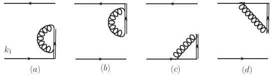
Figure 1: The one-loop diagrams of the wave function.The double line represents the gauge link in Eq.(7).

2. To determine the hard part at one-loop, one needs to calculate the form factor and wave functions with the quark pairs at one-loop. With these one-loop results and by expanding the right-hand side of Eq.(1) in $\alpha_{s}$ one can obtain $H^{(1)}$. $H^{(1)}$ will receive a contribution proportional to

$$H^{(0)}\otimes\phi^{(1)}=\int_{0}^{1}dx\int d^{2}k_{\perp}H^{(0)}(x,k_{\perp},y_{0},k_{2\perp})\phi^{(1)}(x,k_{\perp}),$$ (6)

where $\phi^{(1)}$ is the one-loop contribution to $\phi$ calculated with the off-shell quark pair. The wave function $\phi$ of the incoming $\pi(P)$ is defined as:

$$\phi(x,k_{T},\zeta,\mu)=\int\frac{dz^{-}d^{2}z_{\perp}}{(2\pi)^{3}}e^{ixP^{+}z^{-}-i\vec{z}_{\perp}\cdot\vec{k}_{T}}\langle 0|\bar{q}(0)L_{u}^{\dagger}(\infty,0)\gamma^{+}\gamma_{5}L_{u}(\infty,z)q(z)|\pi(P)\rangle\biggr{|}_{z^{+}=0},$$ (7)

where $L_{u}(\infty,z)$ is a gauge link starting from the space-time point $z$ to $\infty$ along the vector $u$. The vector $u$ is defined as $u^{\mu}=(u^{+},u^{-},0,0)$. In the above definition the limit $u^{+}\rightarrow 0$ should be taken, i.e., any term proportional $u^{+}$ should be neglected. The limit is taken after all loop-integrations. Besides $x$, $k_{T}$ and the renormalization scale $\mu$ the wave function depends on the vector $u$ through the parameter $\zeta^{2}=2u^{-}(P^{+})^{2}/u^{+}\approx(2u\cdot P)^{2}/u^{2}$. This results in that the hard part $H$ will also depend on $\zeta$. This $\zeta$-dependence is very useful for resummation of double log’s.

Similarly, one can defined the wave function of the outgoing $\pi(K)$ with the gauge link along the direction $u^{\prime\mu}=(u^{\prime+},u^{\prime-},0,0)$ in the limit $u^{\prime-}\rightarrow 0$. The wave function of $\pi(K)$ and hence the hard part will also depend on $\zeta^{\prime}$, defined as $\zeta^{\prime 2}=2u^{\prime+}(K^{-})^{2}/u^{\prime-}\approx(2u^{\prime}\cdot K)^{2}/u^{\prime 2}$. Therefore, the two wave functions are in general different. In practice one may take the choice $\zeta=\zeta^{\prime}$. Our discussion in the following will not be affected if one makes or does not make the choice.

The wave function has been studied with an on-shell quark pair at one-loop in [7]. The obtained results are gauge-invariant. But, the wave function in the $k_{T}$-factorization is calculated with an off-shell quark pair, it is not gauge-invariant. Hence, it is possible that the $\zeta$-dependence is also gauge-dependent. This in turn gives to the hard part $H$ a gauge-dependent $\zeta$-dependence, since the form factor does not depend on $\zeta$. If this is the case, it clearly indicates the gauge-variance of the $k_{T}$-factorization. In the general covariant gauge, because the gauge-dependent term in Eq.(4) is proportional to $q^{\mu}q^{\nu}$, it is very simple to show that this term does not give at one-loop the $\zeta$-dependence extra than that in Feynman gauge. However, it is unclear if there exists a gauge-dependent $\zeta$-dependence beyond one-loop. The situation changes if we work with an axial gauge, there is an extra $\zeta$-dependence at one-loop. It is even worse that the extra $\zeta$-dependence is I.R. divergent.

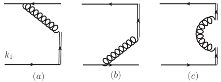
Figure 2: The one-loop diagrams of the wave function. The double line represents the gauge link in Eq.(7).

We take the axial gauge to examine this. The gauge is fixed by $v\cdot G=0$ with the vector $v^{\mu}=(v^{+},v^{-},0,0)$. $v^{+}$ and $v^{-}$ are arbitrary. In the gauge the gluon propagator is given by:

$$\frac{-i}{q^{2}+i\varepsilon}\left[g^{\mu\nu}-\frac{v^{\mu}q^{\nu}+v^{\nu}q^{\mu}}{v\cdot q}+v^{2}\frac{q^{\mu}q^{\nu}}{(v\cdot q)^{2}}\right].$$ (8)

At one-loop, the wave function calculated with the off-shell quark pair is linearly related to the gluon propagator because only one gluon is exchanged. Therefore, the possible extra $\zeta$-dependence can only come from the second term in the above. The possible contributions to this are represented by diagrams given in Fig.1 and Fig.2. We denote the one-loop contribution from the second term to the wave function as $\phi^{(1)}_{v}$. The calculations are simple, e.g., the contribution from Fig.1c:

$$\phi^{(1)}_{v}\biggr{|}_{1c}=-ig_{s}^{2}\delta(x-x_{0})\delta^{2}(\vec{k}_{T}-\vec{k}_{1\perp})C_{F}\int\frac{d^{4}q}{(2\pi)^{4}}\frac{u\cdot v{\rm Tr}\left(\gamma^{-}\gamma_{5}\gamma^{+}\gamma_{5}\gamma\cdot(k_{1}-q)\gamma\cdot q\right)}{(u\cdot q-i\varepsilon)(q^{2}+i\varepsilon)((k_{1}-q)^{2}+i\varepsilon)(v\cdot q)},$$ (9)

where we used for the external lines of the off-shell quark pair the spin projection discussed before. For the gluon propagator in Fig.1c we only used a part in the second term in Eq.(8). Only this part deliveries the extra $\zeta$-dependence. A caution should be taken for the denominator $1/v\cdot q$ in the above when one integrates over $q^{-}$. One needs to supply a prescription for the denominator. This can give in the integration an additional pole than the pole from the first term. But the contribution from the additional pole does not depend on $\zeta$ in the limit $\zeta\rightarrow\infty$. In principle there should be a transverse gauge link at $z^{-}=\infty$ in Eq.(7) to make the definition completely gauge invariant. In our case as long as we keep $u^{+}$ and $v^{+}$ nonzero, the transverse gauge link will not introduce any contribution.

It is straightforward to perform the loop integral in Eq.(9) and other loop integrals in Fig.1. In the calculation we will meet possible I.R. divergences. We introduce a small mass $\lambda$ for gluons to regularize the I.R. divergences. We have from Fig.1:

$$\zeta\frac{\partial}{\partial\zeta}\phi^{(1)}_{v}(x,k_{T},\zeta,\mu)\biggr{|}_{1a} = \zeta\frac{\partial}{\partial\zeta}\phi^{(1)}_{v}(x,k_{T},\zeta,\mu)\biggr{|}_{1b}=\phi^{(0)}(x,k_{T},\zeta,\mu)\frac{\alpha_{s}C_{F}}{2\pi}\ln\frac{\lambda^{2}}{\mu^{2}},$$

$$\zeta\frac{\partial}{\partial\zeta}\phi^{(1)}_{v}(x,k_{T},\zeta,\mu)\biggr{|}_{1c} = -\phi^{(0)}(x,k_{T},\zeta,\mu)\frac{\alpha_{s}C_{F}}{\pi}\left[\ln\frac{\zeta^{2}x^{2}}{k^{2}_{T}}+\frac{1}{2}\ln\frac{\zeta^{2}x^{2}}{\mu^{2}}\right],$$

$$\zeta\frac{\partial}{\partial\zeta}\phi^{(1)}_{v}(x,k_{T},\zeta,\mu)\biggr{|}_{1d} = -\phi^{(0)}(x,k_{T},\zeta,\mu)\frac{\alpha_{s}C_{F}}{\pi}\left[\ln\frac{\zeta^{2}(1-x)^{2}}{k^{2}_{T}}+\frac{1}{2}\ln\frac{\zeta^{2}(1-x)^{2}}{\mu^{2}}\right],$$ (10)

For the contributions from Fig.2 it is easy to show that the sum does not depend on $\zeta$:

$$\zeta\frac{\partial}{\partial\zeta}\left[\phi^{(1)}_{v}(x,k_{T},\zeta,\mu)\biggr{|}_{2a}+\phi^{(1)}_{v}(x,k_{T},\zeta,\mu)\biggr{|}_{2b}+\phi^{(1)}_{v}(x,k_{T},\zeta,\mu)\biggr{|}_{2c}\right]=0.$$ (11)

Therefore we have in the gauge $v\cdot G=0$ for the wave function and the hard part $H$ at one-loop:

$$\zeta\frac{\partial}{\partial\zeta}\phi(x,k_{T},\zeta,\mu) = \left[V\otimes\phi\right]+\frac{\alpha_{s}C_{F}}{2\pi}\left[2\ln\frac{\lambda^{2}}{k_{T}^{2}}-3\ln\frac{\zeta^{2}x^{2}}{k^{2}_{T}}-3\ln\frac{\zeta^{2}(1-x)^{2}}{k^{2}_{T}}\right]\phi(x,k_{T},\zeta,\mu),$$

$$\zeta\frac{\partial}{\partial\zeta}H(x,k_{T},\zeta) = -\left[V\otimes H\right]-\frac{\alpha_{s}C_{F}}{2\pi}\left[2\ln\frac{\lambda^{2}}{k_{T}^{2}}-3\ln\frac{\zeta^{2}x^{2}}{k^{2}_{T}}-3\ln\frac{\zeta^{2}(1-x)^{2}}{k^{2}_{T}}\right]H(x,k_{T},\zeta),$$ (12)

where we use the notation $V\otimes\phi$ and $V\otimes H$ to denote the contributions from Feynman gauge, i.e., the contributions from the first term in Eq.(8). The difference of signs in the two evolutions reflects the fact that the form factor does not depend on $\zeta$. From the above results, it is clear that the hard part $H$, hence the $k_{T}$-factorization, is gauge-dependent, because it is different in different gauges. In the axial gauge, the extra $\zeta$-dependence is I.R. divergent because of the contributions from Fig.1a and 1b. Since the hard part receives the $\zeta$-dependence only from the wave function, the hard part in fact contains a $\zeta$-dependent I.R. divergence. This leads to the conclusion that the factorization is violated in this gauge.

3. In the general covariant gauge the hard part will receive a soft divergence called light-cone divergence, as shown in [2]. In [3] a method to eliminate this divergence is suggested. But, this method is inconsistent as pointed out in [4]. Here, we explain the inconsistence in detail.

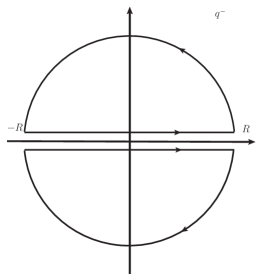
Figure 3: The contours for the integration of $q^{-}$.

The gauge-dependent contributions at one-loop are proportional to $\alpha$ in Eq.(4). We denote these contributions as $\phi_{\alpha}$. We take Fig.2b as an example. The gauge-dependent part is[2, 3]:

$$\phi_{\alpha}(x,k_{T})\biggr{|}_{2b}=\frac{8i\alpha\alpha_{s}}{\pi^{2}}\int_{-\infty}^{\infty}\frac{dq^{-}}{2\pi}\frac{2(k_{1}^{+}-q^{+})q^{-}-\vec{k}_{1\perp}\cdot\vec{q}_{\perp}+q_{\perp}^{2}}{[(k_{1}-q)^{2}+i\varepsilon](q^{2}+i\varepsilon)^{2}}\;.$$ (13)

In the above $q$ is the momentum carried by the gluon in Fig.2b. The components $q^{+}$ and $q_{\perp}^{\mu}$ are fixed as $q^{+}=k_{1}^{+}-xP^{+}$ and $\vec{q}_{\perp}=\vec{k}_{1\perp}-\vec{k}_{T}$ with $k_{1}^{+}=x_{0}P^{+}$. The integral can simply be calculated by taking a closed contour in the upper-half- or in the lower-half complex plan of $q^{-}$, as showing in Fig.3, where we take the contours consisting of a straight line along the real axis and a semi circle with the radius $R$. The limit $R\rightarrow\infty$ should be taken corresponding to that the integration over $q^{-}$ is from $-\infty$ to $\infty$. From positions of $q^{-}$-poles of the integrand the integral only becomes nonzero in the region $0\leq q^{+}\leq x_{0}P^{+}$, because in this region, the pole from the $1/[(k_{1}-q)^{2}+i\varepsilon]$ is in the upper-half plan and the double pole from $1/(q^{2}+i\varepsilon)^{2}$ is in the lower-half plan. For the region $q^{+}<0$ all poles are above the real axis, while all pole are below the real axis for $q^{+}>x_{0}P^{+}$. Taking any one of the two contours the integral can be performed. The result does not depend on the choice of contours.

It is found in [2] that the result is singular. To clearly see this, we take a test function $t(x,k_{\perp})$ to calculate the convolution $t\otimes\phi^{(1)}$. By taking $t(x,k_{\perp})=H^{(0)}(x,k_{\perp},y_{0},k_{2\perp})$ one obtains the convolution in Eq.(6). The singularity can be regularized by a small gluon mass $\lambda_{L}$ or with dimensional regularization as showing in [8]. We first discuss the case with the dimensional regularization, in which the transverse space is $2-\epsilon_{L}$ dimensional with $\epsilon_{L}\rightarrow 0$. We have then the singular contribution of $\phi_{\alpha}|_{2b}$ and the convolution:

$$\phi_{\alpha}\biggr{|}_{2b} = -\frac{4\alpha\alpha_{s}}{\pi^{2}}\frac{k^{2}_{1\perp}\theta(q^{+})\theta(k_{1}^{+}-q^{+})}{k_{1}^{+}(q^{2}_{\perp}+q^{+}k^{2}_{1\perp}/k_{1}^{+})^{2}}+{\rm finite\ terms},$$

$$t\otimes\phi_{\alpha}\biggr{|}_{2b} = \frac{8\alpha\alpha_{s}}{\pi P^{+}}t(x_{0},k_{1\perp})\left(\frac{1}{\epsilon_{L}}\right)+({\rm finite\ terms}).$$ (14)

From Eq.(13) it is clear that the singularity comes from the momentum region where $q$ has the scaling patten $q^{\mu}\sim(\delta_{0}^{2},1,\delta_{0},\delta_{0})$ with $\delta_{0}\ll 1$. The singularity comes from the first term in Eq.(13). We call this as light-cone singularity. Adding all contributions at one-loop the singularity is not canceled. It results in that the hard part $H$ at one-loop is divergent in the general covariant gauge. It should be noted that the form factor does not contain such singularities[2, 9].

To deal the singularity a method is suggested in [3]. In the method one keeps $R$ large but finite in the calculation of the wave function and the limit $R\rightarrow\infty$ is only taken after that the integrals in the convolution are performed. Then one obtains for the wave function not only the contribution from the pole but also the contribution from the semi-circle. As suggested in [3] for the contribution from Fig.2b, one takes the contour for $0<q^{+}$ in the upper-half plan and the contour for $q^{+}<0$ in the lower half plan, one then has:

$$\phi_{\alpha}\biggr{|}_{2b} = -\frac{4\alpha\alpha_{s}}{\pi^{2}}\frac{k^{2}_{1\perp}\theta(q^{+})\theta(k_{1}^{+}-q^{+})}{k_{1}^{+}(q^{2}_{\perp}+q^{+}k^{2}_{1\perp}/k_{1}^{+})^{2}}-\frac{4\alpha\alpha_{s}}{\pi^{3}}\left[\theta(q^{+})\int_{\pi}^{0}d\theta+\theta(-q^{+})\int_{-\pi}^{0}d\theta\right]{\mathcal{F}}_{R}(\theta,x,k_{\perp})+\cdots,$$ (15)

$${\mathcal{F}}_{R}(\theta,x,k_{\perp})=\frac{2(k_{1}^{+}-q^{+})(Re^{i\theta})^{2}}{(2q^{+}Re^{i\theta}-q_{\perp}^{2})^{2}[2(q^{+}-k_{1}^{+})Re^{i\theta}-|{\vec{k}}_{1\perp}-{\vec{q}}_{\perp}|^{2}]},$$

where ${\mathcal{F}}_{R}$ is the first term in Eq.(12) with $q^{-}=Re^{i\theta}$. There are finite terms denoted as $\cdots$. The terms in the second line are from semi circles. If we take the limit $R\rightarrow\infty$ in the above as required in Eq.(13), we obtain the result in Eq.(14). This also results in that $\phi_{\alpha}|_{2b}$ is nonzero only in the region $0<q^{+}<k_{1}^{+}$ or $0<x<x_{0}$. As suggested in [3] one should keep $R$ finite here and calculate the convolution first. The limit is taken after the integrations in the convolution. In this case one has:

$$t\otimes\phi_{\alpha}\biggr{|}_{2b} = \frac{8\alpha\alpha_{s}}{\pi P^{+}}t(x_{0},k_{1\perp})\left(\frac{1}{\epsilon_{L}}\right)+\cdots$$ (16)

$$-\frac{4\alpha\alpha_{s}}{\pi^{3}P^{+}}\lim_{R\rightarrow\infty}\int d^{2}q_{\perp}\left[\int_{\pi}^{0}d\theta\int_{0}^{k_{1}^{+}}dq^{+}+\int_{-\pi}^{0}d\theta\int_{-\infty}^{0}dq^{+}\right]t(x,k_{\perp}){\mathcal{F}}_{R}(\theta,x,k_{\perp}),$$

Working out the singular part of the integrals in the second line and taking the limit $R\rightarrow\infty$ one has:

$$t\otimes\phi_{\alpha}\biggr{|}_{2b}=\frac{8\alpha\alpha_{s}}{\pi P^{+}}t(x_{0},k_{1\perp})\left(\frac{1}{\epsilon_{L}}\right)+\frac{4\alpha\alpha_{s}}{P^{+}\pi^{2}}\left[\int_{\pi}^{0}d\theta-\int_{-\pi}^{0}d\theta\right]t(x_{0},k_{1\perp})\left(\frac{1}{\epsilon_{L}}\right)+({\rm finite\ terms}).$$ (17)

From the above the convolution calculated with the method from [3] is free from the singularity. Two observations can be made at the first look from the above result. Because the limit $R\rightarrow\infty$ is taken after the integrals in the convolution, it implies that one introduces a cut-off for $q^{-}$ with $|q^{-}|<R$. It is unclear how to implement the cut-off in the definition in Eq.(7). The finite $R$ results in that the contribution is not zero with $q^{+}<0$ corresponding to $x>x_{0}$. Another observation is that the result depends on contours. Different choices of contours give different results.

For the region with $0<q^{+}$ or $q^{+}<0$ one always has two possibilities of contours, respectively. In the above the contour for $0<q^{+}$ is in the upper-half plan. If we take the contour in the lower-half plan with the finite $R$ for $0<q^{+}$ and $0>q^{+}$, we then have:

$$\phi_{\alpha}\biggr{|}_{2b}=-\frac{4\alpha\alpha_{s}}{\pi^{2}}\frac{k^{2}_{1\perp}\theta(q^{+}-q_{0}^{+})\theta(k_{1}^{+}-q^{+})}{k_{1}^{+}(q^{2}_{\perp}+q^{+}k^{2}_{1\perp}/k_{1}^{+})^{2}}-\frac{4\alpha\alpha_{s}}{\pi^{3}}\left[\theta(q^{+})\int_{-\pi}^{0}d\theta+\theta(-q^{+})\int_{-\pi}^{0}d\theta\right]{\mathcal{F}}_{R}(\theta,x,k_{\perp})+\cdots,$$ (18)

where $q_{0}^{+}=q^{2}_{\perp}/(2R)$. Here the contribution from the double pole starts at $q^{+}=q_{0}^{+}$ instead of $q^{+}=0$, because the double pole with small enough $q^{+}$ can be in the outside of the contour with $R$. In the above the first $\theta$-integral is from $\theta=-\pi$ to $\theta=0$ because the contour here is in the lower-half plan. Comparing with Eq.(15), one realizes that $\phi_{\alpha}|_{2b}$ is different with different contours. This in turn gives different results of the convolution.

Analyzing all possibilities one can have three different results for the following choices of contours in the two regions of $q^{+}$: (I). All contours are in the upper-half plan or in the lower-half plan. (II). The contour for $0<q^{+}$ is in the upper-half plane and the contour for $q^{+}<0$ is in the lower-half plan. (III). The contour for $0<q^{+}$ is in the lower-half plane and the contour for $q^{+}<0$ is in the upper-half plan. The choice (II) corresponding to Eq.(15,16). The different results for these 3 choices are summarized as:

$$t\otimes\phi_{\alpha}\biggr{|}_{2b} = \frac{8\alpha\alpha_{s}}{\pi P^{+}}t(x_{0},k_{1\perp})\left(\frac{1}{\epsilon_{L}}\right)+({\rm finite\ terms}),\ \ \ {\rm for\ (I)},$$

$$t\otimes\phi_{\alpha}\biggr{|}_{2b} = \frac{8\alpha\alpha_{s}}{\pi P^{+}}t(x_{0},k_{1\perp})\left(\frac{1}{\epsilon_{L}}\right)-\frac{8\alpha\alpha_{s}}{\pi P^{+}}t(x_{0},k_{1\perp})\left(\frac{1}{\epsilon_{L}}\right)+({\rm finite\ terms}),\ \ \ {\rm for\ (II)},$$

$$t\otimes\phi_{\alpha}\biggr{|}_{2b} = \frac{8\alpha\alpha_{s}}{\pi P^{+}}t(x_{0},k_{1\perp})\left(\frac{1}{\epsilon_{L}}\right)+\frac{8\alpha\alpha_{s}}{\pi P^{+}}t(x_{0},k_{1\perp})\left(\frac{1}{\epsilon_{L}}\right)+({\rm finite\ terms}),\ \ \ {\rm for\ (III)}.$$ (19)

This is the contour dependence pointed out in [4]. The cancelation of the singularity depends on the choice of contours with the method in [3].

One may use a small gluon mass $\lambda$ to regularize the singularity. The mass in the general covariant gauge is introduced as in [10]:

$$\frac{-ig^{\mu\nu}}{q^{2}-\lambda^{2}+i\varepsilon}+i\alpha\frac{q^{\mu}q^{\nu}}{(q^{2}-(1-\alpha)\lambda^{2}+i\varepsilon)(q^{2}-\lambda^{2}+i\varepsilon)}.$$ (20)

Comparing with Eq.(4), the double pole in the $q^{-}$-plan splits into two single poles. It can be shown with the method in [3] that the singularity is canceled by the contributions from semi circles. It is interesting to note that the cancelation is contour-independent, because an additional contribution from the cases where one of the two single poles can be in the outside of a closed contour with the finite $R$. However, this only works at one-loop, because one has at one-loop only diagrams similar to QED. Beyond one-loop level, one can not take a finite gluon mass here for QCD.

A natural question with the suggest method in [3] is then which answer is correct? When one takes the dimensional regularization, the result is contour-dependent. When one uses a finite gluon mass for the regularization, it is definitely not correct beyond one-loop level. From the above analysis different results about the singularity are due to keeping $R$ finite in Eq.(15) instead of $R\rightarrow\infty$. In fact, none of them is correct in the sense that $R$ can not be kept finite in the wave function. A finite $R$ is in conflict with translational covariance. Below we discuss the conflict in detail.

We start with the well-known fact that the wave function becomes zero with $x>1$. This is derived by sandwiching a complete set of states into Eq.(7) and using the translational covariance. It should be noted that $x_{0}$ in Eq.(2) is arbitrary in the region $0<x_{0}<1$. For nonzero $k_{1\perp}$ we can take $x_{0}=1$ for the off-shell quark pair $q(k_{1})\bar{q}(P-k_{1})$ as an extreme case without any problem, because the quark and the antiquark with $x_{0}=1$ still have nonzero momenta. Then, with a large but still finite $R$, the wave function is not zero with $x>1$. This can also be seen from the contributions in Eq.(15). Therefore, a finite $R$ is in conflict with translational covariance in the case with $x_{0}=1$. In general, as showing in [4], the contributions to the wave function from a class of diagrams including Fig.2b, where gluons are only exchanged between the quark field $q(z)$ and $L_{u}^{\dagger}(\infty,0)$ in Eq.(7) or are exchanged to form self-energy corrections to $q(z)$ and $L_{u}^{\dagger}(\infty,0)$, are proportional to

$$\int\frac{dz^{-}}{2\pi}\frac{d^{2}z_{\perp}}{(2\pi)^{2}}e^{ixP^{+}z^{-}-i\vec{z}_{\perp}\cdot\vec{k}_{T}}\langle 0|\left(L_{u}^{\dagger}(\infty,0)-1\right)\gamma^{+}\gamma_{5}q(z)|q(k_{1})\rangle|_{z^{+}=0}$$ (21)

besides some trivial factors. The leading order result of the above expression is given by Fig.2b by deleting the antiquark line. Sandwiching a complete set of states and using the translational covariance, it is easy to show that the above quantity must be zero with $x>x_{0}$. Here $x_{0}$ is arbitrary in the region $0<x_{0}<1$. Therefore, the contribution from Fig.2b must be zero with $x>x_{0}$. A nonzero contribution from Fig.2b with $x>x_{0}$ is unphysical. Taking $|q^{-}|<R$ instead of $|q^{-}|<\infty$ in Eq.(13,15), it results in that the contribution is not zero with $x>x_{0}$. One also notes from Eq.(15,18) that with the finite $R$ the wave function is not zero for $q^{+}>k_{1}^{+}$ or $x<0$. It implies that the quark entering hard scattering is with a negative energy. This is inconsistent not only with the translational covariance but also with physical picture.

From the above discussion, it is clear that the method of [3] by keeping $R$ finite in the wave function is essentially to include the unphysical contributions. Convoluting the wave function containing these unphysical contributions with a test function, the discussed light-cone singularities may be canceled. The cancelation depends on contours and also on how the singularities are regularized. As shown in the above, the existence of these unphysical contributions is in conflict with general principles, i.e., with the translational covariance. Because of this and the contour dependence the method is not consistent. We emphasize here that the key problem of the method is the inconsistence with the translational covariance for the defined wave function in Eq.(7). This in fact can be easily seen by noting the following fact: The finite cut-off $R$ for $q^{-}$ implies that one takes the corresponding space-time coordinate $x^{+}$ as one-dimensional lattice with the lattice spacing $2\pi/R$. The lattice certainly has no symmetry of translational covariance. The conclusion here is, as made in [2, 4], that the hard part will contain the divergent part in the general covariant gauge. Hence the $k_{T}$-factorization is gauge-dependent and violated in this gauge.

To summarize: With the results presented in this note, one can conclude that the $k_{T}$-factorization is gauge-dependent and violated in the gauges studied here. Since some sources of the gauge dependence studied here are from wave functions and absent in scattering amplitudes of off-shell partons, the $k_{T}$-factorization is gauge-variant for any exclusive process. Our results can be generalized to the case of $B$-meson decays. Therefore, the $k_{T}$-factorization for exclusive $B$-meson decays is also gauge-dependent.

Note added:

After we completed the present work, an analysis of three-parton contribution to the $\pi$-form factor in the $k_{T}$-factorization appeared in [11]. The contribution is at twist-three, where the spin projection for the initial- and final off-shell quark pair are $\sigma^{-\alpha}\gamma_{5}$ and $\sigma^{+\beta}\gamma_{5}$, respectively. In [11] the $k_{T}$-factorization has also been studied in the general covariant gauge. Because the different spin projections, the results obtained in [11] has no implication for our result in Eq.(5) and our discussion there. But the results with the general covariant gauge in [11] clearly show that the factorization is gauge-variant.

From the results in [11] the gauge dependent part in the three-parton contribution related to the initial $\pi$ can be written in the form of the following convolution:

$$\alpha H_{\mu\nu}\otimes\langle 0|\bar{q}(y)\gamma_{5}\gamma^{+}\gamma^{\mu}D^{\nu}(0)q(0)|\pi(P)\rangle,$$ (22)

where $\alpha$ is the gauge parameter in Eq.(4) and $H^{\mu\nu}$ is perturbative coefficient function. The field $\bar{q}$ is with $y^{\mu}=(0,y^{-},\vec{y}_{\perp})$. It should be noted $\vec{y}_{\perp}\neq 0$ because the quark carries a nonzero transverse momentum into hard scattering in the $k_{T}$-factorization. For $\vec{y}_{\perp}=0$ the above matrix-element is of twist-3 in collinear factorization. It has been argued in [11] that the above expression is zero because of the equation of motion. But it is not true. There are two possibilities to have the above quantity to be zero with equation of motion. If one has $H^{\mu\nu}\propto g^{\mu\nu}$, it is clear that the quantity is zero. In general, the perturbative coefficient functions related to the derivative and to the gluon field in the covariant derivative $D^{\nu}(x)=\partial^{\nu}+ig_{s}G^{\nu}(x)$ can be different. In [11] one has shown that the contribution related to the $\partial^{+}$ can be neglected and the attachment of a $+$-component of gluon to the hard scattering diagrams gives no contribution. From these results one has $H^{+-}=0$. Therefore, $H^{\mu\nu}$ is not proportional to $g^{\mu\nu}$. Another possibility is that the matrix element is proportional to $g^{\mu\nu}$. But again this is not correct. To show this, one can make a Fourier transformation of $\langle 0|\bar{q}(y)\gamma_{5}\gamma^{\rho}\gamma^{\mu}D^{\nu}(0)q(0)|\pi(P)\rangle$ and study its decomposition. The decomposition is complicated. The first few terms are:

$$P^{+}\int\frac{dy^{-}d^{2}y_{\perp}}{(2\pi)^{3}}e^{-ixP^{+}y^{-}+i\vec{k}_{\perp}\cdot\vec{y}_{\perp}}\langle 0|\bar{q}(y)\gamma_{5}\gamma^{\rho}\gamma^{\mu}D^{\nu}(0)q(0)|\pi(P)\rangle$$

$$=f_{0}(x,k_{\perp})\left(P^{\rho}g^{\mu\nu}-g^{\rho\nu}P^{\mu}\right)+f_{1}(x,k_{\perp})g^{\rho\mu}P^{\nu}+f_{2}(x,k_{\perp})\left(g^{\rho\nu}k_{\perp}^{\mu}-g^{\mu\nu}k_{\perp}^{\rho}\right)+f_{3}(x,k_{\perp})g^{\rho\mu}k_{\perp}^{\nu}$$

$$\ \ \ +f_{4}(x,k_{\perp})\left(P^{\rho}k_{\perp}^{\mu}k_{\perp}^{\nu}-P^{\mu}k_{\perp}^{\rho}k_{\perp}^{\nu}\right)+\cdots,$$ (23)

where $\cdots$ denote the structures which are zero when $\rho=+$ and those may depend on $n^{\mu}=(0,1,0,0)$. In general the functions $f_{0,1,2,\cdots}$ are not zero. From the reason of dimension they may be at the same level of importance. This can also be seen the constraint of $f$’s obtained by contracting $g_{\mu\nu}$ from both sides. Taking $\rho=+$, one clearly sees that the matrix element is not proportional to $g^{\mu\nu}$. Therefore, the above quantity is not zero. This shows that the three-parton contribution in the $k_{T}$-factorization for the $\pi$-form factor in [11] is gauge-dependent.

Acknowledgments

This work is supported by National Nature Science Foundation of P.R. China(No. 10805028, 10975169, 11021092).

References

• [1] S. Nandi and H.-n. Li, Phys. Rev. D76 (2007) 034008, e-Print: arXiv:0704.3790 [hep-ph].
• [2] F. Feng, J.P. Ma and Q. Wang, Phys. Lett. B674 (2009) 176, e-Print: arXiv:0807.0296 [hep-ph].
• [3] H.-n. Li and S. Mishima, Phys. Lett. B674 (2009) 182, e-Print: arXiv:0808.1526 [hep-ph].
• [4] F. Feng, J.P. Ma and Q. Wang, Phys. Lett. B677 (2009) 121, e-Print: arXiv:0808.4017 [hep-ph].
• [5] H.-n. Li, Y.L. Shen, Y.M. Wang and H. Zou, e-Print: arXiv:1012.4098 [hep-ph].
• [6] Z.T. Wei, private communication.
• [7] J.P. Ma and Q. Wang, Phys. Lett. B642 (2006) 232, hep-ph/0605075.
• [8] F. Feng, J.P. Ma and Q. Wang, e-Print: arXiv:0901.2965 [hep-ph].
• [9] F. Feng, J.P. Ma and Q. Wang, e-Print: arXiv:0808.4017v1 [hep-ph].
• [10] C. Itzykson and J. Zuber, Quantum Field Theory, New York, McGraw-Hill (1980).
• [11] Y.-C. Chen and H.-n. Li, e-Print: arXiv:1104.5398 [hep-ph].