Aharonov-Bohm oscillations in the local density of topological surface states

Abstract

We study Aharonov-Bohm (AB) oscillations in the local density of states (LDOS) for topological insulator (TI) and conventional metal Au(111) surfaces with spin-orbit interaction, which can be probed by spin-polarized scanning tunneling microscopy. We show that the spacial AB oscillatory period in the total LDOS is a flux quantum $\Phi_{0}\mathtt{=}hc/e$ (weak localization) in both systems. Remarkably, an analogous weak antilocalization with $\Phi_{0}/2$ periodic spacial AB oscillations in spin components of LDOS for TI surface is observed, while it is absent in Au(111).

Spin-orbit interaction (SOI) effects in semiconductors and metals have been an active theme in the modern condensed matter physics, but especially, the topological insulators (TI), which have been detected in series of two-dimensional Kane ; Bernevig ; Konig and three-dimensional Fu ; Hsieh1 ; Chen ; Hsieh3 ; Xia ; Moore ; Qi ; Zhanghj materials, suggest new directions for this field since the extraordinarily strong SOI exists in TI. The helical spin structure of electrons in TI acquire a spin-orbit induced nontrivial Berry phase of $\pi$ after a $2\pi$ adiabatic rotation along the Fermi surface. This Berry phase corrects the quantum constructive interference between a closed trajectory that the electron passes and its time-reversal counterpart, and thus can give rise to the weak antilocalization (WAL) signature in the quantum coherent magneto-transport coefficients. Many efforts have been devoted to observing WAL in the HgTe quantum wells Olshanetsky ; Tkachov , Bi₂Te₃ Hasan ; He ; Ghaemi , Bi₂Se₃ Peng ; Bardarson ; ZhangY ; Chen2 ; Checkelsky ; Liu ; Wang , and other materials. Very recently, for example, in a transport experiment Peng of Bi₂Se₃ nanowires, the Aharonov–Bohm (AB) oscillation with anomalous period $\Phi_{0}\mathtt{=}hc/e$ (twice the conventional period) of magnetoconductance was observed, while the WAL induced $\Phi_{0}/2$ period was absent. The period of these oscillations in conductance is determined by the doping level and the disorder of the TI nanowire Bardarson ; ZhangY . In addition, an energy gap at the Dirac cone opened by magnetic doping in TI films could also induce crossover from the WAL to the weak localization (WL), which is tunable by the Fermi energy and the gap Lu .

In this letter, for exploring the analogous WAL in topological surface state, we consider an imaginary AB interferometer consisting of a spin-polarized scanning tunneling microscope (SP-STM) tip Meier ; Bergmann1 ; Schmaus and two identical nonmagnetic impurities apart tens of nanometers on the TI surface as shown in Fig. 1. When an electron travels along the clockwise and anticlockwise loops ($\mathbf{r}\mathtt{\rightleftharpoons}\mathbf{r}_{1}\mathtt{\rightleftharpoons}\mathbf{r}_{2}\mathtt{\rightleftharpoons}\mathbf{r}$) enclosing a finite area, the quantum interference phenomenon occurs. The interference contribution to the local density of states (LDOS) is affected by an external magnetic field $B$ via the AB effect arising from the threaded magnetic flux Cano . We will show that, on one hand, the AB oscillatory period of the total LDOS $\Delta N_{L}\left(\mathbf{r}\mathtt{,}\omega\mathtt{,}B\right)$ (the subscription $L$ represents the loops enclosed by the scattering paths of the surface electrons) is a flux quantum $\Phi_{0}$, which is an analog of WL phenomenon. On the other hand, the strong SOI in TI materials can modify the electron AB interference effect via the chiral spin rotations during the non-collinear multiple scattering processes, and thereby the analogous WAL effect with $\Phi_{0}/2$ period in AB oscillations will be observed if the spin-resolved LDOS [$\Delta N_{L}^{\uparrow}\left(\mathbf{r}\mathtt{,}\omega\mathtt{,}B\right)$ and $\Delta N_{L}^{\downarrow}\left(\mathbf{r}\mathtt{,}\omega\mathtt{,}B\right)$] are measured. Furthermore, for comparison, we briefly discuss the AB effect in the LDOS of conventional metal Au(111) surface with weak SOI, and find that the analogous WAL phenomenon is absent in Au(111) surface. Our finding may provide a useful method to characterize the topological surface states.

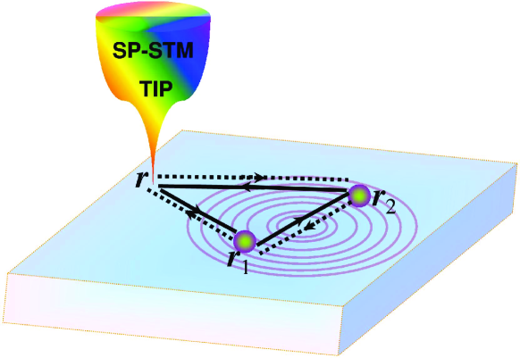
Figure 1: (Color online) Surface electronic interferometer, comprising a spin polarized STM tip at $\mathbf{r}$ and two impurities at $\mathbf{r}_{1}$ and $\mathbf{r}_{2}$ separately. The interference contributions in the LDOS is introduced by the electrons traveling along clockwise and anticlockwise loops enclosed by the STM tip and two impurities. The applied magnetic field affects this interference via the AB effect.

We describe the TI surface, on which two nonmagnetic impurities are adsorbed, by a low-energy effective Dirac Hamiltonian written as

$$H=v\boldsymbol{\sigma}\cdot\left(\hat{z}\times\mathbf{q}\right)+V\left(\mathbf{r}\right)$$ (1)

with the Fermi velocity $v\mathtt{=}333$ (287) meV$\cdot$nm in Bi₂Se₃ (Bi₂Te₃) Liu3 . $\mathbf{q}\mathtt{=}\left(q_{x}\mathtt{,}q_{y}\right)$ denotes the planar momentum operator, and $\boldsymbol{\sigma}\mathtt{=}\left(\sigma_{1}\mathtt{,}\sigma_{2}\mathtt{,}\sigma_{3}\right)$ is the Pauli spin matrix. $V$($\mathbf{r}$)$\mathtt{=}\sum_{i\mathtt{=}1}^{2}U_{i}\sigma_{0}\delta\left(\mathbf{r}\mathtt{-}\mathbf{r}_{i}\right)$ is the potential of two nonmagnetic impurities located at $\mathbf{r}_{1}\mathtt{=}\left(\mathtt{-}d/2\mathtt{,}0\right)$ and $\mathbf{r}_{2}\mathtt{=}\left(d/2\mathtt{,}0\right)$ with strength $U_{i}$. $\sigma_{0}$ is the $2\mathtt{\times}2$ unit matrix.

The features we discuss are expected to be seen in the change of the real-space LDOS owing to the influence of magnetic flux which passes through the area enclosed by the two scattering paths shown in Fig. 1. This quantity can directly reveal the WL or WAL effect in TI via AB oscillatory periods in LDOS. The real-space Green’s function involving the impurities scattering is given by Dyson equation $G\mathtt{=}G_{0}\mathtt{+}\delta G$, with

$$\delta G=\int d\mathbf{r}^{\prime\prime}G_{0}\left(\mathbf{r}-\mathbf{r}^{\prime\prime};\omega\right)V\left(\mathbf{r}^{\prime\prime}\right)G\left(\mathbf{r}^{\prime\prime},\mathbf{r}^{\prime};\omega\right).$$ (2)

The bare electron Green’s function $G_{0}\mathbf{\ }$for the TI surface states could be expressed in terms of a complex amplitude multiplied by a “complex” spin rotation:

$$G_{0}\left(\mathbf{r,r}^{\prime};\omega\right)=\frac{\left|\omega^{+}\right|}{4v^{2}}D_{+}\hat{R}\left(\alpha,\beta,\eta\right),$$ (3)

which is useful to gain more physical insight into the transport between $\mathbf{r}$ and $\mathbf{r}^{\prime}$. Here, $D_{+}\mathtt{=}\sqrt{g_{0}^{2}+g_{1}^{2}}$, where $g_{0/1}\mathtt{=}\mathtt{sgn}\left(\omega^{+}\right)Y_{0/1}\left(\left|k\right|\rho\right)\mathtt{\mp}iJ_{0/1}\left(\left|k\right|\rho\right)$ with $\rho\mathtt{=}\left|\mathbf{r}\mathtt{-}\mathbf{r}^{\prime}\right|$, $k\mathtt{=}k_{F}\left(1\mathtt{+}\omega/E_{F}\right)$, $\omega^{+}\mathtt{=}\omega\mathtt{+}E_{F}$, and $E_{F}\mathtt{=}vk_{F}$ the Fermi energy of TI. $J_{0/1}$ ($Y_{0/1}$) are the first (second) kind Bessel functions. $\hat{R}\left(\alpha,\beta,\eta\right)\mathtt{=}e^{i\alpha\sigma_{3}}e^{i\beta\sigma_{1}}e^{i\eta\sigma_{3}}$ is a spin rotation operator characterized by the three Euler angles $\alpha\mathtt{=}\mathtt{-}\frac{\vartheta}{2}\mathtt{+}\frac{\pi}{4}$ with $e^{i\vartheta}\mathtt{=}(\boldsymbol{\rho}\mathtt{\cdot}\hat{x}\mathtt{+}i\boldsymbol{\rho}\mathtt{\cdot}\hat{y})/\rho$, $\beta\mathtt{=}\tan^{-1}\mathtt{(}\frac{g_{1}}{g_{0}}\mathtt{)}$, and $\eta\mathtt{=}\mathtt{-}\alpha$. Equation (3) is exact under a high-energy cutoff Liu2009 ; Biswas2 .

Following the perturbation approach, Eq. (2) can be expanded to any order in the impurity potential $U_{i}$. Our effort will be concentrated on the scattering processes of surface electrons with the both impurities, in which the scattering paths enclose loops. Therefore, taking all this into account, after a long algebra calculation, we have

$$\delta G_{L} =G_{0}\left(\mathbf{r}-\mathbf{r}_{1}\right)W_{1}G_{0}\left(\mathbf{r}_{1}-\mathbf{r}_{2}\right)T_{2}G_{0}\left(\mathbf{r}_{2}-\mathbf{r}^{\prime}\right)$$

$$+G_{0}\left(\mathbf{r}-\mathbf{r}_{2}\right)W_{2}G_{0}\left(\mathbf{r}_{2}-\mathbf{r}_{1}\right)T_{1}G_{0}\left(\mathbf{r}_{1}-\mathbf{r}^{\prime}\right),$$ (4)

where

$$W_{1/2}=\frac{T_{1/2}}{\sigma_{0}-T_{1/2}G_{0}\left(\mathbf{r}_{1/2}-\mathbf{r}_{2/1}\right)T_{2/1}G_{0}\left(\mathbf{r}_{2/1}-\mathbf{r}_{1/2}\right)}$$ (5)

is diagonal with $T\mathtt{-}$matrices $T_{1/2}\mathtt{=}\frac{U_{1/2}}{\mathbf{I}\mathtt{-}U_{1/2}G_{0}\left(\mathbf{0}\mathtt{;}\omega\right)}$. Equation (4) is a general formula describing the interference effect from the scattering with both two impurities participated. In the absence of SOI, the two terms in Eq. (4), i.e., the scattering amplitudes corresponding to the time-reversal processes, should be equal to each other and thereby give rise to the constructive quantum correction to the LDOS in the so-called WL theory. In the presence of a strong SOI, however, the electrons interference is affected remarkably due to the non-collinear multiple scattering trajectories that generate nontrivial spin rotations. The spin rotation leads to a destructive interference in LDOS by a phase change picked up during the clockwise and anticlockwise scattering processes, which is the origin of the WAL effect in systems with strong SOI. Explicitly, for collinear scattering paths between $\mathbf{r}_{1}$ and $\mathbf{r}_{2}$, there is no net spin rotation since $G_{0}\left(\mathbf{r}_{1/2}\mathtt{-}\mathbf{r}_{2/1}\right)G_{0}\left(\mathbf{r}_{2/1}\mathtt{-}\mathbf{r}_{1/2}\right)\mathtt{\varpropto}\sigma_{0}$. Whereas for non-collinear multiple scattering trajectories, such as the loops shown in Fig. 1, $G_{0}\left(\mathbf{r}\mathtt{-}\mathbf{r}_{1/2}\right)G_{0}\left(\mathbf{r}_{1/2}\mathtt{-}\mathbf{r}_{2/1}\right)G_{0}\left(\mathbf{r}_{2/1}\mathtt{-}\mathbf{r}\right)$ is not a unit matrix which implies net spin rotations during scattering processes. As a result, in contrast to the collinear scattering process, the non-collinear multiple-impurity scattering on TI surface can induce dramatic modulations in the LDOS.

Applying a magnetic field tends to destroy the destructive interference and may bring forth some key signatures of WAL effect, such as the $\Phi_{0}/2$ periodic AB oscillations in the spin components of LDOS (similar to $\Phi_{0}/2$ oscillations in the magneto-conductance due to WAL). In the presence of a low magnetic field, the Green’s function can be semiclassically approximated as Altshuler ,

$$\tilde{G}_{0}\left(\mathbf{r}-\mathbf{r}^{\prime}\right)=e^{i\frac{2\pi}{\Phi_{0}}\int_{\mathbf{r}}^{\mathbf{r}^{\prime}}\mathbf{A}\left(\mathbf{l}\right)\cdot d\mathbf{l}}G_{0}\left(\mathbf{r}-\mathbf{r}^{\prime}\right),$$ (6)

where $\mathbf{A}\mathtt{=}\left(\mathtt{-}By\mathtt{,}0\mathtt{,}0\right)$ represents the vector potential. This approximation is exact so long as the magnetic length is much greater than the Fermi wave length [$l_{B}\mathtt{=}\left(\Phi_{0}/2\pi B\right)^{1/2}\mathtt{\gg}\lambda_{F}$]. For magnetic field $B\mathtt{=}5\mathtt{\sim}10$ T, the corresponding magnetic length $l_{B}\mathtt{\approx}11.63\mathtt{\sim}8.22$ nm, while the Fermi wave length $\lambda_{F}\mathtt{=}7.21\mathtt{\sim}5.3$ nm for TI with $E_{F}\mathtt{=}250\mathtt{\sim}340$ meV Chen . Accordingly, the condition in Eq. (6) for the semiclassical approximation is valid for these low magnetic field and low energy ranges. Also, the Zeeman splitting is negligibly small (typically of 1.0 meV at $B\mathtt{=}10$ T for Bi₂Se₃ film) compared to the strong SOI, and thus is not taken into account in the following discussion.

The correction of the LDOS due to the magnetic flux is given by

$$\Delta N_{L}\left(\mathbf{r},\omega,B\right)=-\frac{1}{\pi}\Im\text{Tr}\left[\delta\tilde{G}_{L}\left(\mathbf{r},\omega\right)-\delta G_{L}\left(\mathbf{r},\omega\right)\right],$$ (7)

where $\delta\tilde{G}_{L}$ is calculated from Eq. (4) with $\tilde{G}_{0}$. For large distances ($\left|k\right|\rho\mathtt{\gg}1$), $J_{0/1}\mathtt{\approx}\mathtt{\pm}\sqrt{2/\left(\pi\left|k\right|\rho\right)}\cos\left[\pi/4\mathtt{\mp}\left|k\right|\rho\right]$ and $Y_{0/1}\mathtt{\approx}\mathtt{\pm}\sqrt{2/\left(\pi\left|k\right|\rho\right)}\sin\left[\left|k\right|\rho\mathtt{\mp}\pi/4\right]$. Combining Eqs. (3-7), we get

$$\Delta N_{L}\left(\mathbf{r},\omega,B\right) =\Delta N_{L}^{\uparrow}\left(\mathbf{r},\omega,B\right)+\Delta N_{L}^{\downarrow}\left(\mathbf{r},\omega,B\right)$$

$$\approx C\Im[\tilde{t}\left(\omega\right)e^{i\left[\chi\left(r\right)-\pi/4\right]}]\left[\cos\left(\frac{2\pi\Phi}{\Phi_{0}}\right)-1\right],$$ (8)

where $C\mathtt{\propto}k^{-3/2}\sqrt{\frac{2}{d\rho_{1}\rho_{2}}}\cos\mathtt{(}\frac{\vartheta_{2}}{2}\mathtt{)}\sin\mathtt{(}\frac{\vartheta_{1}}{2}\mathtt{)}\sin\mathtt{(}\frac{\vartheta_{1}\mathtt{-}\vartheta_{2}}{2}\mathtt{)}$ with $e^{i\vartheta_{1/2}}\mathtt{=}(\boldsymbol{\rho}_{1/2}\mathtt{\cdot}\hat{x}\mathtt{+}i\boldsymbol{\rho}_{1/2}\mathtt{\cdot}\hat{y})/\rho_{1/2}$ and $\boldsymbol{\rho}_{1/2}\mathtt{=}\mathbf{r}\mathtt{-}\mathbf{r}_{1/2}$, $\chi\left(r\right)\mathtt{=}k\left(d\mathtt{+}\rho_{1}\mathtt{+}\rho_{2}\right)$. $\tilde{t}\left(\omega\right)\mathtt{=}\frac{t^{2}\left(\omega\right)}{1\mathtt{-}t^{2}\left(\omega\right)\left[g_{0}^{2}\left(d\right)\mathtt{-}g_{1}^{2}\left(d\right)\right]}$ with $t\left(\omega\right)\mathtt{=}\frac{U}{1\mathtt{-}U\mathtt{\int}\frac{d^{2}q}{\left(2\pi\right)^{2}}\frac{i\omega}{\left(i\omega\right)^{2}\mathtt{-}\left(vq\right)^{2}}}$ is the nonzero element of $T\mathtt{-}$matrix. One can notice that $\left[g_{0}^{2}\left(d\right)\mathtt{-}g_{1}^{2}\left(d\right)\right]$ vanishes within the above asymptotic representation of $J_{0/1}$ and $Y_{0/1}$.

In the present setup, we focus solely on the (spin-resolved) LDOS at $\mathbf{r}\mathtt{=}(x,y)$, which is probed by the STM tip with the same plane coordinates $(x,y)$. Since the STM tip also dually plays as a scatter for the electron’s loop motion, thus, in the presence of a fixed magnetic field $B$, the AB oscillation varies with the tip position along the $y$ direction. Obviously, the AB oscillation signatures result from $\cos\mathtt{(}\frac{2\pi\Phi}{\Phi_{0}}\mathtt{)}\mathtt{-}1\mathtt{=}0$ in Eq. (8), and the spacial oscillation period is $d_{0}\mathtt{=}\frac{2\Phi_{0}}{Bd}$ for fixed $B$ and fixed impurities configuration, corresponding to a $\Phi_{0}$ period in the scale of flux, which gives rise to WL effect in the total LDOS. To observe a complete AB oscillation period in $\Delta N_{L}\left(\mathbf{r}\mathtt{,}\omega\mathtt{,}B\right)$, the magnetic field should satisfy the relation

$$B_{2\pi}\sim 2\Phi_{0}/yd.$$ (9)

Now let us analyze the spin-up and spin-down components of LDOS. The extraordinary SOI in TI affects the surface electron interference due to the non-collinear multiple scattering trajectories that generate nontrivial spin rotations, which can be easily obtained by the rotation operator $\hat{R}\left(\alpha,\beta,\eta\right)$ in the Green’s function $G_{0}$. Explicitly, the AB oscillations of spin components of LDOS are given by

$$\Delta N_{L}^{\uparrow/\downarrow}\left(\mathbf{r},\omega,B\right) \approx\mp C_{s}\operatorname{Im}\left[\tilde{t}(\omega)e^{i\left(\chi\left(r\right)-\frac{\pi}{4}\right)}\right]$$ (10)

$$\times\left[\sin\left(\frac{2\pi\Phi}{\Phi_{0}}\mp\phi\right)\pm\sin\phi\right],$$

where $\phi\mathtt{=}\frac{\vartheta_{1}\mathtt{-}\vartheta_{2}}{2}\mathtt{=}\frac{1}{2}\mathtt{[}\tan^{\mathtt{-}1}(\frac{y}{x\mathtt{+}d/2}\mathtt{)}\mathtt{-}\tan^{\mathtt{-}1}\mathtt{(}\frac{y}{x\mathtt{-}d/2}\mathtt{)]}$ and $C_{s}$=$\frac{C}{2}\sin\phi$. As clearly seen from this equation, comparing to the total LDOS, there occur in the spin-resolved LDOS additional strong SOI induced quantum interference signature. The above equation should be reasonable because of the destructive interference brought about by the spin rotation during clockwise and anticlockwise scattering processes as well as by the magnetic field. This strong spin interference effect deviates the real-space AB oscillations from $d_{0}$ period when a SP-STM tip scans on the TI surface in the presence of a fixed $B$, which is our concentration in the present paper. We can easily find that the spacial AB oscillation period of $\Delta N_{L}^{\uparrow/\downarrow}$ is determined by the factor $F^{\uparrow/\downarrow}\mathtt{=}\sin(\frac{2\pi\Phi}{\Phi_{0}}\mathtt{\mp}\phi)\mathtt{\pm}\sin\phi$. Taking $\Delta N_{L}^{\uparrow}$ as an example (Similar analysis can be done on $\Delta N_{L}^{\downarrow}$) to find the AB period, we consider the roots of $F^{\uparrow}\mathtt{=}0$ as an equation of $y$, which can be rewritten as $F^{\uparrow}\mathtt{=}\sin\phi[\cos(\frac{2\pi\Phi}{\Phi_{0}})\mathtt{-}1]\mathtt{-}\cos\phi\sin(\frac{2\pi\Phi}{\Phi_{0}})\mathtt{=}0$. There are two cases that result in $F^{\uparrow}\mathtt{=}0$: (i) First, it is easy to get that $y_{1}\mathtt{=}\frac{2n\Phi_{0}}{Bd}$ $\left(n\mathtt{=}0,\mathtt{\pm}1,\mathtt{\cdots}\right)$ are the roots of $F^{\uparrow}\mathtt{=}0$; (ii) Second, expanding $F^{\uparrow}$ at point $y_{2}\mathtt{=}\frac{\left(2n\mathtt{+}1\right)\Phi_{0}}{Bd}$, a simple equation for $y$ can be obtained $M(y\mathtt{-}\frac{\left(2n\mathtt{+}1\right)\Phi_{0}}{Bd})\mathtt{-}P\mathtt{=}0$, which gives out other asymptotic roots $y\mathtt{=}\frac{\left(2n\mathtt{+}1\right)\Phi_{0}}{Bd}\mathtt{+}\frac{P}{M}$ ($M$ and $P$ are the expanding coefficients). These roots lie near $y_{2}$ and become better for the limit of small $B$ [see following Figs. 2(b) and 2(c)]. Combining with case (i), the AB oscillation signals for $\Delta N_{L}^{\uparrow}$ occur at $\mathtt{\sim}\frac{n\Phi_{0}}{Bd}$ with a spacial period of $\frac{\Phi_{0}}{Bd}\mathtt{=}\frac{d_{0}}{2}$ (i.e., $\frac{\Phi_{0}}{2}$ in the scale of flux), the half of $\Delta N_{L}$. This half period could be understood as an analog of WAL effect in the spin-polarized LDOS since strong SOI in TI can result in the two-dimensional WAL effect in the magneto-conductance, which can be represented as the AB oscillation phenomenon with period of $\frac{\Phi_{0}}{2}$.

Moreover, the interference signature of LDOS decays by a factor of $\left[d\rho_{1}\rho_{2}\right]^{-1/2}$ in the asymptotic representations, Eqs. (8) and (10). Actually, however, dephasing processes have been observed in transport investigations in Bi₂Se₃ and Bi₂Te₃ films Checkelsky ; Wang ; Liu ; He as well as in AB-effect studies of Bi₂Se₃ nanowires Peng ; Bardarson ; ZhangY . The phase coherence length $l_{\phi}$ of Bi₂Se₃ and Bi₂Te₃ can be as large as hundreds of nanometers, which is tens times of the Fermi wave length. The characteristic distance in our setup must be much smaller than the phase coherence length ($d\mathtt{\leq}l_{\phi}$), so that we choose $d\mathtt{=}20$nm$\mathtt{\ll}l_{\phi}$ without taking into account the dephasing processes in the following numerical calculations.

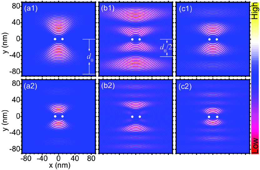
Figure 2: (Color online) Simulations of the AB oscillations of the electronic LDOS in Bi₂Te₃(111) surface with fixed magnetic field $B\mathtt{=}5$ T (upper panels) and $B\mathtt{=}10$ T (lower panels). (a) the total LDOS patterns; (b) the spin-up component; (c) the spin-down component. The parameters are chosen as $v\mathtt{=}287$ meV$\cdot$nm, $E_{F}\mathtt{=}250$ meV ($\lambda_{F}\mathtt{=}7.21$ nm) and $d\mathtt{=}20$ nm. The white dots denote the positions of adatoms. The periodic horizonal blue strips in patterns are signature of AB oscillations in LDOS.

To supplement the above analytical results, typically, we present our numerically calculated data in Fig. 2, where the upper (lower) panels correspond to $B\mathtt{=}5$ T ($10$ T). The blue horizontal strips are the AB oscillation signals in the real-space LDOS, while the oscillatory ellipse features are the interference signals arising from the contributions of $N_{L}\left(\mathbf{r}\mathtt{,}\omega\mathtt{,}B\mathtt{=}0\right)$. It is obvious that in the case of $B\mathtt{=}5$ T ($10$ T), the interstrip distance is $d_{0}\mathtt{\approx}85$ nm ($42$ nm) in the total LDOS as shown in Fig. 2(a), corresponding to the $\Phi_{0}$ period of AB oscillations. The numerical data in Fig. 2(a) are exact while Eq. (8) is approximate.

However, differing from the $\Phi_{0}$ periodic AB oscillations in the total LDOS, Fig. 2(b) and 2(c) show that the interstrip distance in the spin-resolved LDOS is $\frac{d_{0}}{2}$, corresponding a $\frac{\Phi_{0}}{2}$ period. This analogous phenomenon of WAL with a period of $\frac{\Phi_{0}}{2}$ in $\Delta N_{L}^{\uparrow/\downarrow}\left(\mathbf{r},\omega,B\right)$ found from the numerical calculation are accord well with our analytical result given by Eq. (10). As addressed above, the present analogous WAL phenomenon can be understood via the Berry phase. Explicitly, the quantum phase difference between the closed loops in opposite directions in our setup corresponds to the Berry phase associated with spin rotation by $2\pi$, which is given by $\Delta\varphi\mathtt{=}\mathtt{-}i\int_{\theta_{0}}^{\theta_{0}+2\pi}d\theta\left\langle\psi_{q}\right|\frac{\partial}{\partial\theta}\left|\psi_{q}\right\rangle\mathtt{=}\mathtt{\pm}\pi$. Here, $\left|\psi_{q}\right\rangle\mathtt{=}\frac{1}{\sqrt{2}}\left(\pm ie^{i\theta\left(q\right)},1\right)^{T}$ are the eigenstates for the free Hamiltonian of TI surface with $\tan\left[\theta\left(q\right)\right]\mathtt{=}\frac{q_{y}}{q_{x}}$. To experimentally verify our predicted AB interference strips with $\frac{\Phi_{0}}{2}$peroid in the spin-resolved LDOS shown in Fig. 2(b) and 2(c), the SP-STM tip and sufficiently strong scattering potentials are required, which we believe are achievable in current experimental capabilities. So we hope the present prediction can be directly observed by STM in situ measurement instead of the complicated low-temperature transport measurement.

For comparison, we also calculate the AB oscillations on the conventional metal surface with weak but observable SOI. We choose Au(111) as an example, in which the Rashba SOI is $\mathtt{\sim}40$ meV$\cdot$nm and the Fermi wave length is $\mathtt{\sim}3.74$ nm Walls . The consequent calculated results are shown in Fig. 3 for $B\mathtt{=}10$ T. From Fig. 3 the SOI influence on the electron interference in Au(111) can be summarized as follows: (i) The AB interference strips in the spin-resolved LDOS display oscillatory behavior along $x$ axis, which is caused by the spin rotations induced by non-collinear multiple scattering trajectories; (ii) The SOI destroys the elliptic features in the LDOS maps even if there is no applied magnetic field, see the longitudinal extending blue strips in Fig. 3. However, the AB oscillation period in the LDOS pattern is also $\Phi_{0}$ (the interstrip distance is $\mathtt{\sim}42$ nm); (iii) Especially, there is no $\Phi_{0}/2$ period in the spin-resolved LDOS in Fig. 3 because there is zero net Berry phase and no topological chirality in the Shockley surface state on Au(111), which is totally different from the case of TI surface. Analytically, the unperturbed spatial Green’s function for the conventional metal surface with weak Rashba SOI described by the Hamiltonian $H_{0}^{(c)}$=$\left(\hbar q\right)^{2}/2m^{\ast}\mathtt{-}\left(\gamma/\hbar\right)(\boldsymbol{\sigma}\mathtt{\times}\mathbf{q})\mathtt{\cdot}\hat{z}$ is asymptotically expressed as $G_{0}\left(\mathbf{r},\mathbf{r}^{\prime},\omega\right)\mathtt{\approx}\tau\left[f_{\mu}\left(\rho,\omega\right)\mathtt{+}f_{\nu}\left(\rho,\omega\right)\left(\boldsymbol{\sigma}\mathtt{\cdot}\hat{\rho}\right)\right]$,  where $\tau\mathtt{=}\mathtt{-}\frac{m^{\ast}(1\mathtt{+}i)}{2(k_{1}\mathtt{+}k_{2})\hbar^{2}\sqrt{\pi}}$, $\boldsymbol{\rho}\mathtt{=}\mathbf{r}\mathtt{-}\mathbf{r}^{\prime}$, and $f_{\mu/\nu}\left(\rho,\omega\right)\mathtt{\approx}\sqrt{\frac{k_{1}}{\rho}}e^{ik_{1}\rho}\mathtt{\pm}\sqrt{\frac{k_{2}}{\rho}}e^{ik_{2}\rho}$ with $k_{1/2}\mathtt{=}\mathtt{\pm}k_{so}\mathtt{+}\sqrt{k_{so}^{2}\mathtt{+}\frac{2m^{\ast}\left(\omega\mathtt{+}E_{F}\right)}{\hbar^{2}}}$ and $k_{so}\mathtt{=}m^{\ast}\gamma/\hbar^{2}$. After a tedious derivation, we find that for the conventional metal surface with the same interferometer setup shown in Fig. 1, the correction in the spin-resolved LDOS due to the magnetic flux can be approximated by

$$\Delta N_{L}^{\uparrow/\downarrow}\left(\mathbf{r},\omega,B\right) \approx-2\operatorname{Im}\left[\tilde{t}\left(\omega\right)\tau^{3}f_{\mu}\left(\rho_{1}\right)f_{\mu}\left(d\right)f_{\mu}\left(\rho_{2}\right)\right]$$

$$\times\left[\cos\left(2\pi\Phi/\Phi_{0}\right)-1\right],$$ (11)

from which the absence of $\frac{\Phi_{0}}{2}$ AB oscillatory period becomes obvious.

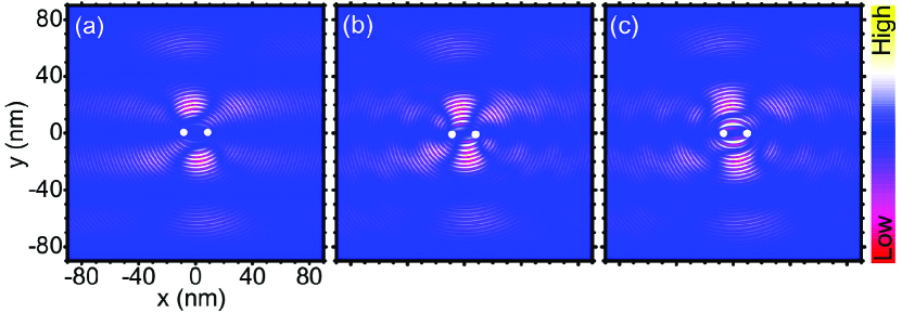
Figure 3: (Color online) Simulated STM maps of the AB oscillations of the LDOS for two identical impurities 20 nm apart on the Au(111) surface with a SOI constant $\gamma\mathtt{=}40$ meV$\cdot$nm under $B\mathtt{=}10$ T. (a) the total LDOS pattern, (b) and (c) the spin-up and spin-down components, separately. The effective electron mass $m^{\ast}\mathtt{=}0.26m_{0}$ and the Fermi wave length $\lambda_{F}\mathtt{=}3.74$ nm have been chosen.

In summary, we have performed a semiclassical analysis of the SP-STM probed AB oscillations in the LDOS induced by two impurities on a TI surface as well as on a conventional metal surface with spin splitting. We have found that the total LDOS in both systems present WL phenomenon with an oscillatory period $\Phi_{0}$ in the AB oscillations. Remarkably, the analogous WAL signified by a $\frac{\Phi_{0}}{2}$ oscillation period has been found in the spin-resolved LDOS in the TI system, while it was absent in the conventional metal surfaces. This phenomenon, which can be observed in the SP-STM experiments, may provide an important signature for the existence of the topological surface states and provide a useful criterion to distinguish the TI surface from other two-dimensional systems.

This work was supported by NSFC under Grants No. 90921003, No. 60776063, and No. 60821061, and by the National Basic Research Program of China (973 Program) under Grants No. 2009CB929103 and No. G2009CB929300.

References

- (1) C. L. Kane and E. J. Mele, Phys. Rev. Lett. 95, 226801 (2005).
- (2) B. A. Bernevig, T. L. Hughes, and S.-C. Zhang, Science 314, 1757 (2006).
- (3) M. König, S. Wiedmann, C. Brüne, A. Roth, H. Buhmann, L. W. Molenkamp, X.-L. Qi, S.-C. Zhang, Science 318, 766 (2007).
- (4) L. Fu, C. L. Kane, and E. J. Mele, Phys. Rev. Lett 98, 106803 (2007).
- (5) D. Hsieh, D. Qian, L. Wray, Y. Xia, Y. S. Hor, R. J. Cava, M. Z. Hasan, Nature 452, 970 (2008).
- (6) Y. L. Chen, J. G. Analytis, J.-H. Chu, Z. K. Liu, S.-K. Mo, X. L. Qi, H. J. Zhang, D. H. Lu, X. Dai, Z. Fang, I. R. Fisher, Z. Hussain, Z.-X. Shen, Science 325, 178 (2009).
- (7) D. Hsieh, Y. Xia, D. Qian, L. Wray, J. H. Dil, F. Meier, J. Osterwalder, L. Patthey, J. G. Checkelsky, N. P. Ong, A. V. Fedorov, H. Lin, A. Bansil, D. Grauer, Y. S. Hor, R. J. Cava, and M. Z. Hasan, Nature 460, 1101 (2009).
- (8) Y. Xia, D. Qian, D. Hsieh, L.Wray, A. Pal, H. Lin, A. Bansil, D. Grauer, Y. S. Hor, R. J. Cava, and M. Z. Hasan, Nature Phys. 5, 398 (2009).
- (9) J. E. Moore and L. Balents, Phys. Rev. B 75, 121306(R) (2007).
- (10) X.-L. Qi, T. L. Hughes, and S.-C. Zhang, Phys. Rev. B 78, 195424 (2008).
- (11) H. Zhang, C.-X. Liu, X.-L. Qi, X. Dai, Z. Fang, and S.-C. Zhang, Nature Phys. 5, 438 (2009).
- (12) E. B. Olshanetsky, Z. D. Kvon, G. M. Gusev, N. N. Mikhailov, S. A. Dvoretsky, and J. C. Potal, JETP Lett. 91, 347 (2010).
- (13) G. Tkachov and E. M. Hankiewicz, Phys. Rev. B 84, 035444 (2011).
- (14) M. Z. Hasan, H. Lin, and A. Bansil, Physics 2, 108 (2009).
- (15) H.-T. He, G. Wang, T. Zhang, I.-K. Sou, G. K. L Wong, J.-N. Wang, H.-Z. Lu, S.-Q. Shen, and F.-C. Zhang, Phys. Rev. Lett. 106, 166805 (2011).
- (16) P. Ghaemi, R. S. K. Mong, and J. E. Moore, Phys. Rev. Lett. 105, 166603 (2010).
- (17) H. Peng, K. Lai, D. Kong, S. Meister, Y. Chen, X.-L. Qi, S.-C. Zhang, Z.-X. Shen, and Y. Cui, Nature Mater. 9, 225 (2010).
- (18) J. H. Bardarson, P. W. Brouwer, and J. E. Moore, Phys. Rev. Lett 105, 156803 (2010).
- (19) Y. Zhang and A. Vishwanath, Phys. Rev. Lett. 105, 206601 (2010).
- (20) J. Chen, H.-J. Qin, F. Yang, J. Liu, T. Guan, F.-M. Qu, G.-H. Zhang, J.-R. Shi, X.-C. Xie, C.-L. Yang, K.-H. Wu, Y.-Q. Li, and L. Lu, Phys. Rev. Lett. 105, 176602 (2010).
- (21) J. G. Checkelsky, Y. S. Hor, R. J. Cava and N. P. Ong, Phys. Rev. Lett. 106, 196801 (2011).
- (22) M. Liu, C.-Z. Chang, Z. Zhang, Y. Zhang, W. Ruan, K. He, L. Wang, X. Chen, J.-F. Jia, S.-C. Zhang, Q.-K. Xue, X. Ma, and Y. Wang, Phys. Rev. B 83, 165440, (2011).
- (23) J. Wang, Ashley M. DaSilva, C.-Z. Chang, K. He, J. K. Jain, N. Samarth, X.-C. Ma, Q.-K. Xue, M. H. W. Chan, Pys. Rev. B 83, 245438 (2010).
- (24) H.-Z. Lu, J. Shi, and S.-Q. Shen, Phys. Rev. Lett. 107, 076801 (2011).
- (25) F. Meier, L. Zhou, J. Wiebe and R. Wiesendanger, Science 320, 82 (2008).
- (26) K. von Bergmann, M. Bode, A. Kubetzka, M. Heide, S. Blügel, and R. Wiesendanger, Phys. Rev. Lett. 92, 046801 (2004).
- (27) S. Schmaus, A. Bagrets, Y. Nahas, T. K. Yamada, A. Bork, M. Bowen, E. Beaurepaire, F. Evers, and W. Wulfhekel, Nat. Nanotechnology, 6, 185 (2011).
- (28) A. Cano and I. Paul, Phys. Rev. B 80, 153401 (2009).
- (29) C.-X. Liu X.-L. Qi, H. Zhang, X. Dai, Z. Fang, and S.-C. Zhang, Phys. Rev. B 82, 045122 (2010).
- (30) Q. Liu, C.-X. Liu, C. Xu, X.-L. Qi, and S.-C. Zhang, Phys. Rev. Lett. 102, 156603 (2009).
- (31) R. R. Biswas and A. V. Balatsky, Phys. Rev. B 81, 233405 (2010).
- (32) J. D. Walls and E. J. Heller, Nano Lett. 7, 3377 (2007).
- (33) B. L. Altshuler, D. Khmelnitzkii, A. I. Larkin, and P. A. Lee, Phys. Rev. B 22, 5142 (1980).