Similarity between the C¹⁸O ($J$=1–0) core mass function and the IMF in the S 140 region

Abstract

We present the results of C¹⁸O($J$=1–0) mapping observations of a $20^{\prime}\times 18^{\prime}$ area in the Lynds 1204 molecular cloud associated with the Sharpless 2-140 (S140) H ii region. The C¹⁸O cube ($\alpha$-$\delta$-$v_{\rm LSR}$) data shows that there are three clumps with sizes of $\sim$ 1 pc in the region. Two of them have peculiar red shifted velocity components at their edges, which can be interpreted as the results of the interaction between the cloud and the Cepheus Bubble. From the C¹⁸O cube data, the clumpfind identified 123 C¹⁸O cores, which have mean radius, velocity width in FWHM, and LTE mass of 0.36$\pm$0.07 pc, 0.37$\pm$0.09 km s^-1, and 41$\pm$29 M_⊙, respectively. All the cores in S140 are most likely to be gravitationally bound by considering the uncertainty in the C¹⁸O abundance. We derived a C¹⁸O core mass function (CMF), which shows a power-law-like behavior above a turnover at 30 M_⊙. The best-fit power-law index of $-2.1\pm 0.2$ is quite consistent with those of the IMF and the C¹⁸O CMF in the OMC-1 region by Ikeda & Kitamura (2009). Kramer et al. (1998) estimated the power-law index of $-$1.65 in S140 from the C¹⁸O($J$=2–1) data, which is inconsistent with this study. However, the C¹⁸O($J$=2–1) data are spatially limited to the central part of the cloud and are likely to be biased toward high-mass cores, leading to the flatter CMF. Consequently, this study and our previous one strongly support that the power-law form of the IMF has been already determined at the density of $\lesssim$ $10^{3\mbox{\scriptsize--}4}$ cm^-3, traced by the C¹⁸O($J$=1–0) line.

1 Introduction

It is believed that new stars are born in dense molecular cloud cores. Therefore, the physical properties of the dense cores are thought to be closely related to the masses of new stars to form within them. Particularly, the dense core mass function (DCMF) has been considered as a key to understanding the stellar initial mass function (IMF). Many authors have investigated the DCMFs by using dense ($\geq 10^{4\mbox{\scriptsize--}5}$ cm^-3) gas tracers such as (sub)millimeter dust continuum emission, infrared visual extinction, and molecular line emissions having high critical densities, for example, the H¹³CO⁺ ($J$=1–0) and N₂H⁺ ($J$=1–0) lines (e.g., Motte et al., 1998; Reid & Wilson, 2006; Nutter & Ward-Thompson, 2007; Rathborne et al., 2009; Ikeda et al., 2007; Walsh et al., 2007; Enoch et al., 2008). In nearby ($\leq$ 500 pc) star forming regions such as Orion, Ophiuchus, the Pipe Nebula, Perseus, and Serpens, they found that the DCMFs seem to have power-law-like behaviors in high-mass parts as $dN/dM\propto M^{-\gamma}$, whose $\gamma$ values are very similar to that of the IMF. Based on these observational facts, they propose a hypothesis that the power-law form of the IMF has been already determined at the formation stage of the dense cores.

Ikeda & Kitamura (2009) have recently discovered a similarity between the power-law forms of the IMF and the core mass function (CMF) even in the tenuous ($10^{3\mbox{\scriptsize--}4}$ cm^-3) cloud structures. They carried out mapping observations by using the C¹⁸O ($J$=1–0) line, whose critical density is 2$\times 10^{3}$ cm^-3 (Yoshida et al., 2010), toward the OMC-1 region in the Orion A cloud. They found the $\gamma$ value of the C¹⁸O CMF of 2.3 – 2.4. The $\gamma$ value is not only similar to those of the H¹³CO⁺ DCMF ($2.2\pm 0.1$; Ikeda et al., 2007) and the 850 µm dust continuum DCMF (2.2$\pm$0.2; Nutter & Ward-Thompson, 2007) within the uncertainties, but also quite consistent with that of the IMF of the Orion Nebula Cluster (2.2; Muench et al., 2002), which is associated with the OMC-1 region. The agreement between the C¹⁸O CMF and IMF $\gamma$ values suggests that, at least in the OMC-1 region, the power-law form of the IMF with $\gamma\geq 2$ has been maintained from the formation time of the tenuous structure with density of $\sim 10^{3\mbox{\scriptsize--}4}$ cm^-3. In addition to the Orion cloud, a representative of massive star formation, the similarity between the CMF and the IMF was reported in low-mass star forming regions by Tachihara et al. (2002). The C¹⁸O cores found in Taurus, Chamaeleon, Lupus, and other low-mass star forming regions show the CMF with $\gamma$ = 2.6 above 56 M_⊙.

Kramer et al. (1998), however, found a significantly smaller $\gamma$ value of 1.7 for the S140 and M17SW regions by using the C¹⁸O ($J$=2–1) line with a high critical density comparable to that of H¹³CO⁺ ($J$=1–0). Wong et al. (2008) also found $\gamma$ = 1.7 in the C¹⁸O ($J$=1–0) CMF of RCW 106. In this study, we focus on S140 for the following reasons. First, the distance to S140 of 910 pc (Crampton & Fisher, 1974) is the nearest one of them; the distances to M17SW and RCW 106 are 2.2 kpc (Chini et al., 1980) and 3.6 kpc (Lockman, 1979), respectively, and the two clouds are located in the Sagittarius arm. Since we discuss the power-law nature of the CMF on the basis of a comparison with that in OMC-1, it seems quite natural to first select the S140 region, located in the Local (Orion) Spur as the next step in our CMF study. Second, since the previous C¹⁸O ($J$=2–1) observations of S140 (Johnen, 1992) covered only the brightest $4^{\prime}\times 4^{\prime}$ region around IRAS 22176+6303, we cannot exclude the possibility that their core identification was biased to high-mass cores, leading to the flatter CMF. Third, the higher transition of $J$=2–1 with the transition energy of 15.8 K might prefer to pick up higher-mass protostellar cores, compared to the lowest transition of $J$=1–0.

The aim of this paper is to re-estimate the power-law index of the CMF in the S140 region, also identified as Lynds 1204, and to examine whether the similarity between the CMF and the IMF holds in the region or not. Our observations were done to cover the cloud as widely as possible, in order to avoid the possible spatial bias. We employed the C¹⁸O ($J$=1–0) line emission, which is the same tracer as Ikeda & Kitamura (2009) did, and is suitable for deriving the tenuous CMF (e.g., Tachihara et al., 2002). Furthermore, we used the clumpfind algorithm (Williams et al., 1994), the same core identification method as that Ikeda & Kitamura (2009) employed, to directly compare with their results. Note that the spatial resolution is high enough to evaluate the CMF at the distance to the S140 region of 910 pc, as shown in §5.

In §2, we describe the details of our observations. In §3, we show the overall spatial and velocity structures of the tenuous gas traced by the C¹⁸O ($J$=1–0) emission in the S140 cloud, and identify three clumps with sizes of $\sim$ 1 pc. In §4 we describe the identification of the C¹⁸O cores in S140, and discuss their physical properties by comparing with those in the OMC-1 region. We show the C¹⁸O ($J$=1–0) CMF in §5. In this section, we compare our CMF with the previous $J$=2–1 CMF, and discuss the similarity between the C¹⁸O (1–0) CMF and the IMF. In §6 we summarize our results.

2 Observations

The C¹⁸O ($J$=1–0) mapping observations were carried out in the period from January to February 2010 by using the Nobeyama 45 m radio telescope. Our map covered a $20^{\prime}\times 18^{\prime}$ area, whose center was selected to be 22^h20^m18^s, 63^∘22^′12^′′ (J2000). Using the On-The-Fly technique (Sawada et al., 2008), we swept the area by raster scan with a scan speed of the telescope of 35 arcsec s^-1. To reduce scanning effects, we scanned in both the RA and Dec directions. At the frequency of the C¹⁸O ($J$=1–0) emission (109.782182 GHz; Ungerechts et al., 1997), the half power beam width, $\Delta\theta_{\rm HPBW}$, and main beam efficiency, $\eta$, of the telescope were 14^′′ and 0.4, respectively. By the standard chopper-wheel method, the receiver intensity was converted into the antenna temperature $T_{\rm{A}}^{*}$, corrected for the atmospheric attenuation. We used an off position of 22^h18^m34^s, 63^∘2^′12^′′, where we could not the C¹⁸O emission above 0.09 K in $T_{\rm{A}}^{*}$. At the front end, we used the 25-BEam Array Receiver System (BEARS) in double-sideband (DSB) mode, which has 5$\times$5 beams separated by 41^′′.1 in the plane of the sky (Sunada et al., 2000; Yamaguchi et al., 2000) . The 25 beams have beam-to-beam variations of about 10% in both beam efficiency and sideband ratio. To correct for the beam-to-beam gain variations, we calibrated the intensity scale of each beam by observing the W3 region with a 100 GHz SIS receiver (S100) with a single-sideband filter. At the back end, we used 25 sets of 1024 channel autocorrelators (ACs), which have a velocity resolution of 0.104 km s^-1 at 110 GHz (Sorai et al., 2000). Since the data dumping time of the ACs was 0.1 s, the spatial data sampling interval on the sky plane was 3.5^′′. The spatial interval corresponds to 0.3$\Delta\theta_{\rm HPBW}$, and is small enough to satisfy the Nyquist theorem. The telescope pointing was checked every 1.5 hours by observing the SiO ($v$=1, $J$=1–0; 43.122 GHz) maser source T–Cep. Since the pointing uncertainty of the telescope remains as small as a few arcseconds below a wind speed of 5 m s^-1, we rejected the data taken under the condition that the wind speed averaged over one minute exceeds 6 m s^-1. Consequently, the pointing accuracy is better than 3^′′ for the data to be analyzed.

To construct an $\alpha$-$\delta$-$v_{\rm LSR}$ data cube with spatial and velocity resolutions of 22^′′ and 0.1 km s^-1 in full width half maximum (FWHM), we used a Gaussian function as a gridding convolution function (GCF) to integrate the spectra which were taken with the very high spatial sampling rate of 3.5^′′. We adopted 17^′′.0 as the size of the GCF in FWHM. The resultant effective spatial resolution of the cube, $\Delta\theta_{\rm eff}$ becomes 22^′′.0, corresponding to 0.1 pc at the distance to the S140 region. Since the DSB system noise temperature ranged from 285 to 357 K with a mean value of 321 K during the observations, we have an rms noise level of the data cube of 0.12 K in $T_{\rm{A}}^{*}$.

3 C¹⁸O ($J$=1–0) map of the S140 region

In this section we describe the overall spatial and velocity structures of the C¹⁸O ($J$=1–0) emission in the S 140 region. In addition, we identify three distinct clumps with sizes of $\sim$ 1 pc, which is likely to be the natal objects for clusters.

3.1 Spatial and Velocity Structures of the C¹⁸O ($J$=1–0) emission

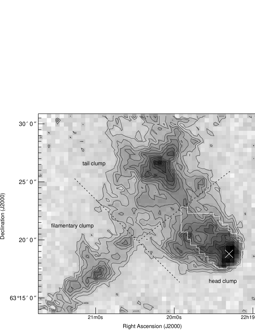
Figure 1: Total integrated intensity map of the C¹⁸O ($J$=1–0) emission ( $\upsilon_{\rm{LSR}}$= $-9.9$ - $-4.8$ km s^-1) in the S 140 region. The contour intervals are 0.25 K km s^-1 (corresponding to 2$\sigma$) starting at 0.5 K km s^-1. The gray scale bar is shown at the right-hand side of the panel. The white cross indicates the position of IRAS 22176+6303. The white polygon shows the mapping region in C¹⁸O ($J$=2–1) by Johnen (1992). The dashed lines roughly indicate the boundaries of the head, tail, and filamentary clumps (see §3.1).

Figure 1 shows the total integrated intensity map of the C¹⁸O ($J$=1–0) emission of the S140 region. The total mass of the cloud is estimated to be 6600 M_⊙ (see §4.1 for details). One can see three distinct peaks, referred to as head, tail and filamentary clumps in this paper. The main body of the cloud is known as a cometary one, and our map clearly shows the cometary shape; the C¹⁸O emission is the brightest toward the head clump, which faces the Sh-2 140 H ii region and is associated with IRAS 22176+6303, indicated by the cross mark in Figure 1. The head clump is also known as an active cluster-forming region where numerous young stellar objects have been identified in infrared wavelength (Megeath et al., 2004). On the other hand, the tail clump seems streaming toward the north-east. In contrast to the head clump, no active star formation is known within the tail clump, although no sensitive infrared observations have been published yet. Since our map covers a wider region by a factor of three than those of the previous molecular line mapping observations (Ridge et al., 2003; Higuchi et al., 2009), we found another filamentary clump located on the south-east of the cometary cloud. Note that the elongation of the filamentary clump seems perpendicular to the head-tail direction of the cometary cloud. Although the filamentary clump can be seen in a previous large-scale survey with the spatial resolution of several arcminutes (Yonekura et al., 1997), our map is the finest one resolving 0.1 pc-scale cores.

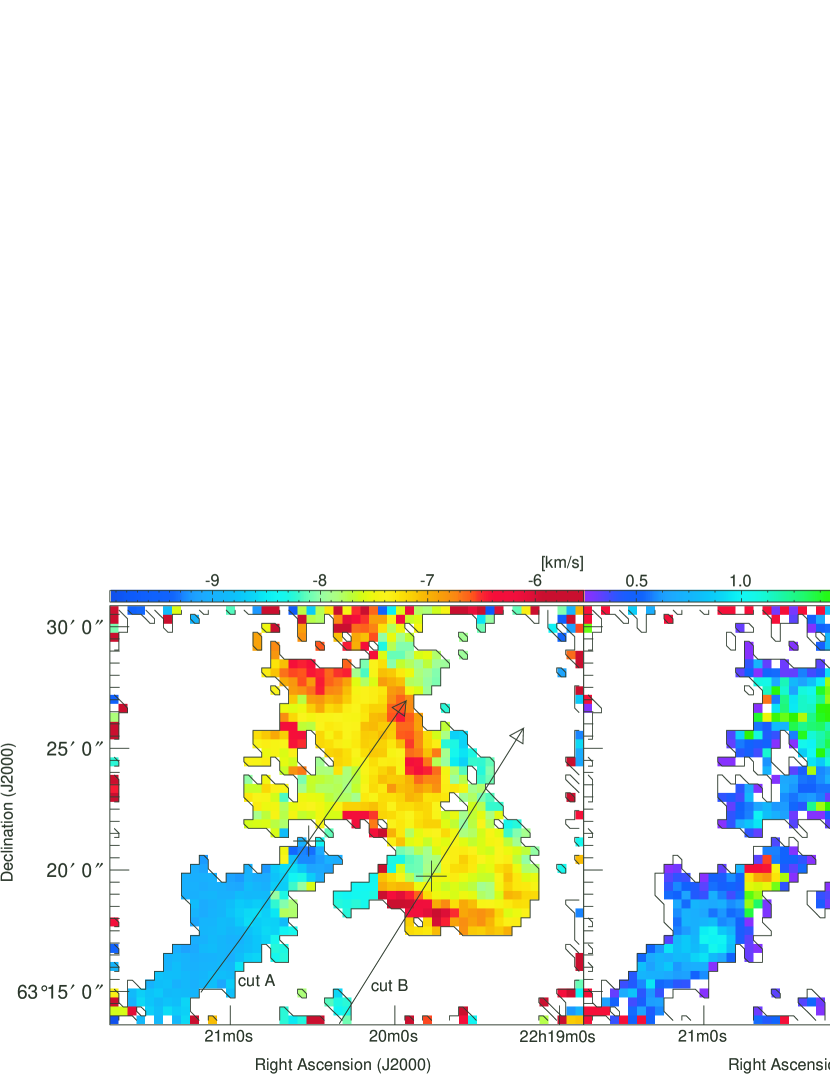
Figure 2: (Left) Map of the intensity-weighted mean LSR velocity, i.e., the centroid velocity map for the C¹⁸O ($J$=1–0) emission in the S 140 region. (Right) Map of the velocity width in FWHM. The color bar is shown at the top of each panel. In the left panel, the arrows indicate the cutting lines of the position-velocity diagrams in Figure 3. The cross marks on the arrows show the origins of the position axis for the position-velocity diagrams. The centroid velocity and the velocity width are calculated within the areas above the 3 $\sigma$ noise level: the thin solid polygons delineate the 3 $\sigma$ noise level in Figure 1 (see also Yoshida et al. (2010)).

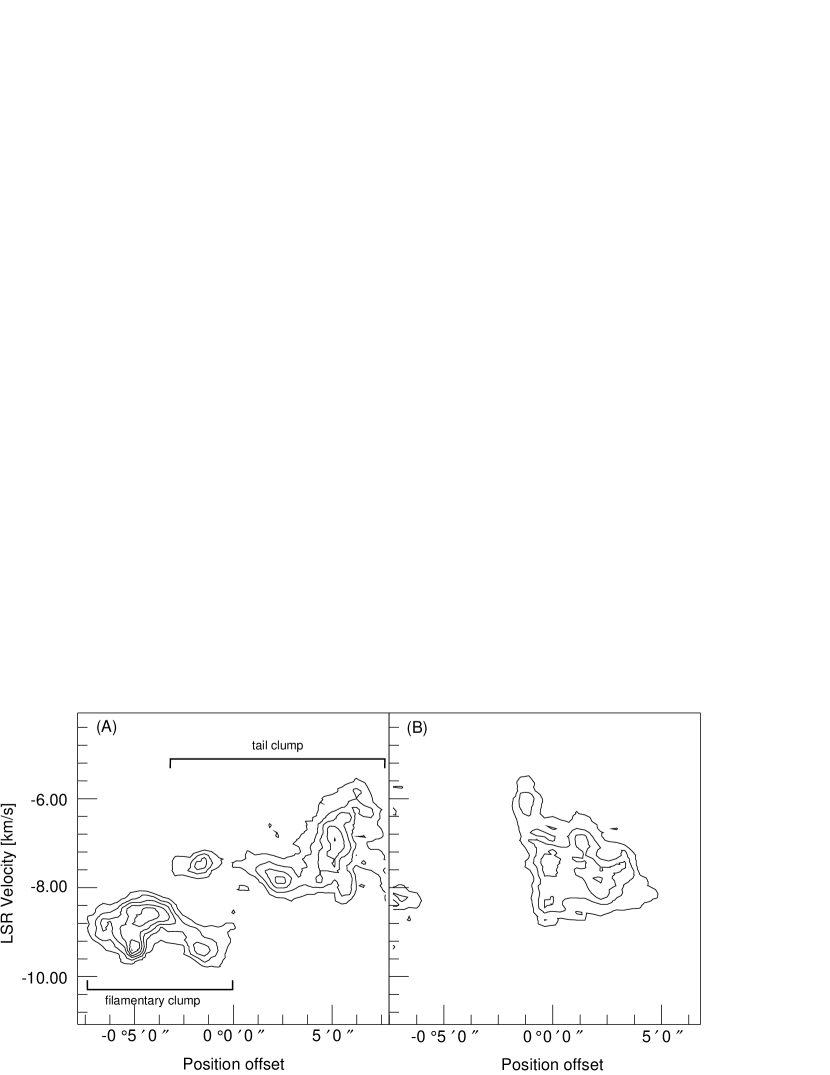
Figure 3: Position-velocity diagrams of the C¹⁸O ($J$=1–0) emission along the cutting lines A (left) and B (right) indicated in Figure 2. The origins of the position axes are indicated by the cross marks in Figure 2. The contour intervals are 0.25 K (corresponding to 2$\sigma$) starting at 0.38 K (3 $\sigma$).

As shown in Figure 2, we calculate the intensity-weighted mean LSR velocity, i.e., the centroid velocity, and velocity width in FHWM of the C¹⁸O emission at each spatial grid point in Figure 1, following Yoshida et al. (2010). The centroid velocity map illustrates that the centroid velocities in the cometary cloud range from $-8.5$ to $-6.0$ km s^-1, while the filamentary clump has a more blue-shifted velocity range from $-10.0$ to $-8.0$ km s^-1. The mean velocity width all over the cometary cloud is 1.0 km s^-1, and the largest velocity width of 2.5 km s^-1 is found toward the IRAS source, which is probably related to the star formation activity in the head clump. On the other hand, the velocity width of the filamentary clump is as small as 0.6 km s^-1. However, the velocity width map apparently shows a somewhat large velocity width of $\sim$ 2.5 km s^-1 at $\alpha,\delta$ = 22^h20^m43^s, 63^∘20^′0^′′ in the filamentary clump. As indicated in the position-velocity diagram of Figure 3A, this is because a component belonging to the cometary cloud with a mean LSR velocity of $\sim$ $-7.5$ km s^-1 overlaps with the filamentary clump with a mean LSR velocity of $\sim$ $-9.0$ km s^-1 along the line of sight. Note that the velocity width of each components is as small as $\sim$ 0.5 km s^-1 at this point.

The centroid velocity map indicates that there are red-shifted components of $\upsilon_{\rm{LSR}}$ = $-7\>\sim\>-6$ km s^-1 on the periphery of the cometary cloud. Among the red-shifted components, the most prominent one can be found in the southern edge of the head clump. The red-shifted component of $-6$ km s^-1, for example, is more easily recognized in the position-velocity diagram of Figure 3B. Since the S140 region faces the Cepheus Bubble and the cloud exhibits the cometary shape, the region is likely to interact with the expanding bubble driven by stellar winds and supernova explosions of members of Cep OB2 (Ábrahám et al., 2000). Therefore, the red-shifted components around the cometary cloud can be interpreted as the outer envelope of the cloud that has been pushed toward the far side along the line of sight by the expanding bubble. However, the velocity widths of the red-shifted components of $\sim 0.5$ km s^-1 never exceed that of the main body of the cometary cloud. Since the expanding velocity of the bubble of 10 km s^-1 (Ábrahám et al., 2000) is an order of magnitude larger than the thermal motion of the cloud, it is expected that the interaction is associated with shocks, leading to large velocity width. The small velocity widths of the red-shifted components might imply that the turbulent motions excited by the interaction in the red-shifted components have been already dissipated with a crossing time as short as 7$\times 10^{4}$ yr (see also a discussion in §4.2).

3.2 Identification of Clumps for Cluster Formation

Lada & Lada (2003) showed that the clumps with sizes of $\sim$ 1 pc and masses of the orders of $10^{2}$ – $10^{3}$ M_⊙ are the natal objects for the stellar clusters. The three clumps in S140, the head, tail and filamentary clumps can be considered as the cluster-forming clumps, though active cluster formation has been found only in the head clump. This is because their sizes are about 1 pc and the masses are of the order of $10^{3}$ M_⊙. Actually, the masses of the head, tail, and filamentary clumps are estimated to be 2200, 2600, and 1800 M_⊙, respectively, from the total integrated intensities with $\upsilon_{\rm{LSR}}$ = $-$9.9 – $-4.8$ km s^-1 of the areas above the 2 $\sigma$ noise level in Figure 1 (the details of the mass estimation is shown in §4.1). Previously, Ridge et al. (2003) and Higuchi et al. (2009) mapped the head clump by using the C¹⁸O ($J$=1–0) line, and the clump mass was estimated to be 1900 M_⊙ by Higuchi et al. (2009), which is roughly consistent with ours.

Our interpretation that the three clumps in S140 are the site of cluster formation is also supported by the following virial analysis. Assuming the clumps are spherical, we derived the virial masses of 1100, 1300, 330 M_⊙ with the uncertainty of a factor of 3 for the head, tail, and filamentary clumps, respectively. Since the clump masses are twice or more larger than the virial masses, it is most likely that the clumps are gravitationally bound and have the potential for producing clusters. In addition, the whole cloud of S140 is also in gravitationally bound state. By using the mean velocity width of 1.95 km s^-1 in FWHM all over the cloud and the projected extent of the cloud of 3.7 pc of the cloud, the virial mass of the cloud is estimated to be 1900 M_⊙, which is by a factor of three smaller than the cloud mass of 6600 M_⊙.

4 C¹⁸O core catalog

4.1 Identification of the Cores and Derivation of Their Physical Properties

Following the C¹⁸O CMF study in the OMC-1 region (Ikeda & Kitamura, 2009), we applied the clumpfind algorithm (Williams et al., 1994) to the C¹⁸O three-dimensional ($\alpha$-$\delta$-$v_{\rm LSR}$) cube data. The algorithm can work well with reasonable parameters to identify cores or clumps, though several authors pointed out some shortcomings of the clumpfind. Pineda et al. (2009) examined the behavior of the algorithm by changing the threshold level from 3 to 20 $\sigma$, a wider range than Williams et al. (1994) examined, and found that the power-law index of the mass function sensitively depends on the threshold for higher thresholds of $>$ 5 $\sigma$. However, Ikeda & Kitamura (2009) demonstrated the weak dependence of core properties and CMF on the threshold in the reasonable range from 2 to 5 $\sigma$ levels, which had been also shown in Pineda et al. (2009). Therefore, we adopted the threshold level for the algorithm of 0.24 K, i.e., the 2 $\sigma$ noise level of the cube data, which is recommended for identifying the core structure by Williams et al. (1994) and falls in the robust and reasonable range derived by Ikeda & Kitamura (2009). We adopted the grid spacing of the cube data of 22^′′.0, equal to $\Delta\theta_{\rm eff}$, i.e., full-beam sampling. This is because Williams et al. (1994) determined the optimal threshold of the 2 $\sigma$ level for the full-beam sampling case. We also used the additional criteria introduced in Ikeda et al. (2007) to reject ambiguous or fake core candidates whose size and velocity width are smaller than the spatial and velocity resolutions, respectively.

We identified 123 cores and estimated the beam-deconvolved radius $R_{\rm core}$, velocity width in FWHM corrected for the spectrometer resolution $dv_{\rm core}$, LTE mass $M_{\rm core}$, virial mass $M_{\rm vir}$, and mean density $\bar{n}$ of the C¹⁸O cores. Table 1 shows the physical properties of the C¹⁸O cores in S140. The definitions of these parameters are the same as those in Ikeda & Kitamura (2009). Here we briefly summarize the parameters specific to this study. We adopted $\Delta\theta_{\rm eff}$ $=22^{\prime\prime}.0$ as described in §2, the antenna efficiency $\eta$ of 0.4, and the fractional abundance of C¹⁸O relative to H₂, $X_{\rm C^{18}O}$ of $1.7\times 10^{-7}$ (Frerking et al., 1982). The optical depth of the C¹⁸O line in the S140 region has been estimated to be smaller than 1; Higuchi et al. (2009) derived the upper limit of the optical depth of 0.5, from the intensity ratio of the C¹⁸O ($J$=1–0) to C¹⁷O ($J$=1–0) lines. We assumed that the excitation temperature $T_{\rm ex}$ is uniform over the S140 region and is equal to the rotational temperature of 24 K in the NH₃ (1, 1) and (2, 2) observations by Higuchi et al. (2009). In the head clump, the temperature of $>$ 20 K is reasonable because the clump faces the Sh 2-140 H ii region and numerous young stellar objects have been found (Megeath et al., 2004), as well as the OMC-1 cloud. On the other hand, the other two clumps have not been well studied compared to the head clump. In the filamentary clump, two IRAS point sources 22192+6302 and 22196+6302 are detected, but the nature of the sources is unknown. Toward the tail clump, no signature of star formation has been found. Although our assumption of the uniform temperature cannot be validated for the two clumps, we found that a low $T_{\rm ex}$ value of 10 K does not seriously affect our discussion, and therefore we adopted the assumption of the uniform $T_{\rm ex}$ in this study.

4.2 Physical Properties of the C¹⁸O Cores

We discuss the physical properties of the C¹⁸O cores on the basis of comparison with those of the C¹⁸O cores in the OMC-1 region of the Orion A cloud (Ikeda & Kitamura, 2009). To fairly compare the S140 C¹⁸O cores with the OMC-1 C¹⁸O ones, we smoothed the OMC-1 data by a Gaussian function with a FWHM size of 37^′′.3 so that the OMC-1 cloud is put at the distance of 910 pc to S140. Furthermore, we randomly picked up 25 % of the original spectra to make the cube data for OMC-1 so as to have the same signal to noise ratio as that of the S140 data. Finally we re-identified 44 C¹⁸O cores from the smoothed cube data in OMC-1.

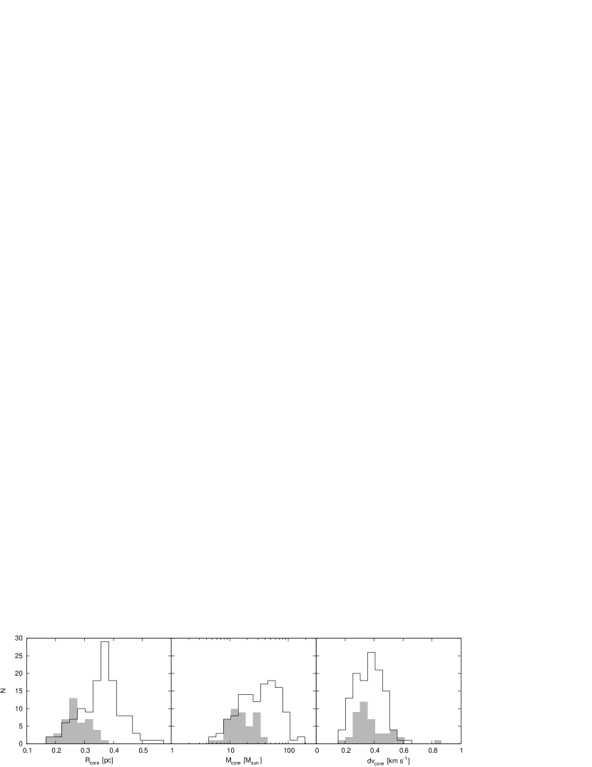
Figure 4: Histograms of $R_{\rm core}$ (left), $M_{\rm core}$ (middle), and $dv_{\rm core}$ (right) of the C¹⁸O cores. The open and gray histograms mean the C¹⁸O cores in the S 140 region and those in the smoothed OMC-1 data (see §4.2), respectively.

The left panel of Figure 4 shows that the $R_{\rm core}$ distribution of the C¹⁸O cores in S140 has a single peak at 0.37 pc, which is much larger than the peak radius of 0.26 pc in OMC-1: the mean value of 0.36$\pm$0.07 pc for $R_{\rm core}$ in S140 is larger than that in OMC-1 of 0.27$\pm$0.05 pc. The Kolmogorov-Smirnov (K-S) test applied to the $R_{\rm core}$ histograms demonstrates that the distributions are considerably different from each other with a significance level of 1 %. The mass $M_{\rm core}$ of the C¹⁸O cores in the S140 region tends to be also larger than that in OMC-1, as shown in the middle panel of Figure 4; the mean value in S140 of 41$\pm$29 M_⊙ is twice larger than that in OMC-1 of 18$\pm$9 M_⊙. In addition, the K-S test shows that the two distributions are considerably different from each other. Although only one broad peak at $\sim$ 20 M_⊙ seems to exist for OMC-1, we can see two broad peaks at $\sim$ 20 M_⊙ and $\sim$ 50 M_⊙ for S140.

The above comparisons suggest that the large ($R_{\rm core}$ $>$ 0.4 pc) and massive ($M_{\rm core}$ $>$ 50 M_⊙) cores exist only in the S140 region. Furthermore, the mass fraction of the cores in S140 is very large: the total mass of the C¹⁸O cores is 5000 $M_{\odot}$, 75% of the total mass traced by the C¹⁸O emission (see §3.2). This fraction is twice larger than that of the C¹⁸O cores in OMC-1 (Ikeda & Kitamura, 2009), but is roughly consistent with the fraction of 60 % for the H¹³CO⁺ cores (Ikeda et al., 2007, 2009). The large massive cores and the high mass fraction of the cores in the S140 region are likely to be caused by high column densities in the region. Actually, the C¹⁸O ($J$=1–0) peak intensity of 2.4 K in $T_{\rm{A}}^{*}$ in S140 is significantly larger than that in the OMC-1 region of 1.6 K. It is possible to interpret that the accumulation of interstellar matter occurred owing to the interaction between the S140 cloud and the expanding Cepheus Bubble, as suggested by the cometary shape and velocity features of the cloud as described in §3.1.

The $\bar{n}$ range of 1.0 to 9.8$\times 10^{3}$ cm^-3 for the C¹⁸O cores in S140 is similar to that in OMC-1 of 2.3 to 9.3$\times 10^{3}$ cm^-3, and is consistent with the critical density of the C¹⁸O ($J$=1–0) line of $\sim$ 2$\times 10^{3}$ cm^-3 (Yoshida et al., 2010). In addition, Rathborne et al. (2009) showed that the mean volume density of their C¹⁸O cores in the Pipe nebula is 7.3$\times 10^{3}$ cm^-3, which falls in our $\bar{n}$ ranges of (1.0–9.8)$\times 10^{3}$ cm^-3. In spite of the large range of $\bar{n}$, the traced the traced densities of $\lesssim$ 10⁴ cm^-3 is significantly smaller than those of the dense gas tracers used by the previous CMF studies mentioned in §1.

In contrast to $R_{\rm core}$ and $M_{\rm core}$, the distribution of the velocity width $dv_{\rm core}$ in S 140 is quite similar to that in OMC-1, as shown in the right panel of Figure 4. The K-S test shows that there is no considerable difference with a significance level of 1 %. The mean value of $dv_{\rm core}$ in S 140 is 0.37$\pm$0.09 km s^-1 and is almost the same as that in OMC-1 of 0.38$\pm$0.12 km s^-1. It is likely that the turbulent motions excited by the passing of the expanding bubble have been already damped, though the bubble could significantly increase the velocity width of the C¹⁸O cores. Considering the total kinetic energy of the bubble is 2.7$\times 10^{50}$ erg in H i gas, the distance to the bubble center is 910 pc, and the radius of the bubble is 5 degree (Ábrahám et al., 2000), the kinetic energy injected into the C¹⁸O cores with a mean radius of 0.36 pc can be estimated to be 1.7$\times 10^{46}$ erg, leading to a large velocity width of 1.2 km s^-1; such the large value of $dv_{\rm core}$ cannot be discerned in the right panel of Figure 4. Here, we assume that the fraction of the injected kinetic energy to be converted into turbulence is 0.01 to 0.05 (Mac Low & Klessen, 2004; Ikeda et al., 2007). Since the expansion velocity of the bubble is 10.2 km s^-1 (Ábrahám et al., 2000), the crossing time of the bubble over the cores is estimated to be as short as 7$\times 10^{4}$ yr, much smaller than the age of 1.7 Myr for the bubble (Ábrahám et al., 2000). Therefore, one can expect the dissipation of the turbulent motions within the cores at the present time.

In the left panel of Figure 5 we show the $dv_{\rm core}$-$R_{\rm core}$ relation of the C¹⁸O cores. Although the distribution of the S140 cores tends to shift toward larger radii, as shown in Figure 4, both the distributions in S140 and OMC-1 seem to be similar to each other. Actually, the best-fit power-law function for S140 is ($dv_{\rm core}$/km s^-1) = (0.65$\pm$0.07)$\times$($R_{\rm core}$/pc)^0.58±0.11 with a small correlation coefficient of 0.39, and the best-fit one for the OMC-1 cores is ($dv_{\rm core}$/km s^-1) = (0.55$\pm$0.21)$\times$($R_{\rm core}$/pc)^0.32±0.25 with a correlation coefficient of 0.22; the two best-fit functions are consistent with each other within the uncertainties. In the right panel of Figure 5 we show the correlation between the virial ratio, $M_{\rm vir}$$/$$M_{\rm core}$, and $M_{\rm core}$. Since the mean value of the virial ratio is 0.3$\pm$0.2 in S140, all the C¹⁸O cores are likely to be gravitationally bound by considering the uncertainty in $X_{\rm C^{18}O}$ of a factor 3. Both the data in S140 and OMC-1 show negative correlations; the best-fit power-law function of the S140 cores is ($M_{\rm vir}$/$M_{\rm core}$) = (1.27$\pm$0.25)$\times$($M_{\rm core}$/M_⊙)^-0.43±0.06, with a correlation coefficient of 0.48. A similar negative correlation in the C¹⁸O ($J$=1–0) data is also found in low-mass star forming regions of Taurus, Ophiuchus, Lupus, L1333, Chamaeleon and the Pipe Nebula (Tachihara et al., 2002). The power-law index of $-$0.43 is shallower than the value of $-2/3$ expected for “pressure-confined” structures derived by Bertoldi & McKee (1992). This fact also suggests that the self-gravity is dominant in the S140 C¹⁸O cores, compared to the ambient pressure, unlike the $\rho$ Ophiuchi case by Maruta et al. (2010).

5 C¹⁸O CMF in the S140 region

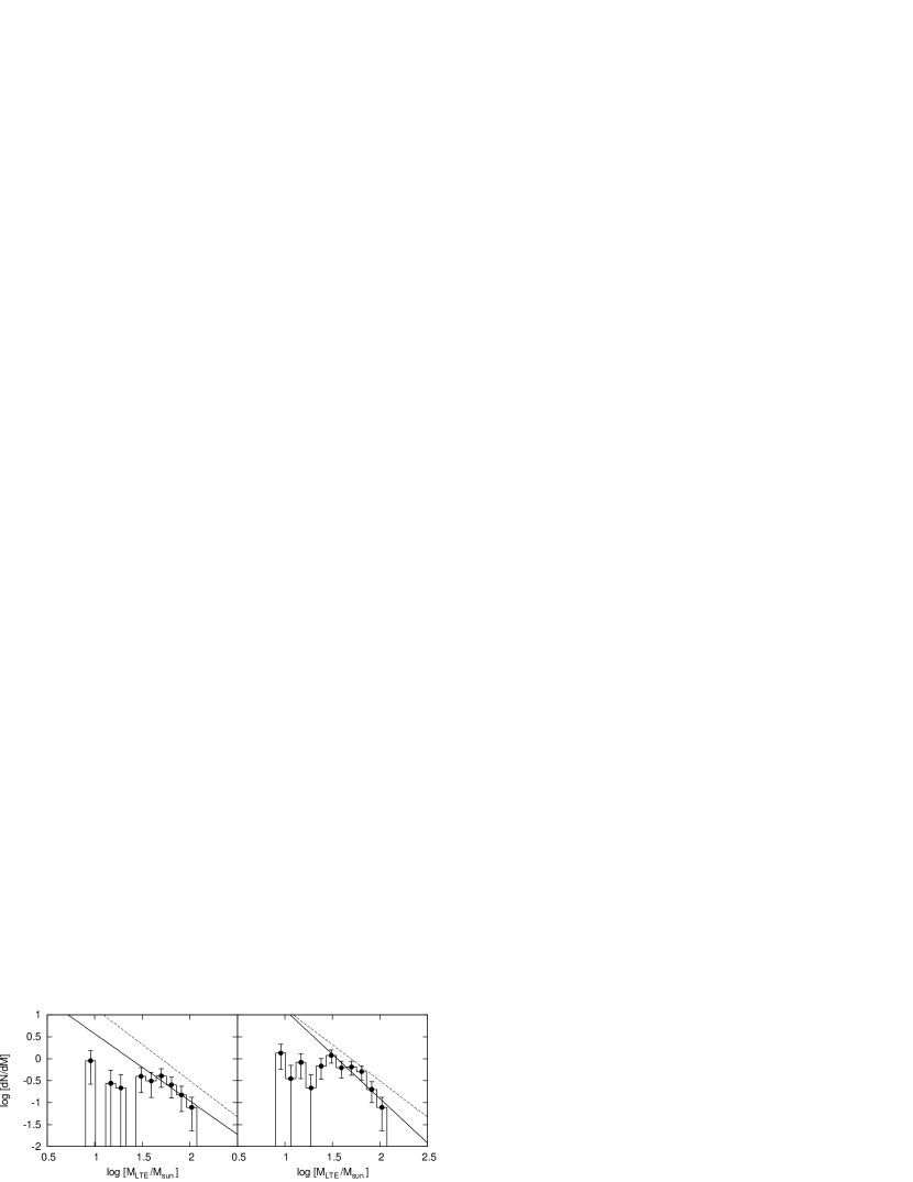
Figure 7: (Left) Mass function of the C¹⁸O cores identified in the mapping region by Johnen (1992) in the C¹⁸O ($J$=2–1) line. Note that the mass bins are the same as those in Figure 6. The solid line indicates the best-fit power-law function above 30 M_⊙, and the dashed line a power-law function with the index of $-1.65$, which was derived from the C¹⁸O ($J$=2–1) data by Kramer et al. (1998). (Right) Mass function of the C¹⁸O cores identified all over the head clump. The solid line shows the best-fit power-law function above 30 M_⊙, and the dashed one is the same as in the left panel.

Figure 6 shows a CMF of the C¹⁸O cores. The CMF has a turnover at around 30 M_⊙, and a power-law-like shape in the high-mass part above the turnover. Above 30 $M_{\odot}$, we applied a single power-law function by considering the statistical uncertainties and found that the best-fit power-law index $\gamma$ is 2.1$\pm$0.2. However, the $\gamma$ value significantly differs from that of the C¹⁸O ($J$=2–1) CMF in the S140 region of $\gamma$ = 1.65$\pm$0.18 (Kramer et al., 1998). We consider that this difference is likely due to their limited observation area in core survey. As shown in Figure 1, it is apparent that the area of the C¹⁸O ($J$=2–1) observations (Johnen, 1992) covers only the central intense part of the head clump, where the C¹⁸O intensities are relatively stronger than those in the other areas in the S140 region, and the core identification is likely to be biased to massive cores. To examine this possibility, we re-identifed 26 C¹⁸O ($J$=1–0) cores within the C¹⁸O ($J$=2–1) mapping area, and we re-estimated the CMF from the 26 cores, as shown in the left panel of Figure 7. Although our spatial resolution of 22^′′ is twice coarser than that of the C¹⁸O ($J$=2–1) study of 13^′′ (Johnen, 1992; Kramer et al., 1998) and hence our statistical uncertainties are large in the low-mass part of $\leq$ 30 M_⊙, the CMF shows a power-law-like behavior in the high-mass part. The best-fit $\gamma$ is 1.5$\pm$0.6 and is consistent with the previous value of 1.65 derived by Kramer et al. (1998). Furthermore, we estimated the CMF all over the head clump. There are 44 cores in the head clump and the best-fit $\gamma$ is 2.0$\pm$0.4, as shown in the right panel of Figure 7. Although the core numbers are not sufficiently large for the statistical analysis, the $\gamma$ value in the head clump tends to be larger than that in the central intense part of the head clump, and are consistent with that of all the C¹⁸O cores in our observed region. Therefore, we conclude that the CMF should be estimated from the mapping data that covers at least one clump, which is thought to be the natal structure of a stellar cluster (Lada & Lada, 2003).

Our $\gamma$ value of 2.1$\pm$0.2 is consistent with that of the C¹⁸O CMF in the OMC-1 region (Ikeda & Kitamura, 2009). This agreement confirms that our observations could resolve star-forming cores even at the large distance of $\sim$ 1 kpc. A poor spatial resolution is one of the major causes of the underestimation of $\gamma$. To examine the dependence of $\gamma$ on the spatial resolution, we created the smoothed OMC-1 C¹⁸O data cubes by changing the effective resolutions, as described in §4.2, and derived the $\gamma$ values for the smoothed cubes, as shown in Figure 8. It is clearly shown that our resolution of 22^′′, corresponding to 0.097 pc for S140, can correctly estimate the $\gamma$ value within the uncertainties. Actually, our $\gamma$ value is consistent with that in the C¹⁸O study by Tachihara et al. (2002), having a spatial resolution enough to resolve 0.1 pc-scale cores. In addition, Figure 8 predicts that $\gamma$ is considerably underestimated for the case that $\Delta\theta_{\rm eff}$ becomes larger than 0.1 pc, which is the minimum radius of the cores in the OMC-1 region at the highest resolution of 0.061 pc. Therefore, the small $\gamma$ value of $\sim$ 1.7 in RCW 106 (Wong et al., 2008) is likely due to the coarse spatial resolution of 0.78 pc at the distance of 3.6 kpc (Lockman, 1979).

This study concludes that the power-law shape with $\gamma$ $>$ 2 in CMF holds even in tenuous structures with the densities of 10${}^{3\mbox{\scriptsize--}4}$ cm^-3 of the S140 region, in addition to our recent work by Ikeda & Kitamura (2009) in OMC-1. Furthermore, the $\gamma$ values of the C¹⁸O CMFs in S140 and OMC-1 are quite consistent with that of the Galactic field-averaged IMF of 2.3$\pm$0.7 (Kroupa, 2001). These observational facts lead us to the hypothesis that the power-law nature in the IMF originates in molecular cloud structures with densities of less than $\sim 10^{3\mbox{\scriptsize--}4}$ cm^-3.

Our conclusion of the resemblance between the CMF and the IMF is consistent with the recent theoretical works showing that such a resemblance should be understood as a statistical relation, rather than a one-to-one correspondence between a core and a star to be formed within it. Smith et al. (2009) examined the formation and evolution of gravitationally-bounded cores by SPH simulations and found that the initial masses of the cores have a poor correlation with the resultant stellar masses. However, the shape of the CMF is maintained throughout the simulations and the resultant IMF shape is quite consistent with the initial shape of the CMF (see also Chabrier & Hennebelle, 2010). Furthermore, Swift & Williams (2008) presented a supporting result that the resultant IMFs are insensitive to the differences in theoretical models for star formation within cores and that the input shape of the CMF is kept until the IMF within the current observational uncertainties.

Since our studies are limited to the two clouds of S140 and OMC-1 up to now, it is urgent to perform systematic studies of the tenuous CMFs in various star forming regions. Since the S140 and OMC-1 regions are massive star/cluster forming ones, it is interesting to explore the CMF shape in regions where no star formation activity is found because stellar feedback processes, such as outflow, stellar wind, and expanding H ii region may cause some influence on the physical properties of the tenuous structures (e.g., Nakamura & Li, 2007). Although the global S140 cloud and the individual C¹⁸O cores are likely to be influenced by the Cepheus Bubble as shown in §3.1 and 4.2, we cannot examine whether the CMF shape is affected by the bubble or not only from our S140 data. Recently, Rathborne et al. (2009) estimated the DCMF in the Pipe Nebula, where no active star formation occurs, and found that the DCMF shape including the slope in the high-mass part is quite consistent with that of the IMF derived in the Orion Nebula Cluster associated with the OMC-1 cloud (Muench et al., 2002), where the most active star formations occur in the solar neighborhood. This study suggests that the stellar feedback processes seem not to play a dominant role in determining the CMF shape.

For future observations of the tenuous CMFs, we require the following two points on the basis of our results. First, mapping observations should not be spatially biased. We have shown that the lower value of $\gamma$ in the C¹⁸O ($J$=2–1) CMF previously estimated in the S140 region is likely to be caused by the limited mapping area only for the intense portion of the cloud. Second, observations should be done with a high spatial resolution enough to resolve the 0.1 pc-scale core structures, as shown in Figure 8. To further investigate the CMFs over the Galactic disk, one should extend the studies in the solar neighborhood to those in regions where environmental conditions, such as metallicity, interstellar radiation, and turbulence, are different (Krumholtz et al., 2010; Schmidt et al., 2010). The first step would be toward the neighbor, Sagittarius/Perseus arms. Actually, in M17SW and RCW 106 which are located in the Sagittarius arm, smaller power-law indices of the CMFs of $\sim 1.7$ have been reported (Kramer et al., 1998; Wong et al., 2008). To do observations of cores in the Sagittarius arms, approximately 2.0 kpc apart from the sun, we need an angular resolution of 10^′′ to achieve a linear spatial resolution of 0.1 pc. Furthermore, an extreme environment is known in the Galactic center region. The Arches cluster, associated with the Galactic center, shows the present-day mass function with $\gamma$ of $<2$, which is significantly flatter than that in the solar neighborhood (Stolte et al., 2005). To resolve the 0.1 pc at the distance to the Galactic center of 8 kpc, we need a very high spatial resolution of 2^′′. ALMA is one of the best facilities to allow us to carry out spatially unbiased observations with the spatial resolution as high as 0.1 pc in the distant Galactic regions and is expected to reveal the physical relationship between the CMF and the IMF in the Galaxy.

6 Summary

We have carried out the mapping observations toward the S140 region in the C¹⁸O ($J$=1–0) line. From the C¹⁸O map, which covers a $20^{\prime}\times 18^{\prime}$ area in the region, we construct the C¹⁸O core catalog. Our results and conclusions are summarized as follows.

1. We identified three clumps in the C¹⁸O map. The head, tail, and filamentary clumps are likely to correspond to the natal objects of the stellar clusters because the clumps are in gravitationally bound state and the masses of them is comparable to the typical one of cluster-forming clumps. We found red-shifted components at the periphery of the head and tail clumps, which can be interpreted as the pushed gas by the collision of the Cepheus Bubble.

2. We identified 123 cores from the C¹⁸O cube data. The radius and mass of the C¹⁸O cores in S140 tend to be larger than those of the C¹⁸O cores in OMC-1 (Ikeda & Kitamura, 2009). The differences suggest that the cometary cloud formed by the compression due to the collision of the expanding Cepheus Bubble. On the other hand, the velocity widths of the C¹⁸O cores in the S140 and OMC-1 regions are fairly consistent with each other, possibly indicating that the turbulence excited by the bubble has already been dissipated.

3. We have demonstrated that the power-law index in the high-mass part of CMF, $\gamma$, could be underestimated due to insufficient spatial resolution. Therefore, we should estimate the CMF with spatial resolutions smaller than the minimum sizes of cores. Furthermore, we have found that the $\gamma$ value could also be biased if a mapping region is limited to a part of a clump.

4. The $\gamma$ values of the C¹⁸O CMFs in the S140 and OMC-1 regions are quite consistent with that of the Galactic field-averaged IMF of 2.3$\pm$0.7 (Kroupa, 2001). Therefore, it is likely that the power-law nature in the IMF originates in molecular cloud structures with densities of less than $\sim 10^{3\mbox{\scriptsize--}4}$ cm^-3.

Figure 5: Velocity width-radius (Left) and virial ratio-mass (Right) relations of the C¹⁸O cores. The filled and open circles correspond to the S 140 and the smoothed OMC-1 data, respectively. The solid and dahsed lines show the best-fit power-law functions for the S140 and OMC-1 data, respectively (see §4.2).

Figure 6: C¹⁸O ($J$=1–0) core mass function in the S 140 region. The error bars show the statistical uncertainty of $\sqrt{N}$, where $N$ is the sample number in each mass bin. The solid line indicates the best-fit power-law function in the high-mass part above 30 M_⊙.

Figure 8: Power-law index $\gamma$ of the C¹⁸O ($J$=1–0) CMF, derived from the smoothed data cube in the OMC-1 region (Ikeda & Kitamura, 2009), is shown as a function of the effective spatial resolution, $\Delta\theta_{\rm eff}$, in arcsec. The upper x-axis is in pc at the distance to the S140 region. The error bars indicate the uncertainties in fitting a power-law function to the CMF in the high-mass part. The horizontal dashed line shows the $\gamma$ value of the Salpeter IMF (Salpeter, 1955).

Table 1: Physical properties of the C¹⁸O cores in the S140 cloud

I.D.	R.A.			Decl.			$v_{{\rm LSR}}$	$T_{A,{\rm peak}}^{*}$	$R_{\rm core}$		$dv_{\rm core}$	$M_{{\rm core}}$	$M_{{\rm vir}}$	$M_{{\rm vir}}$/$M_{{\rm core}}$	$\bar{n}$
	J2000.0			J2000.0			km s-1	K	arcsec	pc	km s-1	$M_{\odot}$	$M_{\odot}$		103 cm-3
1	22	19	16	63	18	57.0	$-$7.6	1.71	82.1	0.36	0.50	111.0	18.7	0.2	9.8
2	22	19	16	63	18	57.0	$-$6.4	1.81	81.1	0.36	0.50	67.4	19.0	0.3	6.2
3	22	19	16	63	18	57.0	$-$5.1	0.68	49.3	0.22	0.53	9.8	12.8	1.3	4.0
4	22	19	16	63	19	19.0	$-$6.9	1.92	77.1	0.34	0.38	68.8	10.5	0.2	7.3
5	22	19	19	63	20	47.0	$-$8.4	0.73	81.1	0.36	0.35	33.0	9.4	0.3	3.0
6	22	19	19	63	21	9.0	$-$8.0	0.98	89.0	0.39	0.30	48.1	7.3	0.2	3.3
7	22	19	22	63	18	13.0	$-$6.8	2.01	79.1	0.35	0.42	66.8	13.0	0.2	6.6
8	22	19	22	63	20	3.0	$-$5.3	0.49	54.4	0.24	0.36	8.3	6.5	0.8	2.5
9	22	19	22	63	20	25.0	$-$7.3	1.24	69.2	0.31	0.28	40.2	5.1	0.1	5.9
10	22	19	25	63	20	3.0	$-$7.6	1.19	59.7	0.26	0.23	31.6	2.9	0.1	7.2
11	22	19	25	63	20	25.0	$-$6.7	0.79	80.1	0.35	0.36	34.5	9.7	0.3	3.3
12	22	19	28	63	29	57.0	$-$8.1	0.71	73.2	0.32	0.36	12.4	8.5	0.7	1.5
13	22	19	29	63	19	41.0	$-$8.5	1.20	97.1	0.43	0.44	95.3	17.1	0.2	5.1
14	22	19	29	63	21	53.0	$-$7.1	0.95	75.9	0.34	0.40	35.1	11.3	0.3	3.9
15	22	19	29	63	24	5.0	$-$8.3	0.75	83.9	0.37	0.46	47.1	16.0	0.3	3.9
16	22	19	32	63	18	35.0	$-$6.2	0.74	105.8	0.47	0.39	52.8	14.9	0.3	2.2
17	22	19	32	63	19	19.0	$-$8.0	1.28	97.8	0.43	0.29	84.9	7.8	0.1	4.4
18	22	19	32	63	20	3.0	$-$7.4	1.21	55.7	0.25	0.18	20.3	1.7	0.1	5.7
19	22	19	32	63	20	25.0	$-$7.1	1.53	77.4	0.34	0.26	51.6	5.0	0.1	5.4
20	22	19	32	63	21	9.0	$-$7.6	1.64	85.8	0.38	0.40	79.6	12.5	0.2	6.2
21	22	19	32	63	21	31.0	$-$8.4	1.19	78.7	0.35	0.45	51.1	14.6	0.3	5.1
22	22	19	35	63	18	35.0	$-$6.8	1.01	82.7	0.36	0.35	44.1	9.1	0.2	3.8
23	22	19	35	63	18	35.0	$-$6.4	0.97	83.6	0.37	0.22	33.9	3.7	0.1	2.8
24	22	19	35	63	20	47.0	$-$7.4	1.47	72.3	0.32	0.23	39.2	3.5	0.1	5.1
25	22	19	35	63	29	35.0	$-$7.8	0.65	56.7	0.25	0.25	7.6	3.2	0.4	2.0
26	22	19	38	63	19	19.0	$-$9.0	0.77	127.0	0.56	0.41	60.9	19.7	0.3	1.5
27	22	19	38	63	19	19.0	$-$7.5	1.27	86.1	0.38	0.33	70.2	8.9	0.1	5.4
28	22	19	38	63	19	19.0	$-$6.8	0.97	88.1	0.39	0.35	49.0	10.1	0.2	3.5
29	22	19	38	63	25	11.0	$-$8.6	1.23	85.2	0.38	0.64	46.6	31.9	0.7	3.7
30	22	19	45	63	22	15.0	$-$8.5	0.49	63.5	0.28	0.50	12.2	14.6	1.2	2.3
31	22	19	45	63	23	21.0	$-$7.0	0.75	83.9	0.37	0.28	25.7	5.9	0.2	2.1
32	22	19	45	63	23	43.0	$-$6.8	0.74	78.2	0.35	0.28	24.1	5.8	0.2	2.5
33	22	19	45	63	28	29.0	$-$7.9	1.12	66.0	0.29	0.36	21.5	7.9	0.4	3.7
34	22	19	48	63	17	29.0	$-$7.4	0.74	89.3	0.39	0.38	33.5	11.7	0.3	2.3
35	22	19	48	63	20	3.0	$-$7.9	1.26	86.1	0.38	0.36	66.1	10.0	0.2	5.1
36	22	19	48	63	20	3.0	$-$6.3	0.55	75.5	0.33	0.36	15.9	9.0	0.6	1.8
37	22	19	48	63	21	53.0	$-$6.8	0.72	91.0	0.40	0.39	50.2	12.7	0.3	3.3
38	22	19	48	63	28	29.0	$-$7.5	0.71	82.1	0.36	0.32	23.2	8.0	0.3	2.0
39	22	19	50	63	20	25.0	$-$8.5	1.99	93.4	0.41	0.47	87.0	19.1	0.2	5.2
40	22	19	50	63	21	31.0	$-$7.6	1.23	87.9	0.39	0.45	76.9	16.2	0.2	5.5
41	22	19	50	63	22	59.0	$-$7.4	1.12	110.5	0.49	0.29	63.2	8.3	0.1	2.3
42	22	19	50	63	23	21.0	$-$8.2	0.51	90.5	0.40	0.35	22.6	10.3	0.5	1.5
43	22	19	50	63	24	5.0	$-$6.3	0.71	76.3	0.34	0.33	34.6	7.8	0.2	3.8
44	22	19	50	63	25	33.0	$-$6.8	0.82	97.4	0.43	0.40	46.0	14.6	0.3	2.4
45	22	19	50	63	27	45.0	$-$7.9	0.97	58.7	0.26	0.36	18.6	6.9	0.4	4.5
46	22	19	55	63	18	35.0	$-$5.7	0.79	67.6	0.30	0.46	29.0	13.2	0.5	4.6
47	22	19	55	63	22	59.0	$-$7.0	1.00	82.7	0.36	0.38	50.3	11.2	0.2	4.4
48	22	19	55	63	24	27.0	$-$5.8	0.85	76.1	0.34	0.26	22.1	4.6	0.2	2.5
49	22	19	55	63	25	33.0	$-$6.4	1.05	88.0	0.39	0.31	41.3	7.7	0.2	3.0
50	22	19	55	63	26	17.0	$-$7.8	0.48	81.6	0.36	0.49	23.1	17.9	0.8	2.1
51	22	19	58	63	19	19.0	$-$6.4	0.98	88.1	0.39	0.60	61.2	28.9	0.5	4.4
52	22	19	58	63	21	31.0	$-$6.4	0.48	77.7	0.34	0.26	16.6	4.7	0.3	1.7
53	22	19	58	63	23	43.0	$-$7.8	0.76	90.9	0.40	0.30	35.1	7.6	0.2	2.3
54	22	19	58	63	26	17.0	$-$6.1	0.82	89.2	0.39	0.42	33.9	14.5	0.4	2.3
55	22	19	58	63	27	45.0	$-$8.4	0.71	83.0	0.37	0.23	18.7	4.1	0.2	1.6
56	22	19	58	63	28	7.0	$-$7.7	1.13	84.4	0.37	0.30	44.2	6.9	0.2	3.6
57	22	19	58	63	29	35.0	$-$8.6	0.76	53.7	0.24	0.26	10.5	3.5	0.3	3.3
58	22	19	58	63	29	35.0	$-$7.4	0.90	62.7	0.28	0.27	14.3	4.1	0.3	2.8
59	22	20	1	63	19	41.0	$-$8.3	1.12	84.4	0.37	0.41	35.9	13.2	0.4	2.9
60	22	20	1	63	24	49.0	$-$8.9	0.53	78.6	0.35	0.45	19.7	14.5	0.7	2.0
61	22	20	1	63	25	11.0	$-$8.0	1.10	84.4	0.37	0.46	51.5	16.3	0.3	4.2
62	22	20	1	63	27	23.0	$-$6.3	1.61	66.6	0.29	0.52	48.7	16.4	0.3	8.0
63	22	20	1	63	28	29.0	$-$8.8	0.72	74.2	0.33	0.31	14.1	6.6	0.5	1.7
64	22	20	1	63	28	29.0	$-$8.1	0.99	80.8	0.36	0.28	36.8	6.0	0.2	3.4
65	22	20	5	63	19	19.0	$-$5.3	0.59	62.0	0.27	0.44	9.9	10.9	1.1	2.0
66	22	20	5	63	24	5.0	$-$7.1	0.98	95.7	0.42	0.44	74.9	17.0	0.2	4.2
67	22	20	5	63	26	39.0	$-$8.0	1.38	82.3	0.36	0.37	68.4	10.2	0.1	6.0
68	22	20	5	63	26	39.0	$-$6.3	1.31	85.1	0.38	0.45	69.7	16.1	0.2	5.5
69	22	20	5	63	28	51.0	$-$6.5	0.73	91.0	0.40	0.38	31.0	11.9	0.4	2.0
70	22	20	5	63	29	57.0	$-$7.2	0.76	53.6	0.24	0.20	8.6	1.9	0.2	2.7
71	22	20	8	63	20	47.0	$-$7.2	0.49	104.7	0.46	0.47	33.8	21.7	0.6	1.4
72	22	20	8	63	22	15.0	$-$6.3	0.77	84.8	0.37	0.47	33.3	17.0	0.5	2.7
73	22	20	8	63	29	57.0	$-$6.8	0.91	73.9	0.33	0.27	22.2	5.1	0.2	2.7
74	22	20	11	63	22	59.0	$-$8.3	0.48	72.6	0.32	0.35	13.3	8.1	0.6	1.7
75	22	20	11	63	23	21.0	$-$7.7	1.02	88.1	0.39	0.36	55.7	10.7	0.2	4.0
76	22	20	11	63	25	55.0	$-$7.3	2.03	81.9	0.36	0.36	91.1	9.8	0.1	8.1
77	22	20	11	63	26	39.0	$-$7.1	2.35	110.6	0.49	0.46	166.6	21.5	0.1	6.0
78	22	20	11	63	29	35.0	$-$7.3	0.71	67.7	0.30	0.34	14.0	7.2	0.5	2.2
79	22	20	14	63	26	39.0	$-$8.5	1.02	94.8	0.42	0.42	51.2	15.2	0.3	2.9
80	22	20	17	63	18	35.0	$-$8.3	1.24	68.1	0.30	0.45	31.4	12.7	0.4	4.9
81	22	20	17	63	23	21.0	$-$6.5	0.48	84.4	0.37	0.34	23.6	9.2	0.4	1.9
82	22	20	20	63	24	5.0	$-$6.3	0.54	82.4	0.36	0.44	24.7	14.6	0.6	2.2
83	22	20	20	63	25	33.0	$-$7.3	2.18	79.9	0.35	0.54	96.3	21.8	0.2	9.2
84	22	20	24	63	23	21.0	$-$7.9	1.63	97.6	0.43	0.51	84.9	23.0	0.3	4.5
85	22	20	28	63	24	5.0	$-$6.5	0.51	57.1	0.25	0.22	8.7	2.6	0.3	2.3
86	22	20	28	63	24	27.0	$-$8.4	0.53	88.7	0.39	0.41	18.0	13.6	0.8	1.3
87	22	20	28	63	28	7.0	$-$6.0	0.52	83.4	0.37	0.32	14.3	8.1	0.6	1.2
88	22	20	31	63	22	15.0	$-$8.0	0.48	71.5	0.32	0.27	13.0	4.9	0.4	1.7
89	22	20	31	63	26	17.0	$-$7.7	0.86	81.9	0.36	0.23	25.2	4.2	0.2	2.2
90	22	20	34	63	21	9.0	$-$8.9	0.58	103.1	0.46	0.39	23.1	14.1	0.6	1.0
91	22	20	34	63	24	5.0	$-$6.7	0.56	74.5	0.33	0.21	9.7	3.2	0.3	1.2
92	22	20	34	63	24	49.0	$-$6.5	0.48	55.8	0.25	0.21	6.8	2.3	0.3	1.9
93	22	20	34	63	25	33.0	$-$7.8	0.49	67.0	0.30	0.25	10.7	3.9	0.4	1.7
94	22	20	34	63	26	17.0	$-$8.0	0.72	91.0	0.40	0.38	30.3	12.0	0.4	2.0
95	22	20	34	63	26	39.0	$-$7.4	0.75	79.2	0.35	0.40	32.9	11.4	0.3	3.2
96	22	20	34	63	28	7.0	$-$6.5	1.08	104.1	0.46	0.46	81.9	20.3	0.2	3.6
97	22	20	36	63	17	51.0	$-$8.2	0.59	87.7	0.39	0.36	17.9	10.7	0.6	1.3
98	22	20	36	63	18	13.0	$-$7.8	1.12	67.1	0.30	0.23	17.4	3.4	0.2	2.8
99	22	20	36	63	19	41.0	$-$7.5	1.24	86.1	0.38	0.44	44.0	15.1	0.3	3.4
100	22	20	36	63	24	5.0	$-$7.1	0.59	86.9	0.38	0.26	18.2	5.6	0.3	1.4
101	22	20	36	63	24	49.0	$-$6.8	0.49	74.7	0.33	0.23	14.0	3.7	0.3	1.6
102	22	20	36	63	26	17.0	$-$6.3	0.75	89.2	0.39	0.38	34.5	11.9	0.3	2.4
103	22	20	40	63	19	41.0	$-$9.3	1.27	100.1	0.44	0.47	53.6	20.1	0.4	2.6
104	22	20	41	63	22	15.0	$-$8.5	0.49	58.4	0.26	0.34	7.4	6.2	0.8	1.8
105	22	20	41	63	22	15.0	$-$7.7	0.72	112.2	0.50	0.55	78.6	31.5	0.4	2.7
106	22	20	41	63	25	55.0	$-$6.2	0.78	82.9	0.37	0.50	21.0	19.4	0.9	1.8
107	22	20	41	63	27	45.0	$-$7.5	0.74	64.1	0.28	0.39	19.6	9.1	0.5	3.6
108	22	20	44	63	18	35.0	$-$7.5	1.00	56.0	0.25	0.46	12.4	10.9	0.9	3.4
109	22	20	44	63	19	41.0	$-$9.2	1.20	91.3	0.40	0.29	34.4	6.9	0.2	2.2
110	22	20	44	63	23	21.0	$-$7.0	0.54	103.9	0.46	0.34	30.5	11.0	0.4	1.3
111	22	20	44	63	24	49.0	$-$7.5	0.96	99.6	0.44	0.41	50.3	15.2	0.3	2.5
112	22	20	47	63	29	57.0	$-$7.6	0.65	40.9	0.18	0.29	5.1	3.2	0.6	3.6
113	22	20	50	63	19	19.0	$-$8.9	1.10	98.7	0.44	0.30	49.1	8.1	0.2	2.5
114	22	20	54	63	17	51.0	$-$8.6	1.97	118.8	0.52	0.45	146.4	22.2	0.2	4.3
115	22	20	57	63	17	7.0	$-$9.4	2.11	99.7	0.44	0.42	72.0	15.8	0.2	3.6
116	22	20	57	63	27	1.0	$-$7.4	0.50	75.7	0.33	0.35	12.3	8.6	0.7	1.4
117	22	21	6	63	16	45.0	$-$8.9	1.67	91.9	0.41	0.37	96.4	11.6	0.1	6.1
118	22	21	6	63	18	35.0	$-$9.2	1.75	104.4	0.46	0.47	99.1	21.4	0.2	4.3
119	22	21	16	63	14	55.0	$-$8.9	1.18	59.8	0.26	0.25	18.0	3.4	0.2	4.1
120	22	21	16	63	16	1.0	$-$9.0	1.72	75.2	0.33	0.36	62.8	8.9	0.1	7.2
121	22	21	20	63	15	39.0	$-$8.7	1.67	80.2	0.35	0.36	53.5	9.6	0.2	5.1
122	22	21	36	63	14	11.0	$-$9.3	1.19	41.5	0.18	0.18	5.1	1.2	0.2	3.5
123	22	21	39	63	14	11.0	$-$8.9	1.01	47.0	0.21	0.20	9.9	1.7	0.2	4.6

Note. — The typical uncertainty of each quantity is as follows: For $R_{\rm core}$, 0.04 pc, derived from the uncertainty in the estimation of the core projected area. For $dv_{\rm core}$, 0.13 km s^-1, corresponding to the velocity resolution. For $M_{\rm core}$, a factor of 3 (see text). For $M_{\rm vir}$, a factor of 3, derived from the uncertainties in $R_{\rm core}$ and $dv_{\rm core}$. For $M_{\rm vir}/M_{\rm core}$, a factor of 4, derived from the uncertainties in $M_{\rm core}$ and $M_{\rm vir}$. For $\bar{n}$, a factor of 4, derived from the uncertainties in $R_{\rm core}$ and $M_{\rm core}$.

References

- Ábrahám et al. (2000) Ábrahám, P., Balázs, L. G. & Kun, M. 2000, A&A, 354, 645
- Bertoldi & McKee (1992) Bertoldi, F. & McKee, C. F. 1992, ApJ, 395,140
- Chabrier & Hennebelle (2010) Chabrier, G. & Hennebelle, P. 2010, ApJ, 725, L79
- Chini et al. (1980) Chini, R., Elsässer., H. & Neckel, Th. 1980, A&A, 91, 186
- Crampton & Fisher (1974) Crampton, D. & Fisher, W. A. 1974, Publ. Dom. Astrophys. Obs., 14, 283
- Enoch et al. (2008) Enoch, M. L., Evans, N. J. II, Sargent, A. I., Glenn, J., Rosolowsky, E. & Myers, P. 2008, ApJ, 684, 1240
- Falgarone & Gilmore (1981) Falgarone, E. & Gilmore, W. 1981, A&A, 95, 32
- Frerking et al. (1982) Frerking, M. A., Langer, W. D. & Wilson, R. W. 1982, ApJ, 262, 590
- Higuchi et al. (2009) Higuchi, A., Kurono, Y., Saito, M. & Kawabe, R. 2009, 705, 468
- Ikeda et al. (2007) Ikeda, N, Sunada, K. & Kitamura, Y. 2007, ApJ, 665, 1194
- Ikeda et al. (2009) Ikeda, N, Kitamura, Y. & Sunada, K. 2009, ApJ, 691, 1560
- Ikeda & Kitamura (2009) Ikeda, N & Kitamura, Y. ApJ, 705, L95
- Johnen (1992) Johnen, C. 1992, Diplom thesis, University of Cologne
- Johnstone et al. (2000) Johnstone, D., Wilson, C. D., Moriarty-Schieven, G., Joncas, G., Smith, G., Gregersen, E. & Fich, M. 2000, ApJ, 545, 327
- Johnstone et al. (2001) Johnstone, D., Fich, M., Mitchell, G. F. & Moriaty-Schieven, G. 2001, ApJ, 559, 307
- Kramer et al. (1998) Kramer, C., Stutzki, J., Röhrig, R & Corneliussen, U. 1998, A&A, 329, 249
- Kroupa (2001) Kroupa, P. 2001, MNRAS, 322, 231
- Krumholtz et al. (2010) Krumholtz, M. R., Cunningham, A. J., Klein, R. I. & McKee, C. F. 2010, ApJ, 713, 1120
- Lada & Lada (2003) Lada, C. J. & Lada, E. A. 2003, ARA&A, 41, 57
- Lockman (1979) Lockman, F. J. 1979, ApJ, 232, 761
- Mac Low & Klessen (2004) Mac Low, M.-M. & Klessen, R. S. 2004, Rev. Mod. Phys. 76, 125
- Maruta et al. (2010) Maruta, H., Nakamura, F., Nishi, R., Ikeda, N. & Kitamura, Y. 2010, ApJ, 714, 680
- Megeath et al. (2004) Megeath, S. T., Allen, L. E., Gutermuth, R. A., Pipher, J. L., Myers, P. C., Calvet, N., Hartmann, L., Muzerolle, J. & Fazio, G. G. 2004, ApJS, 154, 367
- Motte et al. (1998) Motte, F., André, P. & Neri, R. 1998, A&A, 336, 150
- Muench et al. (2002) Muench, A. A., Lada, E. A. & Lada, C. J. 2002, ApJ, 573, 366
- Nakamura & Li (2007) Nakamura, F. & Li, Z.-Y. 2007, ApJ, 662, 395
- Nutter & Ward-Thompson (2007) Nutter, D. & Ward-Thompson, D. 2007, MNRAS, 374, 1413
- Pineda et al. (2009) Pineda, J. E., Rosolowsky, E. W. & Goodman, A. A. 2009, ApJ, in press [ArXiv 0906.0331]
- Rathborne et al. (2009) Rathborne, J. M., Lada, C. J., Muench, A. A., Alves, J. F., Kainulainen, J & Lombardi, M. 2009, ApJ, 699, 742
- Reid & Wilson (2006) Reid, M. A. & Wilson, C. D. 2006, ApJ, 650, 970
- Ridge et al. (2003) Ridge, N. A., Wilson, T. L., Megeath, S. T., Allen, L. E. & Myers, P. C. 2003, AJ, 126, 286
- Salpeter (1955) Salpeter, E. E. 1955, ApJ, 121, 161
- Sawada et al. (2008) Sawada, T., Ikeda, N., Sunada, K., Kuno, N., Kamazaki, T., Morita, K-I, Kurono, Y., et al. 2008, PASJ, 60, 445
- Schmidt et al. (2010) Schmidt, W., Kern, S. A. W., Federrath, C. & Klessen, R. S. 2010, A&A, 516, 25
- Smith et al. (2009) Smith, J. R., Clark, P. C & Bonnell, I. A. 2009, MNRAS, 396, 830
- Sorai et al. (2000) Sorai, K., Sunada, K., Iwasa, T., Tanaka, T., Natori, K. & Onuki, H. 2000, Proc. SPIE, 4015, 86
- Stolte et al. (2005) Stolte, A., Brandner, W., Grevel, E. K., Leizen, R. & Lagrange, A.-M. 2005, ApJ, 628, L113
- Sunada et al. (2000) Sunada, K., Yamaguchi, C., Nakai, N., Sorai, K., Okumura, S. & Ukita, N. 2000, Proc. SPIE, 4015, 237
- Swift & Williams (2008) Swift, J. J. & Williams, J. P. 2008, ApJ, 679, 552
- Tachihara et al. (2002) Tachihara, K., Onishi, T., Mizuno, A. & Fukui, Y. 2002, A&A, 385, 909
- Ungerechts et al. (1997) Ungerechts, H., Bergin, E. A., Goldsmith, P. F., Irvine, W. M., Schloerb, F. P. & Snell, R. L. 1997, ApJ, 482, 245
- Walsh et al. (2007) Walsh, A. J., Myers, P. C., Di Francesco, J., Mohanty, S., Bourke, T. L., Gutermuth, R. & Wilner, D. 2007, ApJ, 655, 958
- Williams et al. (1994) Williams, J. P., de Geus, E. J. & Blitz, L. 1994, ApJ, 428, 693
- Wong et al. (2008) Wong, T. et al. 2008, MNRAS, 386, 1069
- Yamaguchi et al. (2000) Yamaguchi, C., Sunada, K., Iizuka, Y., Iwashita, H. & Noguchi, T. 2000, Proc. SPIE, 4015, 614
- Yonekura et al. (1997) Yonekura, Y., Dobashi, K., Mizuno, A., Ogawa, H. & Fukui, Y. 1997, ApJS, 110, 21
- Yoshida et al. (2010) Yoshida, A., Kitamura., Y., Shimajiri, Y. & Kawabe, R. 2010, ApJ, 718, 1019