Probing High Frequency Noise with Macroscopic Resonant Tunneling

Abstract

We have developed a method for extracting the high-frequency noise spectral density of an rf-SQUID flux qubit from macroscopic resonant tunneling (MRT) rate measurements. The extracted noise spectral density is consistent with that of an ohmic environment up to frequencies $\sim$ 4 GHz. We have also derived an expression for the MRT lineshape expected for a noise spectral density consisting of such a broadband ohmic component and an additional strongly peaked low-frequency component. This hybrid model provides an excellent fit to experimental data across a range of tunneling amplitudes and temperatures.

Environmental noise is a critical concern in all approaches to quantum computation, as it ultimately limits their feasibility. Understanding the origin of noise, the way it couples to qubits, and approaches to minimize or eliminate it will be key to any successful implementation of a large-scale quantum computer. In this regard, experiments that use qubits as spectrometers to probe their environment are of particular relevance R. J. Schoelkopf et al. (2002). In this letter we describe an experimental approach that yields spectrosopic information concerning the environment surrounding a superconducting flux qubit. The method described herein is generically applicable to any qubit whose potential energy landscape is bistable.

Many experimental techniques have been employed to characterize noise in superconducting qubits. Rabi oscillation, spin-echo, and free induction decay experiments all provide measurements of decoherence times R. W. Simmonds et al. (2004); J. M. Martinis et al. (2005); D. Bennett et al. (2009); McDermott (2009). These decoherence timescales are metrics of an aggregate response of the qubit dynamics to the degrees of freedom of the environment. The statistics of these environmental degrees of freedom can be characterized by a noise spectral density $S(\omega)$. Given a microscopic model of an environment, one can calculate $S(\omega)$ and, in turn, the decoherence timescales cited above. Inverting this process to infer $S(\omega)$ from decoherence times can yield model-dependent results that provide indirect probes of $S(\omega)$. On the other hand, at very low $\omega$ one can obtain $S(\omega)$ through direct measurements of the slow variations of qubit parameters F. Yoshihara et al. (2006); R. C. Bialczak et al. (2007); T. Lanting et al. (2009); F. Yoshihara et al. (2010).

Quantum tunneling experiments with strong coupling to the environment represent an alternate means of quantifying $S(\omega)$. In this case, $S(\omega)$ changes the observed rate of tunneling, thus providing a direct probe of $S(\omega)$. Such dissipative tunneling has been observed in a wide range of quantum systems, including superconducting devices Rouse et al. (1995), nanomagnets L. Thomas et al. (1996), single-electron tunnel junctions with resistive electrodes W. Zheng et al. (1998), and carbon nanotubes Y. Bomze et al. (2009). The dissipative environment of superconducting flux qubits in particular is dominated by noise at low frequencies. Experiments measuring the rate of macroscopic resonant tunneling (MRT) of flux between the two lowest energy states have consistently yielded resonant tunneling peaks as a function of qubit bias that have a Gaussian lineshape near their maxima. Theoretical models assuming $S(\omega)$ is strongly peaked at small $\omega$ naturally produce this Gaussian lineshape Amin and Averin (2008). However, experimental data show excess tunneling rates in the tails of the peaks that is not explained by such theoretical models R. Harris et al. (2010); T. Lanting et a. (2010); D. Bennett et al. (2009). In this work, we quantitatively show that the non-Gaussian tails in the MRT lineshapes can be attributed to components of $S(\omega)$ at high frequencies. We find that $S(\omega)$, as obtained for our rf-SQUID flux qubits, is well described by a broadband ohmic spectrum plus a component that is strongly peaked at low $\omega$.

In a MRT experiment Rouse et al. (1995); R. Harris et al. (2008), one prepares a flux qubit in either the right or left well ($|0\rangle$, $|1\rangle$) of the double-well flux potential of an rf SQUID. One then measures the rate of tunneling into the opposite well when the energy levels in the two wells are closely aligned (the process labelled $\Gamma_{0\rightarrow 1}$ in Fig. 1(a)). For tunneling between the two lowest energy levels, one can map the system onto a two-state Hamiltonian of the form

$$H_{q}=-[\epsilon\sigma_{z}+\Delta\sigma_{x}]/2-Q\sigma_{z}/2,$$ (1)

where $\sigma_{x,z}$ are Pauli matrices, $\Delta$ is the tunneling amplitude, $\epsilon$ is the energy bias between the wells, and $Q$ is a noise operator that couples the qubit to its environment. The noise spectral density can be written as

$$S(\omega)=\int dt\,e^{i\omega t}\langle Q(t)Q(0)\rangle.$$ (2)

Hamiltonian (1) is valid as long as $\epsilon,\Delta{\ll}\,\hbar\omega_{p}$, where $\hbar\omega_{p}$ is the energy spacing to the next excited state within each well. In writing Hamiltonian (1), we have explicitly assumed that the environment couples an effective flux signal into the qubit body.

Figure 1: (a) Depiction of the double-well rf-SQUID potential and MRT processes discussed herein. $\Gamma_{0\rightarrow 1}$ represents interwell tunneling between the two lowest lying states. $\Gamma_{0\rightarrow 2}$ represents interwell tunneling between the lowest state in the initial well and the first excited state in the final well. (b) Schematic of the CCJJ rf-SQUID flux qubit. External fluxes applied to each closed loop indicated as $\Phi^{x}_{\alpha}(\alpha~{}\in~{}{L,R,\rm{ccjj},q,\rm{LT}})$.

In the limit of small tunneling amplitude, $\Delta\ll W$, where $W$ is the noise magnitude defined in Eq. (5) below, coherent oscillations of flux between the wells are overdamped. One can then introduce a transition rate from the left well to the right well, $\Gamma_{0\rightarrow 1}(\epsilon)\equiv\Gamma(\epsilon)$, with the reverse rate $\Gamma_{1\rightarrow 0}(\epsilon)=\Gamma(-\epsilon)$. Under the general assumption that the noise possesses Gaussian statistics, the tunneling rate is given by Amin and Averin (2008); Amin and Brito (2009); Averin et al. (2000):

$$\Gamma(\epsilon)={\Delta^{2}\over 4\hbar^{2}}\int dte^{i\epsilon t/\hbar}\exp\left\{\int{d\omega\over 2\pi}S(\omega)\frac{e^{-i\omega t}{-}1}{(\hbar\omega)^{2}}\right\}.$$ (3)

If $S(\omega)$ has a dominant term that is strongly peaked at low frequencies, which we denote $S_{LF}(\omega)$, Eq. (3) leads to a purely Gaussian lineshape offset by $\epsilon_{p}$ from the qubit degeneracy point at $\epsilon=0$ Amin and Averin (2008); R. Harris et al. (2008):

$$\Gamma(\epsilon)=\sqrt{\pi\over 8}{\Delta^{2}\over\hbar W}\exp\left\{{-(\epsilon-\epsilon_{p})^{2}\over 2W^{2}}\right\},$$ (4)

where

$$W^{2}=\int{d\omega\over 2\pi}S_{LF}(\omega),\qquad\epsilon_{p}={\cal P}\int{d\omega\over 2\pi}{S_{LF}(\omega)\over\hbar\omega}.$$ (5)

(${\cal P}$ denotes principal value integration). For an environment in thermal equilibrium at temperature $T$ and for noise strongly peaked at low frequencies such that $\omega\ll k_{B}T/\hbar$ for all relevant $\omega$ in $S_{LF}(\omega)$, the parameters $W$ and $\epsilon_{p}$ are related via $\epsilon_{p}=W^{2}/2k_{B}T$ Amin and Averin (2008); R. Harris et al. (2008). Note that, since only cumulants of $S_{LF}(\omega)$ appear in Eq. (4) as given by Eq. (5), MRT data cannot provide spectroscopic information regarding $S_{LF}(\omega)$, or indeed any feature of $S(\omega)$ on frequency scales $|\omega|<W/h$.

To account for the shape of an MRT peak away from its maximum, we allow for both a strongly peaked low-$\omega$ component of the noise, $S_{LF}(\omega)$, and a broadband component of the noise, $S_{HF}(\omega)$. Writing $S(\omega)\equiv S_{LF}(\omega){+}S_{HF}(\omega)$ and expanding the exponential $e^{-i\omega t}$ in Eq. (3) up to second order in $\omega$ Amin and Averin (2008), we obtain the following expression for the flux tunneling rate:

$$\Gamma(\epsilon) = {\Delta^{2}\over 4\hbar^{2}}\int dte^{i(\epsilon-\epsilon_{p})t/\hbar-W^{2}t^{2}/2\hbar^{2}}$$ (6)

$$\exp\left\{\int{d\omega\over 2\pi}S_{HF}(\omega)\frac{e^{-i\omega t}{-}1}{(\hbar\omega)^{2}}\right\}.$$

Equation (6) implies that, in contrast to $S_{LF}(\omega)$, the shape of $S_{HF}(\omega)$ does affect the bias dependence of the tunneling rate $\Gamma(\epsilon)$. Measurements of $\Gamma(\epsilon)$ can therefore be used to obtain spectroscopic information about $S_{HF}(\omega)$. To do this, we perform two Fourier transforms. First, we define a function

$$F(t)=e^{W^{2}t^{2}/2\hbar^{2}}\left({4\hbar^{2}\over\Delta^{2}}\right)\int{d\epsilon\over 2\pi\hbar}e^{-i\epsilon t/\hbar}\Gamma(\epsilon{+}\epsilon_{p}).$$ (7)

Second, combining Eqs. (6) and (7), we express $S_{HF}(\omega)$ in terms of $F(t)$:

$$S_{HF}(\omega)=(\hbar\omega)^{2}\int dt\,e^{i\omega t}\ln F(t).$$ (8)

The environment of a flux qubit is typically in thermal equilibrium, as shown by previous MRT experiments R. Harris et al. (2008). In this case, one can express the noise in terms of a spectral function $J(\omega)$:

$$S_{HF}(\omega)=\hbar^{2}J(\omega)/(1-e^{-\beta\hbar\omega}),$$ (9)

where $\beta\equiv 1/k_{B}T$ and $J(\omega)$ can be treated as an antisymmetric function of frequency, $J(\omega)=(S_{HF}(\omega)-S_{HF}(-\omega))/\hbar^{2}$. $J(\omega)$ is related to $F(t)$ through Eq. (8):

$$J(\omega)=2i\omega^{2}\int dt\sin\omega t\ln F(t).$$ (10)

Using Eq. (10), one can extract $J(\omega)$ from measured $\Gamma(\epsilon)$ versus $\epsilon$. Although $J(\omega)$ obtained in this way does not fully vanish at low frequencies, we assume that $S_{LF}(\omega)\gg S_{HF}(\omega)$ for $\omega<W/h$, thus ensuring that the separation between the low- and high-frequency noise components underlying Eq. (6) is well defined. The MRT rate given by Eq. (6) is sensitive to $S_{HF}(\omega)$ in the noise correlator only in the time interval $t<\hbar/W$. This means that the features of $J(\omega)$ on frequency scales $\omega<W/\hbar$ cannot be resolved in $\Gamma(\epsilon)$. In particular, $J(\omega)$ for $\omega<W/h$ (where $S_{LF}(\omega)\neq 0$) is effectively obtained by smooth continuation from outside this range.

An example functional form for $J(\omega)$ is that is frequently discussed is:

$$J(\omega){=}\eta\omega|\omega/\omega_{c}|^{s}e^{-|\omega|/\omega_{c}},$$ (11)

where $\eta$ is a dimensionless parameter characterizing the strength of the noise, $s$ describes the noise frequency dependence, and $\omega_{c}$ is a high-frequency cutoff A. J. Leggett et al. (1987). We assume that $\hbar\omega_{c}\gg k_{B}T,W,\epsilon$ for our work. As we show below, $J(\omega)$ obtained from our flux qubits is consistent with an ohmic environment, for which $s{=}\,0$. Using Eq. (11) with $s=0$ and substituting into Eq. (6) yields

$$\Gamma(\epsilon)={\Delta_{r}^{2}\over 4\hbar}\int d\tau e^{{i(\epsilon-\epsilon_{p})\tau}-{W^{2}\tau^{2}/2}}\left[i\sinh{\tau{-}i\tau_{c}\over\beta/\pi}\right]^{{-\eta\over 2\pi}},\ \$$ (12)

where $\Delta_{r}=(\pi/\beta\omega_{c})^{\eta\over 4\pi}\Delta$ is the renormalized tunneling amplitude and $\tau_{c}=(\omega_{c})^{-1}$. For $\eta{\ll}4\pi$, the dependence of $\Delta_{r}$ ($\simeq\Delta$) on both $T$ and $\omega_{c}$ is very weak. Moreover, the role of $\tau_{c}$ in the integral is to remove the divergence and its exact value does not significantly affect the integration result. The lineshape is therefore insensitive to $\omega_{c}$ for $\hbar\omega_{c}\gg T,W$. Equations (4) and (12) are the two key predictions for the form of $\Gamma(\epsilon)$ in the presence of $S_{LF}(\omega)$, with and without $S_{HF}(\omega)$, respectively.

Measurements were performed with a compound-compound Josephson junction (CCJJ) rf-SQUID flux qubit R. Harris et al. (2010). Figure 1(b) shows a schematic of this device. Static flux biases $\Phi^{x}_{L}$ and $\Phi^{x}_{R}$ are used to balance the critical current of the left and right minor loops. A static flux bias $\Phi^{x}_{\rm{LT}}$ allows one to adjust the inductance of the qubit. Time dependent flux biases $\Phi^{x}_{q}$ and $\Phi^{x}_{\rm{ccjj}}$ permit control of the persistent current in the main loop $|I^{p}_{q}|$, tunneling energy $\Delta$, and energy bias $\epsilon{=}\,2|I^{p}_{q}|(\Phi^{x}_{q}{-}\Phi^{0}_{q})$ between the left and right wells of the potential, where $\Phi^{0}_{q}$ is the qubit degeneracy point. Both $\Delta$ and $|I^{p}_{q}|$ are functions of $\Phi^{x}_{\rm{ccjj}}$. Time dependent external biases $\Phi^{x}_{q}(t)$ and $\Phi^{x}_{\rm{ccjj}}(t)$ were delivered with high-precision room temperature current sources through flux bias lines that were inductively coupled to the qubit loop and the CCJJ loop, each with a mutual inductance $\sim 2$ pH. Cold filtering on all flux bias lines limited the available bandwidth to $\sim 5$ MHz.

The circuit was manufactured on a silicon wafer with thermal oxide, Nb/Al/Al₂O₃/Nb trilayer junctions, and three additional Nb wiring layers insulated from one another with planarized, high-density plasma-enhanced chemical vapor deposited SiO₂. We mounted this chip inside an Al shield on the mixing chamber stage of a dilution refrigerator with a minimum base temperature of 21 mK. All qubit parameters were calibrated as described elsewhere R. Harris et al. (2010). For our qubit, we extracted critical current $I_{c}{=}\,3.38\pm 0.01\ \mu$A, inductance $L_{q}{=}\,338\pm 1$ pH, and capacitance $C{=}\,185\pm 5$ fF.

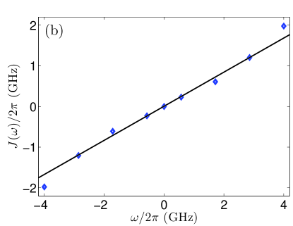
Figure 2: (Color online) (a) Measured MRT rate as a function of $\epsilon$ at $T=21$ mK and $\Phi^{x}_{\rm{ccjj}}/\Phi_{0}=-0.6344$. The dashed curve is calculated using Eq. (4) with $W/h=0.47$ GHz. The solid curve is calculated using Eq. (12) with $W/h=0.47$ GHz and $\eta=0.41$. (b) $J(\omega)$ extracted from the experimental data using Eq. (10). The solid line is $J(\omega)=0.41\omega$.

The basic MRT rate measurement technique has been described elsewhere R. Harris et al. (2008). Figure 2(a) shows example rate measurements versus $\epsilon$. The lowest energy MRT peak is very well separated from the next lowest resonant tunneling peak, which occurs at $\epsilon/h\sim 13$ GHz above the first peak (see process $\Gamma_{0\rightarrow 2}$ depicted in Fig. 1(a)). For the half-decade in $\Gamma(\epsilon)$ near the peak, the Gaussian lineshape (4) is a reasonable description of the data. To describe the resonant peak away from its maximum, we allowed for finite $S_{HF}(\omega)$ and extracted $J(\omega)$ from the data using Eq. (10). The results, plotted in Fig. 2(b), agree very well with a straight line with slope $\eta{=}\,0.41$ up to $|\omega/2\pi|{\approx}\,4$ GHz, the highest frequency for which we collected $\Gamma(\epsilon)$. Linearity of $J(\omega)$ implies an ohmic environment. The theoretical lineshape calculated via Eq. (12) using $\eta{=}\,0.41$ is in excellent agreement with the experimental data [solid curve in Fig. 2(a)].

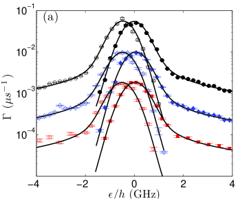
Figure 3: (Color online) Example measurements of MRT rate versus $\epsilon$ for (a) three different barrier heights ($\Phi^{x}_{\rm{ccjj}}/\Phi_{0}=-0.6344,-0.6355,-0.6365$ from top to bottom, respectively) at $T=21$ mK, and (b) a single barrier height, $\Phi^{x}_{\rm{ccjj}}/\Phi_{0}=-0.6344$, and three temperatures. The hollow (solid) symbols are $\Gamma_{0\rightarrow 1}(\Gamma_{1\rightarrow 0})$. The solid lines are a fit to Eq. (12).

Given the success of an ohmic model for $S_{HF}(\omega)$, we proceeded to directly fit a larger set of experimental data to Eq. (12). Figure 3(a) shows measurements of $\Gamma(\epsilon)$, both $\Gamma_{0\rightarrow 1}$ and $\Gamma_{1\rightarrow 0}$, for three different values of $\Phi^{x}_{\rm{ccjj}}$ ($\Phi^{x}_{\rm{ccjj}}/\Phi_{0}=-0.6344,-0.6355$ and $-0.6365$) with solid lines indicating fits to Eq. (12). We obtained fit values of $\Delta_{r}/h=3.15\pm 0.07,1.38\pm 0.08$ and $0.60\pm 0.04$ MHz from top to bottom, respectively. The extracted temperature was $T=21\pm 1$ mK, in agreement with thermometry mounted on the mixing chamber of the dilution refrigerator. The fit width $W/h=0.47\pm 0.02,0.47\pm 0.02,$ and $0.49\pm 0.02$ GHz from top to bottom, respectively. We obtained $\eta=0.41\pm 0.03,0.42\pm 0.03,0.425\pm 0.05$ from top to bottom, respectively.

We also performed MRT rate measurements at $\Phi^{x}_{\rm{ccjj}}{=}-0.6344\ \Phi_{0}$ for a range of chip temperatures from 21 to 38 mK. Figure 3(b) shows example measurements and fits for three temperatures. We monitored the chip temperature via refrigerator thermometry and confirmed it by measuring the qubit transition width as described in R. Harris et al. (2010). The temperatures extracted from the fit parameters used in Fig 3(b) match those reported by thermometry and those obtained via qubit transition width measurements. Fit values of $\eta$ and $W$ were relatively insensitive to chip temperature over the range probed in our experiments. We note that the $T$-independence of $W$ implies a $1/T$-dependence of the linear response of the low frequency environment (typical, for example, of a population of paramagnetic spins) R. Harris et al. (2008). In contrast, the $T$-independence of $\eta$ implies $T$-independence of the linear response of the high frequency environment, consistent with an ohmic environment. We observed a gradual increase of $\Delta_{r}/h$ with $T$: $\Delta_{r}/h=3.15\pm 0.07,3.45\pm 0.08,$ and $3.6\pm 0.1$ MHz for 21 mK, 30 mK and 38 mK, respectively. Only a fraction of this increase in $\Delta_{r}/h$ with $T$ can be accounted for by the renormalization of $\Delta$ in Eq. (12), given the best fit value of $\eta$. The rest may be due to the influence of the higher energy levels in the flux potential wells.

The dimensionless parameter $\eta$ characterizes the amplitude of the high frequency noise spectral density at a given $\Phi^{x}_{\rm{ccjj}}$, and therefore one particular persistent current $|I^{p}_{q}|$, for our devices. To move closer to a physical picture of the source of high frequency noise, we can relate $S_{HF}(\omega)$ to an effective flux noise $S_{\Phi}(\omega)$ by scaling the former by the persistent current at which the measurement was performed, $S_{\Phi}(\omega)=S_{HF}(\omega)/(2|I^{p}_{q}|)^{2}$.

The source of ohmic flux noise can be parameterized as an effective resistance $R_{s}$ shunting the qubit junctions. The noise spectral density would then be

$$S_{\Phi}(\omega)=\frac{2L_{q}^{2}}{R_{s}}{\frac{\hbar\omega}{1-e^{-\hbar\omega/k_{B}T}}}.$$ (13)

Using the measured qubit properties and the extracted $\eta~{}\approx~{}0.42$, we calculate an effective shunt resistance

$$R_{s}=\frac{8|I^{p}_{q}|^{2}L_{q}^{2}}{\hbar\eta}\sim 20\ \rm{k}\Omega.$$ (14)

Another potential source of ohmic noise could be external qubit flux bias leads, each of which can be modeled as an impedance $Z_{0}$ coupled to the qubit body with $M=2$ pH. Considering the bias coupled to the qubit body and using measured qubit properties and $\eta~{}\approx~{}0.42$, we calculate an effective impedance

$${\rm{Re}}(Z_{0})=\frac{8|I^{p}_{q}|^{2}M^{2}}{\hbar\eta}\sim 1\ \Omega.$$ (15)

Both of the ohmic sources hypothesized above predict impedances that are at least an order of magnitude smaller than expected (independent junction measurements suggest $R_{s}>500\ \rm{k}\Omega$; we estimate $Z_{0}\sim 25\ \Omega$), making the ultimate source of the high frequency environment uncertain. Generally, the amplitude of the high frequency noise should depend strongly on the details of the qubit wiring, junction size, and strength of coupling to bias leads depending on its source. Future measurements of this amplitude for a variety of qubits with a range of wiring and junction sizes will allow us to probe the ultimate source of this noise.

To summarize, we have developed and experimentally tested a method for extracting the high frequency noise spectral density $S_{HF}(\omega)$ from MRT rate measurements on flux qubits. Our experimental data are consistent with an ohmic spectral density up to $\omega/2\pi=4$ GHz. We have derived a theoretical expression for the MRT lineshape that includes both low and high frequency noise components. The resulting model fits the experimental data very well. In particular, this model explains tunneling rate measurements away the resonant peak, where the model without high frequency noise fails. Our method allows further exploration of high frequency noise in devices via its dependence on qubit geometry and fabrication details. A systematic study of a range of qubit designs will aid in ultimately understanding the origin of high frequency noise in superconducting qubits.

We acknowledge fruitful discussions with F. Cioata, P. Spear, E. Chapple, P. Chavez, C. Enderud, J. Hilton, C. Rich, G. Rose, M. Thom, S. Uchaikin, and B. Wilson.

References

- R. J. Schoelkopf et al. (2002) R. J. Schoelkopf et al., ArXiv Condensed Matter e-prints (2002), eprint arXiv:cond-mat/0210247.
- R. W. Simmonds et al. (2004) R. W. Simmonds et al., Phys. Rev. Lett. 93, 077003 (2004).
- J. M. Martinis et al. (2005) J. M. Martinis et al., Phys. Rev. Lett. 95, 210503 (2005).
- D. Bennett et al. (2009) D. Bennett et al., Quantum Information Processing 8, 217 (2009).
- McDermott (2009) R. McDermott, IEEE Transactions on Applied Superconductivity 19, 2 (2009).
- F. Yoshihara et al. (2006) F. Yoshihara et al., Phys. Rev. Lett. 97, 167001 (2006).
- R. C. Bialczak et al. (2007) R. C. Bialczak et al., Phys. Rev. Lett. 99, 187006 (2007).
- T. Lanting et al. (2009) T. Lanting et al., Phys. Rev. B 79, 060509 (2009).
- F. Yoshihara et al. (2010) F. Yoshihara et al., Phys. Rev. B 81, 132502 (2010).
- Rouse et al. (1995) R. Rouse, S. Han, and J. E. Lukens, Phys. Rev. Lett. 75, 1614 (1995).
- L. Thomas et al. (1996) L. Thomas et al., Nature (London) 383, 145 (1996).
- W. Zheng et al. (1998) W. Zheng et al., Solid State Communications 108, 839 (1998).
- Y. Bomze et al. (2009) Y. Bomze et al., Phys. Rev. B 79, 241402 (2009), eprint 1010.1527.
- Amin and Averin (2008) M. H. S. Amin and D. V. Averin, Phys. Rev. Lett. 100, 197001 (2008).
- R. Harris et al. (2010) R. Harris et al., Phys. Rev. B 81, 134510 (2010).
- T. Lanting et a. (2010) T. Lanting et a., Phys. Rev. B 82, 060512 (2010).
- R. Harris et al. (2008) R. Harris et al., Phys. Rev. Lett. 101, 117003 (2008).
- Amin and Brito (2009) M. H. S. Amin and F. Brito, Phys. Rev. B 80, 214302 (2009).
- Averin et al. (2000) D. V. Averin, J. R. Friedman, and J. E. Lukens, Phys. Rev. B 62, 11802 (2000).
- A. J. Leggett et al. (1987) A. J. Leggett et al., Rev. Mod. Phys. 59, 1 (1987).