Special Relativistic Magnetohydrodynamic Simulation of Two-Component Outflow Powered by Magnetic Explosion on Compact Stars

Abstract

The nonlinear dynamics of outflows driven by magnetic explosion on the surface of a compact star is investigated through special relativistic magnetohydrodynamic simulations. We adopt, as the initial equilibrium state, a spherical stellar object embedded in hydrostatic plasma which has a density $\rho(r)\propto r^{-\alpha}$ and is threaded by a dipole magnetic field. The injection of magnetic energy at the surface of compact star breaks the equilibrium and triggers a two-component outflow. At the early evolutionary stage, the magnetic pressure increases rapidly around the stellar surface, initiating a magnetically driven outflow. A strong forward shock driven outflow is then excited. The expansion velocity of the magnetically driven outflow is characterized by the Alfvén velocity on the stellar surface, and follows a simple scaling relation $v_{\rm mag}\propto{v_{\rm A}}^{1/2}$. When the initial density profile declines steeply with radius, the strong shock is accelerated self-similarly to relativistic velocity ahead of the magnetically driven component. We find that it evolves according to a self-similar relation $\Gamma_{\rm sh}\propto r_{\rm sh}$, where $\Gamma_{\rm sh}$ is the Lorentz factor of the plasma measured at the shock surface $r_{\rm sh}$. Purely hydrodynamic process would be responsible for the acceleration mechanism of the shock driven outflow. Our two-component outflow model, which is the natural outcome of the magnetic explosion, can provide a better understanding of the magnetic active phenomena on various magnetized compact stars.

1. Introduction

Plasma outflow from gravitationally bounded stellar objects is a universal phenomenon in astrophysics which is known to occur on a range of different spatial and energetic scales. Gaseous material containing synthesized elements and energy are supplied from the stellar source into the surrounding environment by these outflows. It is important to study the driving mechanism of the plasma outflow not only for the dynamical evolution of the stellar object itself, but also for the chemical and dynamical evolution of interstellar medium of galaxies.

The pioneering theory of stellar wind, which is the prototype of the astrophysical outflow, was developed by Parker (1958). It describes steadily accelerated plasma flow from a high-temperature corona into interstellar space. Weber & Devis (1967) extended Parker’s wind theory to include magnetic processes by modeling plasma outflows along open magnetic field line. In this model, the accelerated stellar wind collides with the interstellar medium and finally forms the shock wave.

The neutron star is known to have a relativistic plasma outflow, called as pulsar wind. The magnetosphere of rotating magnetized neutron star is filled with charged particles (Goldreich & Julian 1969; Sturrock 1971; Ruderman & Sutherland 1975). These charged particles flow out steadily along open magnetic field lines through the light cylinder where the co-rotation velocity coincides with the light speed. The plasma is accelerated to relativistic velocity by converting the rotational energy of the pulsar itself. The pulsar wind also interacts with the surrounding dense gas ejected from the progenitor stars and causes a termination shock (Kennel & Coroniti 1984).

Non-steady outflows exist universally in astrophysical systems. These should be seen as a more general class of outflows than the steady stellar wind. Of these non-steady flows, astrophysical jets are the most studied. Astrophysical jets are collimated bipolar outflows from central objects. It is believed that magneto-centrifugal and magnetic pressure forces are the most promising power for driving the collimation flow (Blandford & Payne 1982; Uchida & Shibata 1985; Shibata & Uchida1986). The magnetized jet from young stellar objects have a central role in prompting the collapse of molecular clouds and thus is essential for star formation (Machida et al. 2008). The super-massive black holes in active galactic nuclei also powers bipolar jets (Begelman et al. 1984; Bridle & Perley 1984). The most energetic event in the universe is the gamma-ray burst, and which is believed to be energized by ultra-relativistic bipolar flows formed when a massive stellar core collapses (Woosley 1993; MacFadyen & Woosley 1999).

The non-steady mass ejection event associated with solar flares is called ”coronal mass ejection (CME)” (Low 1996). The emergence of a twisted magnetic flux tube from below the solar surface, which supplies free energy to the system, triggers flares by magnetic reconnection (Ishii et al. 1998; Kurokawa et al. 2002; Magara 2003) and drives the associated CMEs (e.g., Mikic & Linker 1994; Shibata et al. 1995).

We can observe non-steady mass ejection phenomena analogous to the solar flare/CME activity in magnetar systems. The magnetar is a ultra-strongly magnetized neutron star with magnetic field of $10^{14}$–$10^{15}$ G (Duncan & Thompson 1992, Thompson & Duncan 1995; Harding & Lai 2006; Mereghetti 2008). The giant flare observed from the magnetar is surprisingly energetic ($10^{44}$–$10^{46}$ ergs) and is believed to be powered by releasing the enormous magnetic energy stored in the magnetar itself (Thompson & Duncan 1995; Lyutikov 2006; Masada et al. 2010). We note that the magnetar giant flare is also associated with an expanding ejecta (Cameron et al. 2005; Gaensler et al. 2005; Taylor et al. 2005).

While the energetic origin of the outflow is different in the various astrophysical systems, there is a characteristic common to all outflow phenomena. The magnetohydrodynamic (MHD) processes play a role in powering and regulating the outflow. It has been a central issue in the study of the astrophysical outflow to specify the MHD process which controls the outflow dynamics (Hayashi et al. 1996; Beskin & Nokhrina 2006; Spruit 2010). Nevertheless, the physical property and the acceleration mechanism of the outflow powered by the magnetic energy released from the compact stars have not yet been studied sufficiently (e.g., Komissarov & Lyubarsky 2004; Komissarov 2006; Takahashi et al. 2009).

This paper focuses on the outflow powered by a magnetic explosion on a compact star, such as neutron star. We investigate its nonlinear dynamics using 2.5-dimensional special relativistic MHD simulations. The purpose of this paper is to reveal the characteristics of the outflow which expands from the surface of the compact star into the surrounding medium. The relativistic effect on the physical properties of the outflow is a special interest of this work because such outflow should be easily accelerated to relativistic velocity.

This paper opens with descriptions of the numerical model in § 2. The numerical results of our relativistic MHD simulation are presented in § 3. The self-similar property of the outflow is studied in more detail using one-dimensional hydrodynamic simulation in § 4. In § 5, the characteristics and potential application of our outflow model are discussed. Finally, we summarize our findings in § 6.

2. Numerical Model

2.1. Governing Equations

We solve the special relativistic magnetohydrodynamic (SRMHD) equations in an axisymmetric spherical polar coordinate system ($r$, $\theta$, $\phi$). The fluid velocity $\mathbb{v}$, electric field $\mathbb{E}$ and magnetic field $\mathbb{B}$ in the system have three components while their derivatives in the $\phi$-direction are assumed to be zero. We adopt, as the equation of state for the surrounding medium, the ideal gas law with a ratio of the specific heats $\gamma=4/3$. For simplicity all the dissipative and radiative effects are ignored. The basic equations are then

$$\frac{\partial D}{\partial t} + \nabla\cdot(D\mathbb{v})=0\;,$$ (1)

$$\frac{\partial\mathbb{R}}{\partial t}+\nabla\cdot\Biggl{[}\biggl{(}P + \frac{B^{2}+E^{2}}{8\pi}\biggr{)}\mathbb{I}$$

$$+\Gamma^{2}(e+P)\frac{\mathbb{v}\mathbb{v}}{c^{2}} - \frac{\mathbb{B}\mathbb{B}+\mathbb{E}\mathbb{E}}{4\pi}\Biggr{]}=\rho\mathbb{g}\;,$$ (2)

$$\frac{\partial\epsilon}{\partial t} + \mathbb{\nabla}\cdot\mathbb{R}c^{2}=\rho\mathbb{v}\cdot\mathbb{g}\;,$$ (3)

$$\frac{\partial\mathbb{B}}{\partial t}-\nabla\times( \mathbb{v} \times\mathbb{B})=0\;,$$ (4)

$$\mathbb{E}= - \frac{\mathbb{v}\times\mathbb{B}}{c}\>,$$ (5)

where

$$D \equiv \Gamma\rho\;,$$ (6)

$$\mathbb{R}\equiv\Gamma^{2}(e+ P )\frac{\mathbb{v}}{c^{2}}+\frac{\mathbb{E}\times\mathbb{B}}{4\pi c}\;,$$ (7)

$$\epsilon\equiv\Gamma^{2}(e+P)- P +\frac{B^{2}+E^{2}}{8\pi}.$$ (8)

Here $\Gamma\equiv[1-(v/c)^{2}]^{-1/2}$ is the Lorentz factor, and $e\equiv\rho c^{2}+P/(\gamma-1)$ is the internal energy. In Newtonian gravity $\mathbb{g}$, we do not take account of the relativistic correction on the gravitational force because it should be negligible in the neutron star system. D, $\mathbb{R}$ and $\epsilon$ denote the density, the momentum density and the energy density measured in the laboratory frame respectively. The other symbols have their usual meanings.

We use the HLL scheme (Harten et al. 1983) to solve the SRMHD equations in the same manner as Leismann et al. (2005). The numerical flux across the cell interface is evaluated using the characteristic velocity of the fast magneto-sonic wave obtained from the physical variables in left and right adjacent cells of the interface. The primitive variables are calculated from the conservative variables following the method of Del Zanna et al. (2003). We use a MUSCL-type interpolation method to attain second order accuracy in space, and Constrained Transport method to guarantee a divergence free magnetic field (Evans & Hawley 1988).

2.2. Initial Setting of Numerical Model

For our initial conditions, we consider a hydrostatic gas surrounding a central compact star. A dipole magnetic field anchored in the central star threads the external gaseous plasma, and is given by

$$B_{r} = \frac{2B_{0}{R_{*}}^{3}cos\theta}{r^{3}}\;,$$ (9)

$$B_{\theta} = \frac{B_{0}{R_{*}}^{3}sin\theta}{r^{3}}\;,$$ (10)

$$B_{\phi} = 0.$$ (11)

where $B_{0}$ and $R_{*}$ are the field strength at the equatorial plane on the stellar surface and the radius of the central star respectively. We assume that the temperature of the surrounding medium is inversely proportional to the distance from the centroid of the star

$$T=T_{0}\biggl{(}\frac{r}{R_{*}}\biggr{)}^{-1}\;,$$ (12)

where $T_{0}$ is the reference temperature of the surrounding gas on the surface of the central star. Then the spatial distribution of the gas density and pressure in hydrostatic equilibrium are

$$\rho = \rho_{0}\biggl{(}\frac{r}{R_{*}}\biggr{)}^{-\alpha}\;,$$ (13)

$$P = P_{0}\biggl{(}\frac{r}{R_{*}}\biggr{)}^{-(\alpha+1)}\;,$$ (14)

where

$$\alpha \equiv \frac{G\rho_{0}M_{*}}{P_{0}R_{*}}-1\;.$$ (15)

Here $\rho_{0}$ and $P_{0}$ are the reference density and pressure of the surrounding gas on the central star, and $M_{*}$ is the central stellar mass. The parameter $\alpha$ denotes the power-law index of the initial density profile.

The convectively stable condition for the surrounding gas is

$$\frac{ds}{dr}>0\;,$$ (16)

where $s$ is the entropy (Kippenhahn & Weigert 1990). When adopting equations (12)–(15), this can be reduced to

$$\alpha>\frac{1}{\gamma-1}=3\;.$$ (17)

We should set the parameter $\alpha$ to be larger than $3$ in our calculations for maintaining the surrounding plasma being convectively stable. On the other hand, models with $\alpha>7.25$ can not be solved using our simulation code because the physical variables become too small to be resolved in the calculation domain. The parameter $\alpha$ surveyed in the following is thus restricted to the range between $3.0$ and $7.25$.

The ratio between the mass and radius of the central star is a fundamental parameter which characterizes the system, and is fixed as $M_{*}/R_{*}=2.2\times 10^{27}\ {\rm g/cm}$. This is the typical value for the neutron star. All the numerical models we examined here are controlled by two non-dimensional parameters, which are the power-law index $\alpha$ of the hydrostatic surrounding medium and the plasma beta on the equatorial surface of the central star $\beta_{0}\equiv P_{0}/(B_{0}^{2}/8\pi)$.

As we show in § 3.2, the temporal evolution of the magnetically driven outflow is controlled by the initial Alfv́en velocity ($v_{\rm A}$). The larger value of initial plasma beta ($\propto v_{\rm A}^{-2}$) provides the slower evolution of the outflow, which is not appropriate for extensive parameter survey. In addition, the conservative MHD scheme used in our code is not good at solving the problem with small values of the initial plasma beta. Hence we survey the $\beta_{0}$-dependence of the outflow properties within the range $3.2<\beta_{0}<3.2\times 10^{3}$.

The relativistic representations of the sound speed and Alfvén velocity $v_{\rm s,0}^{\;R}$ and $v_{\rm A,0}^{\;R}$ are, at the equatorial surface of the central star,

$$v_{\rm s,0}^{\;R} = \frac{v_{\rm s,0}}{\sqrt{1+\xi/(\alpha+1)}}$$ (18)

$$\simeq v_{\rm s,0}\;\biggl{(}\because\ \ \xi\equiv\frac{\gamma}{\gamma-1}\frac{GM_{\rm*}}{R_{\rm*}c^{2}}\simeq 0.65\biggr{)}\;,$$

$$v_{\rm A,0}^{\;R} = \frac{v_{\rm A,0}}{\sqrt{1+[1+2(\gamma-1)/(\gamma\beta_{0})][\xi/(\alpha+1)]}}$$ (19)

$$\simeq v_{\rm A,0}\;,$$

where

$$v_{\rm s,0}=\sqrt{\frac{\gamma P_{0}}{\rho_{0}}}\;,\ \ \ \ \ v_{\rm A,0}=\frac{B_{0}}{\sqrt{4\pi\rho_{0}}}\;.$$ (20)

Here $v_{s,0}$ and $v_{{\rm A},0}$ are the sound speed and Alfvén velocity at the equatorial surface of the central star in the non-relativistic limit. Since the parameter $\alpha$ varies from $3.0$ to $7.25$ and $\beta_{0}$ varies from $3.2$ to $3.2\times 10^{3}$ in our models, the relativistic representations of the sound and Alfvén velocities can be well approximated by their non-relativistic forms as stated above. Using description (15), the sound and Alfvén velocities are

$$v_{\rm s,0}/c = 0.48(\alpha+1)^{-1/2}\;,$$ (21)

$$v_{\rm A,0}/c = 0.32(\alpha+1)^{-1/2}\biggl{(}\frac{\beta_{0}}{3.2}\biggr{)}^{-1/2}\;.$$ (22)

In the following, we mainly use the non-relativistic form of the sound and Alfvén velocity for convenience. The normalization units in length, velocity and time are chosen for all the models as radius of the central star $R_{*}$, light speed $c$, and the light crossing time $\tau=R_{*}/c$.

2.3. Boundary Condition and Numerical Grid

The stress-free condition is applied to the outer radial boundary located at $r=200R_{*}$. At the inner radial boundary ($r=R_{*}$), we impose the condition that the physical variables except $v_{\phi}$ and $B_{\phi}$ are fixed to be time-independent, that is, $\partial/\partial t|_{r=R_{*}}=0$. The radial and latitudinal velocities of the gas $v_{r}$ and $v_{\theta}$ vanish at the stellar surface. The gas density, the gas pressure and the poloidal field strength at the stellar surface are consistently determined from equations (9)-(14). The stress-free condition is adopted at the inner boundary only for the toroidal magnetic field $B_{\phi}$.

The shearing motion at the inner boundary regulates the energy injection into the calculation domain. On the equatorial surface, we impose a shear flow with the longitudinal velocity

$$v_{\phi}(R_{*},\theta,t)=\Delta v_{\phi}(t)\Theta\exp[(1-{\Theta}^{4})/4]\;,$$ (23)

where $\Theta=(\theta-\pi/2)/\Delta\theta_{\rm peak}$ (see Mikic & Linker 1994). $\Delta\theta_{\rm peak}$ controls the latitudinal width within which the shearing motion is operated, and is fixed as $\pi/9$ in the following.

We investigate two different energy injection patterns. In both cases, the shearing velocity $\Delta v_{\phi}(t)$ increases linearly from zero to $0.1c$ between $t=0$ and $10\tau$ and is held at constant velocity $0.1c$ until $t=20\tau$. After $t=20\tau$, the velocity of the shearing motion is kept constant at $0.1c$ in case A, and is terminated suddenly in case B.

The amplitude of the shearing velocity is an important parameter which controls the outflow dynamics, and should be widely surveyed. However, we focus only on the typical case with the fixed shearing velocity of $0.1c$ in this paper. In this case, the shearing motion supplies the magnetic energy which is roughly comparable to the thermal energy of the system. The dependence of the outflow dynamics on the initial field strength and the density profile of the surrounding gas is our interest in this paper. We will study the impact of the shearing velocity on the outflow dynamics in the separate paper.

The polar angle of the calculation domain is uniformly divided into $\Delta\theta=\pi/90$. A nonuniform grid is adopted in the radial direction. The radial grid size $\Delta r$ gradually increases from $0.036R_{*}$ (at $r=R_{*}$) to $0.2R_{*}$ (at $r=5R_{*}$), and is fixed as $0.2R_{*}$ outside $r=5R_{*}$. The largest grid size $\Delta r=0.2R_{*}$ is empirically determined to correctly capture the the sharp relativistic shock which propagates through the outer calculation domain. The number of the grid points is set as $1024$ in the radial and $90$ in the $\theta$ direction for all the models.

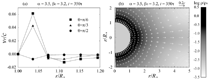
Figure 1.— Panel (a): the radial profile of the radial velocity for the model where $\alpha=3.5,\beta_{0}=3.2$ at the steady state on around the inner boundary region. The filled square, triangle and circle represent the profiles at the different polar angles $\theta=\pi/6$, $\pi/3$, and $\pi/2$ (along the equatorial plane), respectively. Panel (b): the density distribution (log scale) and poloidal velocity vector near the inner boundary on the meridional plane at the steady state. The density is normalized by its inner boundary value. The orientation and length of each arrow denote the direction and magnitude of the poloidal velocity vector at each meridian point.

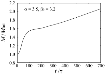
Figure 2.— The temporal evolution of the total mass contained in the calculation domain for the model where $\alpha=3.5,\beta_{0}=3.2$. The vertical axis is normalized by the initial total mass of the plasma distributed in the entire domain.

2.4. Dynamical Effects of the Boundary Condition

The shearing motion imposed on the equatorial surface of the compact star generates the toroidal magnetic field by stretching the initial dipole field. The kinetic energy of the shearing motion is then immediately converted to magnetic energy. The magnetic energy amplified above the stellar surface initiates the dynamical evolution of the system. While the shearing motion is added artificially to break the initial equilibrium of the system, it is physically modeling the supply of the magnetic helicity and energy from the stellar interior into the magnetosphere, like as the flux emergence in the sun.

In the solar flare/CME process, the emergence of the tightly twisted magnetic flux plays a triggering role in breaking the equilibrium of the corona (Ishii et al. 1998; Kurokawa et al. 2002; Magara 2003). We use the shearing motion instead of the flux emergence for the sun as the process modeling energy and helicity injection in our calculations, because actual energy and helicity injection processes are still veiled in mystery in the context of compact stars.

Since the inner boundary condition in our models is mathematical over-determined (see Bogovalov 1997), there exists a discontinuity in the radial velocity at around the stellar surface in our calculations. Figure 1a depicts the radial profile of the radial velocity of the model where $\alpha=3.5$ and $\beta_{0}=3.2$ as a reference. Here we focus on the inner boundary region ($1\leq r/R_{*}\leq$1.2) and the time-steady state of $t=350\tau$. The filled square, triangle and circle represent the radial velocity profiles at different polar angles $\theta=\pi/6$, $\pi/3$, and $\pi/2$ respectively. This addresses that there exists a velocity discontinuity near the inner boundary. In addition, the discontinuity at around the high latitude stellar surface has a larger amplitude than that around the equatorial region where the outflow is mainly accelerated in our models as shown in § 3.

Figure 1b shows the meridional distribution of the density and poloidal velocity near the inner boundary at the steady state of the model same as Figure 1a. The orientation and length of each arrow denote the direction and magnitude of the poloidal velocity vector at each meridian point. The grey contour is a logarithmic representation of the density normalized by its inner boundary value. The radial flow across the inner boundary is induced especially at around the high latitude stellar surface although the radial velocity is set to be zero at the inner boundary. This induced outgoing radial flow supplies the plasma into the calculation domain.

The temporal evolution of the total mass contained in the calculation domain is presented in Figure 2 in the same model. The vertical axis is normalized by the initial total mass of the plasma distributed in the entire domain. The total mass in the system increases with time due to the mass inflow from the inner boundary region. The mass injection rate is roughly $10^{-2}\;M_{\rm ini}/\tau$ at the initial evolutionary stage until $100\tau$, but $10^{-3}\;M_{\rm ini}/\tau$ at the steady state after $200\tau$.

Since the density of the plasma near the stellar surface is maintained at close to the initial value by the mass inflow across the inner boundary as shown in Figure 1b, the Alfv́en and sound velocity ($\propto\rho^{-1/2}$) are not relativistic there and an order of $0.1c$ at the steady state. The radial velocity is less than $0.01c$ when focusing on the equatorial region where the magnetic energy is strongly amplified and the outflow is energized, while its latitudinally-averaged value is roughly $0.05c$.

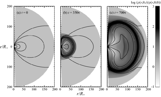
Figure 3.— The time evolution of the density distribution (log scale) and magnetic field lines in the meridional plane for the model where $\alpha=3.5$ and $\beta_{0}=3.2$. The density is normalized by its initial value: $\rho(r,\theta,t)/\rho(r,\theta,0)$. The left, middle and right panels are corresponding to those in $t/\tau=0$, $350$, and $700$ respectively.

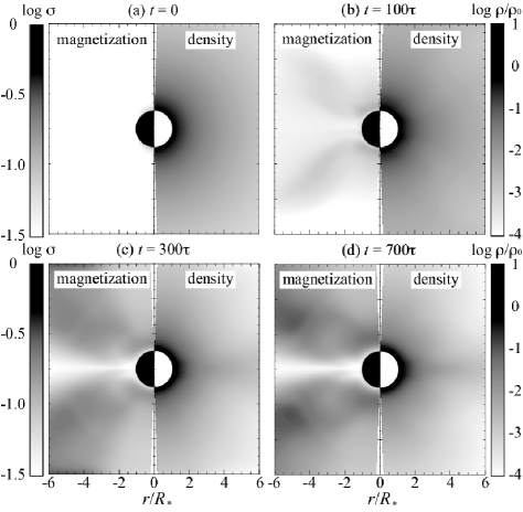
Figure 4.— The temporal evolution of the magnetization ($\sigma\equiv B^{2}/4\pi\Gamma^{2}\rho c^{2}$) and density on the meridian plane where $\alpha=3.5$ and $\beta_{0}=3.2$ at the times (a) $t=0$, (b) $t=100\tau$, (c) $t=300\tau$ and (d) $t=700\tau$ respectively. The density is normalized by the reference density of the surrounding gas on the central star. The contours are filled by a logarithmic gray scale. The region occupied by the central compact object is filled by black and white in the left and right parts of each panel.

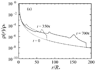
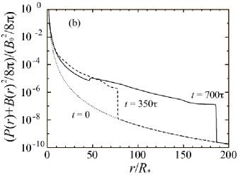
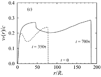
Figure 5.— Panels (a) the density, (b) the total pressure (thermal + magnetic pressures), and (c) the radial velocity on equatorial plane as a function of the normalized radius $r/R_{*}$ where $\alpha=3.5$ and $\beta_{0}=3.2$. Dotted, dashed, and solid lines are corresponding to those in t/$\tau$ =0, 350 and 700, respectively.

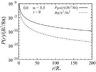
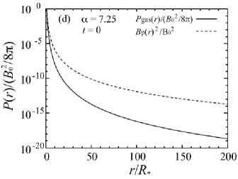
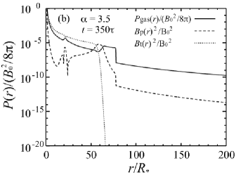
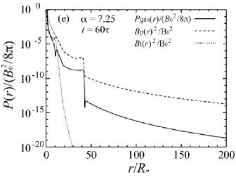
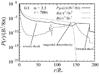
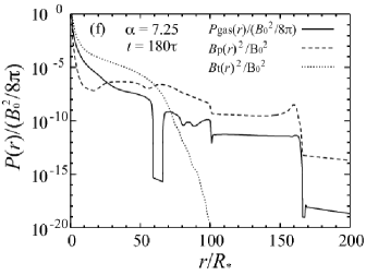
Figure 6.— Left column: temporal evolution of the radial distribution of the gas and magnetic pressures where $\alpha=3.5$ and $\beta_{0}=3.2$ at the times (a) $t=0$, (b) $t=350\tau$ and (c) $t=700\tau$ respectively. Right column: the model $\alpha=7.25$ and $\beta_{0}=3.2$. Note that all pressure components are measured on the equatorial plane. The magnetic pressure is divided into two parts in these panels, one is the contribution from toroidal magnetic fields $B_{t}$, and the another is that from the poloidal fields $B_{p}$.

3. Results

3.1. Temporal evolution of a fiducial model

We show the dynamical evolution of the outflow in a fiducial model ($\alpha=3.5$ and $\beta_{0}=3.2$). The case with continuous shearing motion (case A) is investigated here.

Figure 3 demonstrates the temporal evolution of the expanding outflow. The density and the magnetic field lines projected on the meridional plane are shown at the time (a) $t=0$, (b) $350\tau$ and (c) $700\tau$ respectively. Note that the grey contour is a logarithmic representation of the density normalized by its initial value.

The magnetic pressure resulted from the toroidal magnetic field, which is generated by the shearing motion around the stellar equatorial surface, initiates and accelerates the quasi-spherical outflow. The driven outflow is strongly magnetized, in which the magnetic pressure composed mainly of the contribution for the generated toroidal field dominates the gas pressure, and carries dense plasma away from the central star.

In the equatorial region where the magnetized outflow is energized, it is natural from the physical perspective to consider that the magnetization parameter ($\sigma\equiv B^{2}/4\pi\Gamma^{2}\rho c^{2}$) grows due to both the mass ejection and the continuous injection of the magnetic energy. However, the magnetization parameter near the stellar surface is maintained at a lower value than unity during the computing time as shown in Figure 4.

In this figure, the spatial distribution of the magnetization parameter (left) and density (right) are demonstrated by the logarithmic grey scale on the meridian plane. Different panels are corresponding to the different evolutionary phases (a) $t=0$, (b) $100\tau$, (c) $300\tau$ and (d) $700\tau$ respectively. The region occupied by the central star is filled by black and white in the left and right parts of each panel. The magnetization $\sigma$ near the stellar surface is less than unity. The mass inflow from the inner boundary region plays a role in reducing the magnetization parameter to less than unity.

Although the magnetic energy is strongly amplified and the outflow carries a large portion of the gas around the equatorial region, the rapid amplification of the magnetization parameter is prevented because the dense plasma maintained above the high-latitude stellar surface is continuously supplied into the equatorial region. This is the reason why the magnetization parameter $\sigma$ in the near surface region is less than unity at all the latitude during the computing time.

Figure 5 denotes the radial distributions of the (a) density, (b) total pressure (thermal + magnetic pressures) and (c) radial velocity along the equatorial plane ($\theta=\pi/2$). The dotted, dashed and solid lines represent the cases $t=0$, $350\tau$ and $700\tau$ of Figure 3 respectively. Note that the vertical axis is normalized by its reference value in each plot.

It is found that a strong forward shock is formed and expands supersonically into the surrounding medium. The shock powered by the magnetized outflow is accelerated to sub-relativistic velocity $\simeq 0.3c$. Behind the forward shock surface (around $50R_{\rm*}$ when $t=700\tau$), a reverse shock is excited and propagates through the shocked medium.

The time evolution of the gas and magnetic pressures are shown in Figure 6. The left column is of the case being discussed in this section. The top, middle and bottom panels correspond to phases (a) $t=0$, (b) $350\tau$, and (c) $700\tau$ in the fiducial model. In each panel, the solid line indicates the gas pressure, dotted and dashed lines are the magnetic pressure due to the poloidal and toroidal magnetic field respectively. The normalization of each curve is the initial magnetic pressure at the equatorial surface of the central star, that is ${B_{0}}^{2}/8\pi$.

In Figure 6c, we find a tangential discontinuity created behind the propagating forward shock. The magnetic pressure provided by the toroidal magnetic field becomes predominant behind the discontinuity. In contrast, the gas pressure dominates the magnetic pressure between the discontinuity and the shock surface throughout the evolution of the system, except for a transition region near the discontinuity.

3.2. Magnetically Driven Outflow

The physical properties of the magnetically driven outflow are examined through changing the $\alpha$-parameter that controls the density profile. We anticipate that the magnetically driven outflow velocity $v_{\rm mag}$ is characterized by the strength of the initial dipole field which is the seed of the predominantly toroidal field behind the tangential discontinuity. The relation between the velocity of the magnetically driven outflow and the initial field strength is elucidated here.

Figure 7 shows the outflow velocity $v_{\rm mag}$ in relation to the initial Alfvén velocity at the equatorial surface of the central star ($v_{\rm A,0}$) for the models $\alpha=3.5$, $4.5$, $5.5$, $6.5$, and $7.0$ respectively. The initial Alfvén velocity is the representative of the seed field strength and varies from $1.1\times 10^{-3}c$ to $0.15c$ when changing the size of $\alpha$ and $\beta$. The velocity is measured when the head of the magnetically driven outflow reaches $r=70R_{*}$.

The velocity of the magnetically driven outflow increases with the initial Alfvén velocity. The logarithmic fitting of the data provides the power law dependence between them as summarized in Table 1, where $\sigma\equiv{\rm d}\ln v_{\rm mag}/{\rm d}\ln v_{\rm A,0}$ denotes the power law index. The index $\sigma$ is nearly constant for all the models, that is $\sigma\simeq 0.5$. The dynamical evolution of the magnetically driven outflow thus follows a simple scaling relation, $v_{\rm mag}\propto{v_{\rm A,0}}^{1/2}$.

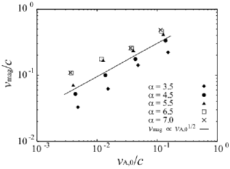
Figure 7.— The relation between the Alfvén velocity at the equatorial surface and the velocity of the tangential discontinuity measured at $r=70R_{*}$ when $\alpha=3.5$, $4.5$, $5.5$, $6.5$, and $7.0$. There is a simple scaling relation between these two values, $v_{\rm mag}\propto{v_{\rm A,0}}^{1/2}$.

Table 1Indices of a simple relation between the magnetically driven outflow velocity at tangential discontinuity surface and the initial Alfvén velocity at the equatorial surface of the central star when the power law index $\alpha$ of the initial density profile varies. The relation is $v_{\rm mag}\propto{v_{\rm A,0}}^{\sigma}$.

$\alpha$	3.5	4.5	5.5	6.5	7.0
$\sigma$	0.51	0.54	0.45	0.44	0.48

To draw a qualitative physical picture which is accountable for this scaling relation, we focus on two balancing equations. For simplicity, we reduce the governing equations (1)–(8) to their non-relativistic forms because the outflow velocity of interest here is sufficiently slower than the light speed. The numerical results address that in the steady state, the strength of the toroidal field behind the tangential discontinuity does not change significantly in time. Hence the radial advective loss of the toroidal field should approximately counterbalance the generation of the toroidal field by shearing motion at around the stellar surface. The azimuthal component of the induction equation can be simplified, at the steady state,

$$\frac{\partial B_{\phi}}{\partial t}=[\nabla\times(\boldsymbol{v}\times\boldsymbol{B})]_{\phi}$$

$$\leftrightarrow 0\simeq\frac{B_{0}\Delta v_{\phi}}{L}-\frac{B_{\phi\rm,amp}v_{r\rm,adv}}{R_{*}}\;,$$ (24)

where $B_{\phi,\rm amp}$ is the typical strength of the toroidal field in the region where it is strongly amplified and $v_{r,\rm adv}$ is the mean radial advection velocity there. The first term on the right hand side of equation (24) represents the generation of the toroidal field by the shearing motion within typical latitudinal width $L$, which is replaced using $L\simeq R_{*}\Delta\theta_{\rm peak}$ in the following. The second term shows the advective loss of the toroidal field with the mean radial velocity $v_{r,\rm adv}$. This yields the mean toroidal field in the steady state,

$$B_{\phi\rm,amp}\simeq\biggl{(}\frac{1}{\Delta\theta_{\rm peak}}\biggr{)}\biggl{(}\frac{\Delta v_{\phi}}{v_{r,\rm adv}}\biggr{)}B_{0}\;.$$ (25)

Our numerical results suggest that the magnetically driven outflow is mainly accelerated in the near-surface region where the toroidal field is strongly amplified as shown in Figure 6c and  7c. The velocity of the magnetized outflow does not change drastically in the region beyond the radius $r\simeq 10R_{*}$. This would address that large portion of the kinetic energy of the outflow is gained through the conversion of the magnetic energy in the near-surface region of the compact star.

In the steady state, the total energy of the magnetically driven outflow should be conserved along the streamline, which is almost radial in our models. The specific kinetic energy of the outflow at an arbitrary radius, at which the energy conversion is almost terminated, is thus given by integrating the magnetic pressure gradient force along the radial streamline from the stellar surface $R_{*}$ to the arbitrary radius $r$,

$$\frac{1}{2}{v_{r}(r)}^{2}=-\int^{r}_{R_{*}}\frac{1}{\rho}\frac{\partial}{\partial r}\biggl{(}\frac{{B_{\phi}}^{2}}{8\pi}\biggr{)}\;{\rm d}r\;,$$ (26)

(see Appendix for details). Since the magnetized outflow is not accelerated dramatically after the termination of the energy conversion, its mean radial velocity $v_{\rm mag}$ can be substituted for the local value $v_{r}(r)$ in equation (26). This energy balance equation yields the typical velocity of the magnetized outflow as a function of the mean toroidal field $B_{\phi,{\rm amp}}$ and the mean density $\rho_{\rm amp}$ in the region where the toroidal field is strongly amplified and the outflow gains the kinetic energy,

$${v_{\rm mag}}\simeq\frac{B_{\phi,\rm amp}}{\sqrt{4\pi\rho_{\rm amp}}}\;.$$ (27)

As the outflow velocity does not change drastically in the region beyond the near-surface of the central star, the mean advection velocity $v_{r,{\rm adv}}$ appeared in equation (25) should be comparable to the typical velocity of the magnetically driven outflow, that is $v_{r,\rm adv}\simeq v_{\rm mag}.$ Then, by combining equations (27) with (25), we can provide

$$v_{\rm mag}\simeq{v_{\rm A,0}}^{1/2}{\Delta v_{\phi}}^{1/2}\Delta\theta_{\rm peak}^{-1/2}\left(\frac{\rho_{\rm amp}}{\rho_{0}}\right)^{-1/4}\;,$$ (28)

where the parameters $v_{\rm A,0}$, $\Delta v_{\phi}$, and $\Delta\theta_{\rm peak}$ are initially given and remained to be constants. The relation (28) obtained using an order of magnitude analysis here is shown by the solid line in Figure 7. The numerical results are well reproduced by this analytic scaling. It is noted again that two balancing equations, which are reduced from the induction and energy equations, account for the scaling relation.

The physical property of the magnetized outflow studied here is different from that found in the similar work on solar CME by Mikic & Linker (1994). This would be because, in their work, the shearing motion which models the energy injection in the solar flare/CME process is much slower than the Alfvén velocity in comparison with our models. The magnetic energy is gradually stored above the solar surface and is released abruptly in their CME models. In contrast, in our models, the magnetic energy is immediately converted to the kinetic energy without being stored. Although there is less information about the injection mechanism and supply rate of the magnetic energy in the compact star, we expect that the rapid injection of the magnetic energy into the magnetosphere might be the origin of giant flares and the associated mass ejection in the magnetar system. We apply our numerical model to the magnetar system in § 5.

3.3. Relativistic Self-Similar Shock

The second component of the outflow is the shock driven outflow which proceeds the magnetically driven component. We examine how the initial density profile of the surrounding gas affects the shock driven outflow. The plasma beta at the equatorial surface is fixed as $\beta_{0}=3.2$ here for simplicity.

Figure 8 shows the plasma velocity of the shock surface measured at the reference point $r=150R_{*}$ and $\theta=\pi/2$ as a function of the index $\alpha$ which controls the density profile. The vertical axis denotes $\Gamma_{150}-1$, where $\Gamma_{150}$ is the Lorentz factor defined by $[1-(v_{150}/c)^{2}]]^{-1/2}$, and $v_{150}$ is the plasma velocity of the shock at the reference point. The value $\Gamma-1$ measured in this figure is useful for treating both relativistic and non-relativistic flows simultaneously. When the flow velocity reaches the ultra-relativistic regime, it roughly provides the Lorentz factor itself, that is $\Gamma-1\simeq\Gamma$. In contrast, it is the indicator of the flow velocity also in the non-relativistic case $v\ll c$, that is $\Gamma-1\simeq(v/c)^{2}/2$. It is found that the shocked plasma is eventually accelerated to mildly relativistic velocity in the model $\alpha=7.25$. There is a correlation between the shock velocity and the index $\alpha$. The $\alpha$-dependence of the Lorentz factor changes at $\alpha\simeq 5$. These indicate that the density profile of the surrounding gas is key to reveal the acceleration mechanism of the forward shock in our model.

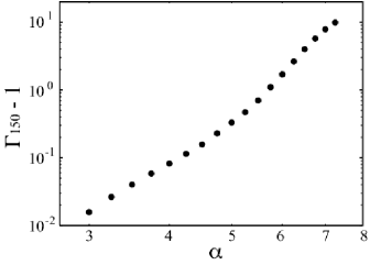
Figure 8.— The relation between the initial density profile of the surrounding medium ($\rho\propto r^{-\alpha}$) and the plasma velocity at the forward shock surface on the equatorial plane. Note that the velocity is measured when the shock surface reaches the equatorial radius $r=150R_{*}$. The vertical axis represents $\Gamma_{150}-1\equiv[1-(v_{150}/c)^{2}]^{-1/2}-1$ where $\Gamma_{150}$ and $v_{150}$ are the Lorentz factor and the plasma velocity at the shock surface when it reaches the fixed radius $r=150R_{*}$.

The right column in Figure 6 depicts the radial profile of pressure components along the equatorial plane at the time $t=0$, $60\tau$ and $180\tau$ for the model with the steep density profile ($\alpha=7.25$). The curves in panels (e), (f) and (g) have the same meaning as those for the model $\alpha=3.5$. The toroidal magnetic field generated by the shearing motion initially powers the magnetized component of the outflow. The forward shock is then excited and propagates through the surrounding medium in the same way as the model with $\alpha=3.5$.

There is a clear difference between the models with $\alpha=3.5$ and $\alpha=7.25$. That is the radial structure of the poloidal magnetic field. In the model with $\alpha=3.5$, the poloidal field is accumulated in front of the tangential discontinuity. The radial pressure gradient of the accumulated poloidal field seems to push the shock outward. This suggests that the shock wave is mainly accelerated by the magnetic pressure gradient force when the density profile moderately declines ($\alpha\lesssim 5$).

In contrast, there is no steep gradient in the poloidal magnetic field behind the shock in the model $\alpha=7.25$. Rather the propagation surface of the poloidal field coincides with the shock surface. This suggests that the excited shock wave propagates with the accumulated poloidal field when the density profile declines steeply ($\alpha\gtrsim 5$).

Temporal evolution of the radial velocity profile in the model $\alpha=7.25$ is presented along the equatorial plane in Figure 9. The vertical axis shows the Lorentz factor of the expanding gas. The horizontal axis is the equatorial radius. The dotted, dashed, dash-dotted, and dashed-two dotted curves correspond to the cases $t/\tau=80$, $120$, $160$ and $200$ respectively. The solid curve denotes the time trajectory of the Lorentz factor of the plasma velocity measured at the shock surface in the laboratory frame. The evolution of the relativistic shock has self-similar properties. The fitting of numerical data provides a scaling relation between the Lorentz factor $\Gamma_{\rm sh}$ and the equatorial radius $r_{\rm sh}$ at the shock surface

$$\Gamma_{\rm sh}\propto r_{\rm sh}\;.$$ (29)

The Lorentz factor of the plasma velocity at the shock surface increases linearly with the equatorial radius.

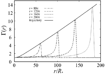
Figure 9.— The time evolution of the Lorentz factor of the expanding gas in the model with $\alpha=7.25$ and $\beta_{0}=3.2$. The dashed-two dotted, dot-dashed, dashed, and dotted curves indicate the models when $t/\tau=80$, $120$, $160$, and $200$ respectively. The solid line represents the time trajectory of the Lorentz factor of the fluid velocity at the shock surface measured in the laboratory frame. The scaling relation between the Lorentz factor $\Gamma_{\rm sh}$ and spherical radius $r_{\rm sh}$ of the shock surface in the laboratory frame is $\Gamma_{\rm sh}\propto r_{\rm sh}$. The relativistic shock evolves self-similarly.

Table 2 Indices of a relation between the Lorentz factor $\Gamma_{\rm sh}$ and the equatorial radius $r_{\rm sh}$ at the shock surface in the laboratory frame when the power law index $\alpha$ of the initial density profile varies. The relation is $\Gamma_{\rm sh}-1\propto{r_{\rm sh}}^{\delta}$.

$\alpha$	5.75	6.00	6.25	6.50	6.75	7.00	7.25
$\delta$	0.99	1.03	1.05	1.08	1.10	1.11	1.10

The other models with steep density gradient of $\alpha>5.5$ commonly yield a relation close to equation (29). Table 2 summarizes the power-law index $\delta$ when fitting the numerical models by a power-law relation $\Gamma_{\rm sh}-1\propto{r_{\rm sh}}^{\delta}$. It is important to stress that all the models which follow the scaling relation (29) have relativistic velocity, that is, $\Gamma_{150}>2$, at the reference point. The models with $\alpha\lesssim 5.5$ do not reach relativistic velocity at the reference point and not follow the relation (29). In § 5, the self-similar solution numerically discovered in our work is compared to the other analytic solutions, including the Blandford-McKee solution (Blandford & McKee 1976).

At the initial stage, the magnetic pressure, gas pressure, and gas density decrease with radius according to $r^{-6}$, $r^{-\alpha-1}$, and $r^{-\alpha}$ respectively [see equations (9)–(14)]. The plasma beta of the surrounding gas finally becomes smaller than unity for the model with $\alpha>5$ at a great distance even if it is larger than unity at the stellar surface. Moreover, the Alfv́en velocity of the initial surrounding gas increases with radius only for the model with $\alpha>6$. These imply that a critical point, at which the MHD effect on the outflow dynamics will be altered, might exist at around $\alpha=5$–$6$. Though the MHD effect might lead to some change in dynamics of the outflow, we will show that pure hydrodynamic mechanism can be responsible for the self-similar property of the shock by using a simplified one-dimensional hydrodynamic simulationl in § 4.

Our numerical models indicate that the two-component outflow would be a natural outcome of the magnetic explosion on a compact star. In the early stages, the magnetically driven outflow forms as a consequence of the rapidly rising magnetic pressure around the stellar surface. The magnetized outflow loaded with a dense circumstellar plasma expands, and finally excites a relativistic forward shock which has self-similar properties. Our two-component outflow model is applied to the magnetar system in § 5.2.

3.4. Impact of Energy Injection Pattern

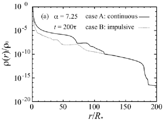
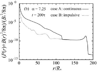
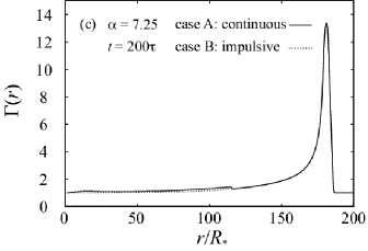
Figure 10.— The radial structures of the density, total pressure, and Lorentz factor of the plasma as a function of the normalized radius $r/R_{*}$ when $\alpha=7.25$, $\beta_{0}=3.2$, and $t=200\tau$. Case A, which is expressed by the solid line, corresponds to the case with continuous energy injection due to the shearing motion. Case B, which is depicted by the dashed line, indicates the case with impulsive energy injection. The shearing motion is terminated when $t=20\tau$ in Case B.

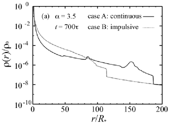
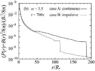
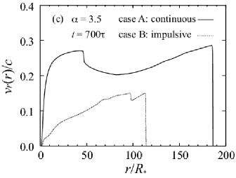
Figure 11.— Almost same as Fig 10, but where $\alpha=3.5$ and $t=700\tau$.

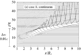
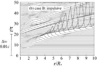
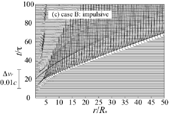
Figure 12.— Time-distance diagram for the time difference of the radial velocity $\Delta v_{r}(t,r)$ on the equatorial plane in the model $\alpha=7.25$ where $\Delta v_{r}(t,r)\equiv v_{r}(t,r)-v_{r}(t-\Delta t,r)$. Panel (a) corresponds to the continuous injection case (Case A), and (b) is the impulsive injection case (Case B). A wave which transmits the information for the termination of the energy injection is excited at $t=20\tau$ in the case B. Panel (c) just describes the long-time evolution of $\Delta v_{r}$ in case B. The information wave never reaches the propagating forward shock.

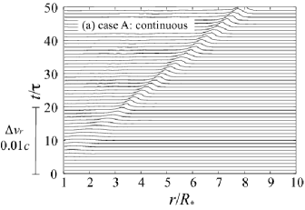
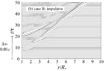
Figure 13.— Almost same as Fig 12, but when $\alpha=3.5$. In this model, the information wave can reach the propagating forward shock.

We clarify the impact of the energy injection pattern at the inner radial boundary on the evolution dynamics of the shock. As stated in § 2, we impose two different kinds of the energy injection pattern. These are the continuous injection case with the fixed shearing motion (case A) and the impulsive injection case in which we stop the shearing motion after $t=20\tau$ (case B). The plasma beta at the equator is fixed again as $\beta_{0}=3.2$.

Figure 10 depicts the radial distribution of the density, total pressure and Lorentz factor of the outflow measured at the equatorial plane for both cases when $t=200\tau$. The dashed and solid curves represent the cases A and B respectively. We choose the initial density profile with $\alpha=7.25$ for this figure. While there are differences in the structure of the magnetically driven outflow far behind the shock surface, we can not find any difference among two cases around the forward shock.

There is little difference in the structure around the shock between two cases when $\alpha>5.25$. However, for the model with $\alpha<5.25$, the different injection patterns provide different spatial structures of the shock as in the structures of the magnetically driven component. This can be verified by Figure 12, which shows the radial distribution of the density, total pressure and velocity in the fiducial model ($\alpha=3.5$) when $t=700\tau$ for the case A and case B. The curves have the same meanings as those in Figure 11.

We define a time difference value of the radial velocity on the equatorial plane $\Delta v_{r}$ as

$$\Delta v_{r}(t,r)\equiv v_{r}(t,r)-v_{r}(t-\Delta t,r)\;,$$ (30)

where $\Delta t$ denotes the numerical timestep. The time-distance diagram for the time difference value $\Delta v_{r}(t,r)$ is presented for the models $\alpha=7.25$ (Fig. 12) and $\alpha=3.5$ (Fig. 13). The vertical and horizontal axes denote the normalized time and radius. For specifying the temporal evolution of the outflow, the radial profiles of $\Delta v_{r}$ are plotted at every reference timestep on the time-distance plane. The reference timestep is set by the light crossing time $\tau=R_{*}/c$. Panel (a) corresponds to the case A and panel (b) is the case B in each figure.

In the case B, a wave is excited at $t=20\tau$ which corresponds to the termination time of the energy injection while it is not seen in the case A. This wave would thus transmit the information related to the energy injection pattern to the surrounding gas. We call this wave as ”information wave” hereafter. The information wave propagates through the surrounding medium, but never reaches the forward shock in the model $\alpha=7.25$ (see Figure 12b). This is because the propagation velocity of the forward shock is roughly light speed $c$ while that of the information wave is about $2c/3$.

Figure 12c is almost same as Figure 12b, but follows the long-term evolution of the time difference value. The excited information wave never interacts with the forward shock even when we follow its long-term evolution. This indicates that the inner boundary condition does not affect the evolution dynamics of the shock once it has been excited when the initial density profile is sufficiently steep ($\alpha>5.25$).

It would be natural to consider the effect of the termination time of the shearing motion on the shock dynamics in the impulsive injection case. There is actually a critical time $t_{\rm crit}$ beyond which the termination does not impact on the shock dynamics, that is $t_{\rm crit}\simeq 10\tau$. When stopping the shearing motion at the time before $t_{\rm crit}$, the information wave can catch up with the shock and change its dynamics even if the initial density profile is sufficiently steep. This is because the shearing velocity at the inner boundary $\Delta v_{\phi}(t)$ increases linearly from zero to $0.1c$ during $0\leq t\leq 10\tau$ (see § 2.3). The energy injection rate which determines the initial shock velocity becomes small if the shearing motion is terminated before $10\tau$. This is the reason why there exist the critical time. The shock dynamics does not change even if we stop the shearing motion at the time shorter than $20\tau$ as long as it continues longer than the critical time.

4. One-dimensional Hydrodynamic simulation

We examine the self-similar properties of the shock driven relativistic outflow in more detail using one-dimensional (1D) special relativistic hydrodynamic (HD) simulations, which enables us to study the numerical model in a wide parameter range. We specify here that a purely hydrodynamic process is responsible for the self-similar properties of the relativistic shock discovered in the two-dimensional (2D) MHD models.

4.1. Numerical Setting

We solve the 1D spherically symmetric system with $1024$ grid points radially using the same grid spacings as those in the 2D-MHD model. The MHD effects are fully ignored by dropping all the related terms in governing equations (1)-(8).

The numerical settings adopted in 1D-HD model are the same as those adopted in the 2D-MHD model except for the magnetic field. We consider a central compact star surround by a hydrostatic gas with the temperature, density, and pressure distributions described by equations (12)–(14). Since the sound velocity follows equation (21) with the index $\alpha$ varying from $3.0$ to $7.25$, it becomes non-relativistic ($\simeq 0.2c$) at the stellar surface. The symbols used in this section have the same meanings as those in the 2D-MHD model (see § 2.2).

The stress-free condition is applied to the outer boundary located at $r=200R_{*}$. At the inner boundary ($r=R_{*}$), we employ the condition that the physical variables except velocity are fixed. A plasma inflow is imposed on the inner boundary in 1D-HD models as a substitute for the shearing motion which is the energetic origin of the outflow in 2D-MHD models. This plasma flow excites the shock-driven outflow in the 1D models. The relation between the inflow velocity $v_{\rm in}$ and the injected energy flux $F_{\rm in}$ is given by $F_{\rm in}=\rho_{0}v_{\rm in}^{3}/2$. We study the properties of the shock driven outflow in the models with the inflow velocities $v_{\rm in}/c=1/10$, $1/30$, and $1/100$. Their dependence on the index $\alpha$ is also our interest in this section.

4.2. Properties of the Shock Driven Outflow

The continuous inflow powers a shock driven outflow. The cross symbol in Figure 14 shows the plasma velocity of the shock surface measured at $r=150R_{*}$ as a function of the power-law index $\alpha$. Note that the vertical axis is represented by $\Gamma_{150}-1$ like as Figure 8. As a reference, the 1D-HD model with $F_{\rm in}/F_{\rm ref}=1$ is focused, where $F_{\rm ref}$ is a reference value of the inflow energy flux which is equivalent to the model with $v_{\rm in}/c=1/10$. This model provides the almost same physical properties of the shock as those observed in the 2D-MHD model with a fixed shearing velocity $0.1c$. This is verified by Figure 14, in which the result of the 2D-MHD model is presented by the filled circle.

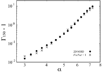
Figure 14.— The Lorentz factor of the shocked plasma velocity at $r=150R_{*}$ as a function of the density power-law index $\alpha$. The cross denotes the model calculated by one dimensional (1D) hydrodynamic simulations. The filled circle indicates the 2D special relativistic MHD model shown in Fig.8 again for the comparison. The meanings of vertical and horizontal axes are same as Fig.8. Note that $F_{\rm ref}$ is a reference value of the inflow energy flux which corresponds to the case with the inflow velocity $0.1c$.

The $\Gamma_{150}$-$\alpha$ relation in the 1D-HD model can reproduce that in the 2D-MHD model. The condition for the plasma velocity being relativistic in the 1D-HD model is also same as that in the 2D-MHD model, that is $\alpha>5.5$. These indicate that the shock driven outflow is accelerated to relativistic velocity by a purely hydrodynamic process even in the 2D-MHD model.

Figure 15 demonstrates the $\Gamma_{150}$-$\alpha$ relation for the models with different inflow energies. The cross, filled triangle, and filled diamond denote the models with $F_{\rm in}/F_{\rm ref}=1$, $1/27$, and $1/1000$ (that is, $v_{\rm in}/c=1/10$, $1/30$ and $1/100$) respectively. The Lorentz factor becomes higher for the model with the larger inflow flux. It is important to stress that the condition for the plasma velocity being relativistic ($\Gamma_{150}>2$) changes depending on the amount of the inflow flux. When setting the lower value of the $\alpha$ for providing the relativistic velocity as $\alpha_{\rm trans}$, we can find $\alpha_{\rm trans}=5.5$, $6.0$ and $7.0$ for the model with $F_{\rm in}/F_{\rm ref}=1$, $1/27$ and $1/1000$ respectively. The transition value $\alpha_{\rm trans}$, at which the shock velocity undergoes transition to the relativistic velocity, depends on the inflow flux. The larger inflow flux provides the smaller transition value.

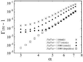
Figure 15.— $\Gamma_{150}$-$\alpha$ relations in the 1D steady energy injection model with $F_{\rm in}/F_{\rm ref}=1$, $1/27$, $1/1000$ and impulsive energy injection.

Note that the transition value $\alpha_{\rm trans}$ depends on the location where we measure the plasma velocity. We expect that the shock driven outflow is accelerated and finally reaches the relativistic velocity for all the continuous injection models as long as the initial density profile has a index $\alpha$ at least larger than $3$ (the smallest value for our parameter survey). With fixed inflow flux, the transition value $\alpha_{\rm trans}$ thus is expected to become smaller if the plasma velocity of the shock is measured at a more distant location. In other words, transition value is a function of the inflow flux and the location where the plasma velocity is measured.

Separately from the transition value, Figure 15 indicates that there exists a critical value of the index $\alpha$, at which the $\alpha$-dependence of the plasma velocity changes. The critical value $\alpha_{\rm crit}$ slightly shifts to the larger value with decreasing the inflow flux, that is $\alpha_{\rm crit}=4.0$, $4.25$ and $4.75$ for the models with $F_{\rm in}/F_{\rm ref}=1$, $1/27$ and $1/1000$ respectively. It is important to stress that the transition value $\alpha_{\rm trans}$ does not necessarily coincide with the critical value $\alpha_{\rm crit}$ according to the 1D-HD models, even though it has a coincidental match with the critical value in the 2D-MHD models, ($\alpha_{\rm trans}\simeq\alpha_{\rm crit}\simeq 5$ see § 3.3.). The degeneracy of these two values would be dissolved when the input energy is varied in the 2D MHD models.

To specify how the energy inflow pattern affects the dynamics, we examine the model with the impulsive inflow flux. The injected energy flux is fixed as $F_{\rm in}/F_{\rm ref}=1/1000$ here. The open squares in Figure 15 represent the 1D-HD models with the impulsive inflow. Note that the termination time, at which the energy injection is terminated, is fixed as $10\tau$ and is determined to provide the same total input energy as that in the 2D-MHD model with the impulsive injection pattern (case B). We find that the different inflow pattern provides a different $\alpha$-dependence of the Lorentz factor in the range $\alpha\lesssim\alpha_{\rm crit}$. In contrast, there is little difference in the $\alpha$-dependence of the Lorentz factor between two models when $\alpha\gtrsim\alpha_{\rm crit}$. These indicate that the energy inflow continuously injected into the system does not affect the acceleration of the shock wave as long as the initial density profile is sufficiently steep.

The evolution property of the shock is determined by the total amount of energy injected into the system in the duration till the termination time in the impulsive inflow cases. By contrast, in the continuous inflow cases, the shock is continuously accelerated without being terminated. The steady inflow cases thus provide the larger Lorentz factor than that for the impulsive inflow cases in the range $\alpha\lesssim\alpha_{\rm crit}$.

Figure 16 shows the time evolution of the shock velocity when $F_{\rm in}/F_{\rm ref}=1$ and $\alpha=7.25$ for the 1D-HD model. The axes have the same meanings as those of Figure 9. The different curves denote the shock profiles at the different phases $t/\tau=80$, $120$, $160$ and $200$ respectively. The solid line represents the trajectory of the Lorentz factor at the shock surface. The self-similar property of the relativistic shock in the 2D-MHD model is reproduced by the 1D-HD model. The self-similar evolution of the shock observed in the 1D-HD models also follows the relation $\Gamma_{\rm sh}\propto r_{\rm sh}$ as is obtained from the 2D-MHD models. These verify that a purely hydrodynamic process is responsible for the self-similar acceleration of the relativistic shock we found in the 2D MHD model.

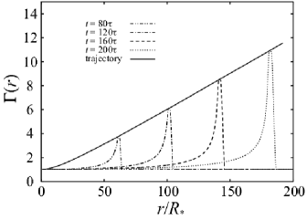
Figure 16.— The time evolution of the Lorentz factor in 1D hydrodynamic simulation where $\alpha=7.25$ and $v_{\rm in}=0.1c$. A solid line represents the time trajectory of the Lorentz factor at the shock surface measured in the laboratory frame. The meanings of vertical and horizontal axes are same as Fig.9.

5. Discussion

5.1. Comparison with Other Self-Similar Solutions

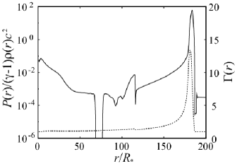
Figure 17.— The internal energy normalized by the rest mass energy and Lorentz factor of the plasma measured when $t=200\tau$ at the equatorial plane in the model where $\alpha=7.25$ and $\beta_{0}=3.2$. The left and right vertical axes show the internal energy and Lorentz factor respectively.

Piran et al. (1993) provides a detailed investigation of the dynamics of a fireball which is polluted by radiatively opaque plasma and whose internal energy is significantly greater than its rest mass energy. Because of its large opacity and huge internal energy, the extremely hot plasma expands adiabatically as a perfect fluid. The homogeneous fireball accelerates initially to a ultra-relativistic velocity and then coasts freely after converting all the internal energy into the kinetic energy.

The Lorentz factor of the expanding fireball $\Gamma_{\rm fb}$ follows the relation $\Gamma_{\rm fb}\propto r_{\rm fb}$ at the early acceleration stage where $r_{\rm fb}$ is its radius (Piran et al. 1993). This relation is seemingly the same as the relation describing the forward shock obtained from our numerical models. In our model, however, the shock propagates not at ultra-relativistic velocity rather at mildly relativistic velocity ($\Gamma_{\rm sh}\simeq 10$). In addition, unlike the fireball whose internal energy is significantly greater than the rest mass energy, the internal energy of the plasma behind the shock is less than the rest mass energy in our calculations, as is shown in Figure 17. Here we demonstrate the radial profile of the internal energy and Lorentz factor of the plasma measured at the equatorial plane when $t=200\tau$ for the model where $\alpha=7.25$ and $\beta_{0}=3.2$. The left vertical axis denotes the internal energy normalized by the rest mass energy and the left axis is the Lorentz factor. The physics which characterizes the self-similar acceleration of the relativistic shock we found are thus essentially different from that of the fireball model.

A spherical blast wave which expands supersonically into the surrounding medium is described well by a set of self-similar solutions. The Sedov-Taylor solution is the most famous of these, but only describes the case where the velocity is in a non-relativistic regime (Sedov 1959). When the released energy is much larger than the total rest mass energy of the explosion products and ambient gas, the velocity of the shock becomes relativistic. This type of shock also evolves self-similarly according to the Blandford-McKee solution at the ultra-relativistic limit (Blandford & McKee 1976).

When we consider the shock driven by impulsive energy injection in a gas with the density profile $\rho\propto r^{-\alpha}$, it is decelerated in the case $\alpha<3$ and accelerated for $\alpha>3$ (Shapiro 1979; Waxman & Shvarts 1993). The evolution of the shock follows the second type self-similar solution when the density of the surrounding gas declines steeply with radius (Waxman & Shvarts 1993; Best & Sari 2000). In the ultra-relativistic case, the Lorentz factor of the shock $\Gamma_{\rm sh}$ provides the relation $\Gamma_{\rm sh}\propto t^{-m/2}$ with $m=(3-2\sqrt{3})\alpha-4(5-3\sqrt{3})$, where $t$ is the time after the shock initiation (Best & Sari 2000). The index $-m/2\simeq 0.77$, $1.0$ and $1.23$ when the power law index $\alpha$ is $5$, $6$ and $7$ respectively.

The physical conditions required for the solutions presented above are similar to ours. However, these are not accountable for the outflow property we found in our study. This might be because our self-similar solution is more suited for describing the mildly relativistic shock which can not be treated by either non-relativistic or ultra-relativistic solutions. We analyze our self-similar solution in more detail by comparing the other solutions in a separate paper .

5.2. Application of Two-Component Outflow Model

As an application of our two-component outflow model to the realistic astrophysical system, we consider the magnetic explosion event in the magnetar system. Giant flares from soft gamma-ray repeaters are believed to be powered by the explosive release of the magnetic energy on the isolated magnetar (Thompson & Duncan 1995). It should be stressed that the giant flare on the magnetar is followed with an afterglow caused by the associated mass ejection event (Cameron et al. 2005; Gaensler et al.2005; Taylor et al. 2005).

Granot et al. (2006) diagnoses the observational properties of radio emitting ejecta observed in association with the giant flare on 2004 December 27 from SGR1806-20 (c.f., Taylor et al. 2005). It is suggested from their analysis that there is a possibility of the ejected matter containing two-types of components of sub-relativistic and mildly relativistic velocity. The origin and physics of the mass eruption event has not been determined although they give many clues to the model of the magnetar giant flare itself. Statistical analysis of giant flaring activity is needed for a better understanding of the magnetar.

Although the numerical setting adopted in our model does not correctly capture the realistic features of the plasma surrounding the magnetar system, our model creates an outflow with a mildly relativistic shock driven component and the subsequent sub-relativistic magnetically driven component loaded with dense plasma as a natural outcome of the magnetic explosion on a compact star.

On the basis of our numerical model, the observed giant flare, energized from the magnetic explosion on the magnetar, also powers the two-component outflow as is suggested by Granot et al. (2006). We aim to simulate the system of the compact star in the numerical setting more suited for the realistic magnetar system as part of our future work.

6. Summary

We investigate the nonlinear dynamics of the outflow powered by a magnetic explosion on a compact star using axisymmetric special relativistic MHD simulations. As an initial setting, we set a compact star embedded in the hydrostatic gaseous plasma which has a density $\rho(r)\propto r^{-\alpha}$ and is threaded by a dipole magnetic field. A longitudinal shearing motion is assumed around the equatorial surface, generating the azimuthal component of the magnetic field. Subsequent evolution was simulated numerically. Our main findings are summarized as follows.

1. Magnetic explosion on the surface of a compact star powers two-component outflow expanding into the static medium, i.e, magnetically driven and shock driven outflow. At the early evolutionary stage, the magnetic pressure due to the azimuthal component of the magnetic field initiates and drives a highly magnetized dense plasma outflow. Then the magnetically driven outflow excites a strong forward shock as the second outflow component.

2. The expanding velocity of the magnetically driven outflow depends on the Alfvén velocity at equatorial plane on the surface of the compact star $v_{\rm A,0}$ and follows a simple scaling relation $v_{\rm mag}\propto{v_{\rm A,0}}^{1/2}$. This scaling relation is accounted for in terms of coupling two balanced equations which are reduced from the induction equation and the energy equation.

3. When the initial density profile declines steeply with radius, the outflow-driven shock is accelerated self-similarly to relativistic velocity ahead of the magnetically driven outflow. The self-similar relation is $\Gamma_{\rm sh}\propto r_{\rm sh}$, where $\Gamma_{\rm sh}$ is the Lorentz factor of the fluid measured at the shock surface $r_{\rm sh}$. The pure hydrodynamic process is responsible for the acceleration of the shock driven outflow and for the self-similarity of the shocked wave.

Appendix A Derivation of the Energy Conservation Law along the Streamline

When the non-relativistic outflow is mainly polluted by the toroidal magnetic field, the radial outflow velocity should be controlled by the following equation of motion, in the spherical coordinate,

$$\rho\biggl{(}\frac{\partial v_{r}}{\partial t}+v_{r}\frac{\partial v_{r}}{\partial r}\biggr{)}=-\frac{\partial}{\partial r}\biggl{(}P+\frac{{B_{\phi}}^{2}}{8\pi}\biggr{)}-\frac{{B_{\phi}}^{2}}{4\pi r}-G\frac{\rho M_{*}}{r^{2}}\;.$$ (A1)

where all symbols have their usual meanings and the final term of this equation represents a gravitational force of the central object with mass $M_{*}$. Assuming the steady state, the radial velocity of the magnetically driven outflow should satisfy the steady state relation, which is reduced from equation (A1),

$$\frac{\partial}{\partial r}\biggl{(}\frac{1}{2}{v_{r}}^{2}\biggr{)}=-\frac{1}{\rho}\Biggl{[}\frac{\partial}{\partial r}\biggl{(}\frac{{B_{\phi}}^{2}}{8\pi}\biggr{)}+\frac{{B_{\phi}}^{2}}{4\pi r}\Biggr{]}\;,$$ (A2)

By integrating this equation along the radial streamline from the equatorial surface $R_{*}$ to the arbitrary radius $r$ and dropping the effect of the magnetic tension force on the dynamics, we can obtain the radial velocity $v_{r}(r)$ at the arbitrary radius $r$ as follows;

$$\frac{1}{2}{v_{r}(r)}^{2}=-\int^{r}_{R_{*}}\frac{1}{\rho}\frac{\partial}{\partial r}\biggl{(}\frac{{B_{\phi}}^{2}}{8\pi}\biggr{)}\;{\rm d}r\;.$$ (A3)

When deriving this equation, it is assumed that the radial velocity at the stellar surface $v_{r}(r=R_{*})$ is negligible small ($<0.01c$) in comparison with the outflow velocity $v_{r}(r)$ on the basis of our numerical results (see Figure 1), that is $v_{r}(R_{*})\ll v_{r}(r)$.

References

- Begelman et al. (1984) Begelman, M. C., Blandford, R. D., & Rees, M. J. 1984, Reviews of Modern Physics, 56, 255
- Beskin & Nokhrina (2006) Beskin, V. S., & Nokhrina, E. E. 2006, MNRAS, 367, 375
- Best & Sari (2000) Best, P., & Sari, R. 2000, Physics of Fluids, 12, 3029
- Blandford & McKee (1976) Blandford, R. D., & McKee, C. F. 1976, Physics of Fluids, 19, 1130
- Blandford & Payne (1982) Blandford, R. D., & Payne, D. G. 1982, MNRAS, 199, 883
- Bogovalov (1997) Bogovalov, S. V. 1997, A&A, 323, 634
- Bridle & Perley (1984) Bridle, A. H., & Perley, R. A. 1984, ARA&A, 22, 319
- Cameron et al. (2005) Cameron, P. B., et al. 2005, Nature, 434, 1112
- Del Zanna et al. (2003) Del Zanna, L., Bucciantini, N., & Londrillo, P. 2003, A&A, 400, 397
- Duncan & Thompson (1992) Duncan, R. C., & Thompson, C. 1992, ApJ, 392, L9
- Evans & Hawley (1988) Evans, C. R., & Hawley, J. F. 1988, ApJ, 332, 659
- Gaensler et al. (2005) Gaensler, B. M., et al. 2005, Nature, 434, 1104
- Goldreich & Julian (1969) Goldreich, P., & Julian, W. H. 1969, ApJ, 157, 869
- Granot et al. (2006) Granot, J., et al. 2006, ApJ, 638, 391
- Harding & Lai (2006) Harding, A. K., & Lai, D. 2006, Reports on Progress in Physics, 69, 2631
- Harten et al. (1983) Harten, A., Lax, P.D., & van Leer, B. 1983, SIAM Rev. 25, 35
- Hayashi et al. (1996) Hayashi, M. R., Shibata, K., & Matsumoto, R. 1996, ApJ, 468, L37
- Ishii et al. (1998) Ishii, T. T., Kurokawa, H., & Takeuchi, T. T. 1998, ApJ, 499, 898
- Kennel & Coroniti (1984) Kennel, C. F., & Coroniti, F. V. 1984, ApJ, 283, 694
- Kippenhahn & Weigert (1990) Kippenhahn, R., & Weigert, A. 1990, Stellar Structure and Evolution, XVI, 468 pp. 192 figs.. Springer-Verlag Berlin Heidelberg New York. Also Astronomy and Astrophysics Library,
- Komissarov & Lyubarsky (2004) Komissarov, S. S., & Lyubarsky, Y. E. 2004, MNRAS, 349, 779
- Komissarov (2006) Komissarov, S. S. 2006, MNRAS, 367, 19
- Kurokawa et al. (2002) Kurokawa, H., Wang, T., & Ishii, T. T. 2002, ApJ, 572, 598
- Leismann et al. (2005) Leismann, T., Antón, L., Aloy, M. A., Müller, E., Martí, J. M., Miralles, J. A., & Ibáñez, J. M. 2005, A&A, 436, 503
- Low (1996) Low, B. C. 1996, Sol. Phys., 167, 217
- Lyutikov (2006) Lyutikov, M. 2006, MNRAS, 367, 1594
- MacFadyen & Woosley (1999) MacFadyen, A. I., & Woosley, S. E. 1999, ApJ, 524, 262
- Machida et al. (2008) Machida, M. N., Inutsuka, S.-i., & Matsumoto, T. 2008, ApJ, 676, 1088
- Magara & Longcope (2003) Magara, T., & Longcope, D. W. 2003, ApJ, 586, 630
- Masada et al. (2010) Masada, Y., Nagataki, S., Shibata, K., & Terasawa, T. 2010, PASJ, 62, 1093
- Mereghetti (2008) Mereghetti, S. 2008, A&A Rev., 15, 225
- Mikic & Linker (1994) Mikic, Z., & Linker, J. A. 1994, ApJ, 430, 898
- Parker (1958) Parker, E. N. 1958, ApJ, 128, 664
- Piran et al. (1993) Piran, T., Shemi, A., & Narayan, R. 1993, MNRAS, 263, 861
- Ruderman & Sutherland (1975) Ruderman, M. A., & Sutherland, P. G. 1975, ApJ, 196, 51
- Shapiro (1979) Shapiro, P. R. 1979, ApJ, 233, 831
- Sedov (1959) Sedov, L. I. 1959, Similarity and Dimensional Methods in Mechanics, New York: Academic Press, 1959,
- Shapiro (1979) Shapiro, P. R. 1979, ApJ, 233, 831
- Shibata et al. (1995) Shibata, K., Masuda, S., Shimojo, M., Hara, H., Yokoyama, T., Tsuneta, S., Kosugi, T., & Ogawara, Y. 1995, ApJ, 451, L83
- Shibata & Uchida (1986) Shibata, K., & Uchida, Y. 1986, PASJ, 38, 631
- Spruit (2010) Spruit, H. C. 2010, Lecture Notes in Physics, Berlin Springer Verlag, 794, 233
- Sturrock (1971) Sturrock, P. A. 1971, ApJ, 164, 529
- Takahashi et al. (2009) Takahashi, H. R., Asano, E., & Matsumoto, R. 2009, MNRAS, 394, 547
- Taylor et al. (2005) Taylor, G. B., et al. 2005, ApJ, 634, L93
- Thompson & Duncan (1995) Thompson, C., & Duncan, R. C. 1995, MNRAS, 275, 255
- Uchida & Shibata (1985) Uchida, Y., & Shibata, K. 1985, PASJ, 37, 515
- Waxman & Shvarts (1993) Waxman, E., & Shvarts, D. 1993, Physics of Fluids, 5, 1035
- Weber & Davis (1967) Weber, E. J., & Davis, L., Jr. 1967, ApJ, 148, 217
- Woosley (1993) Woosley, S. E. 1993, ApJ, 405, 273