Compressed Sensing over $\ell_{p}$-balls:
Minimax Mean Square Error

Abstract

We consider the compressed sensing problem, where the object $x_{0}\in{\bf R}^{N}$ is to be recovered from incomplete measurements $y=Ax_{0}+z$; here the sensing matrix $A$ is an $n\times N$ random matrix with iid Gaussian entries and $n<N$. A popular method of sparsity-promoting reconstruction is $\ell^{1}$-penalized least-squares reconstruction (aka LASSO, Basis Pursuit).

It is currently popular to consider the strict sparsity model, where the object $x_{0}$ is nonzero in only a small fraction of entries. In this paper, we instead consider the much more broadly applicable $\ell_{p}$-sparsity model, where $x_{0}$ is sparse in the sense of having $\ell_{p}$ norm bounded by $\xi\cdot N^{1/p}$ for some fixed $0<p\leq 1$ and $\xi>0$.

We study an asymptotic regime in which $n$ and $N$ both tend to infinity with limiting ratio $n/N=\delta\in(0,1)$, both in the noisy ($z\neq 0$) and noiseless ($z=0$) cases. Under weak assumptions on $x_{0}$, we are able to precisely evaluate the worst-case asymptotic minimax mean-squared reconstruction error (AMSE) for $\ell^{1}$ penalized least-squares: min over penalization parameters, max over $\ell_{p}$-sparse objects $x_{0}$. We exhibit the asymptotically least-favorable object (hardest sparse signal to recover) and the maximin penalization.

In the case where $n/N$ tends to zero slowly – i.e. extreme undersampling – our formulas (normalized for comparison) say that the minimax AMSE of $\ell_{1}$ penalized least-squares is asymptotic to $\xi^{2}\cdot(\frac{2\log(N/n)}{n})^{2/p-1}\cdot(1+o(1))$. Thus we have not only the rate but also the constant factor on the AMSE; and the maximin penalty factor needed to attain this performance is also precisely specified. Other similarly precise calculations are showcased.

Our explicit formulas unexpectedly involve quantities appearing classically in statistical decision theory. Occurring in the present setting, they reflect a deeper connection between penalized $\ell^{1}$ minimization and scalar soft thresholding. This connection, which follows from earlier work of the authors and collaborators on the AMP iterative thresholding algorithm, is carefully explained.

Our approach also gives precise results under weak-$\ell_{p}$ ball coefficient constraints, as we show here.

Key Words: Approximate Message Passing. Lasso. Basis Pursuit. Minimax Risk over Nearly-Black Objects. Minimax Risk of Soft Thresholding.

Acknowledgements. NSF DMS-0505303 & 0906812, NSF CAREER CCF-0743978 .

1 Introduction

In the compressed sensing problem, we are given a collection of noisy, linear measurements of an unknown vector $x_{0}$

$$y=Ax_{0}+z,$$ (1.1)

Here the measurement matrix $A$ has dimensions $n$ by $N$, $n<N$, the $N$-vector $x_{0}$ is the object we wish to recover and the noise $z\sim{\sf N}(0,\sigma^{2}{\bf I})$. Both $y$ and $A$ are known, both $x_{0}$ and $z$ are unknown, and we seek an approximation to $x_{0}$.

Since the equations are underdetermined and noisy, it seems hopeless to recover $x_{0}$ in general, but in compressed sensing one also assumes that the object is sparse. In a number of recent papers, the sparsity assumption is formalized by requiring $x_{0}$ to have at most $k$ nonzero entries. This $k$-sparse model leads to a simpler analysis, but is highly idealized, and does not cover situations where a few dominant entries are scattered among many small but slightly nonzero entries. For such situations, [Don06a] proposed to measure sparsity by membership in $\ell_{p}$ balls $0<p\leq 1$, namely to consider the situation where the $\ell_{p}$-norm of $x_{0}$ is bounded as

$$\|x_{0}\|_{p}^{p}\equiv\sum_{i=1}^{p}|x_{0,i}|^{p}\leq N\xi^{p}\,,$$ (1.2)

for some constraint parameter $\xi$. Here, as $p\rightarrow 0$, we recover the $k$-sparse case (aka $\ell_{0}$ constraint).

Much more is known today about behavior of reconstruction algorithms under the $k$-sparse model than in the more realistic $\ell_{p}$ balls model. In some sense the $k$-sparse model has been more amenable to precise analysis. In the noiseless setting, precise asymptotic formulas are now known for the sparsity level $k$ at which $\ell_{1}$ minimization fails to correctly recover the object $x_{0}$ [Don06b, DT05, DT10]. In the noisy setting, precise asymptotic formulas are now known for the worst-case asymptotic mean-squared error of reconstruction by $\ell_{1}$-penalized $\ell_{2}$ minimization [DMM10, BM11]. By comparison, existing results for the $\ell_{p}$ balls model are mainly qualitative estimates, i.e. bounds that capture the correct scaling with the problem dimensions but involve loose or unspecified multiplicative coefficients. We refer to Section 10.2 for a brief overview of this line of work, and a comparison with our results.

We believe our paper brings the state of knowledge about the $\ell_{p}$-ball sparsity model to the same level of precision as for the $k$-sparse model. We consider here the high-dimensional setting $N,n\to\infty$ with matrices $A$ having iid Gaussian entries. We treat both the noisy and noiseless cases in a unified formalism and provide precise expressions, including constants, describing the worst-case large-system behavior of mean-squared error for optimally-tuned $\ell^{1}$-penalized reconstructions. Because our expressions are precise, they deserve close scrutiny; as we show here, this attention is rewarded with surprising insights, such as the equivalence of undersampling with adding additional noise. Less precise methods could not provide such insights.

The rest of this introduction reviews the results obtained through our method.

1.1 Problem formulation; Preview of Main Results

Our main results concern $\ell^{1}$-penalized least-squares reconstruction with penalization parameter $\lambda$.

$$\widehat{x}_{\lambda}\equiv\arg\min_{x}\Big{\{}\frac{1}{2}\|y-Ax\|_{2}^{2}+\lambda\|x\|_{1}\Big{\}}\,.$$ (1.3)

This reconstruction rule became popular under the names of LASSO [Tib96] or Basis Pursuit DeNoising [CD95]. Our analysis involves a large-system limit, which was effectively also used in [DMM09, DMM10, BM11]. We introduce some convenient terminology:

Definition 1.1.

A problem instance $I_{n,N}$ is a triple $I_{n,N}=(x_{0}^{(N)},z^{(n)},A^{(n,N)})$ consisting of an object $x_{0}^{(N)}$ to recover, a noise vector $z^{(n)}$, and a measurement matrix $A$. A sequence of instances ${\sf S}=(I_{n,N})$ is an infinite sequence of such problem instances.

At this level of generality, a sequence of instances is nearly arbitrary. We now make specific assumptions on the members of each triple. HEre and below ${\mathbb{I}}({\cal P})$ is the indicator function on property ${\cal P}$.

Definition 1.2.

• Object $\ell_{p}$ sparsity constraint. A sequence ${\bf x}_{0}=(x_{0}^{(N)})$ belongs to ${\cal X}_{p}(\xi)$ if $(i)$ $N^{-1}\|x_{0}^{(N)}\|_{p}^{p}\leq\xi^{p}$, for amm $M$; and $(ii)$ There exists a sequence $B=\{B_{M}\}_{M\geq 0}$ such that $B_{M}\to 0$, and for every $N$, $\sum_{i=1}^{N}(x_{0,i}^{(N)})^{2}{\mathbb{I}}(|x_{0,i}^{(N)}|\geq M)\leq B_{M}N$.

• Noise power constraint. A sequence ${\bf z}=(z^{(n)})_{n}$ belongs to ${\cal Z}^{2}(\sigma)$ if $n^{-1}\|z^{(n)}\|_{2}^{2}\rightarrow\sigma^{2}$.

• Gaussian Measurement matrix. $A^{(n,N)}\sim\mbox{\sc Gauss}(n,N)$ is an $n\times N$ random matrix with entries drawn iid from the ${\sf N}(0,\frac{1}{n})$ distribution.

• The Standard $\ell_{p}$ Problem Suite ${\cal S}_{p}(\delta,\xi,\sigma)$ is the collection of sequences of instances ${\sf S}=\{(x_{0}^{(N)},z^{(n)},A^{(n,N)})\}_{n,N}$ where
  (i) $n/N\rightarrow\delta$,
  (ii) ${\bf x}_{0}\in{\cal X}_{p}(\xi)$,
  (iii) ${\bf z}\in{\cal Z}^{2}(\sigma)$, and
  (iv) each $A^{(n,N)}$ is sampled from the Gaussian ensemble $\mbox{\sc Gauss}(n,N)$.

The uniform intergrability condition $\sum_{i=1}^{N}(x_{0,i}^{(N)})^{2}{\mathbb{I}}(|x_{0,i}^{(N)}|\geq M)\leq B_{M}N$ essentially requires that the $\ell_{2}$ norm of $x_{0}^{(N)}$ is not dominated by a small subset of entries. As we discuss below, it is a fairly weak condition and most likely can be removed because the least-favorable vectors $x_{0}$ turn out to have all non-zero entries of the same magnitude. Finally notice that uniform integrability is implied by following: there exist $q>2$, $B<\infty$ such that $\|x_{0}^{(N)}\|_{q}^{q}\leq NB$ for all $N$.

The fraction $\delta=n/N$ measures the incompleteness of the underlying systems of equations, with $\delta$ near $1$ meaning $n\approx N$ and so nearly complete sampling, and $\delta$ near $0$ meaning $n\ll N$ and so highly incomplete sampling.

Note in particular: the estimand ${\bf x}$ and the noise ${\bf z}$ are deterministic sequences of objects, while the matrix $A$ is random. In particular, while it may seem natural to pick the noise to be random, that is not necessary, and in fact plays no role in our results.

Also let ${\rm AMSE}(\lambda;{\sf S})$ denote the asymptotic per-coordinate mean-squared error of the LASSO reconstruction with penalty parameter $\lambda$, for the sequence of problem instances ${\sf S}$ :

$${\rm AMSE}(\lambda,{\sf S})=\limsup\frac{1}{N}\,{\mathbb{E}}\big{\{}\|\widehat{x}_{\lambda}^{(N)}-x_{0}^{(N)}\|^{2}\big{\}}\,.$$ (1.4)

Here $\widehat{x}_{\lambda}^{(N)}$ denotes the LASSO estimator, and $x_{0}^{(N)}$ the estimand, on problem instances of size $N$. Moreover the limsup is taken as $n,N\to\infty;n\sim\delta N$. Although in general this quantity need not be well defined, our results imply that, if the sequence of instances ${\sf S}$ is taken from the standard problem suite, this quantity is bounded.

Now the AMSE depends on both $\lambda$, the penalization parameter, and ${\bf x}$, the sequence of objects to recover. As in traditional statistical decision theory, we may view the AMSE as the payoff function of a game against Nature, where Nature chooses the object sequence ${\bf x}$ and the researcher chooses the threshold parameter $\lambda$. In this paper, Nature is allowed to pick only sparse objects $x_{0}^{(N)}$ obeying the constraint $N^{-1}\|x_{0}^{(N)}\|_{p}^{p}\leq\xi^{p}$.

In the case of noiseless information, $y=Ax_{0}$ (so $z=0$), this game has a saddlepoint, and Theorem 4.1 gives a precise evaluation of the minimax AMSE:

$$\sup_{{\sf S}\in{\cal S}_{p}(\delta,\xi,0)}\inf_{\lambda}{\rm AMSE}(\lambda,{\sf S})=\frac{\delta\xi^{2}}{M_{p}^{-1}(\delta)^{2}}\,.$$ (1.5)

The maximin on the left side is the payoff of a zero-sum game.

The function on the right side, $M_{p}(\,\cdot\,)$ is displayed in Figure 1. It evaluates the minimax MSE in a classical and much discussed problem of statistical decision theory: soft threshold estimation of random means $X$ satisfying the moment constraint ${\mathbb{E}}\{|X|^{p}\}\leq\xi^{p}$ from noisy data $X+{\sf N}(0,1)$. This problem was studied in [DJ94], and detailed information is known about $M_{p}$; see Section 2 for a review.

In the noisy case, $\sigma>0$, we have the same setup as before, only now the AMSE will of course be larger. Theorem 5.1 gives the minimax AMSE precisely:

$$\sup_{{\sf S}\in{\cal S}_{p}(\delta,\xi,\sigma)}\inf_{\lambda}{\rm AMSE}(\lambda,{\sf S}) =\sigma^{2}\cdot m_{p}^{*}(\delta,\xi/\sigma)\,,$$ (1.6)

where $m_{p}^{*}=m_{p}^{*}(\delta,\xi)$ is defined as the unique positive solution of the equation

$$\frac{m}{1+m/\delta} =M_{p}\left(\frac{\xi}{(1+m/\delta)^{1/2}}\right)\,.$$ (1.7)

Again, the precise formula involves $M_{p}(\,\cdot\,)$, a classical quantity in statistical decision theory. See Figure 8 for a display of the minimax AMSE as a function of $p$ and $\xi$.

Our results include several other precise formulas; our approach is able to evaluate a number of operationally important quantities

• The least-favorable object, ie. the sparse estimand $x_{0}$ which causes maximal difficulty for the LASSO; Eqs (4.4), (5.5), (6.6).

• The maximin tuning, the actual choice of penalization which minimizes the AMSE when Nature chooses the least-favorable distribution; Eqs (4.3), (5.6), (6.16).

• Various operating characteristics, including the AMSE of reconstruction, and the limiting $\ell_{p}$ norms of the reconstruction.

Various figures and tables present precise calculations which one can make using the results of this paper. Figure $5$ shows the Minimax AMSE as a function of $\delta>0$, for the noiseless case $z=0$ with fixed $\xi=1$, while Figure $8$ gives the minimax AMSE as a function of $\xi$ for fixed $\delta=1/4$, for the noisy case where the mean-square value of $z$ is $\sigma^{2}$.

1.2 Novel Interpretations

Our precise formulas provide not only accurate numerical information, but also rather surprising insights. The appearance of the classical quantity $M_{p}$ in these formulas tells us that a noiseless compressed sensing problem, with nonsquare sensing matrix $A$ having $n<N$ is explicitly connected with the MSE in a very simple noisy problem where $n=N$, $A$ is square – in fact, the identity(!) – cf. Eq. (1.5). On the other hand, a noisy compressed sensing problem with $n<N$ and so $A$ nonsquare is explicitly connected with a seemingly trivial problem, where $n=N$ and $A$ is the identity, but the noise level is different than in the compressed sensing problem – in fact higher – cf. Eqs. (1.6), (1.7). Conclusion:

Slogan: In both the noisy and noiseless cases: undersampling is effectively equivalent to adding noise to complete observations.

While [DTDS06] and [LDSP08] formulate heuristics and provided empirical evidence about this connection, the results here (and in the companion papers [DMM09, DMM10]) provide the only theoretical derivation of such a connection.

Established research tools for understanding compressed sensing - for example estimates based on the restricted isometry property [CT05, CRT06] - provide upper bounds on the mean square error but do not allow one to suspect that such striking connections hold. In fact we use a very different approach from the usual compressed sensing literature. Our methods join ideas from belief propagation message passing in information theory, and minimax decision theory in mathematical statistics.

1.3 Complements and Extensions

1.3.1 Weak $\ell_{p}$

Section 6 develops analogous results for compressed sensing in the weak-$\ell_{p}$ balls model, where the object obeys a weak-$\ell_{p}$ rather than an $\ell_{p}$ constraint. Weak-$\ell_{p}$ balls are relevant models for natural images and hence our results have applications in image reconstruction, as we describe in Section 9.

1.3.2 Reformulation of $\ell_{p}$ Balls

Our normalization of the error measure and of $\ell_{p}$ balls are somewhat different than what has been called the $\ell_{p}$ case in earlier literature. We also impose a tightness condition not present in earlier work. In exchange, we get precise results. For calibration of these results see Section 7. From the practical point of view of obtaining accurate predictions about the behavior of real systems, the present model has significant advantages. For more detail, see Section 10.

2 Minimax Mean Squared Error of Soft Thresholding

Consider a signal $x_{0}\in{\mathbb{R}}^{N}$, and suppose that it satsifies $x_{0}$ satisfies the $\ell_{2}$-normalization $N^{-1}\|x_{0}\|_{p}^{p}\approx 1$ but also the $\ell_{p}$-constraint $\|x_{0}\|_{p}^{p}\leq N\cdot\xi^{p}$, for small $\xi$ and $0<p<2$. To see that this is a sparsity constraint, note that a typical ‘dense’ sequence, such as an iid Gaussian sequence, cannot obey such a constraint for large $N$; in effect, smallness of $\xi$ rules out sequences which have too many significantly nonzero values.

If we observed such a sparse sequence in additive Gaussian noise $y=x_{0}+z$, where $z\sim_{iid}{\sf N}(0,1)$, it is well-known that we could approximately recover the vector by simple thresholding – effectively, zeroing out the entries which are already close to zero. Consider the soft-thresholding nonlinearity $\eta:{\mathbb{R}}\times{\mathbb{R}}_{+}\to{\mathbb{R}}$. Given an observation $y\in{\mathbb{R}}$ and a ‘threshold level’ $\tau\in{\mathbb{R}}_{+}$, soft thresholding acts on a scalar as follows

$$\eta(y;\tau)=\left\{\begin{array}[]{ll}y-\tau&\mbox{ if $y\geq\tau$,}\\ 0&\mbox{ if $-\theta<y<\tau$,}\\ y+\tau&\mbox{ if $y\leq-\tau$.}\end{array}\right.$$ (2.4)

We apply it to a vector $y$ coordinatewise and get the estimate $\hat{x}=\eta(y;\tau)$.

To analyze this procedure we can work in terms of scalar random variables. The empirical distribution of $x_{0}$ is defined as

$$\nu_{x_{0},N}\equiv\frac{1}{N}\sum_{i=1}^{N}\delta_{x_{0,i}}\,.$$ (2.5)

Define the random variables $X\sim\nu_{x_{0},N}$ and $Z\sim{\sf N}(0,1)$, with $X$ and $Z$ mutually independent. We have the isometry:

$$N^{-1}{\mathbb{E}}\|\hat{x}-x_{0}\|_{2}^{2}={\mathbb{E}}_{\nu_{x_{0}}}\big{\{}\big{[}\eta(X+Z;\tau)-X\big{]}^{2}\big{\}}.$$

Hence, to analyze the behavior of thresholding under sparsity constraints, we can shift attention from sequences in ${\mathbb{R}}^{N}$ to distributions.

So define the class of ‘sparse’ probability distributions over ${\mathbb{R}}$:

$${\cal F}_{p}(\xi)\equiv\Big{\{}\nu\in{\cal P}({\mathbb{R}})\,:\,\nu(|X|^{p})\leq\xi^{p}\Big{\}}\,,$$ (2.6)

where ${\cal P}({{\mathbb{R}}})$ denotes the space of probability measures over the real line. Then $x_{0}$ satisfies the $\ell_{p}$-constraint $\|x_{0}\|_{p}^{p}\leq N\cdot\xi^{p}$ if and only if $\nu_{x_{0}}\in{\cal F}_{p}(\xi)$.

The central quantity for our formulae (1.5), (1.6) is the minimax mean square error $M_{p}(\xi)$ defined now:

Definition 2.1.

The minimax mean squared error of soft thresholding is defined by:

$$M_{p}(\xi)=\inf_{\tau\in{\mathbb{R}}_{+}}\sup_{\nu\in{\cal F}_{p}(\xi)}{\mathbb{E}}\big{\{}\big{[}\eta(X+Z;\tau)-X\big{]}^{2}\big{\}}\,,$$ (2.7)

where expectation on the right hand side is taken with respect to $X\sim\nu$ and $Z\sim{\sf N}(0,1)$ mutually independent.

This quantity has been carefully studied in [DJ94], particularly in the asymptotic regime $\xi\rightarrow 0$. Figure 1 displays its behavior as a function of $\xi$ for several different values of $p$.

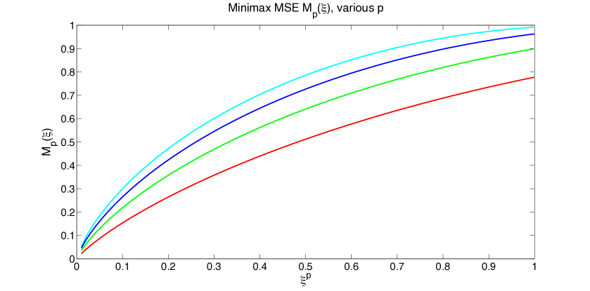
Figure 1: Minimax soft thresholding risk, $M_{p}(\xi)$, various $p$. Vertical axis: worst case MSE over ${\cal F}_{p}(\xi)$. Horizontal axis: $\xi^{p}$. Red, green, blue, aqua curves correspond to $p=0.1,0.25,0.50,1.00$.

The quantity (2.7) can be viewed as the value of a game against Nature, where the statistician chooses the threshold $\tau$, Nature chooses the distribution $\nu$, and the statistician pays Nature an amount equal to the MSE. We use the following notation for the MSE of soft thresholding, given a noise level $\sigma$, a signal distribution $\nu$ and a threshold level $\tau$:

$${\sf mse}(\sigma^{2};\nu,\tau)\equiv{\mathbb{E}}\big{\{}\big{[}\eta(X+\sigma\,Z;\tau\,\sigma)-X\big{]}^{2}\big{\}}\,,$$ (2.8)

where, again, expectation is with respect to $X\sim\nu$ and $Z\sim{\sf N}(0,1)$ independent. Hence the quantity on the right hand side of Eq. (2.7) –the game payoff– is just ${\sf mse}(1;\nu,\tau)$.

Evaluating the supremum in Eq. (2.7) might at first appear hopeless. In reality the computation can be done rather explicitly using the following result.

Lemma 2.1.

The least-favorable distribution $\nu_{p,\xi}$, i.e. the distribution forcing attainment of the worst-case MSE, is supported on 3 points. Explicitly, consider the 3-point mixture distribution

$$\nu_{{\varepsilon},\mu}=(1-{\varepsilon})\delta_{0}+\frac{{\varepsilon}}{2}\delta_{\mu}+\frac{{\varepsilon}}{2}\delta_{-\mu}\,.$$ (2.9)

Then the least-favorable distribution $\nu_{p,\xi}$ is the 3-point mixture $\nu_{{\varepsilon}_{p}(\xi),\mu_{p}(\xi)}$ for specific values ${\varepsilon}_{p}(\xi),\mu_{p}(\xi)$.

In fact it seems the minimax problem in Eq. (2.7) has a saddlepoint, i.e. a pair $(\nu_{p,\xi},\tau_{p}(\xi))\in{\cal P}({\mathbb{R}})\times{\mathbb{R}}_{+}$, such that

$${\sf mse}(1;\nu_{p,\xi},\tau)\geq{\sf mse}(1;\nu_{p,\xi},\tau_{p}(\xi))\geq{\sf mse}(1;\nu,\tau_{p}(\xi))\qquad\forall\tau>0,\;\forall\nu\in{\cal F}_{p}(\xi)\,,$$ (2.10)

but we do not need or prove this fact here. The MSE is readily evaluated for 3-point distribution, yielding

$${\sf mse}(1;\nu_{{\varepsilon},\mu},\tau)=(1-\varepsilon)\big{\{}2(1+\tau^{2})\Phi(-\tau)-2\tau\phi(\tau)\big{\}}$$ (2.11)

$$+\varepsilon\big{\{}\mu^{2}+(1+\tau^{2}-\mu^{2})[\Phi(-\mu-\tau)+\Phi(\mu-\tau)]+(\mu-\tau)\phi(\mu+\tau)-(\mu+\tau)\phi(-\mu+\tau)\big{\}}\,.$$

Here and below, $\phi(z)\equiv e^{-z^{2}/2}/\sqrt{2\pi}$ is the standard Gaussian density and $\Phi(x)\equiv\int_{-\infty}^{x}\phi(z)\,{\rm d}z$ is the Gaussian distribution function. Further, it is easy to check that the MSE is maximized when the $\ell_{p}$ constraint is saturated, i.e. for

$${\varepsilon}\mu^{p}=\xi^{p}\,.$$ (2.12)

Therefore one is left with the task of maximizing the right-hand side of Eq. (2.11) with respect to $\varepsilon$ (for $\mu=\xi\varepsilon^{-1/p}$) and minimizing it with respect to $\tau$. This can be done quite easily numerically for any given $\xi>0$, yielding the values of $\tau_{p}(\xi)$, $\mu_{p}(\xi)$ and ${\varepsilon}_{p}(\xi)$ plotted in Fig. 2. The minimax property is illustrated in Fig. 3.

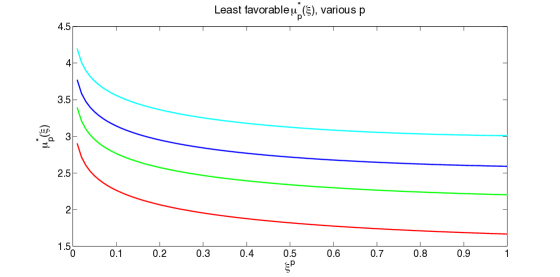
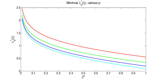
Figure 2: Least-favorable $\mu$ (upper frame) and corresponding minimax threshold $\tau$ (lower frame). Horizontal axes: $\xi^{p}$. Red, green, blue, aqua curves correspond to $p=0.1,0.25,0.50,1.00$.

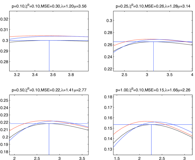
Figure 3: Saddlepoint property of Minimax $\tau_{p}(\xi)$, $\xi^{p}=1/10$, various $p$. Vertical Axis: MSE at $F_{{\varepsilon},\mu}$. Horizontal Axis $\mu$. Vertical Blue line: least-favorable $\mu$, $\mu_{p}(\xi)$. Horizontal Blue Line: Minimax MSE $M_{p}(\xi)$. At each value of $\mu$, Black curve displays corresponding MSE of soft thresholding with threshold at the minimax threshold value $\tau_{p}(\xi)$ , under the distribution $F_{{\varepsilon},\mu}$ with ${\varepsilon}\mu^{p}=\xi^{p}$. The other two curves are for $\tau$ 10 percent higher and 10 percent lower than the minimax value. In each case, the black curve (associated with minimax $\tau$), stays below the horizontal line, while the red and blue curves cross above it, illustrating the saddlepoint relation.

Important below will be the inverse function

$$M_{p}^{-1}(m)=\inf\big{\{}\,\xi\in[0,\infty)\,:\;M_{p}(\xi)\geq m\,\big{\}},$$ (2.13)

defined for $m\in(0,1)$, and depicted in Figure 4. The well-definedness of this function follows from the next Lemma.

Lemma 2.2.

The function $\xi\mapsto M_{p}(\xi)$ is continuous and strictly increasing for $\xi\in(0,\infty)$, with $\lim_{\xi\to 0}M_{p}(\xi)=0$, and $\lim_{\xi\to\infty}M_{p}(\xi)=1$.

Proof.

Let ${\sf mse}_{0}(\mu,\tau)\equiv{\mathbb{E}}\{[\eta(\mu+Z;\tau)-\mu]^{2}\}$ for $Z\sim{\sf N}(0,1)$, so that ${\sf mse}(1;\tau,\nu)=\int{\sf mse}_{0}(\mu,\tau)\,\nu({\rm d}\mu)$. Since ${\sf mse}_{0}(\mu,\tau)={\sf mse}_{0}(-\mu,\tau)$ in this formula we can assume without loss of generality that $\nu(\,\cdot\,)$ is supported on ${\mathbb{R}}_{+}$.

To show strict monotonicity, fix $\xi\leq\xi^{\prime}$, let $\tau^{\prime}=\tau_{p}(\xi^{\prime})$ be the minimax threshold for ${\cal F}_{p}(\xi^{\prime})$, and let $\nu_{\xi}=\nu_{p,\xi}$ be the least favorable prior for ${\cal F}_{p}(\xi)$. Let $\nu^{\prime}=S_{\xi^{\prime}/\xi}\nu_{\xi}$ be the measure in ${\cal F}_{p}(\xi^{\prime})$ obtained by scaling $\nu_{\xi}$ up by a factor $\xi^{\prime}/\xi$ (explicitly, for a measurable set $C$, $\nu^{\prime}(C)=\nu_{\xi}((\xi^{\prime}/\xi)C)$). Since $\nu_{\xi}\neq\delta_{0}$, strict monotonicity of $\mu\rightarrow{\sf mse}_{0}(\mu,\tau)$ (e.g. [DJ94, eq. A2.8]) shows that ${\sf mse}(1;\tau^{\prime},\nu_{\xi})<{\sf mse}(1;\tau^{\prime},\nu^{\prime})$. Consequently

$$M_{p}(\xi)\leq{\sf mse}(1;\tau^{\prime},\nu_{\xi})<{\sf mse}(1;\tau^{\prime},\nu^{\prime})\leq\sup_{\nu\in{\cal F}_{p}(\xi^{\prime})}{\sf mse}(1;\tau^{\prime},\nu)=M_{p}(\xi^{\prime}).$$

We verify that $t\rightarrow M_{p}(t^{1/p})$ is concave in $t$: combined with strict monotonicity, we can then conclude that $M_{p}(\xi)$ is continuous. Indeed, the map $\nu\rightarrow{\sf mse}(1;\tau,\nu)$ is linear in $\nu$ and so ${\sf mse}_{*}(\nu)=\inf_{\tau}{\sf mse}(1;\tau,\nu)$ is concave in $\nu$. Hence $M_{p}(t^{1/p})=\sup\{{\sf mse}_{*}(\nu)~{}:~{}\nu(|X|^{p})\leq t\}$ is also concave.

That $\lim_{\xi\rightarrow 0}M_{p}(\xi)=0$ is shown in [DJ94], compare Lemma 2.3 below. For large $\xi$, observe that

$$1\geq M_{p}(\xi)\geq\mathcal{M}_{p}(\xi)\equiv\inf_{\eta}\sup_{{\cal F}_{p}(\xi)}{\mathbb{E}}\{[\eta(X+Z)-X]^{2}\}\,,$$

the minimax risk over all estimators $\eta$. Further $\mathcal{M}_{p}(\xi)\geq\mathcal{M}_{\infty}(\xi)$, the minimax risk for estimation subject to the bounded mean constraint $|\mu|\leq\xi$. That $\mathcal{M}_{\infty}(\xi)\rightarrow 1$ is shown, for example, in [DLM90, Eq. (2.6)]. ∎

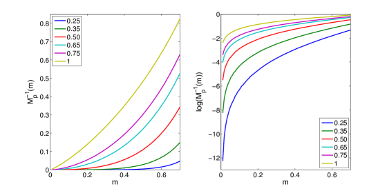
Figure 4: Inverse function $M_{p}^{-1}(m)$. Horizontal axis: $m$, desired minimax mean square error $m$. Vertical axis: left-hand plot: $\xi=M_{p}^{-1}(m)$, the radius of ball that attains it. right-hand plot: $\log(\xi)$. Colored curves correspond to various choices of $p$.

Of particular interest is the case of extremely sparse signals, which corresponds to the limit of small $\xi$. This regime was studied in detail in [DJ94] whose results we summarize below.

Lemma 2.3 ([DJ94]).

As $\xi\to 0$ the minimax pair $(\nu_{{\varepsilon}_{p}(\xi),\mu_{p}(\xi)},\tau_{p}(\xi))$ in Eq. (2.7) obeys

$$\tau_{p}(\xi) = \sqrt{2\log(1/\xi^{p})}\cdot\{1+o(1)\}\,,$$

$$\mu_{p}(\xi) = \sqrt{2\log(1/\xi^{p})}\,\cdot\{1+o(1)\}\,,$$

$${\varepsilon}_{p}(\xi) = \left(\frac{\xi^{2}}{2\log(1/\xi^{p})}\right)^{p/2}\cdot\{1+o(1)\}\,.$$

Further, the minimax mean square error is given, in the same limit, by

$$M_{p}(\xi)=(2\log(1/\xi^{p}))^{1-p/2}\xi^{p}\cdot\{1+o(1)\}\,.$$ (2.14)

The asymptotics for $M_{p}(\xi)$ in the last lemma imply the following behavior of the inverse function as $m\to 0$:

$$M_{p}^{-1}(m)=\big{(}2\log(1/m)\Big{)}^{1/2-1/p}m^{1/p}\cdot\{1+o(1)\}\,.$$ (2.15)

3 The asymptotic LASSO risk

In this section we discuss the high-dimensional limit of the LASSO mean square error for a given sequence of instances ${\sf S}=(I_{n,N})$. Our treatment is mainly a summary of results proved in [BM10] and [DMM10], adapted to the current context.

3.1 Convergent Sequences, and their AMSE

We introduced the notion of sequence of instances as a very general, almost structure-free notion; but certain special sequences play a distinguished role.

Definition 3.1.

Convergent sequence of problem instances. The sequence of problem instances ${\sf S}=\{(x_{0}^{(N)},z^{(n)},A^{(n,N)})\}_{n,N}$ is said to be a convergent sequence if $n/N\to\delta\in(0,\infty)$, and in addition the following conditions hold:

• Convergence of object marginals. The empirical distribution of the entries of $x_{0}^{(N)}$ converges weakly to a probability measure $\nu$ on ${\mathbb{R}}$ with bounded second moment. Further $N^{-1}\|x_{0}^{(N)}\|_{2}^{2}\to{\mathbb{E}}_{\nu}X^{2}$.

• Convergence of noise marginals. The empirical distribution of the entries of $z^{(n)}$ converges weakly to a probability measure $\omega$ on ${\mathbb{R}}$ with bounded second moment. Further $n^{-1}\|z_{i}^{(n)}\|_{2}^{2}\to{\mathbb{E}}_{\omega}Z^{2}\equiv\sigma^{2}$.

• Normalization of Matrix Columns. If $\{e_{i}\}_{1\leq i\leq N}$, $e_{i}\in{\mathbb{R}}^{N}$ denotes the standard basis, then $\max_{i\in[N]}\|A^{(n,N)}e_{i}\|_{2}$, $\min_{i\in[N]}\|A^{(n,N)}e_{i}\|_{2}\to 1$, as $N\to\infty$ where $[N]\equiv\{1,2,\ldots,N\}$.

We shall say that ${\sf S}$ is a convergent sequence of problem instances, and will write ${\sf S}\in CS(\delta,\nu,\omega,\sigma)$ to make explicit the limit objects.

Next we need to introduce or recall some notations. The mean square error for scalar soft thresholding was already introduced in the previous Section, cf. Eq. (2.8), and denoted by ${\sf mse}(\sigma^{2};\nu,\tau)$. The second is the following state evolution map

$$\Psi(m;\delta,\sigma,\nu,\tau)\equiv{\sf mse}\Big{(}\sigma^{2}+\frac{1}{\delta}m;\nu,\tau\Big{)}\,,$$ (3.1)

This is the mean square error for soft thresholding, when the noise variance is $\sigma^{2}+m/\delta$. The addition of the last term reflects the increase of ‘effective noise’ in compressed sensing as compared to simple denoising, due to the undersampling. In order to have a shorthand for the latter, we define noise plus interference to be

$${\sf npi}(m;\delta,\sigma)=\sigma^{2}+\frac{m}{\delta}\,.$$ (3.2)

Whenever the arguments $\delta,\sigma,\nu,\tau$ will be clear from the context in the above functions, we will drop them and write, with an abuse of notation $\Psi(m)$ and ${\sf npi}(m)$.

Finally, we need to introduce the following calibration relation. Given $\tau\in{\mathbb{R}}_{+}$, let $m_{*}(\tau)$ to be the largest positive solution of the fixed point equation

$$m=\Psi(m;\delta,\sigma,\nu,\tau)$$ (3.3)

(of course $m_{*}$ depends on $\delta,\sigma,\nu$ as well but we’ll drop this dependence unless necessary). Such a solution is finite for all $\tau>\tau_{0}$ for some $\tau_{0}=\tau_{0}(\delta)$. The corresponding LASSO parameter is then given by

$$\lambda(\tau)\equiv\tau\sqrt{{\sf npi}_{*}}\left[1-\frac{1}{\delta}{\mathbb{P}}\big{\{}|X+\sqrt{{\sf npi}_{*}}Z|\geq\tau\sqrt{{\sf npi}_{*}}\big{\}}\right]\,.$$ (3.4)

with ${\sf npi}_{*}={\sf npi}(m_{*}(\tau))$. As shown in [BM10], $\tau\mapsto\lambda(\tau)$ establishes a bijection between $\lambda\in(0,\infty)$ and $\tau\in(\tau_{1},\infty)$ for some $\tau_{1}=\tau_{1}(\delta)>\tau_{0}(\delta)$.

The basic high-dimensional limit result can be stated as follows.

Theorem 3.1.

Let ${\sf S}=\{I_{n,N}\}=\{(x_{0}^{(N)},z^{(n)},A^{(n,N)})\}_{n,N}$ be a convergent sequence of problem instances, ${\sf S}\in CS(\delta,\sigma,\nu,\omega)$, and assume also that the matrices $A^{(n,N)}$ are sampled from $\mbox{\sc Gauss}(n,N)$. Denote by $\hat{x}_{\lambda}^{(N)}$ the LASSO  estimator for instance $I_{n,N}$, $\lambda\geq 0$ and let $\psi:{\mathbb{R}}\times{\mathbb{R}}\to{\mathbb{R}}$ be a locally-Lipschitz function with $|\psi(x_{1},x_{2})|\leq C(1+x_{1}^{2}+x_{2}^{2})$ for all $x_{1},x_{2}\in{\mathbb{R}}$.

Then, almost surely

$$\lim_{N\to\infty}\frac{1}{N}\sum_{i=1}^{N}\psi\big{(}\widehat{x}_{\lambda,i},x_{0,i}\big{)}={\mathbb{E}}\Big{\{}\psi\big{(}\eta(X+\sqrt{{\sf npi}_{*}}\,Z;\tau_{*}\sqrt{{\sf npi}_{*}}),X\big{)}\Big{\}}\,,$$ (3.5)

where ${\sf npi}_{*}\equiv{\sf npi}(m_{*})$, $Z\sim{\sf N}(0,1)$ is independent of $X\sim\nu$, $\tau_{*}=\tau_{*}(\lambda)$ is given by the calibration relation described above, and $m_{*}$ is the largest positive solution of the fixed point equation $m=\Psi(m,\delta,\sigma,\nu,\tau_{*})$.

3.2 Discussion and further properties

In the next pages we will repeatedly use the shorthand ${\rm HFP}(\Psi)$ to denote the largest positive solution of the fixed point equation $m=\Psi(m;\delta,\sigma,\nu,\tau)$, where we may suppress the secondary parameters $(\delta,\sigma,\nu,\tau)$ and simply write $\Psi(m)$. Formally

$${\rm HFP}(\Psi)\equiv\sup\{m\geq 0\,:\Psi(m)\geq m\}.$$ (3.6)

In order to emphasize the role of parameters $\delta,\sigma,\nu,\tau$, we may also write
${\rm HFP}(\Psi(\,\cdot\,;\delta,\sigma,\nu,\tau))$. We recall some basic properties of the mapping $\Psi$.

Lemma 3.1 ([DMM09, DMM10]).

For fixed $\delta,\sigma,\nu,\tau$, the mapping $m\mapsto\Psi(m)$ defined on $[0,\infty)$ is continuous, strictly increasing and concave. Further $\Psi(0)\geq 0$ with $\Psi(0)=0$ if and only if $\sigma=0$. Finally, there exists $\tau_{0}=\tau_{0}(\delta)$ such that $\lim_{m\to\infty}\Psi^{\prime}(m)<1$ if and only if $\tau>\tau_{0}$.

By specializing Theorem 3.1 to the case $\psi(x_{1},x_{2})=(x_{1}-x_{2})^{2}$ and using the fixed point condition $m_{*}=\Psi(m_{*};\delta,\sigma,\nu,\tau_{*})$ we obtain immediately the following.

Corollary 3.1.

Let ${\sf S}\in CS(\delta,\sigma,\nu,\omega)$ be a convergent sequence of problem instances, and further assume that $A^{(n,N)}\sim\mbox{\sc Gauss}(n,N)$. Denote by $\hat{x}_{\lambda}^{(N)}$ the LASSO  estimator for problem instance $I_{n,N}$, with $\lambda\geq 0$ . Then, almost surely

$$\lim_{N\to\infty}\frac{1}{N}\|\widehat{x}_{\lambda}-x_{0}\|_{2}^{2}=m_{*}\,,$$ (3.7)

where $m_{*}={\rm HFP}(\Psi(\,\cdot\,;\delta,\sigma,\nu,\tau_{*}))$, and $\tau_{*}=\tau_{*}(\lambda)$ is fixed by the calibration relation (3.4).

3.3 AMSE over General Sequences

Corollary 3.1 determines the asymptotic mean square error for convergent sequences ${\sf S}\in CS(\delta,\sigma,\nu)$. The resulting expression depends on $\delta,\sigma,\nu$, and is denoted ${\rm AMSE}_{SE}(\lambda;\delta,\sigma,\nu)$. We have

$${\rm AMSE}_{SE}(\lambda;\delta,\sigma,\nu)={\rm HFP}(\Psi(\,\cdot\,;\delta,\sigma,\nu,\tau_{*})).$$ (3.8)

The introduction considered instead the asymptotic mean square error ${\rm AMSE}(\lambda;{\sf S})$ along general, not necessarily convergent sequences of problem instances in the standard $\ell_{p}$ problem suite ${\sf S}\in{\cal S}_{p}(\delta,\xi,\sigma)$, cf. Eq. (1.4). Given a sequence ${\sf S}\in{\cal S}_{p}(\delta,\xi,\sigma)$, we let

$${\rm AMSE}(\lambda;{\sf S})=\lim\sup_{N\to\infty}\frac{1}{N}{\mathbb{E}}\big{\{}\|\widehat{x}_{\lambda}^{(N)}-x_{0}^{(N)}\|^{2}\big{\}}\,.$$ (3.9)

Below we will often omit the subscript ${\sc SE}$ on $AMSE_{SE}$, thereby using the same notation for the state evolution quantity (3.8) and the sequence quantity (3.9). This abuse is justified by the following key fact. The asymptotic mean square error along any sequence of instances can be represented by the formula ${\rm AMSE}_{SE}(\lambda;\delta,\nu,\sigma)$, for a suitable $\nu$ – provided the sensing matrices $A^{(n,N)}$ have i.i.d. Gaussian entries. Before stating this result formally, we recall that the definition of sparsity class ${\cal F}_{p}(\xi)$ was given in Eq. (2.6).

Proposition 3.1.

Let ${\sf S}$ be any (not necessarily convergent) sequence of problem instances in ${\cal S}_{p}(\delta,\xi,\sigma)$. Then there exists a probability distribution $\nu\in{\cal F}_{p}(\xi)$ such that

$${\rm AMSE}(\lambda;{\sf S})={\rm AMSE}_{SE}(\lambda;\delta,\nu,\sigma),$$ (3.10)

and both sides are given by the fixed point of the one-dimensional map $\Psi$, namely
${\rm HFP}(\Psi(\,\cdot\,;\delta,\sigma,\nu,\tau_{*}))$. Further, for each ${\varepsilon}>0$,

$$\lim\sup_{N\to\infty}{\mathbb{P}}\Big{\{}\frac{1}{N}\|\widehat{x}_{\lambda}^{(N)}-x_{0}^{(N)}\|_{2}^{2}\geq{\rm AMSE}_{SE}(\lambda;\delta,\nu,\sigma)+{\varepsilon}\Big{\}}=0\,.$$ (3.11)

Conversely, for any $\nu\in{\cal F}_{p}(\xi)$, there exists a sequence of instances ${\sf S}\in{\cal S}_{p}(\delta,\xi,\sigma)$, such that ${\rm AMSE}(\lambda;{\sf S})={\rm AMSE}(\lambda;\delta,\nu,\sigma)$ along that sequence.

Proof.

Given the sequence of problem instances, ${\sf S}=\{x_{0}^{(N)},z^{(n)},A^{(n,N)}\}_{n,N}$, extract a subsequence along which the expected mean square error has a limit equal to the $\lim\sup$ in Eq. (1.4). We will then extract a further subsequence that is a convergent subsequence of problem instances, in the sense of Definition 3.1, hence proving the direct part of our claim, by virtue of Corollary 3.1. (Convergence of the expectation of $\|\widehat{x}_{\lambda}^{(N)}-x_{0}^{(N)}\|^{2}/N$ follows from almost sure convergence together with the fact that $\|x_{0}^{(N)}\|^{2}/N$ is uniformly bounded by assumption and $\|\widehat{x}_{\lambda}^{(N)}\|^{2}/N$ is uniformly bounded by Lemma 3.3 in [BM10].)

Let $\nu_{x_{0},N}$ be the empirical distribution of $x_{0}^{(N)}$ as in (2.5). Since ${\sf S}\in{\cal S}_{p}(\delta,\xi,\sigma)$, we have $\nu_{x_{0},N}(|X|^{p})\leq\xi^{p}$ hence the family $\{\nu_{x_{0},N}\}$ is tight, and along a further subsequence the empirical distributions of $x_{0}^{(N)}$ converge weakly, to a limit $\nu$, say. Again by ${\sf S}\in{\cal S}_{p}(\delta,\xi,\sigma)$, the empirical distributions of $z^{(n)}$ are tight (assumption ${\bf z}\in{\cal Z}^{2}(\sigma)$ entails $\|z^{(n)}\|^{2}/n\to\sigma^{2}$); we extract yet another subsequence along which they converge, to $\omega$, say.

We are left with a subsequence we shall label $\{(n_{k},N_{k})\}_{k\geq 1}$. We wish to prove for this sequence (a)-(c) of Definition 3.1. Property (c) in Definition 3.1, the convergence of column norms, is well known to hold for random matrices with iid Gaussian entries (and easy to show). We are left to show (a) and (b), i.e. that $\nu_{x_{0},N_{k}}(X^{2})\to\nu(X^{2})$ and $\nu_{z,n_{k}}(X^{2})\to\omega(X^{2})$ along this sequence. Convergence of the second moments follows since

$$\lim_{k\to\infty}\nu_{x_{0},N_{k}}(X^{2}) =\lim_{k\to\infty}\nu_{x_{0},N_{k}}(X^{2}{\mathbb{I}}_{\{|X|\leq M\}})+\lim_{k\to\infty}\nu_{x_{0},N_{k}}(X^{2}{\mathbb{I}}_{\{|X|>M\}})$$

$$=\nu(X^{2}{\mathbb{I}}_{\{|X|\leq M\}})+{\sf err}_{M}$$

where we used the dominated convergence theore, where, by the uniform integrability property of sequences ${\bf x}$ in ${\cal X}_{p}(\xi)$, ${\sf err}_{M}\leq\epsilon_{M}\downarrow 0$ as $M\to\infty$.

The limit in probability (3.11) follows by very similar arguments and we omit it here.

The converse is proved by taking $x_{0}^{(N)}$ to be a vector with iid components $x_{0}^{(N)}\sim\nu$. The empirical distributions $\nu_{N}$ then converge almost surely to $\nu$ by the Glivenko-Cantelli theorem. Convergence of second moments follows from the strong law of large numbers. ∎

3.4 Intuition and relation to AMP algorithm

Theorem 3.1 implies that, in the high-dimensional limit, vector estimation through the LASSO can be effectively understood in terms of $N$ uncoupled scalar estimation problems, provided the noise is augmented by an undersampling-dependent increment. A natural question is whether one can construct, starting from the vector of measurements $y=(y_{1},\dots,y_{n})$ (which are intrinsicaly ‘joint’ measurements of $x_{1},\dots,x_{N}$), a collection of $N$ uncoupled measurements of $x_{1},\dots,x_{N}$.

A deeper intuition about this question and Theorem 3.1 can be developed by considering the approximate message passing (AMP) algorithm first introduced in [DMM09]. At one given problem instance (i.e. frozen choice of $(n,N)$) we omit the superscript $(N)$. The algorithm produces a sequence of estimates $\{\widehat{x}^{0},\widehat{x}^{1},\widehat{x}^{2}\,\dots\}$ in ${\mathbb{R}}^{N}$, by letting $\widehat{x}^{0}=0$ and, for each $t\geq 0$

$$z^{t} = y-A\widehat{x}^{t}+\frac{\|\widehat{x}^{t}\|_{0}}{n}\,z^{t-1}$$ (3.12)

$$\widehat{x}^{t+1} = \eta(\widehat{x}^{t}+A^{T}z^{t};\theta_{t})\,,$$ (3.13)

where $\|\widehat{x}^{t}\|_{0}$ is the size of the support of $\widehat{x}^{t}$. Here $\{z^{t}\}_{t\geq 0}\subseteq{\mathbb{R}}^{n}$ is a sequence of residuals and $\theta_{t}$ a sequence of thresholds.

As shown in [BM11], the vector $\widehat{x}^{t}+A^{T}z^{t}$ is distributed asymptotically (large $t$) as $x_{0}+w^{t}$ with $w^{t}\in{\mathbb{R}}^{N}$ a vector with i.i.d. components $w_{i}^{t}\sim{\sf N}(0,\sigma_{t}^{2})$ independent of $x_{0}$. (Here the convergence is to be understood in the sense of finite-dimensional marginals.) In other words, the vector $\widehat{x}^{t}+A^{T}z^{t}$ produced by the AMP algorithm is effectively a vector of i.i.d. uncoupled observations of the signal $x_{0}$.

The second key point is that the AMP algorithm is tightly related to the LASSO. First of all, fixed points of AMP (for a fixed value of the threshold $\theta_{t}=\theta_{*}$) are minimizers of the LASSO cost function and viceversa, provided the $\theta_{*}$ is calibrated with the regularization parameter $\lambda$ according to the following relation

$$\lambda=\theta_{*}\cdot\Big{(}1-\frac{\|\widehat{x}_{\lambda}\|_{0}}{n}\Big{)},$$ (3.14)

with $\widehat{x}_{\lambda}$ the LASSO minimizer or –equivalently– the AMP fixed point. Finally, [BM10] proved that (for Gaussian sensing matrices $A$), the AMP estimates do converge to the LASSO minimizer provided the sequence of thresholds is chosen according to the policy

$$\theta_{t}=\tau\,\sigma_{t}\,,$$ (3.15)

for a suitable $\alpha>0$ depending on $\lambda$ [BM10, DMM10]. Finally, the effective noise-plus-interference level $\sigma_{t}$ can be estimated in several ways, a simple one being $\widehat{\sigma}_{t}^{2}=\|z_{t}\|^{2}/n$.

4 Minimax MSE over $\ell_{p}$ Balls, Noiseless Case

In this section we state results for the noiseless case, $y=Ax_{0}$, where $A$ is $n\times N$ and $x_{0}$ obeys an $\ell_{p}$ constraint. As mentioned in the introduction, our results hold in the asymptotic regime where $n/N\rightarrow\delta\in(0,1)$.

4.1 Main Result

Let ${\sf S}\equiv\{(x_{0}^{(N)},z^{(n)},A^{(n,N)})\}_{n,N}$ be a sequence of noiseless problem instances ($z^{(n)}=0$: no noise is added to the measurements) with Gaussian sensing matrices $A^{(n,N)}\sim\mbox{\sc Gauss}(n,N)$. Define the minimax LASSO mean square error as

$$M_{p}^{*}(\delta,\xi)\equiv\sup_{{\sf S}\in{\cal S}_{p}(\delta,\xi,0)}\inf_{\lambda\in{\mathbb{R}}_{+}}{\rm AMSE}(\lambda;{\sf S})\,.$$ (4.1)

Theorem 4.1.

Fix $\delta\in(0,1)$, $\xi>0$. The minimax AMSE obeys:

$$M_{p}^{*}(\delta,\xi)=\frac{\delta\xi^{2}}{M_{p}^{-1}(\delta)^{2}}.$$ (4.2)

Further we have:

Minimax Threshold. The minimax threshold $\lambda^{*}(\delta,\xi)$ is given by the calibration relation (3.4) with $\tau=\tau^{*}(\delta,\xi)$ determined as follows (notice in particular that this is independent of $\xi$):

$$\tau^{*}(\delta,\xi)=\tau_{p}(M_{p}^{-1}(\delta))\,.$$ (4.3)

Least Favorable $\nu$. The least-favorable distribution is a 3-point distribution $\nu^{*}=\nu_{p,\delta,\xi}^{*}=\nu_{{\varepsilon}^{*},\mu^{*}}$ (cf. Eq. (2.9)) with

$$\mu^{*}(\delta,\xi)=\frac{\xi}{M_{p}^{-1}(\delta)}\,\mu_{p}(M^{-1}_{p}(\delta))\,,\;\;\;\;\;{\varepsilon}^{*}(\delta,\xi)=\frac{\xi^{p}}{(\mu^{*})^{p}}\,.$$ (4.4)

Saddlepoint. The above quantities obey a saddlepoint relation. Put for short ${\rm AMSE}(\lambda;\nu)$ in place of ${\rm AMSE}(\lambda;\delta,\nu,0)$, The minimax AMSE obeys

$$M_{p}(\delta;\xi)={\rm AMSE}(\lambda^{*};\nu^{*})$$

and

$${\rm AMSE}(\lambda^{*};\nu^{*}) \leq {\rm AMSE}(\lambda;\nu^{*})\,,\qquad\forall\lambda>0$$ (4.5)

$$\geq {\rm AMSE}(\lambda^{*};\nu)\,,\qquad\forall\nu\in{\cal F}_{p}(\xi).$$ (4.6)

4.2 Interpretation

Figure 5 presents the function $M_{p}^{*}(\delta,\xi=1)$ on a logarithmic scale. As the reader can see, there is a substantial increase in the minimax risk as $\delta\rightarrow 0$, which agrees with our intuitive picture that the reconstruction becomes less accurate for small $\delta$ (high undersampling).

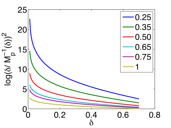
Figure 5: Minimax MSE $M_{p}^{*}(\delta,1)$. We assume here $\xi=1$; curves show $\log$ MSE as a function of $\delta$. Consistent with $\delta\rightarrow 0$ asymptotic theory, the curves are nearly scaled copies of each other.

The asymptotic properties of $M_{p}^{*}(\delta,1)$ in the high undersampling regime ($\delta\to 0$) can be derived using Lemma 2.3. From Eq. (2.15) we have

$$M_{p}^{*}(\delta,1)=\delta^{1-2/p}(2\log(\delta^{-1}))^{2/p-1}\big{\{}1+o_{\delta}(1)\big{\}},\qquad\delta\rightarrow 0.$$

Hence, when plotting $\log M_{p}^{*}(\delta,1)$, as we do here, we should see graphs of the form

$$\log M_{p}^{*}(\delta,1)=(1-2/p)\cdot\left[\log(\delta^{-1})-\log(\log(\delta^{-1}))-\log(2)\right]+o_{\delta}(1),\qquad\delta\rightarrow 0.$$

In particular the curves should look ‘all the same’ at small $\delta$, except for scaling; this is qualitatively consistent with Fig 5, even at larger $\delta$.

Another useful prediction can be obtained by working out the asymptotics of the minimax threshold $\lambda^{*}(\delta,\xi)$. Using Eq. (4.3) as well as the calibration relation (3.4), we get, as $\delta\to 0$,

$$\lambda^{*}(\delta,\xi)=\xi\,\cdot\Big{(}\frac{2\log(1/\delta)}{\delta}\Big{)}^{1/p}\,\big{\{}1+o_{\delta}(1)\big{\}}\,.$$ (4.7)

4.3 Proof of Theorem 4.1

We will focus on proving Eq. (4.2), since the other points follow straightforwardly. By Proposition 3.1, we have the equivalent characterization

$$M_{p}^{*}(\delta,\xi)=\sup_{\nu\in{\cal F}_{p}(\xi)}\inf_{\lambda\in{\mathbb{R}}_{+}}{\rm AMSE}(\lambda;\delta,\nu,\sigma=0)\,.$$ (4.8)

Further, by Corollary 3.1, we can use the mean square error expression given there, and because of the monotone nature of the calibration relation, we can minimize over the threshold $\tau$ instead of $\lambda$. We get therefore

$$M_{p}^{*}(\delta,\xi)=\sup_{\nu\in{\cal F}_{p}(\xi)}\inf_{\tau\in{\mathbb{R}}_{+}}{\rm AMSE}_{\mbox{\tiny\rm SE}}(\tau;\delta,\nu,0)\,,$$ (4.9)

where

$${\rm AMSE}_{\mbox{\tiny\rm SE}}(\tau;\delta,\nu,0) =m\,,$$

$$m ={\sf mse}\big{(}m/\delta;\nu,\tau)\,.$$ (4.10)

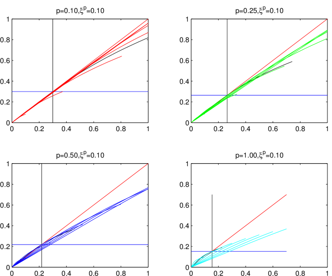
Figure 6: Illustration of the minimax fixed point property. Horizontal input MSE $m$. Vertical: output MSE $\Psi(m)$ for the state evolution map defined as per Eq. (3.1). Red diagonal: $\Psi(m)=m$. Black vertical Line: minimax HFP $M_{p}(\xi)$. Blue horizontal line: minimax MSE $M_{p}(m)$. Black curve: MSE map at minimax threshold value and least-favorable distribution. It crosses the diagonal at the minimax fixed point. Colored Curves. MSE maps at minimax threshold value and other three-point distributions. All other fixed points occur below $M_{p}(\xi)$.

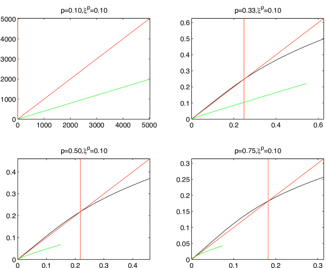
Figure 7: Comparisons of highest fixed point at power law distribution with minimax HFP. Horizontal input MSE $m$. Vertical: output MSE $\Psi(m)$ for the state evolution map defined as per Eq. (3.1). Red diagonal: $\Psi(m)=m$. Red vertical: Minimax MSE. Black curve: MSE map at minimax threshold value and least-favorable distribution. It crosses the diagonal at the minimax fixed point. Green Curve: MSE map with same threshold, taken at power law distribution calibrated to same ${\mathbb{E}}|X|^{p}=\xi^{p}$ constraint.

Recall that ${\cal P}({\mathbb{R}})$ denotes the class of all probability distribution functions on ${\mathbb{R}}$. Define the scaling operator $S_{a}:{\cal P}({\mathbb{R}})\to{\cal P}({\mathbb{R}})$ by $(S_{a}\nu)(B)=\nu(B/a)$ for any Borel set $B$. For the family of operators $\{S_{a}:a>0\}$ we have the group properties

$$S_{a}\cdot S_{b}=S_{a\cdot b},\qquad S_{1}={\bf I},\qquad S_{a}S_{a^{-1}}=S_{1}.$$ (4.11)

In particular by the last property, for any $a>0$, the operator $S_{a}:{\cal P}({\mathbb{R}})\mapsto{\cal P}({\mathbb{R}})$ is one-to-one.

With this notation, we have the scale covariance property of the soft-thresholding mean square error

$${\sf mse}(\sigma^{2};\nu,\tau)=\sigma^{2}\cdot{\sf mse}(1;S_{1/\sigma}\nu,\tau),$$ (4.12)

transforming a general-noise-level problem into a noise-level-one problem. As a consequence of Lemma 3.1, the map $\sigma^{2}\mapsto{\sf mse}(\sigma^{2};\nu,\tau)$ is (for fixed $\nu,\tau$) increasing and concave. Therefore, the map $\sigma^{2}\mapsto{\sf mse}(1;S_{1/\sigma}\nu,\tau)$ is strictly monotone decreasing. Also, the fixed point Eq. (4.10) can be rewritten as

$$\delta={\sf mse}(1;S_{\sqrt{\delta/m}}\nu,\tau)\,,$$ (4.13)

where the solution is unique by strict monotonicity of $m\mapsto{\sf mse}(1;S_{\sqrt{\delta/m}}\nu,\tau)$.

We will prove Eq. (4.2) by obtaining an upper and a lower bound for $M_{p}(\delta,\xi)$. In the following we assume without loss of generality that the infimum in Eq. (4.8) is achieved

$$M_{p}(\delta,\xi)={\rm AMSE}_{\mbox{\tiny\rm SE}}(\tau_{*};\nu_{*},0)\,.$$ (4.14)

Further we will use the minimax conditions for soft thresholding, see Lemma 2.1:

$$\inf_{\tau\in{\mathbb{R}}_{+}}{\sf mse}(1;\nu,\tau) \leq M_{p}(\xi)\,,\;\;\;\;\;\forall\,\nu\in{\cal F}_{p}(\xi)\,,$$ (4.15)

$$\sup_{\nu\in{\cal F}_{p}(\xi)}{\sf mse}(1;\nu,\tau) \geq M_{p}(\xi)\,,\;\;\;\;\;\forall\,\tau\in{\mathbb{R}}_{+}\,.$$ (4.16)

Upper bound on $M_{p}(\delta,\xi)$. Let $m_{*}=M_{p}(\delta,\xi)={\rm AMSE}_{\mbox{\tiny\rm SE}}(\tau_{*};\nu_{*},0)$. By Eq. (4.10) and (4.13) we have

$$\delta={\sf mse}(1;S_{\sqrt{\delta/m_{*}}}\nu_{*},\tau_{*})=\inf_{\tau\in{\mathbb{R}}_{+}}{\sf mse}(1;S_{\sqrt{\delta/m_{*}}}\nu_{*},\tau)\,.$$ (4.17)

The second equality follows because otherwise by there would exist $\tau_{**}$ with ${\sf mse}(1;S_{\sqrt{\delta/m_{*}}}\nu_{*},\tau_{**})$ whence, by the monotonicity of $m\mapsto{\sf mse}(1;S_{\sqrt{\delta/m}}\nu_{*},\tau_{**})$ it would follow that ${\rm AMSE}_{\mbox{\tiny\rm SE}}(\tau_{**};\nu_{*},0)<{\rm AMSE}_{\mbox{\tiny\rm SE}}(\tau_{*};\nu_{*},0)$ which violates the minimax property (4.14).

Next notice that $S_{\sqrt{\delta/m_{*}}}\nu_{*}\in{\cal F}_{p}(\sqrt{\delta/m_{*}}\,\xi)$ whence by Eq. (4.15), we get $\delta\leq M_{p}(\sqrt{\delta/m_{*}}\,\xi)$. By the monotonicity of $\xi\mapsto M_{p}(\xi)$ this yields

$$m_{*}\leq\frac{\delta\,\xi^{2}}{M_{p}^{-1}(\delta)^{2}}\,.$$ (4.18)

Lower bound on $M_{p}(\delta,\xi)$. Again by Eq. (4.10) and (4.13) we have

$$\delta={\sf mse}(1;S_{\sqrt{\delta/m_{*}}}\nu_{*},\tau_{*})=\sup_{\nu\in{\cal F}_{p}(\xi)}{\sf mse}(1;S_{\sqrt{\delta/m_{*}}}\nu,\tau_{*}(\nu))\,,$$ (4.19)

with $\tau_{*}(\nu)$ the optimal threshold for distribution $\nu$ and the second equality following by an argument similar to the one above (i.e. if this weren’t true, there would be a different worst distribution $\nu_{**}$, reaching contradiction). But $\nu\in{\cal F}_{p}(\xi)$ implies $S_{\sqrt{\delta/m_{*}}}\nu\in{\cal F}_{p}(\sqrt{\delta/m_{*}}\,\xi)$, whence

$$\delta=\sup_{\nu\in{\cal F}_{p}(\xi\sqrt{\delta/m_{*}})}{\sf mse}(1;\nu,\tau_{*}(\nu))\geq M_{p}(\sqrt{\delta/m_{*}}\,\xi)\,,$$ (4.20)

where the second inequality follows by Eq. (4.16). The proof is finished by using again the monotonicity of $\xi\mapsto M_{p}(\xi)$. ∎

5 Minimax MSE over $\ell_{p}$ Balls, Noisy Case

In this section we generalize the results of the previous section to the case of noisy measurements with noise variance per coordinate equal to $\sigma^{2}$.

5.1 Main Result

Now let $\sigma>0$ and consider sequences ${\sf S}$ of noisy problem instances from the standard $\ell_{p}$ problem suite ${\sf S}\in{\cal S}_{p}(\delta,\xi,\sigma)$; hence, in addition to the $\ell_{p}$ constraint $\|x_{0}^{(N)}\|_{p}^{p}\leq N\xi^{p}$ and each $A^{(n,N)}\sim\mbox{\sc Gauss}(n,N)$, now the noise vectors $z^{(n)}\in{\mathbb{R}}^{n}$ are non-vanishing and have norms satisfying $\|z^{(n)}\|^{2}/n\to\sigma^{2}>0$.

We define the minimax LASSO asymptotic mean square error as

$$M_{p}^{*}(\delta,\xi,\sigma)\equiv\sup_{{\sf S}\in{\cal S}_{p}(\delta,\xi,\sigma)}\inf_{\lambda\in{\mathbb{R}}_{+}}{\rm AMSE}(\lambda;{\sf S})\,.$$ (5.1)

By simple scaling of the problem we have, for any $\sigma>0$,

$$M_{p}^{*}(\delta,\xi,\sigma)=\sigma^{2}\,M_{p}^{*}(\delta,\xi/\sigma,1)\,,$$ (5.2)

an observation which will be used repeatedly in the following.

Theorem 5.1.

For any $\delta,\xi>0$, let $m^{*}=m^{*}_{p}(\delta,\xi)$ be the unique positive solution of

$$\frac{m^{*}}{1+m^{*}/\delta}=M_{p}\left(\frac{\xi}{(1+m^{*}/\delta)^{1/2}}\right)\,.$$ (5.3)

Then the LASSO minimax mean square error $M_{p}^{*}$is given by:

$$M_{p}^{*}(\delta,\xi,\sigma)=\sigma^{2}\cdot m^{*}(\delta,\xi/\sigma)\,.$$ (5.4)

Further, denoting by $\xi^{*}\equiv(1+m^{*}/\delta)^{-1/2}\xi/\sigma$, we have:

Least Favorable $\nu$. The least-favorable distribution is a $3$-point mixture $\nu^{*}=\nu^{*}_{p,\delta,\xi,\sigma}=\nu_{{\varepsilon}^{*},\mu^{*}}$ (cf. Eq. (2.9)) with

$$\mu^{*}(\delta,\xi,\sigma)=\sigma\cdot(1+m^{*}/\delta)^{1/2}\mu_{p}(\xi^{*}),\;\;\;\;\;{\varepsilon}^{*}(\delta,\xi,\sigma)=\frac{\xi^{p}}{(\mu^{*})^{p}}\,,$$ (5.5)

with $m^{*}=m^{*}(\delta,\xi/\sigma)$ given by the solution of Eq. (5.3)

Minimax Threshold. The minimax threshold $\lambda^{*}(\delta,\xi,\sigma)$ is given by the calibration relation (3.4) with $\tau=\tau^{*}(\delta,\xi,\sigma)$ determined as follows:

$$\tau^{*}(\delta,\xi,\sigma)=\tau_{p}(\xi^{*}).$$ (5.6)

with $\tau_{p}(\,\cdot\,)$ the soft thresholding minimax threshold, $\xi^{*}\equiv(1+m^{*}/\delta)^{-1/2}\xi/\sigma$ and $\nu=\nu^{*}$ is the least favorable distribution given above.

Saddlepoint. The above quantities obey a saddlepoint relation. Put for short ${\rm AMSE}(\lambda;\nu)$ in place of ${\rm AMSE}(\lambda;\delta,\nu,\sigma)$. The minimax AMSE obeys

$$M_{p}(\delta,\xi,\sigma)={\rm AMSE}(\lambda^{*};\nu^{*})\,,$$

and

$${\rm AMSE}(\lambda^{*};\nu^{*}) \leq {\rm AMSE}(\lambda;\nu^{*})\,,\qquad\forall\lambda>0$$ (5.7)

$$\geq {\rm AMSE}(\lambda^{*};\nu)\,,\qquad\forall\nu\in{\cal F}_{p}(\xi).$$ (5.8)

5.2 Interpretation

Figure 8 provides a concrete illustration of Theorem 5.1. For various sparsity levels $\xi$ and undersampling factors $\delta$, the mean square error $M_{p}(\delta,\xi,\sigma)$ can be easily computed. As expected, the result is monotone increasing in $\xi$ and decreasing in $\delta$. For a given target mean square error, such plots allow to determine the required number of linear measurements.

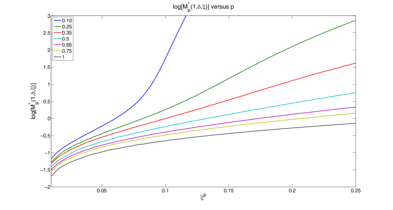
Figure 8: Minimax MSE $M_{p}^{*}(\delta,\xi,1)$, noisy case $\sigma=1$. We assume here $\delta=1/4$; curves show ${\rm MSE}$ as a function of $\xi$.

Equations (5.3) and (5.4) are somewhat more complex that their noiseless counterpart. For this reason, it is instructive to work out the $\sigma\to 0$ limit $M_{p}^{*}(\delta,\xi,\sigma)$. By the basic scaling relation (5.4), this is equivalent to computing the $\xi\to\infty$ limit of $M_{p}^{*}(1,\delta,\xi)=m^{*}(\delta,\xi)$. Considering Eq. (5.3), it is easy to show that, for large $\xi$

$$m^{*}(\delta,\xi)=c_{0}(\delta)\xi^{2}+c_{1}(\delta)+O(\xi^{-2})\equiv c(\delta,\xi)\xi^{2}\,.$$

Substituting in Eq. (5.3)

$$\delta\left(1+\frac{\delta}{c\xi^{2}}\right)^{-1}=M_{p}\left((\delta/c)^{1/2}\left(1+\frac{\delta}{c\xi^{2}}\right)^{-1/2}\right)\,,$$

whence expanding for large $\xi$

$$\delta-\frac{\delta^{2}}{c_{0}\xi^{2}}+O(\xi^{-4})=M_{p}((\delta/c_{0})^{1/2})-\frac{\delta^{1/2}}{2\xi^{2}c_{0}^{3/2}}\,M_{p}^{\prime}((\delta/c_{0})^{1/2})\,(c_{1}+\delta)+O(\xi^{-4})\,.$$

Imposing each order to vanish we get

$$c_{0}(\delta) = \frac{\delta}{M_{p}^{-1}(\delta)}\,,$$ (5.9)

$$c_{1}(\delta) = \frac{2\sqrt{c_{0}\delta}}{M_{p}^{\prime}((\delta/c_{0})^{1/2})}-\delta\,.$$ (5.10)

Our calculations can be summarized as follows.

Corollary 5.1.

Fix a radius parameter $\xi$. As $\sigma^{2}\to 0$, the asymptotic LASSO minimax mean square error behaves as

$$M_{p}^{*}(\delta,\xi,\sigma)=\xi^{2}\,c_{0}(\delta)+\sigma^{2}\,c_{1}(\delta)+O(\sigma^{4}/\xi^{2})\,,$$ (5.11)

with $c_{0}$ and $c_{1}$ determined by Eqs. (5.9) and (5.10). In particular, in the high undersampling regime $\delta\to 0$, we get

$$c_{1}(\delta)=\frac{2}{p}\{1+o_{1}(\delta)\}\,.$$ (5.12)

The derivation of the asymptotic behavior (5.12) is a straightforward calculus exercise, using Lemma 2.3.

The last Corollary shows that the noiseless case, cf. Theorem 4.1 and Eq. (4.2), is recovered as a special case of the noisy case treated in this section. Further leading corrections due to small noise $\sigma^{2}\ll\xi^{2}$ are explicitly described by the coefficient $c_{1}(\delta)$ given in Eq. (5.10).

An alternative asymptotic of interest consists in fixing the noise level $\sigma$, and letting $\xi/\sigma\to 0$. In this regime the solution of Eq. (5.3) yields, using Lemma 2.3,

$$m^{*}(\delta,\xi)=(2\log(1/\xi^{p}))^{1-p/2}\xi^{p}\cdot\{1+o(1)\}\,.$$ (5.13)

Substituting this expression in Theorem 5.1, we obtain the following.

Corollary 5.2.

Fix a noise parameter $\sigma^{2}>0$. As $\xi\to 0$, the asymptotic LASSO minimax mean square error behaves as

$$M_{p}^{*}(\delta,\xi,\sigma)=\sigma^{2-p}\xi^{p}\cdot\big{\{}2\log\big{(}(\sigma/\xi)^{p}\big{)}\big{\}}^{1-p/2}\cdot\{1+o(1)\}\,,$$ (5.14)

Further the minimax threshold value is given, in this limit, by

$$\lambda^{*}=\sigma\cdot\sqrt{2\log\big{(}(\sigma/\xi)^{p}\big{)}}\,\big{\{}1+o(1)\big{\}}\,.$$ (5.15)

5.3 Proof of Theorem 5.1

The argument is structurally similar to the noiseless case. We will focus again on proving the asymptotic expression for minimax error given in Eq. (5.4), since the other points of the theorem follow easily. Using Proposition 3.1 and Corollary 3.1, the asymptotic mean square error can be replaced by the expression given there and the minimization over $\lambda$ can be replaced by a minimization over $\tau$:

$$M_{p}^{*}(\delta,\xi,\sigma)=\sup_{\nu\in{\cal F}_{p}(\xi)}\inf_{\tau\in{\mathbb{R}}_{+}}{\rm AMSE}_{\mbox{\tiny\rm SE}}(\tau;\delta,\nu,\sigma)\,,$$ (5.16)

where

$${\rm AMSE}_{\mbox{\tiny\rm SE}}(\tau;\delta,\nu,\sigma) =m\,,$$

$$m ={\sf mse}\big{(}\sigma^{2}+m/\delta;\nu,\tau)\,.$$ (5.17)

By virtue of the scaling relation (5.2), we can focus on the case $\sigma^{2}=1$. Define, for all $m<\delta$

$${\sf n}(m)\equiv(1+m/\delta)^{-1/2}\,.$$ (5.18)

We then have, applying Eq. (5.17) for the case $\sigma=1$,

$$\frac{m}{1+m/\delta}={\sf mse}\big{(}1;S_{{\sf n}(m)}\nu,\tau)\,.$$ (5.19)

Notice that $m\mapsto m/(1+m/\delta)$ is monotone increasing, and $m\mapsto{\sf mse}\big{(}1;S_{{\sf n}(m)}\nu,\tau)$ is monotone decreasing (because $a^{2}\mapsto{\sf mse}\big{(}1;S_{1/a}\nu,\tau)$ is decreasing as mentioned in the previous section). Hence this equation has a unique non-negative solution provided $\delta>{\sf mse}\big{(}1;\delta,\tau)$, which happens for all $\tau>\tau_{0}(\delta)$.

Assume without loss of generality that the minimax risk is achieved by the pair $(\tau_{*},\nu_{*})$. Then

$$M_{p}^{*}(\delta,\xi,1)={\rm AMSE}_{\mbox{\tiny\rm SE}}(\tau_{*};\delta,\nu_{*},1)=m_{*}\,.$$ (5.20)

Then $m_{*}$ satisfies Eq. (5.19) with $\tau=\tau_{*}$ and $\nu=\nu_{*}$.

Upper bound on $M_{p}(\delta,\xi,1)$. By the last remarks, we have

$$\frac{m_{*}}{1+m_{*}/\delta}={\sf mse}\big{(}1;S_{{\sf n}(m_{*})}\nu_{*},\tau_{*})=\inf_{\tau\in{\mathbb{R}}_{+}}{\sf mse}\big{(}1;S_{{\sf n}(m_{*})}\nu_{*},\tau)\,.$$ (5.21)

The second equality follows from Eq. (5.20). Indeed if the equality did not hold, we could find $\tau_{**}\in{\mathbb{R}}_{+}$ such that ${\sf mse}\big{(}1;S_{{\sf n}(m_{*})}\nu_{*},\tau_{**})<{\sf mse}\big{(}1;S_{{\sf n}(m_{*})}\nu_{*},\tau_{*})$. But by the monotonicity of $m\mapsto m/(1+m/\delta)$ and of $m\mapsto{\sf mse}\big{(}1;S_{{\sf n}(m)}\nu_{*},\tau_{**})$, this would mean that the corresponding fixed point $m_{**}$ is strictly smaller than $m_{*}$. This would contradict the minimax assumption.

Since $S_{{\sf n}(m_{*})}\nu_{*}\in{\cal F}_{p}({\sf n}(m_{*})\xi)$ we can now apply Eq. (4.15), getting

$$\frac{m_{*}}{1+m_{*}/\delta}\leq M_{p}({\sf n}(m_{*})\xi)\,.$$ (5.22)

Again by monotonicity of $m\mapsto m/(1+m/\delta)$ and of $\xi\mapsto M_{p}(\xi)$, this means that $m_{*}$ is upper bounded by the solution of Eq. (5.3).

Lower bound on $M_{p}(1,\delta,\xi)$. Applying again Eq. (5.19) and an analogous argument as above, we have

$$\frac{m_{*}}{1+m_{*}/\delta}=\sup_{\nu\in{\cal F}_{p}(\xi)}{\sf mse}\big{(}1;S_{{\sf n}(m_{*})}\nu,\tau_{*}(S_{{\sf n}(m_{*})}\nu))\,.$$ (5.23)

In the last expression $\tau_{*}(S_{{\sf n}(m_{*})}\nu)$ is the optimal (minimal MSE) threshold for distribution $S_{{\sf n}(m_{*})}\nu$. For $\nu\in{\cal F}_{p}(\xi)$, $S_{{\sf n}(m_{*})}\nu\in{\cal F}_{p}({\sf n}(m_{*})\xi)$. Further the map $S_{{\sf n}(m_{*})}:{\cal F}_{p}(\xi)\to{\cal F}_{p}({\sf n}(m_{*})\xi)$ is bijective. We thus have

$$\frac{m_{*}}{1+m_{*}/\delta}=\sup_{\nu\in{\cal F}_{p}({\sf n}(m_{*})\xi)}{\sf mse}\big{(}1;\nu,\tau_{*}(\nu))\,.$$ (5.24)

By Eq. (4.16), we thus have

$$\frac{m_{*}}{1+m_{*}/\delta}\leq M_{p}({\sf n}(m_{*})\xi)\,,$$ (5.25)

which implies that $m_{*}$ is upper bounded by the solution of Eq. (5.3). This finishes our proof. ∎

6 Weak $p$-th Moment Constraints

Our results for $\ell_{p}$ constraints have natural counterparts for weak $\ell_{p}$ constraints. We recall a standard definition for the weak-$\ell_{p}$ quasi-norm $\|x\|_{w\ell_{p}}$. For a vector $x\in{\mathbb{R}}^{N}$, let $T_{x}(t)\equiv\{i\in\{1,\dots,N\}\;:\;|x_{i}|\geq t\}$ index the entries of $x$ with amplitude above threshold $t$. Denoting by $|S|$ the cardinality of set $S$, we define

$$\|x\|_{w\ell_{p}}\equiv\max_{t\geq 0}\big{[}\,t|T_{x}(t)|^{1/p}\big{]}\,,\qquad$$ (6.1)

By Markov’s inequality $\|x\|_{w\ell_{p}}\leq\|x\|_{p}$: the weak $\ell_{p}$ quasi-norm is indeed weaker than the $\ell_{p}$ norm (quasi norm, if $p<1$). Weak-$\ell_{p}$ norms arise frequently in applied harmonic analysis, as we discuss below.

As the reader no doubt expects, we can define a weak $\ell_{p}$ analogue to the $\ell_{p}$ case.

Definition 6.1.

• Weak $\ell_{p}$ constraint. A sequence ${\bf x}_{0}=(x_{0}^{(N)})$ belongs to ${\cal X}^{w}_{p}(\xi)$ if $(i)$ $\|x_{0}^{(N)}\|_{w\ell_{p}}^{p}\leq N\xi^{p}$, for all $N$; and $(ii)$ there exists a sequence $B=\{B_{M}\}_{M\geq 0}$ such that $B_{M}\to 0$, and for every $N$, $\sum_{i=1}^{N}(x_{0,i}^{(N)})^{2}{\mathbb{I}}(|x_{0,i}^{(N)}|\geq M)\leq B_{M}N$.

• Standard Weak-$\ell_{p}$ Problem Suite. Let ${\cal S}_{p}^{w}(\delta,\xi,\sigma)$ denote the class of sequences of problem instances $I_{n,N}=(x_{0}^{(N)},z^{(n)},A^{(n,N)})$ built from objects in weak $\ell_{p}$; in detail:
  (i) $n/N\rightarrow\delta$;
  (ii) ${\bf x}_{0}\in{\cal X}_{p}^{w}(\xi)$;
  (iii) ${\bf z}\in{\cal Z}_{2}(\sigma)$, and
  (iv) $A^{(n,N)}\in\mbox{\sc Gauss}(n,N)$.

6.1 Scalar Minimax Thresholding under Weak $p$-th Moment Constraints

The class of probability distributions corresponding to instances in the weak-$\ell_{p}$ problem suite is

$${\cal F}^{w}_{p}(\xi)\equiv\Big{\{}\nu\in{\cal P}({\mathbb{R}})\,:\,\sup_{t\geq 0}t^{p}\cdot\nu(\{|X|\geq t\})\leq\xi^{p}\Big{\}}\,.$$ (6.2)

In particular, given a sequence ${\bf x}_{0}\in{\cal X}^{w}_{p}(\xi)$ , the empirical distribution of each $x_{0}^{(N)}$ is in ${\cal F}^{w}_{p}(\xi)$.

As in section 2, we denote by ${\sf mse}(\sigma^{2};\nu,\tau)$ the mean square error of scalar soft thresholding for a given signal distribution $\nu$.

Definition 6.2.

The minimax mean squared error under the weak $p$-th moment constraint is

$$M_{p}^{w}(\xi)=\inf_{\tau\in{\mathbb{R}}_{+}}\sup_{\nu\in{\cal F}_{p}^{w}(\xi)}{\mathbb{E}}\big{\{}\big{[}\eta(X+Z;\tau)-X\big{]}^{2}\big{\}}\,,$$ (6.3)

where the expectation on the right hand side is taken with respect to $X\sim\nu$ and $Z\sim{\sf N}(0,1)$, $X$ and $Z$ independent.

The collection of probability measures ${\cal F}_{p}^{w}(\xi)$ has a distinguished element – a most dispersed one. In fact define the envelope function

$$H_{p,\xi}(t)=\inf_{\nu\in{\cal F}_{p}^{w}(\xi)}\nu(\{|X|\leq t\})\,;$$ (6.4)

the envelope of achievable dispersion of the probability mass for elements of ${\cal F}_{p}^{w}(\xi)$. This envelope can be computed explicitly, yielding

$$H_{p,\xi}(t)=\left\{\begin{array}[]{ll}0&\mbox{for $t<\xi$,}\\ 1-(\xi/t)^{p}&\mbox{for $t\geq\xi$.}\end{array}\right.$$ (6.7)

Indeed it is clear by definition that $\nu(\{|X|\leq t\})\geq H_{p,\xi}(t)$. Further defining the CDF

$$F_{p,\xi}^{w}(x)=\left\{\begin{array}[]{ll}\frac{1}{2}+\frac{1}{2}H_{p}(|x|)&\mbox{for $x\geq 0$},\\ \frac{1}{2}H_{p}(|x|)&\mbox{for $x<0$}.\end{array}\right.$$ (6.10)

and letting $\nu_{p,\xi}$ be the corresponding measure, we get for any $t\geq 0$, $\nu_{p,\xi}(\{|X|\leq t\})=F_{p,\xi}^{w}(t)-F_{p,\xi}^{w}(-t)=H_{p,\xi}(t)$. We therefore proved the following.

Lemma 6.1.

The most dispersed symmetric probability measure in ${\cal F}_{p}^{w}(\xi)$ is $\nu_{p,\xi}$. This distribution achieves the equality $\nu_{p,\xi}(\{|X|\leq t\})=H_{p,\xi}(t)\leq\nu(\{|X|\leq t\})$ for all $\nu\in{\cal F}_{p}^{w}(\xi)$, and all $t>0$.

It turns out that this most dispersed distribution is also the least favorable distribution for soft thresholding. In order to see this fact, define the function ${\sf mse}_{0}:{\mathbb{R}}\times{\mathbb{R}}_{+}\to{\mathbb{R}}$ by letting

$${\sf mse}_{0}(x;\tau)={\mathbb{E}}\big{\{}[\eta(x+Z;\tau)-x]^{2}\big{\}}\,,$$ (6.11)

whereby expectation is taken with respect to $Z\sim{\sf N}(0,1)$. We then have the following useful calculus lemma (see for instance [DMM09].

Lemma 6.2.

For each $\tau\in[0,\infty)$, the mapping $x\mapsto{\sf mse}_{0}(x;\tau)$ is strictly monotone increasing in $x\in[0,\infty)$.

Now the mean square error of scalar soft thresholding, cf. Eq. (2.8), is given by

$${\sf mse}(1;\nu,\tau)\equiv{\mathbb{E}}{\sf mse}_{0}(|X|;\tau)\,,$$ (6.12)

where expectation is taken with respect to $X\sim\nu$. From the above remarks, we obtain immediately the following characterization of the minimax problem.

Corollary 6.1 (Saddlepoint).

Consider the game against Nature where the statistician chooses the threshold $\tau$, Nature chooses the distribution $\nu\in{\cal F}_{p}^{w}(\xi)$, and the statistician pays Nature an amount equal to the mean square error ${\sf mse}(1;\tau,\nu)$.

This game has a saddlepoint $(\tau_{p}^{w}(\xi),\nu_{p,\xi}^{w})$, i.e. a pair satisfying

$${\sf mse}(1;\tau,\nu_{p,\xi}^{w})\geq{\sf mse}(1;\tau_{p}^{w}(\xi),\nu_{p,\xi}^{w})\geq{\sf mse}(1;\tau_{p}^{w}(\xi),\nu)\qquad\forall\tau>0,\;.$$ (6.13)

for all $\tau\geq 0$, and $\nu\in{\cal F}_{p}^{w}(\xi)$. In particular, the least-favorable probability measure is $\nu_{p,\xi}^{w}=\nu_{p,\xi}$, with distribution $F_{p,\xi}$ given in closed form by Eq. (6.10), and we have the following formula for the soft thresholding minimax risk:

$$M_{p}^{w}(\xi)=\inf_{\tau\geq 0}{\sf mse}(1;\tau,\nu_{p,\xi})\,.$$ (6.14)

Ordinarily, identifying a saddlepoint requires search over two variables, namely the threshold $\tau$ and the distribution $\nu$. In the present problem we need only search over one scalar variable, i.e. $\tau$. We can further make explicit the MSE calculation, by noting that, by Eq. (6.10)

$${\sf mse}(1;\tau,\nu_{p,\xi}^{w})=p\cdot\xi^{p}\int_{\xi}^{\infty}{\sf mse}_{0}(x;\tau)x^{-p-1}\;{\rm d}x\,.$$ (6.15)

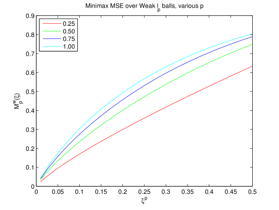
Figure 9: Minimax soft thresholding MSE over weak-$\ell_{p}$ balls, $M_{p}^{w}(\xi)$, for various $p$. Vertical axis: worst case MSE over ${\cal F}_{p}^{w}(\xi)$. Horizontal axis: $\xi^{p}$. Red, green, blue, aqua curves (from bottom to top) correspond to $p=0.25,0.50,0.75,1.00$.

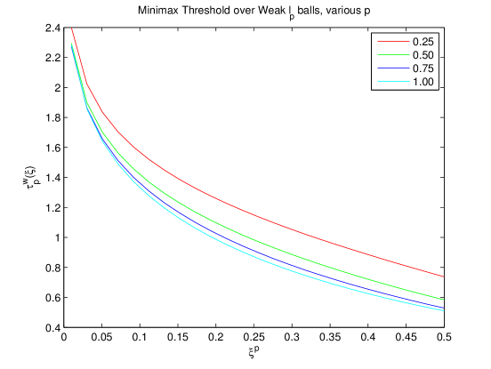
Figure 10: Minimax soft threshold parameter, $\tau_{p}^{w}(\xi)$, various $p$. Vertical axis: minimax threshold over ${\cal F}_{p}^{w}(\xi)$. Horizontal Axis: $\xi^{p}$. Red, green, blue, aqua curves (from top to bottom) correspond to $p=0.25,0.50,0.75,1.00$.

By a simple calculus exercise, this formula and Lemma 6.2, imply the following.

Lemma 6.3.

The function $M_{p}^{w}(\xi)$ is strictly monotone increasing in $\xi\in(0,\infty)$. Hence, the inverse function

$$(M_{p}^{w})^{-1}(m)=\inf\big{\{}\,\xi:\;M_{p}^{w}(\xi)\geq m\big{\}},$$

is well-defined for $m\in(0,1)$.

The asymptotic behavior of $M_{p}^{w}(\xi)$ in the very sparse limit $\xi\to 0$ was derived in [Joh93].

Lemma 6.4 ([Joh93]).

As $\xi\to 0$, the minimax threshold level achieving Eq. (6.14) is given by

$$\tau^{w}_{p}(\xi) = \sqrt{2\log(1/\xi^{p})}\cdot\{1+o(1)\}\,,\,,$$

and the corresponding minimax mean square error behaves, in the same limit, as

$$M^{w}_{p}(\xi)=\frac{2}{2-p}\,(2\log(1/\xi^{p}))^{1-p/2}\cdot\xi^{p}\cdot\{1+o(1)\}\,.$$ (6.16)

Comparing with Lemma 2.3, we see that the minimax threshold $\tau^{w}_{p}(\xi)$ coincides asymptotically with the one for strong $\ell_{p}$ balls. The corresponding risk is larger by a factor $2/(2-p)$ reflecting the larger set of possible distributions $\nu\in{\cal F}_{p}^{w}(\xi)$. For later use also note:

$$(M_{p}^{w})^{-1}(m)=\left(\frac{2-p}{p}m\right)^{1/p}\cdot\left(2\log(\frac{2-p}{p}m)^{-1})\right)^{1/2-1/p}\cdot(1+o(1)),\qquad m\rightarrow 0.$$

6.2 Minimax MSE in Compressed Sensing under Weak $p$-th Moments

We return now to the compressed sensing setup. In the noiseless case we consider sequences of instances ${\sf S}\equiv\{I_{n,N}\}=\{(x_{0}^{(N)},z^{(n)}=0,A^{(n,N)})\}_{n,N}$ in ${\cal S}_{p}^{w}(\delta,\xi,0)$. The minimax asymptotic mean square error of the LASSO is then given by considering the worst case sequence of instances

$$M_{p}^{w,*}(\delta,\xi)\equiv\sup_{{\sf S}\in{\cal S}_{p}^{w}(\delta,\xi,0)}\inf_{\lambda\in{\mathbb{R}}_{+}}{\rm AMSE}(\lambda;{\sf S})\,.$$ (6.17)

Here asymptotic mean-square error is defined as per Eq. (1.4).

Analogously, in the noisy case $\sigma>0$, we consider sequences of instances ${\sf S}\in{\cal S}_{p}^{w}(\delta,\xi,\sigma)$, We then define the minimax risk as

$$M_{p}^{w,*}(\delta,\xi,\sigma)\equiv\sup_{{\sf S}\in{\cal S}_{p}^{w}(\delta,\xi,\sigma)}\inf_{\lambda\in{\mathbb{R}}_{+}}{\rm AMSE}(\lambda;{\sf S})\,.$$ (6.18)

It turns out that complete analogs of the results of Sections 4 and 5 hold for the weak $p$-th moment setting. Since the proofs are easy modifications of the ones for strong $\ell_{p}$ balls, we omit them.

Theorem 6.1 (Noiseless Case, Weak $p$-th moment).

For $\delta\in(0,1)$, $\xi>0$, the Minimax AMSE of the LASSO over the weak-$\ell_{p}$ ball of radius $\xi$ is:

$$M_{p}^{w,*}(\delta,\xi)=\frac{\delta\xi^{2}}{(M_{p}^{w})^{-1}(\delta)^{2}}$$ (6.19)

where $(M_{p}^{w})^{-1}(\delta)$ is the inverse function of the soft thresholding minimax risk, see Eq. (6.14).

Further we have:

Least Favorable $\nu$. The least-favorable distribution $\nu^{w,*}$ is the most dispersed distribution $\nu_{p,\xi}$ whose distribution function is given by Eq. (6.10), with $\xi=\xi^{*}$.

Minimax Threshold. The minimax threshold $\lambda^{w,*}(\delta,\xi)$ is given by the calibration relation (3.4) with $\tau=\tau^{w,*}(\delta,\xi)$ determined by:

$$\tau^{w,*}(\delta,\xi)=\tau_{p}^{w}((M^{w}_{p})^{-1}(\delta))\,,$$ (6.20)

where $\tau_{p}^{w}(\,\cdot\,)$ is the soft thresholding minimax threshold, achieving the infimum in Eq. (6.14).

Saddlepoint. The pair $(\lambda^{w,*},\nu^{w,*})$ satisfies a saddlepoint relation. Put for short ${\rm AMSE}(\lambda;\nu)={\rm AMSE}(\lambda;\delta,\nu,\sigma=0)$. The minimax AMSE is given by

$$M^{w,*}_{p}(\delta;\xi)={\rm AMSE}(\lambda^{w,*};\nu^{w,*}),$$

and

$${\rm AMSE}(\lambda^{w,*};\nu^{w,*}) \leq {\rm AMSE}(\lambda;\nu^{w,*})\,,\qquad\forall\lambda>0$$ (6.21)

$$\geq {\rm AMSE}(\lambda^{w,*};\nu)\,,\qquad\forall\nu\in{\cal F}_{p}^{w}(\xi).$$ (6.22)

As an illustration of this theorem, consider again the limit $\delta=n/N\to 0$ after $N\to\infty$ (equivalently, $n/N\to 0$ sufficiently slowly). It follows from Eq. (6.16) that

$$M_{p}^{w,*}(\delta,1)=\Big{(}1-\frac{p}{2}\Big{)}^{-2/p}\delta^{1-2/p}(2\log(\delta^{-1}))^{2/p-1}\big{\{}1+o_{\delta}(1)\big{\}},\qquad\delta\rightarrow 0.$$

We can also compute the minimax regularization parameter. Lemma 6.4 gives

$$\lambda^{w,*}(\delta,\xi)=\xi\,\cdot\Big{(}1-\frac{p}{2}\Big{)}^{-1/p}\cdot\Big{(}\frac{2\log(1/\delta)}{\delta}\Big{)}^{1/p}\,\big{\{}1+o(1)\big{\}}\,,\quad\delta\to 0.$$ (6.23)

In the noisy case, we get a result in many respects similar to the $p$th moment result.

Theorem 6.2 (Noisy Case, Weak $p$-th moment).

For any $\delta,\xi>0$, let $m^{*}=m_{p}^{w,*}(\delta,\xi)$ be the unique positive solution of

$$\frac{m^{*}}{1+m^{*}/\delta}=M^{w}_{p}\left(\frac{\xi}{(1+m^{*}/\delta)^{1/2}}\right)\,.$$ (6.24)

Then the LASSO minimax mean square error $M_{p}^{w,*}$ is given by:

$$M_{p}^{w,*}(\delta,\xi,\sigma)=\sigma^{2}m^{w,*}_{p}(\delta,\xi/\sigma)\,.$$ (6.25)

Further, denoting by $\xi^{*}\equiv(1+m^{*}/\delta)^{-1/2}\xi/\sigma$, we have:

Least Favorable $\nu$. The least-favorable distribution $\nu^{w,*}$ is the most dispersed distribution $\nu_{p,\xi}$ whose distribution function is given by Eq. (6.10).

Minimax Threshold. The minimax threshold $\lambda^{*}(\delta,\xi,\sigma)$ is given by the calibration relation (3.4) with $\tau=\tau^{*}(\delta,\xi,\sigma)$ determined as follows:

$$\tau^{w.*}(\delta,\xi,\sigma)=\tau^{w}_{p}(\xi^{*}).$$ (6.26)

where $\tau_{p}^{w}(\,\cdot\,)$ is the soft thresholding minimax threshold, achieving the infimum in Eq. (6.14).

Saddlepoint. The above quantities obey a saddlepoint relation. Put for short ${\rm AMSE}(\lambda;\nu)={\rm AMSE}(\lambda;\delta,\nu,\sigma)$. The minimax AMSE obeys

$$M^{w,*}_{p}(\delta,\xi)={\rm AMSE}(\lambda^{w,*};\nu^{w,*})\,,$$

and

$${\rm AMSE}(\lambda^{*};\nu^{*}) \leq {\rm AMSE}(\lambda;\nu^{w,*})\,,\qquad\forall\lambda>0$$ (6.27)

$$\geq {\rm AMSE}(\lambda^{w,*};\nu)\,,\qquad\forall\nu\in{\cal S}^{w}_{p}(\xi).$$ (6.28)

7 Traditionally-scaled $\ell_{p}$-norm Constraints

This paper uses a non-traditional scaling $\|x_{0}\|_{p}^{p}\leq N\cdot\xi^{p}$ for the radius of $\ell_{p}$ balls; traditional scaling would be $\|x_{0}\|_{p}^{p}\leq\xi^{p}$. In this section we discuss the translation between the two types of conditions. We first define sequence classes based on norm constraints.

Definition 7.1.

The traditionally-scaled $\ell_{p}$ problem suite $\tilde{{\cal S}}_{p}(\delta,\xi,0)$ is the class of sequences of problem instances $I_{n,N}=(x_{0}^{(N)},z^{(n)},A^{(n,N)})$ where:
(1) $n/N\rightarrow\delta$;
(2) $\|x_{0}^{(N)}\|_{p}^{p}\leq\xi^{p}$, and, for some sequence $B=\{B_{M}\}_{M\geq 0}$ such that $B_{M}\to 0$, we have $\sum_{i=1}^{N}(x_{0,i}^{(N)})^{2}{\mathbb{I}}(|x_{0,i}^{(N)}|\geq M)\leq B_{M}N^{1-2/p}$ for every $N$;
(3) $z^{(n)}\in{\bf R}^{n}$, $\|z^{(n)}\|_{2}\sim\sigma\cdot n^{1/2}\cdot N^{-1/p}$, $(n,N)\rightarrow\infty$.
(4) $A^{(n,N)}\sim\mbox{\sc Gauss}(n,N)$.

The traditionally-scaled weak $\ell_{p}$ problem suite $\tilde{{\cal S}}_{p}^{w}(\delta,\xi,0)$ is defined using conditions (1),(3),(4) and
$(2^{w})$ $\|x_{0}^{(N)}\|_{w\ell_{p}}^{p}\leq\xi^{p}$, and, , for some sequence $B=\{B_{M}\}_{M\geq 0}$ such that $B_{M}\to 0$, we have $\sum_{i=1}^{N}(x_{0,i}^{(N)})^{2}{\mathbb{I}}(|x_{0,i}^{(N)}|\geq M)\leq B_{M}N^{1-2/p}$ for every $N$;

Comparing our earlier definitions of standard $\ell_{p}$-constrained problem suites ${\cal S}_{p}(\delta,\xi,\sigma)$ and ${\cal S}_{p}^{w}(\delta,\xi,\sigma)$ with these new definitions, conditions (1) and (4) are identical; while the new (2) and (3) are simply rescaled versions of corresponding conditions (2) and (3) in the earlier standard problem suites. To deal with such rescaling, we need the following scale covariance property:

Lemma 7.1.

Let $I=(x_{0}^{(N)},z^{(n)},A^{(n,N)})$ be a problem instance and $I_{a}=(a\cdot x_{0}^{(N)},a\cdot z^{(n)},A^{(n,N)})$ be the corresponding dilated problem instance. Suppose that $\hat{x}_{\lambda}^{(N)}$ is the unique LASSO solution generated by instance $I$ and $\hat{x}_{\lambda}^{(N),a}$ the unique solution generated by instance $I_{a}$. Then

$$\hat{x}_{a\lambda}^{(N),a}=a\cdot\hat{x}_{\lambda}^{(N)},$$

$$\|\hat{x}_{a\lambda}^{(N),a}-ax_{0}^{(N)}\|_{2}^{2}=a^{2}\cdot\|\hat{x}_{\lambda}^{(N)}-x_{0}^{(N)}\|_{2}^{2},$$

and

$$\inf_{\lambda}E\|\hat{x}_{\lambda}^{(N),a}-ax_{0}^{(N)}\|_{2}^{2}=a^{2}\cdot\inf_{\lambda}E\|\hat{x}_{\lambda}^{(N)}-x_{0}^{(N)}\|_{2}^{2}.$$

Applying this lemma yields the following problem equivalences:

Corollary 7.1.

We have the scaling relations:

$$\sup_{{\sf S}\in\tilde{{\cal S}}_{p}(\delta,\xi,0)}\inf_{\lambda}{\rm AMSE}(\lambda,{\sf S})=N^{-2/p}\cdot\sup_{{\sf S}\in{{\cal S}}_{p}(\delta,\xi,0)}\inf_{\lambda}{\rm AMSE}(\lambda,{\sf S});$$

and

$$\sup_{{\sf S}\in\tilde{{\cal S}}_{p}^{w}(\delta,\xi,0)}\inf_{\lambda}{\rm AMSE}(\lambda,{\sf S})=N^{-2/p}\cdot\sup_{{\sf S}\in{{\cal S}}_{p}^{w}(\delta,\xi,0)}\inf_{\lambda}{\rm AMSE}(\lambda,{\sf S}).$$

Let’s apply this to noiseless $\ell_{p}$ ball constraint. By Theorem 4.1 we have

$$\min_{\lambda}\max_{{\sf S}\in{\cal S}(\delta,\xi,0)}{\rm AMSE}(\lambda,{\sf S})=\frac{\delta\xi^{2}}{M_{p}^{-1}(\delta)^{2}}$$

Considering the unnormalized squared error $\|\widehat{x}_{\lambda}-x_{0}\|^{2}$ and operating purely formally, define a symbol $\bar{E}$ so that when $x_{0}^{(N)}$ arises from a given sequence ${\sf S}$,

$$\bar{E}\|\widehat{x}_{\lambda}^{(N)}-x_{0}^{(N)}\|^{2}=N\cdot{\rm AMSE}(\lambda,{\sf S}).$$

Remembering $\delta=n/N$ we have

$$\min_{\lambda}\max_{{\sf S}\in{{\cal S}}_{p}(\delta,\xi,0)}\bar{E}\|\widehat{x}_{\lambda}^{(N)}-x_{0}^{(N)}\|^{2} = N\cdot(n/N)^{1-2/p}\cdot\xi^{2}\cdot\left(2\log(N/n)\right)^{2/p-1}\big{\{}1+o_{N}(1)\big{\}}\,.$$

$$= N^{2/p}\xi^{2}\cdot\left(\frac{2\log(N/n)}{n}\right)^{2/p-1}\big{\{}1+o_{N}(1)\big{\}}.$$

Using the traditionally-scaled $\ell_{p}$ problem suite,

$$\min_{\lambda}\max_{{\sf S}\in\tilde{{\cal S}}_{p}(\delta,\xi,0)}\bar{E}\|\widehat{x}_{\lambda}-x_{0}\|^{2}=N^{-2/p}\cdot\min_{\lambda}\max_{{\sf S}\in{{\cal S}}_{p}(\delta,\xi,0)}\bar{E}\|\widehat{x}_{\lambda}-x_{0}\|^{2},$$

where on the LHS we have $\tilde{{\cal S}}_{p}(\delta,\xi,0)$ while on the RHS we have ${{\cal S}}_{p}(\delta,\xi,0)$. We conclude

Corollary 7.2.

Consider the noiseless, traditionally-scaled $\ell_{p}$ problem formulation. The asymptotic MSE for the $\ell^{2}$-norm error measure has the asymptotic form

$$\min_{\lambda}\max_{{\sf S}\in\tilde{{\cal S}}_{p}(\delta,\xi,0)}\bar{E}\|\widehat{x}_{\lambda}-x_{0}\|^{2}=\xi^{2}\cdot\left(\frac{2\log(N/n)}{n}\right)^{2/p-1}\big{\{}1+o_{N}(1)\big{\}};$$ (7.1)

this is valid both for $n/N\rightarrow\delta\in(0,1)$ and for $\delta=n/N\to 0$ slowly enough. The maximin penalization has an elegant prescription when $n/N\to 0$ slowly enough:

$$\lambda^{*}=\xi\cdot\left(\frac{2\log(N/n)}{n}\right)^{1/p},\qquad{\sf S}\in\tilde{{\cal S}}_{p}(\delta,\xi,0).$$ (7.2)

Our results can now be compared with earlier results written in the traditional scaling. We rewrite our result for $\xi=1$, using a simple moment condition that implies uniform integrability. For all sufficiently large $B$, and all $q>2$, we obtained:

$$\min_{\lambda}\max_{\|x_{0}\|_{p}^{p}\leq 1\,,\;\|x_{0}\|^{q}_{q}\leq BN^{1-q/p}}\bar{E}\|\widehat{x}_{\lambda}^{(N)}-x_{0}^{(N)}\|^{2}=\left(\frac{2\log(N/n)}{n}\right)^{2/p-1}\big{\{}1+o_{N}(1)\big{\}}.$$ (7.3)

In the case $\lambda=0$, earlier results [Don06a, CT05] imply:

$$\max_{\|x_{0}\|_{p}^{p}\leq 1}\|\widehat{x}_{0}-x_{0}\|^{2} = O_{P}\left(\Big{(}\frac{\log(N/n)}{n}\Big{)}^{2/p-1}\right),\;\;\;\;\;n/N\rightarrow 0.$$ (7.4)

There are two main differences in technical content between the new result and earlier ones

• The use of $\bar{E}$ on the LHS of (7.3) versus $O_{P}(\,\cdot\,)$ on the RHS of (7.4).

• The supremum over $\{\|x_{0}^{(N)}\|_{p}^{p}\leq 1\}$ on the LHS of (7.4) versus the supremum over $\{\|x_{0}^{(N)}\|_{p}^{p}\leq 1\}\cap\{\|x_{0}\|_{q}^{q}\leq BN^{1-q/p}\}$ on the LHS of (7.3).

The main difference in results is of course that the new result gives a precise constant in place of the $O(\,\cdot\,)$ result which was previously known. See Section 10.3 for further discussion.

The new result has the additional ingredient, not seen earlier, that we constrain not only $\{\|x_{0}^{(N)}\|_{p}^{p}\leq 1\}$ but also $\{\|x_{0}^{(N)}\|_{2}^{2}\leq BN^{1-q/p}\}$. For each $p<2$, this additional constraint does indeed give a smaller set of feasible vectors for large $N$. See Section 10.2 for further discussion.

A traditionally-scaled weak-$\ell_{p}$ problem suite $\tilde{{\cal S}}_{p}^{w}(\delta,\xi,\sigma)$ can also be defined; without giving details, we have:

Corollary 7.3.

Consider the noiseless, traditionally-scaled weak-$\ell_{p}$ problem formulation. The asymptotic MSE for the $\ell^{2}$-norm error measure has the asymptotic form

$$\min_{\lambda}\max_{{\sf S}\in\tilde{{\cal S}}_{p}^{w}(\delta,\xi,0)}\bar{E}\|\widehat{x}_{\lambda}-x_{0}\|^{2}=(1-p/2)^{-2/p}\cdot\xi^{2}\cdot\left(\frac{2\log(N/n)}{n}\right)^{2/p-1}\big{\{}1+o_{N}(1)\big{\}};$$ (7.5)

this is valid both for $n/N\rightarrow\delta\in(0,1)$ and for $\delta=n/N\to 0$ slowly enough. The maximin penalization has an elegant prescription for $n/N$ small:

$$\lambda^{*}=(1-p/2)^{-1/p}\cdot\xi\cdot\left(\frac{2\log(N/n)}{n}\right)^{1/p},\qquad{\sf S}\in\tilde{{\cal S}}_{p}^{w}(\delta,\xi,0).$$ (7.6)

8 Compressed Sensing over the Bump Algebra

Our discussion involving $\ell_{p}$-balls is so far rather abstract. We consider here a stylized application: recovering a signal $f$ in the Bump Algebra from compressed measurements. Consider a function $f:[0,1]\to{\mathbb{R}}$ which admits the representation

$$f(t)=\sum_{i=1}^{\infty}c_{i}\,g\big{(}(t-t_{i})/\sigma_{i}\big{)}\,,\;\;\;\;\;\;\;\;g(x)=\exp\big{(}-x^{2}/2\big{)},\quad\,\sigma_{i}>0.$$ (8.1)

Each term $g(\,\cdot\,)$ is a Gaussian ‘bump’ normalized to height 1, and we assume $\sum_{i=1}^{\infty}|c_{i}|\leq 1$ which ensures convergence of the series. The $c_{i}$ are signed amplitudes of the ‘bumps’ in $f$. We refer to the book by Yves Meyer [Mey84] and also to the discussion in [DJ98], which calls such objects models of polarized spectra. Any such function also has a wavelet representation

$$f=\sum_{j\geq-1}\sum_{k\in{\cal I}_{j}}\alpha_{j,k}\psi_{j,k},$$

where the $\psi_{j,k}$ are smooth orthonormal wavelets (for example Meyer wavelets or Daubechies wavelets), and the wavelet coefficients obey $\sum_{j,k}|\alpha_{j,k}|\leq C$. The constant $C$ depends only on the wavelet basis [Mey84]. Here $j$ denotes the level index, and $k$ the position index. We have $|{\cal I}_{-1}|=1$, and $|{\cal I}_{j}|=2^{j}$ for each $j\geq 0$. In other words the collection of functions with wavelet coefficients in an $\ell_{1}$-ball of radius $C$ contains the whole algebra of functions representable as in (8.1).

Now consider compressed sensing of such an object. We fix a maximum resolution, by picking $N=2^{J}$ and considering the finite-dimensional problem of recovering the object $f_{N}=\sum_{j<J}\sum_{k=0}^{2^{j}-1}\alpha_{j,k}\psi_{j,k}$. The scale $2^{-J}$ corresponds to an effective discretization scale: on intervals of length much smaller than $2^{-J}$, the function $f_{N}$ is approximately constant. Reconstructing the function $f_{N}$ is equivalent to recovering the $2^{J}$ coefficients

$$x_{0}=\left(\alpha_{-1,0},\alpha_{0,0},\alpha_{1,0},\alpha_{1,1},\alpha_{2,0},\dots,\alpha_{2,3},\alpha_{3,1},\dots,\alpha_{J-1,0},\dots,\alpha_{J-1,2^{J-1}-1}\right).$$

We know that coefficients at scales $1$ through $J-1$ combined have a total $\ell_{1}$-norm bounded by a numerical constant $C$. Without loss of generality, we shall take $C=1$ (this corresponds to rescaling the constraint on the bump representation (8.1)).

Denote by $V_{J}$ the $2^{J}$-dimensional space of functions on $[0,1]$, with resolution $2^{-J}$, i.e.

$$V_{J}\equiv\Big{\{}\sum_{j<J}\sum_{k=0}^{2^{j}-1}\alpha_{j,k}\psi_{j,k}:\;\;\alpha_{j,k}\in{\mathbb{R}}\Big{\}}\,.$$ (8.2)

We can construct a random linear measurement operator ${\cal A}:V_{J}\to{\mathbb{R}}^{n}$, such that the matrix $A$ representing ${\cal A}$ in the basis of wavelets has random Gaussian coefficients iid ${\sf N}(0,1)$. We then take $n+1$ noiseless measurements: the scalar $\alpha_{-1,0}=\langle f,\psi_{-1,0}\rangle$ associated to the ‘father wavelet’, and the vector $y={\cal A}f_{N}$. Notice that, since the measurements are noiseless, the variance of the entries of the measurement matrix $A$ can be rescaled arbitrarily.

In the wavelet basis, the measurements can be rewritten as $y=Ax_{0}$, where the $A$ is an $n\times N$ Gaussian random matrix. This is precisely a problem of the type studied in earlier sections. Suppose now that we apply $\ell_{1}$-penalized least-squares

$$\widehat{x}_{\lambda}\equiv\arg\min_{x}\Big{\{}\frac{1}{2}\|y-Ax\|_{2}^{2}+\lambda\|x\|_{1}\Big{\}}\,,$$ (8.3)

and denote the entries of the reconstruction vector by $\widehat{x}_{\lambda}\equiv(\widehat{\alpha}_{0,0},\dots,\widehat{\alpha}_{J-1,2^{J-1}-1})$. The function $f_{N}$ is therefore reconstructed as $\widehat{f}_{N}$, where

$$\widehat{f}_{N}=\sum_{j<J}\sum_{k=0}^{2^{j}-1}\hat{\alpha}_{j,k}\psi_{j,k}\,.$$

We adopt the performance measure

$${\rm MSE}(\widehat{f}_{N},f_{N})\equiv{\mathbb{E}}\big{\{}\|f_{N}-\widehat{f}_{N}\|_{L_{2}[0,1]}^{2}\big{\}}={\mathbb{E}}\|x_{0}-\widehat{x}_{\lambda}\|_{2}^{2};$$

where the last equality uses the orthonormality of the wavelet basis.

We wish to choose an appropriate value of $\lambda\geq 0$ to give the best reconstruction performance. Note that the coefficients vector $x_{0}\in{\mathbb{R}}^{N}$ satisfies by assumption

$$\|x_{0}\|_{1}\leq 1\,$$

so we are in the setting of traditionally-scaled $\ell_{p}$ balls. The discussion of the last section now applies; we obtain results by rescaling results from Theorem 4.1. Letting $\lambda_{p}^{*}(\delta,\xi)$ denote the minimax threshold of Theorem 4.1, define

$$\lambda_{N}=N^{-1}\cdot\lambda_{1}^{*}(\frac{n}{N},1).$$ (8.4)

Corollary 8.1.

Consider a sequence of functions $f_{N}\in V_{J}$ in the Bump Algebra (normed so that the wavelet coefficients have $\ell_{1}$-norm bounded by $1$). Consider Gaussian measurement operators ${\cal A}_{N}:V_{J}\to{\mathbb{R}}^{n}$ indexed by the problem dimensions $N=2^{J}$, and $n$. Let $\widehat{f}_{N}^{*}$ denote the reconstruction of $f_{N}$ using regularization parameter $\lambda=\lambda_{N}$ of (8.4).

(i) Assume $n/N\to\delta\in(0,1)$. Then we have

$${\rm MSE}(\widehat{f}_{N}^{*},f_{N})\leq N^{-1}\cdot M_{1}^{*}(\delta,1)\,(1+o(1))\,,$$ (8.5)

with $M_{1}^{*}(\delta,\xi)$ as in Theorem 4.1. This bound is asymptotically tight (achieved for a specific sequence $f_{N}$).

(ii) Assume $n/N\to 0$ sufficiently slowly. Then we have

$${\rm MSE}(\widehat{f}_{N}^{*},f_{N})\leq{\frac{2\log(N/n)}{n}}\cdot(1+o(1)),\,,$$ (8.6)

and the bound is asymptotically tight (achieved for a specific sequence $f_{N}$).

9 Compressed Sensing over Bounded Variation Classes

Compressed sensing problems make sense for many other functional classes. The class of Bounded Variation affords an application of our results on weak $\ell_{p}$ classes.

1. Every bounded variation function $f\in BV[0,1]$ has Haar wavelet coefficients in a weak-$\ell_{2/5}$ ball.

2. Every $f\in BV[0,1]^{2}$ has wavelet coefficients in a weak-$\ell_{1}$ ball [CDPX99].

We can develop a theory of compressed sensing over BV spaces following the previous section, now using Haar wavelets. $V_{J}$ means again the span wavelets of spatial scale $2^{-J}$ or coarser. We let $d$ denote the spatial dimension ($d=1$ or $2$ in the above examples). We use regularization parameter

$$\lambda_{N}=N^{-1}\cdot\lambda^{w,*}(n/N,1).$$ (9.1)

Corollary 9.1.

Consider a sequence of functions $f_{N}\in V_{J}$ whose Haar wavelet coefficients have weak $\ell_{p}$-norm bounded by $1$. Consider Gaussian measurement operators ${\cal A}_{N}:V_{J}\to{\mathbb{R}}^{n}$ indexed by the problem dimensions $N=2^{dJ}$, and $n$. Let $\widehat{f}_{N}^{*}$ denote the reconstruction of $f_{N}$ using regularization parameter $\lambda=\lambda_{N}$ of (9.1).

(i) Assume $n/N\to\delta\in(0,1)$. Then we have

$${\rm MSE}(\widehat{f}_{N}^{*},f_{N})\leq N^{-1}\cdot M_{p}^{w,*}(\delta,1)\,(1+o(1))\,,$$ (9.2)

with $M_{1}^{*,w}(\delta,\xi)$ as in Theorem 6.1. This bound is asymptotically tight (achieved for a specific sequence $f_{N}$).

(ii) Assume $n/N\to 0$ sufficiently slowly. Then we have

$${\rm MSE}(\widehat{f}_{N}^{*},f_{N})\leq\Big{(}1-\frac{p}{2}\Big{)}^{-2/p}\cdot\left({\frac{2\log(N/n)}{n}}\right)^{2/p-1}\cdot(1+o(1)),\,,$$ (9.3)

and the bound is asymptotically tight (achieved for a specific sequence $f_{N}$).

Although BV offers only the applications $p=1$ ($d=2$) and $p=2/5$ ($d=1$), weak-$\ell_{p}$ spaces arise elsewhere, and serve as useful models for image content. For example, for images containing smooth edges, we have the following model: every $f:[0,1]^{2}\mapsto{\mathbb{R}}$ which is locally in $C^{2}$ except at $C^{2}$ ‘edges’ has curvelet coefficients levelwise in weak-$\ell_{2/3}$ balls [CD04]. Our compressed sensing result for BV can be adapted without change to the conclusions for such a setting, after replacing the role of Haar wavelets by Curvelets.

10 Discussion

In this last section we discuss some specific aspects of our results and overview (in an unavoidably incomplete way) the related literature.

10.1 Equivalence of Random and Deterministic Signals/Noises

A striking aspect of our results is the equivalence of random and deterministic signals and noises (traceable here to Proposition 3.1). The AMSE formula in the general case, as given by Eq. (3.5), depends on the sequence of signals $x_{0}^{(N)}$ and of noise vectors $z^{(n)}$ only through simple statistics of such vectors. More precisely, it depends only on their asymptotic empirical distributions, respectively $\nu$ and $\omega$. In fact the dependence on $z^{(n)}$ is even weaker: the asymptotic risk only depends on the limit second moment ${\mathbb{E}}_{\omega}(Z^{2})$.

At first sight, these findings are somewhat surprising. For instance we might replace $x_{0}^{(N)}$ with a random vector with i.i.d. entries with common distribution $\nu$ without changing the asymptotic risk. This asymptotic equivalence between random and deterministic signal is in fact a quite simple and robust consequence of the absence of structure of the measurement matrix $A$. We do not spell out the details here, but note the following simple facts

1. Under our model for $A$, the columns of $A$ are exchangeable, so there is no distributional difference between $Ax_{0}$ and $APx_{0}$, for any permutation matrix $P$.

2. As a consequence, there is no difference in expected performance between a fixed vector $x_{0}$ and a random vector obtained by permuting the entries of $x_{0}$ uniformly at random.

3. Asymptotically for large $N$ there is a negligible difference in performance between a fixed vector $x_{0}$ and the typical random vector obtained by sampling with replacement from the entries of $x_{0}$.

This argument implies that we can replace the deterministic vectors $x_{0}^{(N)}$ with random vectors with i.i.d. entries. As the argument clarifies, this phenomenon ought to exist for more general models of $A$.

10.2 Comparison with Previous Approaches

Much of the analysis of compressed sensing reconstruction methods has relied so far on a kind of qualitative analysis. A typical approach has been to frame the analysis in terms of ‘worst case’ conditions on the measurement matrix $A$. A useful set of conditionsis provided by the restricted isometry property (RIP), [CT05, CRT06] and refinements [BRT09, vdGB09, BGI⁺08]. These conditions are typically pessimistic, in that they assume that the signal $x_{0}$ is chosen adversarially, but they capture the correct scaling behavior.

The advantage of this approach is its broad applicability; since one assumes little about the matrix $A$, the derived bound will perhaps apply to a wide range of matrices. However, there are two limitations:

1. These conditions have been proved to hold with linear scaling of $\|x_{0}\|$ and $n$ with the signal dimension $N$, only for specific random ensembles of measurement matrices, e.g. random matrices with i.i.d. subexponential entries.

2. The resulting bounds typically only hold up to unspecified numerical constants. Efforts to make precise the implied constants in specific cases (see for instance [BCT11]) show that this approach imposes restrictive conditions on the signal sparsity. For instance, for a Gaussian measurement matrix with undersampling ratio $\delta=0.1$, RIP implies successful reconstruction [BCT11] only if $\|x_{0}\|_{0}\lesssim 0.0002\,N$. In empirical studies, a much larger support appears to be tolerated.

The present paper works with only one matrix ensemble – Gaussian random matrices – but gets quantitatively precise results, like the companion works [DMM09, DMM10, BM10]. The approach provides sharp performance guarantees under suitable probabilistic models for the measurement process.

To be concrete, consider the case of $x_{0}$ belonging to the weak-$\ell_{p}$ ball of radius $1$, $\|x_{0}\|_{w\ell_{p}}\leq 1$. Building on the RIP theory, the review paper [Can06] derives the bound

$$\|\widehat{x}_{\lambda}-x_{0}\|^{2} \leq C\,\left(\frac{\log(N/n)}{n}\right)^{2/p-1}\,,$$ (10.1)

holding for Gaussian measurement matrices $A$, and for unspecified constant $C$. Analogous minimax bounds for $\ell_{p}$ balls are known [Don06a, RWY09]. Our results have the same form, but with specific constants, e.g. $C=(1-(p/2))^{-2/p}$ for weak-$\ell_{p}$ balls, cf. Eq. (7.5) and $C=1$ for ordinary $\ell_{p}$ balls, cf. Eq. (7.1). Moreover, these constants are sharp, i.e. attained by specifically described $x_{0}$.

Let us finally mention the recent paper [CP10], that takes a probabilistic point of view similar to the one of [DMM10] and to the present one, although using different techniques. This approach avoids using RIP or similar conditions, and applies to a broad family of matrices with i.i.d. rows. On the other hand, it only allows to prove upper bounds on MSE off by logarithmic factors.

10.3 Comparison to the theory of widths

Recall that the Gel’fand $n$-width of of a set $K\subseteq{\mathbb{R}}^{N}$ with respect to the norm $\|\,\cdot\,\|_{X}$ is defined as

$$d_{n}(K,X)=\inf_{A\in{\mathbb{R}}^{n\times N}}\sup_{x\in K\cap\text{ker}(A)}\|x\|_{X}\,,$$ (10.2)

where $\text{ker}(A)\equiv\{v\in{\mathbb{R}}^{N}:\,Av=0\}$. Here we shall consider $K$ to be the $\ell_{p}$ ball of radius $1$, $B_{p}^{N}\equiv\{x\in{\mathbb{R}}^{N}\,:\;\|x\|_{p}\leq 1\}$, and fix $\|\,\cdot\,\|_{X}$ to be the ordinary $\ell_{2}$ norm. A series of works [Kas77, GG84, Don06a, FPRU10] established that

$$d_{n}(B_{p}^{N},\ell_{2})\geq c_{p}\left(\frac{\log(N/n)}{n}\right)^{1/p-1/2}$$ (10.3)

as long as the term in parenthesis is smaller than $1$.

The interest for us lies in the well-known observation [Don06a] that $d_{n}(B_{p}^{N},\ell_{2})$ provides a lower bound on the compressed sensing mean square error under arbitrary reconstruction algorithm, and for arbitrary measurement matrix $A$. In particular

$$\max_{x_{0}\in B_{p}^{N}}\|\widehat{x}-x_{0}\|\geq d_{n}(B_{p}^{N},\ell_{2})\,.$$ (10.4)

So it makes sense to define the inefficiency of a certain matrix/reconstruction procedure as the ratio of the two sides in the above inequality

$$r_{\rm alg}(B_{p}^{N},\ell_{2})\equiv\frac{1}{d_{n}(B_{p}^{N},\ell_{2})}\max_{x_{0}\in B_{p}^{N}}\|\widehat{x}-x_{0}\|\,.$$ (10.5)

This ratio implicitly depends on the matrix $A$. In the case $p=1$, $\lambda=0$ it is known that $\ell^{1}$ minimization is inefficient at most by a factor $2$:

$$r_{{\rm min}\;\ell_{1}}(B_{p}^{N},\ell_{2})\leq 2;$$ (10.6)

(for example [Don06a] showed this by invoking [TW80]).

Our work concerns random Gaussian matrices and LASSO reconstruction. Since the worst-case performance of the optimally-tuned LASSO can not be worse than the worst-case performance of min-$\ell^{1}$ reconstruction, and since we have a formal expression for the worst-case AMSE of optimally-tuned LASSO, the asymptotic formula (7.1) together with the bound (10.3) implies for all sufficiently large $B$ and any $q>2$ that

$$\max_{x_{0}\in B_{p}^{N},\;\|x_{0}\|_{q}\leq BN^{1/q-1/p}}\overline{E}\|\widehat{x}_{0}^{(N)}-x_{0}\|=\sqrt{\frac{2\log(N/n)}{n}}(1+o(1)),$$ (10.7)

with $\overline{E}$ defined in analogy with Section 7. The constant $B$ is arbitrary, which suggests (but of course does not prove) that we can remove the hypothesis $\|x_{0}\|_{q}\leq BN^{1/q-1/p}$ completely.

On the other hand, for a fixed matrix $A\in{\mathbb{R}}^{n\times N}$, we can define the width

$$d_{n}(K,A,X)=\sup_{x\in K\cap\text{ker}(A)}\|x\|_{X}\,,$$

so that the Gel’fand $n$-width is the infimum of this quantity over $A$. Using results of Donoho and Tanner [DT10] one can give the lower bound for $p=1$ and Gaussian random matrices

$$d_{n}(B_{p}^{N},A,\ell_{2})\geq\sqrt{\frac{\log(N/n)}{4en}}(1+o(1)).$$

The right hand side of Eq. (10.7) is quantitatively quite close to the right-hand side of the last display. Hence the results of this paper suggest that statistical methods may also provide geometric information.

In the general case $0<p<1$, lower bounds on $c_{p}$ are given in [FPRU10], but they do not appear as tight as desirable.

10.4 About the Uniform Integrability Condition

We have just seen once again that our hypotheses on $\ell_{p}$ balls can be scaled to match $\|x_{0}\|_{p}\leq 1$ but then they also include the hypothesis $\|x_{0}\|_{q}\leq BN^{1/q-1/p}$. It may seem at first glance that this is a serious additional constraint; it implies that the entries in $x_{0}$ cannot be very large as $N$ increases, whereas the condition $\|x_{0}\|_{p}\leq 1$ of course permits entries as large as 1.

However, note that our analysis identifies the least-favorable $x_{0}$, and that the constant $B$ plays no role. In fact, if we make a homotopy between the least-favorable object and objects requiring larger $B$, we find that the AMSE is decreasing in the direction of larger $B$. Pushing things to the extreme where $B$ goes unbounded, of course our analysis techniques no longer rigorously apply, but it is quite clear that this is an unpromising direction to move. Hence we believe that this is largely a technical condition, caused by our method of proof.

References

- [BCT11] J. D. Blanchard, C. Cartis, and J. Tanner, Compressed sensing: How sharp is the restricted isometry property?, SIAM Review 53 (2011), 105–125.
- [BGI+08] R. Berinde, A.C. Gilbert, P. Indyk, H. Karloff, and M.J. Strauss, Combining geometry and combinatorics: A unified approach to sparse signal recovery, 47th Annual Allerton Conference (Monticello, IL), September 2008, pp. 798 – 805.
- [BM10] M. Bayati and A. Montanari, The LASSO risk for gaussian matrices, arXiv:1008.2581, 2010.
- [BM11] , The dynamics of message passing on dense graphs, with applications to compressed sensing, IEEE Trans. on Inform. Theory 57 (2011), 764–785.
- [BRT09] P. J. Bickel, Y. Ritov, and A. B. Tsybakov, Simultaneous analysis of Lasso and Dantzig selector, Amer. J. of Mathematics 37 (2009), 1705–1732.
- [Can06] E. Candès, Compressive sampling, Proceedings of the International Congress of Mathematicians (Madrid, Spain), 2006.
- [CD95] S.S. Chen and D.L. Donoho, Examples of basis pursuit, Proceedings of Wavelet Applications in Signal and Image Processing III (San Diego, CA), 1995.
- [CD04] E.J. Candès and DL Donoho, New tight frames of curvelets and optimal representations of objects with piecewise singularities, Comm. Pure Appl. Math 57 (2004), 219–266.
- [CDPX99] A. Cohen, R. DeVore, P. Petrushev, and H. Xu, Nonlinear Approximation and the Space BV, Amer. J. of Mathematics 121 (1999), 587–628.
- [CP10] E. Candés and Y. Plan, A probabilistic and RIPless theory of compressed sensing, arXiv:1011.3854, 2010.
- [CRT06] E. Candes, J. K. Romberg, and T. Tao, Stable signal recovery from incomplete and inaccurate measurements, Communications on Pure and Applied Mathematics 59 (2006), 1207–1223.
- [CT05] E. J. Candes and T. Tao, Decoding by linear programming, IEEE Trans. on Inform. Theory 51 (2005), 4203–4215.
- [DJ94] D. L. Donoho and I. M. Johnstone, Minimax risk over balls, Prob. Th. and Rel. Fields 99 (1994), 277–303.
- [DJ98] , Minimax estimation via wavelet shrinkage, Annals of Statistics 26 (1998), 879–921.
- [DLM90] D.L. Donoho, R.C. Liu, and K.B. MacGibbon, Minimax risk over hyperrectangles, and implications, Annals of Statistics 18 (1990), 1416–1437.
- [DMM09] D. L. Donoho, A. Maleki, and A. Montanari, Message Passing Algorithms for Compressed Sensing, Proceedings of the National Academy of Sciences 106 (2009), 18914–18919.
- [DMM10] D.L. Donoho, A. Maleki, and A. Montanari, The Noise Sensitivity Phase Transition in Compressed Sensing, arXiv:1004.1218, 2010.
- [Don06a] D. L. Donoho, Compressed sensing, IEEE Transactions on Information Theory 52 (2006), 489–509.
- [Don06b] D. L. Donoho, High-dimensional centrally symmetric polytopes with neighborliness proportional to dimension, Discrete and Computational Geometry 35 (2006), no. 4, 617–652.
- [DT05] D. L. Donoho and J. Tanner, Neighborliness of randomly-projected simplices in high dimensions, Proceedings of the National Academy of Sciences 102 (2005), no. 27, 9452–9457.
- [DT10] , Counting faces of randomly projected polytopes when the projection radically lowers dimension, J. Amer. Math. Soc., 22 (2009), 1-53
- [DT10] , Precise undersampling theorems, Proc. IEEE 98 (2010), 913-924
- [DTDS06] D. L. Donoho, Y. Tsaig, I. Drori, and J.-L. Starck, Sparse solution of underdetermined linear equations by stagewise orthogonal matching pursuit, Stanford Tecnical Report, 2006.
- [FPRU10] S. Foucart, A. Pajor, H. Rauhut, and T. Ullrich, The Gelfand widths of -balls for , Journal of Complexity 26 (2010), 629–640.
- [GG84] A.Y. Garnaev and E.D. Gluskin, On widths of the euclidean ball, Soviet Mathematics Doklady 30 (1984), 200–203.
- [Joh93] I.M. Johnstone, Minimax bayes, asymptotic minimax and sparse wavelet priors, Statistical Decision Theory and Related Topics V, Springer-Verlag, 1993, pp. 303–326.
- [Kas77] B. Kashin, Diameters of Some Finite-Dimensional Sets and Classes of Smooth Functions, Math. USSR Izv. 11 (1977), 317–333.
- [LDSP08] M. Lustig, D.L Donoho, J.M. Santos, and J.M Pauly, Compressed sensing mri, IEEE Signal Processing Magazine (2008).
- [Mey84] Y. Meyer, Wavelets, Cambridge University Press, 1984.
- [RWY09] G. Raskutti, M. J. Wainwright, and B. Yu, Minimax rates of estimation for high-dimensional linear regression over -balls, 47th Annual Allerton Conference (Monticello, IL), September 2009.
- [Tib96] R. Tibshirani, Regression shrinkage and selection with the lasso, J. Royal. Statist. Soc B 58 (1996), 267–288.
- [TW80] J. F. Traub and H. Wozniakowski, A general theory of optimal algorithms, Academic Press, New York, 1980.
- [vdGB09] S. A. van de Geer and P. Bühlmann, On the conditions used to prove oracle results for the Lasso, Electron. J. Statist. 3 (2009), 1360–1392.