Continuations of the nonlinear Schrödinger equation beyond the singularity

Abstract

We present four continuations of the critical nonlinear Schrödinger equation (NLS) beyond the singularity: 1) a sub-threshold power continuation, 2) a shrinking-hole continuation for ring-type solutions, 3) a vanishing nonlinear-damping continuation, and 4) a complex Ginzburg-Landau (CGL) continuation. Using asymptotic analysis, we explicitly calculate the limiting solutions beyond the singularity. These calculations show that for generic initial data that leads to a loglog collapse, the sub-threshold power limit is a Bourgain-Wang solution, both before and after the singularity, and the vanishing nonlinear-damping and CGL limits are a loglog solution before the singularity, and have an infinite-velocity expanding core after the singularity. Our results suggest that all NLS continuations share the universal feature that after the singularity time $T_{c}$, the phase of the singular core is only determined up to multiplication by $e^{i\theta}$. As a result, interactions between post-collapse beams (filaments) become chaotic. We also show that when the continuation model leads to a point singularity and preserves the NLS invariance under the transformation $t\rightarrow-t$ and $\psi\rightarrow\psi^{\ast}$, the singular core of the weak solution is symmetric with respect to $T_{c}$. Therefore, the sub-threshold power and the shrinking-hole continuations are symmetric with respect to $T_{c}$, but continuations which are based on perturbations of the NLS equation are generically asymmetric.

1 Introduction

The focusing nonlinear Schrödinger equation (NLS)

$$i\psi_{t}(t,{\bf x})+\Delta\psi+|\psi|^{2\sigma}\psi=0,\qquad\psi_{0}(0,{\bf x})=\psi_{0}({\bf x})\in H^{1},$$ (1)

where ${\bf x}=(x_{1},...,x_{d})\in\mathbb{R}^{d}$ and $\Delta=\partial_{x_{1}x_{1}}+\cdot\cdot\cdot\partial_{x_{d}x_{d}}$, is one of the canonical nonlinear equations in physics, arising in various fields such as nonlinear optics, plasma physics, Bose-Einstein condensates (BEC), and surface waves. In the two-dimensional cubic case, this equation models the propagation of intense laser beams in a bulk Kerr medium. In that case, $\psi$ is the electric field envelope, $t$ is the direction of propagation, $d=2$, $x_{1}$ and $x_{2}$ are the transverse coordinates, and $\sigma=1$ (cubic nonlinearity).

In 1965, Kelley showed that the two-dimensional cubic NLS admits solutions that collapse (become singular) at a finite time (distance) $T_{c}$ [1]. Since physical quantities do not become singular, this implies that some of the terms that were neglected in the derivation of the NLS, become important near the singularity. Therefore, the standard approach for continuing the solution beyond the singularity has been to consider a more comprehensive model, in which the collapse is arrested.

In this study, we adopt a different approach, and ask whether singular NLS solutions can be continued beyond the singularity, within the NLS model. By this we mean that the solution satisfies the NLS both before and after the singularity, and a matching (”jump”) condition at the singularity. The motivation for this approach comes from hyperbolic conservation laws, where in the absence of viscosity, the solution can become singular (develop shocks). In that case, there is a huge body of literature on how to continue the inviscid solution beyond the singularity, which consists of Riemann problems, vanishing-viscosity solutions, entropy conditions, Rankine-Hogoniot jump conditions, specialized numerical methods, etc. In contrast, two studies from 1992 by Merle [2, 3], and a recent study by Merle, Raphael and Szeftel [4], addressed this question in the NLS. Tao [5] proved the global existence and uniqueness in the semi Strichartz class for solutions of the critical NLS. Intuitively, these solutions are formed by solving the equation in the Strichartz class whenever possible, and deleting any power that escapes to spatial or frequency infinity when the solution leaves the Strichartz class. These solutions, however, do not depend continuously on the initial conditions, and are thus not a well-posed class of solutions. Stinis [6] studied numerically the continuation of singular NLS solutions using the t-model approach.

In [2], Merle presented an explicit continuation of a singular NLS solution beyond the singularity, which is based on reducing the power ($L^{2}$ norm) of the initial condition of the explicit blowup solution $\psi_{\rm explicit,\alpha}$, see (8), below the critical power for collapse $P_{\rm cr}$. This continuation has two key properties:

1. Property 1: The solution is symmetric with respect to the singularity time $T_{c}$.

2. Property 2: After the singularity, the solution can only be determined up to multiplication by a constant phase term.

Merle’s breakthrough result, however, applies only to the critical NLS ($\sigma d=2$), and only to the explicit blowup solutions $\psi_{\rm explicit,\alpha}$. Recently, Merle, Raphael and Szeftel [4] generalized this result to Bourgain-Wang singular solutions [7], i.e., solutions that have a singular component that collapses as $\psi_{\rm explicit,\alpha}$, and a non-zero regular component that vanishes at the singularity point and does not participate in the collapse process.

In [3], Merle presented a different continuation, which is based on the addition of nonlinear saturation. This study showed that, generically, as the nonlinear saturation parameter goes to zero, the limiting solution can be decomposed beyond $T_{c}$ into two components: A $\delta$-function singular component with power $m(t)\geq P_{\rm cr}$, and a regular component elsewhere. Similar results follow from the asymptotic analysis of Malkin [8], which suggests that $m(t)\equiv P_{\rm cr}$ for $T_{c}\leq t<\infty$.

It is thus useful to distinguish between two types of continuations:

1. A point singularity, in which the weak solution is singular at $T_{c}$, but regular (i.e., in $H^{1}$) for $t>T_{c}$.

2. A filament singularity, in which the weak solution has a $\delta$-function singularity for $T_{c}\leq t\leq T_{0}$, where $T_{c}<T_{0}\leq\infty$. The motivation for this terminology comes from nonlinear optics, where collapsing beams can form long and narrow filaments (which, to leading order, can be viewed as an ”extended” $\delta$-function).

In this work we propose four novel continuations that lead to a point singularity, and obtain explicit formulae for the solution beyond the singularity. Our main findings are:

1. The non-uniqueness of the phase beyond the singularity (Property 2) is a universal feature of NLS continuations.

2. The symmetry with respect to the singularity time (Property 1) holds only if the continuation is time reversible and leads to a point singularity. Therefore, it is non-generic.

The paper is organized as follows. In section 2 we provide a short review of NLS theory. In section 3 we present Merle’s continuation of $\psi_{\rm explicit,\alpha}$, and illustrate it numerically. In section 4 we generalize this approach and present a sub-threshold power continuation, which can be applied to generic initial condition of the critical NLS. We compute asymptotically the limiting solution, and show that it is a Bourgain-Wang solution, both before and after the singularity. In particular, this continuation preserves the two key properties of Merle’s continuation. In section 5 we show that Property 1 (symmetry with respect to $T_{c}$) holds for time-reversible continuations that lead to a point singularity. In Section 6 we discuss the nonlinear-saturation continuation, which leads to a filament singularity. In section 7 we show that because of the phase non-uniqueness (Property 2), the interaction between post-collapse beams is chaotic. In section 8 we present a vanishing-hole continuation, which is suitable for ring-type singular solutions. This continuation is time-reversible, and it satisfies Properties 1 and 2. In section 9 we present a vanishing nonlinear-damping continuation, and compute the continuation asymptotically in two cases:

1. The nonlinear-damping continuation of the explicit solution $\psi_{\rm explicit,\alpha}$ is, up to an undetermined constant phase, given by $\psi_{\rm explicit,\kappa\alpha}$ with $\kappa\approx 1.614$.

2. The nonlinear-damping continuation of solutions that undergo a loglog collapse has an infinite-velocity expanding core, with an undetermined constant phase.

Therefore, the phase becomes non-unique beyond the singularity (Property 2). In contrast with previous continuations, however, the solution is asymmetric with respect to the singularity time (i.e., the solution does not satisfy Property 1). This is to be expected, as the nonlinear-damping continuation is not time-reversible. In Section 10 we show that the continuation which is based on the complex Ginzburg-Landau (CGL) limit of the NLS, is equivalent to the vanishing nonlinear-damping continuation. In section 11 we show a continuation of singular solutions of the linear Schrödinger equation. In this case, the limiting phase beyond the singularity is unique. This shows that the post-collapse non-uniqueness of the phase (Property 2) is a nonlinear phenomenon. Section 12 concludes with a discussion.

1.1 Level of rigor

The results which are derived in this manuscript are non-rigorous, and are based on asymptotic analysis, numerical simulations, and physical arguments. To emphasize this, we use the terminology Continuation Results, rather than Propositions or Theorems.

2 Review of NLS theory

We briefly review NLS theory, for more information see [9, 10, 11]. The NLS (1) has two important conservation laws: Power conservation

$$P(t)\equiv P(0),\qquad P(t)=\int|\psi|^{2}d{\bf x},$$

and Hamiltonian conservation

$$H(t)\equiv H(0),\qquad H(t)=\int|\nabla\psi|^{2}d{\bf x}-\frac{1}{\sigma+1}\int|\psi|^{2\sigma+2}d{\bf x}.$$ (2)

The NLS admits the waveguide solutions $\psi=e^{it}R(r)$, where $r=|{\bf x}|$, and $R$ is the solution of

$$R^{\prime\prime}(r)+\frac{d-1}{r}R^{\prime}-R+R^{2\sigma+1}=0,\qquad R^{\prime}(0)=0,\quad R(\infty)=0.$$ (3)

When $d=1$, the solution of (3) is unique, and is given by

$$R_{\sigma}(x)=(1+\sigma)^{1/2\sigma}\mbox{cosh}^{-1/\sigma}(\sigma x).$$ (4)

When $d\geq 2$, equation (3) admits an infinite number of solutions. The solution with the minimal power, which we denote by $R^{(0)}$, is unique, and is called the ground state.

When $\sigma d<2$, the NLS is called subcritical. In that case, all $H^{1}$ solutions exist globally. In contrast, both the critical NLS ($\sigma d=2$) and the supercritical NLS ($\sigma d>2)$ admit singular solutions.

Let $\psi(t,\bf x)$ be a solution of the NLS (1). Then, $\psi$ remains a solution of the NLS (1) under the following transformations:

1. Spatial translations: $\psi(t,{\bf x})\rightarrow\psi(t,{\bf x}+{\bf x}_{0})$, where ${\bf x}_{0}\in\mathbb{R}^{d}$.

2. Temporal translations: $\psi(t,{\bf x})\rightarrow\psi(t+t_{0},{\bf x})$, where $t_{0}\in\mathbb{R}$.

3. Phase change: $\psi(t,{\bf x})\rightarrow e^{i\theta}\psi(t,{\bf x})$, where $\theta\in\mathbb{R}$.

4. Dilation: $\psi(t,{\bf x})\rightarrow\lambda^{1/\sigma}\psi(\lambda^{2}t,\lambda{\bf x})$, where $\lambda\in\mathbb{R}^{+}$.

5. Galilean transformation: $\psi(t,{\bf x})\rightarrow\psi(t,{\bf x}-{\bf c}t)e^{i{\bf c}\cdot{\bf x}/2-i|{\bf c}|^{2}t/4}$, where ${\bf c}\in\mathbb{R}^{d}$.

Therefore, multiplying the initial condition by a constant phase $e^{i\theta}$ does not affect the solution. In addition, by the Galilean transformation, multiplying the initial condition by a linear phase term $\psi_{0}(x)\rightarrow\psi_{0}({\bf x})e^{i{\bf c}\cdot{\bf x}/2}$ does not affect the dynamics, but rather causes the solution to be tilted in the direction of ${\bf{n}}=(1,{\bf{c}})\in\mathbb{R}\times\mathbb{R}^{d}$.

2.1 Critical NLS

In the critical case $\sigma d=2$, equation (1) can be rewritten as

$$i\psi_{t}(t,{\bf x})+\Delta\psi+|\psi|^{4/d}\psi=0,\qquad\psi_{0}(0,{\bf x})=\psi_{0}({\bf x})\in H^{1},$$ (5)

and equation (3) can be rewritten as

$$R^{\prime\prime}(r)+\frac{d-1}{r}R^{\prime}-R+R^{4/d+1}=0,\qquad R^{\prime}(0)=0,\quad R(\infty)=0.$$ (6)

Theorem 1 (Weinstein [12]).

A sufficient condition for global existence in the critical NLS (5) is that $\|\psi_{0}\|_{2}^{2}<P_{\rm cr}$, where $P_{\rm cr}=\|R^{(0)}\|_{2}^{2}$, and $R^{(0)}$ is the ground state of equation (6).

The critical NLS (5) admits the explicit solution

$$\psi_{\rm explicit}(t,r)=\frac{1}{L^{d/2}(t)}R^{(0)}\left(\frac{r}{L(t)}\right)e^{i\tau+i\frac{L_{t}}{L}\frac{r^{2}}{4}},$$ (7a)

where

$$L(t)=T_{c}-t,\qquad\tau(t)=\int_{0}^{t}\frac{1}{L^{2}(s)}\,ds=\frac{1}{T_{c}-t}.$$ (7b)

More generally, applying the dilation transformation with $\lambda=\alpha$ and the temporal translation $T_{c}\longrightarrow\alpha^{2}T_{c}$ shows that the critical NLS (5) admits the explicit solutions

$$\psi_{\rm explicit,\alpha}(t,r)=\frac{1}{L_{\alpha}^{d/2}(t)}R^{(0)}\left(\frac{r}{L_{\alpha}(t)}\right)e^{i\tau_{\alpha}+i\frac{(L_{\alpha})_{t}}{L_{\alpha}}\frac{r^{2}}{4}},$$ (8a)

where

$$L_{\alpha}(t)=\alpha(T_{c}-t),\qquad\tau_{\alpha}(t)=\int_{0}^{t}\frac{1}{L_{\alpha}^{2}(s)}\,ds=\frac{1}{\alpha^{2}}\frac{1}{T_{c}-t},\qquad\alpha>0.$$ (8b)

Even more generally, by the Galilean transformation,

$$\psi_{\rm explicit,\alpha}^{tilt,{\bf{c}}}(t,{\bf x})=\psi_{\rm explicit,\alpha}(t,{\bf x}-{\bf c}\cdot t)e^{i{\bf c}\cdot{\bf x}/2-i|{\bf c}|^{2}t/4},$$ (9)

are also explicit solutions of the critical NLS (5).

The explicit solutions (7)–(9) become singular at $t=T_{c}$. These solutions are unstable, however, as they have exactly the critical power for collapse. Therefore, any infinitesimal perturbation which decreases their power, will arrest the collapse.

The only minimal-power blowup solutions (i.e., singular solutions whose power is exactly $P_{\rm cr}$) are given by $\psi_{\rm explicit,\alpha}^{tilt,{\bf{c}}}$:

Theorem 2 (Merle [2, 3]).

Let $\psi$ be a solution of the critical NLS (5) which blows up at a finite time $T_{c}>0$, such that $||\psi_{0}||_{2}^{2}=P_{\rm cr}$. Then, there exist $\alpha\in\mathbb{R}^{+}$, $\theta\in\mathbb{R}$, and ${\bf x}_{0},{\bf c}\in\mathbb{R}^{d}$, such that for $0\leq t<T_{c}$,

$$\psi(t,{\bf x})=\psi_{\rm explicit,\alpha}^{tilt,{\bf{c}}}(t,{\bf x}-{\bf x}_{0})e^{i\theta}.$$ (10)

When an NLS solution whose power is slightly above $P_{\rm cr}$ undergoes a stable collapse, it splits into two components: A collapsing core that approaches the universal $\psi_{R^{(0)}}$ profile and blows up at the loglog law rate, and a non-collapsing tail ($\phi$) that does not participate in the collapse process:

Theorem 3 (Merle and Raphael [13], [14], [15], [16], [17], [18],[19]).

Let $d=1,2,3,4,5$, and let $\psi$ be a solution of the critical NLS (5) that becomes singular at $T_{c}$. Then, there exists a universal constant $m^{*}>0$, which depends only on the dimension, such that for any $\psi_{0}\in H^{1}$ such that

$$P_{\rm cr}<\|\psi_{0}\|_{2}^{2}<P_{\rm cr}+m^{*},\qquad H_{G}(\psi_{0}):=H(\psi_{0})-\left(\frac{\mbox{Im}\int\psi_{0}^{*}\nabla\psi_{0}}{||\psi_{0}||_{2}}\right)^{2}<0,$$

the following hold:

1. There exist parameters $(\tau(t),{\bf x}_{0}(t),L(t))\in{\mathbb{R}}\times{\mathbb{R}}^{d}\times{\mathbb{R}}^{+}$, and a function $0\neq\phi\in L^{2}$, such that

   $$\psi(t,{\bf x})-\psi_{R^{(0)}}(t,{\bf x}-{\bf x}_{0}(t))\stackrel{{\scriptstyle L^{2}}}{{\longrightarrow}}\phi({\bf x}),\qquad t\longrightarrow T_{c},$$

   where

   $$\psi_{R^{(0)}}(t,{\bf x})=\frac{1}{L^{d/2}(t)}R^{(0)}\left(\frac{|{\bf x}|}{L(t)}\right)e^{i\tau(t)},$$

   and $R^{(0)}$ is the ground state of equation (6).

2. As $t\longrightarrow T_{c}$,

   $$L(t)\sim\sqrt{2\pi}\left(\frac{T_{c}-t}{\log|\log(T_{c}-t)|}\right)^{1/2}\!\!\!\!\!\!\!\!\qquad\mbox{\bf(loglog law)}.$$ (11)

NLS solutions whose power is slightly above $P_{\rm cr}$ can also undergo a different type of collapse, in which the collapsing core approaches the explicit blowup solution $\psi_{\rm explicit,\alpha}$ and blows up at a linear rate, but the solution also has a nontrivial tail ($\phi$) that does not participate in the collapse process:

Theorem 4 (Bourgain and Wang [7]).

Let $d=2$, let $A_{0}$ be a given integer, and let $A\geq A_{0}$ be a large enough integer. Let $\phi\in X_{A}=\{f\in H^{A}~{}with~{}(1+|x|^{A})f\in L^{2}\}$, and let $z\in\mathcal{C}((T^{\ast},T_{c}],X^{A})$ be the solution to the critical NLS (5), subject to $z(t=T_{c})=\phi$, where $T^{\ast}<T_{c}$ is the maximal time of existence of $z$. Assume that $\phi$ vanishes to high order at the origin, i.e., $D^{\alpha}\phi(0)=0$ for $|\alpha|\leq A-1$. Then, there exists ${{T^{\ast}<}}t_{0}<T_{c}$ and a unique solution $\psi_{\rm BW}\in\mathcal{C}([t_{0},T_{c}),X_{A_{0}})$ to (5), such that

$$\|\psi_{\rm BW}(t)-\psi_{\rm explicit,\alpha}(t)-z(t)\|_{X_{A_{0}}}\leq|T_{c}-t|^{A_{0}}.$$ (12)

The Bourgain-Wang solutions $\psi_{\rm BW}(t,{\bf x})$ are unstable [4], since their singular core is the unstable blowup solution $\psi_{\rm explicit,\alpha}$.

3 Merle’s first continuation

In [2], Merle presented a continuation of the explicit blowup solution $\psi_{\rm explicit,\alpha}$ beyond the singularity. To do that, he considered the solution $\psi^{(\varepsilon)}(t,r)$ of the critical NLS (5) with the initial condition

$$\psi_{0}^{(\varepsilon)}(r)=(1-\varepsilon)\psi_{\rm explicit,\alpha}(t=0,r),\qquad 0<\varepsilon\ll 1.$$ (13)

Since the power of $\psi^{(\varepsilon)}$ is below $P_{\rm cr}$, it exists globally. Therefore, it is possible to continue the singular solution $\psi_{\rm explicit,\alpha}$ beyond the singularity, by taking the limit of $\psi^{(\varepsilon)}$ as $\varepsilon\rightarrow 0+$. The limiting solution is given in the following Theorem:

Theorem 5.

[2] Let $\psi^{(\varepsilon)}(t,r)$ be the solution of the critical NLS (5) with the initial condition (13). Then, for any $\theta\in\mathbb{R}$, there exists a sequence $\varepsilon_{n}\rightarrow 0+$ (depending on $\theta$), such that

$$\psi^{(\varepsilon_{n})}(t,r)\stackrel{{\scriptstyle H^{1}}}{{\longrightarrow}}\left\{\begin{array}[]{l l}\psi_{\rm explicit,\alpha}(t,r)&\quad 0\leq t<T_{c},\\ e^{i\theta}\psi_{\rm explicit,\alpha}^{\ast}(2T_{c}-t,r)&\quad T_{c}<t<\infty,\end{array}\right.$$ (14)

where $\psi_{\rm explicit}(t,r)$ is given by (8).

Theorem 5 shows that after the singularity, the limiting solution is completely determined, up to multiplication by $e^{i\theta}$, and is symmetric with respect to $T_{c}$, i.e.,

$$\lim_{\varepsilon_{n}\rightarrow 0+}\psi^{(\varepsilon_{n})}(T_{c}+t,r)=e^{i\theta}\lim_{\varepsilon_{n}\rightarrow 0+}\psi^{\ast(\varepsilon_{n})}(T_{c}-t,r),\qquad t>0.$$ (15)

3.1 Simulations

In order to provide a numerical illustration of Theorem 5, let $\psi^{(\varepsilon)}(t,x)$ be the solution of the one-dimensional critical NLS

$$i\psi_{t}(t,x)+\psi_{xx}+|\psi|^{4}\psi=0,$$ (16a)

with the initial condition

$$\psi_{0}^{(\varepsilon)}(x)=(1-\varepsilon)\psi_{\rm explicit}(0,x)=(1-\varepsilon)\frac{1}{T_{c}^{1/2}}R\left(\frac{x}{T_{c}}\right)e^{i\frac{1}{T_{c}}-i\frac{x^{2}}{4T_{c}}},\qquad T_{c}=0.25.$$ (16b)

Let us define the width of the solution $\psi^{(\varepsilon)}(t,x)$ as

$$L_{\varepsilon}(t):=\left|\frac{R(0)}{\psi^{(\varepsilon)}(t,0)}\right|^{2/d},$$ (17)

see (7a) and (25). Figure 1(a) shows that $\lim_{\varepsilon\rightarrow 0+}L_{\varepsilon}(t)=|T_{c}-t|$, both for $t<T_{c}$ and for $T_{c}<t$, in agreement with Theorem 5.

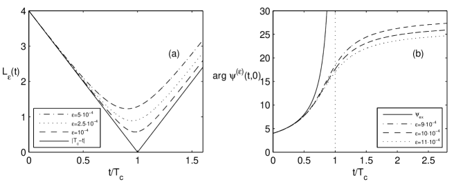
Figure 1: Solution of (16). (a): $L_{\varepsilon}(t)$ for $\varepsilon=5\cdot 10^{-4},2.5\cdot 10^{-4}$ and $10^{-4}$. Solid line is $L=|T_{c}-t|$. (b): Accumulated phase at $x=0$ for $\varepsilon=0.9\cdot 10^{-3},10^{-3}$, and $1.1\cdot 10^{-3}$. Solid line is ${\it\arg}(\psi_{\rm explicit}(t,0))$.

In order to observe the loss of the phase after the singularity, we compute the effect of small changes in the initial condition on the phase, by solving equation (16) with $\varepsilon=0.9\cdot 10^{-3},10^{-3}$ and $1.1\cdot 10^{-3}$. Figure 1(b) shows that these $\mathcal{O}(10^{-4})$ changes in the initial condition lead to $\mathcal{O}(1)$ changes in the phase for $t>T_{c}$, which is a manifestation of the post-collapse phase loss as $\varepsilon\rightarrow 0+$.

4 Sub-threshold power continuation

The main weakness of Theorem 5 is that it only applies to the explicit solutions $\psi_{\rm explicit,\alpha}$. We now generalize Merle’s continuation to generic initial profile $F({\bf x})\in H^{1}$, as follows. Consider the solution $\psi(t,{\bf x};K)$ of the critical NLS (5) with the initial condition

$$\psi_{0}({\bf x};K)=K\cdot F({\bf x}),\qquad F({\bf x})\in H^{1},\qquad K>0.$$ (18)

Let

$$K_{th}=\inf\{K~{}|~{}\psi(t,{\bf x};K)\ \mbox{collapses at some~{}$0<T_{c}(K)<\infty$}\}.$$ (19)

Let us consider the case where the infimum is attained, i.e., when $\psi(t;{\bf x};K_{th})$ becomes singular at a finite time. By construction, the solution $\psi^{(\varepsilon)}$ of the critical NLS (5) with the initial condition

$$\psi_{0}^{(\varepsilon)}({\bf x})=(1-\varepsilon)\cdot\psi_{0}^{(F)}({\bf x}),\qquad\psi_{0}^{(F)}({\bf x})=K_{th}\cdot F({\bf x}),$$ (20)

exists globally for $0<\varepsilon\ll 1$, but collapses for $-1\ll\varepsilon<0$. Therefore, as in Theorem 5, we can define the continuation of $\psi(t,{\bf x};K_{th})$ beyond the singularity, by considering the limit of $\psi^{(\varepsilon)}$ as $\varepsilon\rightarrow 0+$. Using asymptotic analysis, in Section 4.2 we derive the following result, which is the non-rigorous asymptotic analog of Theorem 5:

Continuation Result 1.

Let $\psi^{(\varepsilon)}(t,r)$ be the solution of the critical NLS (5) with the initial condition (20), where $F(r)$ is radial. Assume that $\psi^{(\varepsilon=0)}(t,r)$ becomes singular at $0<T_{c}<\infty$. Then, for any $\theta\in\mathbb{R}$, there exists a sequence $\varepsilon_{n}\rightarrow 0+$ (depending on $\theta$) and a function $\phi\in L^{2}$, such that

$$\begin{array}[]{l l}\lim_{t\rightarrow T_{c}-}\left[\lim_{\varepsilon\rightarrow 0+}\psi^{(\varepsilon)}(t,r)-\psi_{\rm explicit,\alpha}(t,r)e^{i\theta_{0}}\right]=\phi(r)&\\ \quad=\lim_{t\rightarrow T_{c}+}\left[\lim_{\varepsilon_{n}\rightarrow 0+}\psi^{(\varepsilon_{n})}(t,r)-\psi_{\rm explicit,\alpha}^{*}(2T_{c}-t,r)e^{i\theta}\right],\end{array}$$ (21)

where the above limits are in $L^{2}$, $\psi_{\rm explicit,\alpha}$ is given by (8), $T_{c}$, $\alpha\in\mathbb{R}^{+}$ and $\theta_{0}\in\mathbb{R}$. Therefore, locally near the singularity, the limiting solution satisfies Properties 1 and 2.

In particular, the limiting width of the collapsing core is given by

$$L^{(0)}(t):=\lim_{\varepsilon\rightarrow 0+}L(t;\varepsilon)\sim\alpha|t-T_{c}|,\qquad t\rightarrow T_{c}\pm.$$ (22)

By Theorem 2, if $\psi(t;{\bf x};K_{th})$ is a singular solution which is not given by (10), then $||\psi(t;{\bf x};K_{th})||_{2}^{2}>P_{\rm cr}$. In that case,

$$||\phi||_{2}^{2}=\lim_{\varepsilon\rightarrow 0+}||\psi^{(\varepsilon)}||_{2}^{2}-P_{\rm cr}=||\psi(t;{\bf x};K_{th})||_{2}^{2}-P_{\rm cr}>0.$$

Corollary 1.

If

$$\psi_{0}^{(F)}({\bf x})\not=\frac{1}{\alpha T_{c}}R^{(0)}\left(\frac{|{\bf x}-{\bf x}_{0}|}{\alpha T_{c}}\right)e^{i\theta-i\frac{|{\bf x}-{\bf x}_{0}|^{2}}{4T_{c}}+i\frac{{\bf c}\cdot({\bf x}-{\bf x}_{0})}{2}},$$

the limiting solution in Continuation Result 1 is a Bourgain-Wang solution $\psi_{\rm BW}$, both before and after the singularity.

4.1 Simulations

In order to illustrate the results of Continuation Result 1, we solve numerically the one-dimensional critical NLS (16a) with the initial condition

$$\psi_{0}^{(\varepsilon)}(x)=(1-\varepsilon)\cdot\psi_{0}^{(F)}(x),\qquad\psi_{0}^{(F)}(x)=K_{th}e^{-x^{2}}.$$ (23)

We first compute the value of $K_{th}$. We solve the NLS (16a) with the initial condition $\psi_{0}=Ke^{-x^{2}}$. Figure 2(a) shows that for $K=1.48140$ the beam collapses, while for $K=1.48139$ the collapse is arrested. Therefore, $K_{th}=1.481395\pm 5\cdot 10^{-6}$.

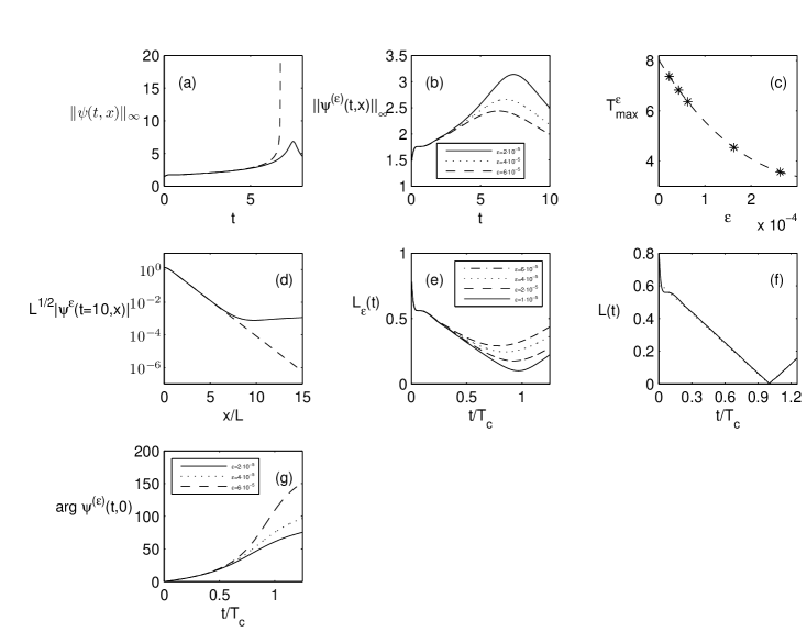
Figure 2: Solution of the one-dimensional critical NLS (16a) with: (a) The initial condition (18) with $K=1.48139$ (solid) and $K=1.48140$ (dashes). (b)–(g) the initial condition (23) with $K_{th}=1.481395$ with various values of $\varepsilon$. (b) Solution for $\varepsilon=2\cdot 10^{-5},4\cdot 10^{-5}$, and $6\cdot 10^{-5}$. (c) The maximum focusing time $T_{max}^{\varepsilon}$. (d) Rescaled solution for $\varepsilon=2\cdot 10^{-5}$ at $t=10\approx 1.35T_{max}^{\varepsilon}$ (solid), and the $R(x)$ profile (dashes), on a semi-logarithmic scale. (e) $L_{\varepsilon}(t)$ for $\varepsilon=6\cdot 10^{-5},4\cdot 10^{-5},2\cdot 10^{-5}$ and $1\cdot 10^{-5}$. (f) Extrapolation of $\{L_{\varepsilon}(t)\}$ from (e) to $\varepsilon=0$ (solid). Dashed line is $L=\alpha|T_{c}-t|$ with $\alpha=0.0777$ and $T_{c}=7.96$. (g) Accumulated phase at $x=0$.

In Figure 2(b) we plot the solution of (16a) with the initial condition (23), as a function of $t$. The solution amplitude increases up to $t=T_{max}^{\varepsilon}:=\operatorname*{arg\,max}_{t}\|\psi^{(\varepsilon)}(t,x=0)\|_{\infty}$, and then decreases. As expected, both $T_{max}^{\varepsilon}$ and the maximal amplitude $|\psi^{(\varepsilon)}(T^{\varepsilon}_{max},0)|$ increase as $\varepsilon\rightarrow 0+$. In Figure 2(c) we plot $T_{max}^{\varepsilon}$ as a function of $\varepsilon$. Extrapolation of these values to $\varepsilon=0$ shows that

$$T_{c}:=\lim_{\varepsilon\rightarrow 0+}T_{max}^{\varepsilon}\approx 8.00.$$ (24)

Since $T_{c}<\infty$, $\psi(t,x;K_{th})$ is a singular solution.

In order to confirm that the profile of the collapsing core is a rescaled $R^{(0)}$ profile, see equation (21), in Figure 2(d) we plot $|\psi^{(\varepsilon)}|$ for $\varepsilon=2\cdot 10^{-5}$ at  $t=10\approx 1.35T_{max}^{\varepsilon}$, i.e., after it collapse has been arrested, and observe that for $0\leq x/L(t)\leq 5$, the rescaled profile is indistinguishable from $R^{(0)}$, while for $6<x/L(t)$ the two curves are different. This confirms that the inner core collapses with the $\psi_{\rm explicit,\alpha}$ profile, but the outer tail does not.

In Figure 2(e) we plot the solution width $L_{\varepsilon}(t)$ for various values of $\varepsilon$. The extrapolation of these curves to $\varepsilon=0$ is in good agreement with the predicted linear limit (22) for $0.25\leq t/T_{c}\leq 1.2$, see Figure 2(f). Finally, in order to observe the loss of the phase after the singularity, we compute the effect of $\mathcal{O}(10^{-5})$ changes in the initial condition on the phase, by solving the one-dimensional NLS (16a) with the initial condition (23) with $\varepsilon=2\cdot 10^{-5},4\cdot 10^{-5}$ and $6\cdot 10^{-5}$. Figure 2(g) shows that these $\mathcal{O}(10^{-5})$ changes in the initial condition lead to $\mathcal{O}(1)$ changes in the phase for $8\leq t\leq 10$. Since  $T_{c}\approx 8$, see (24), these $\mathcal{O}(1)$ changes occur after the singularity, in agreement with Continuation Result 1.

4.2 Proof of Continuation Result 1

4.2.1 Adiabatic collapse - review

In order to compute asymptotically the limit of $\psi^{\varepsilon}$ as $\varepsilon\rightarrow 0+$, we recall that, in general, the collapse of radial solutions with power close to $P_{\rm cr}$ can be divided into two stages, see [9]:

1. During the initial non-adiabatic self-focusing stage, the solution ”splits” into a collapsing core $\psi_{\rm core}$ and a non-collapsing ”tail”, i.e.,

   $$\psi(t,r)\sim\left\{\begin{array}[]{l l}\psi_{\rm core}&\quad 0\leq\frac{r}{L(t)}\leq\rho_{0},\\ \psi_{\rm tail}&\quad\quad\rho_{0}\ll\frac{r}{L(t)},\end{array}\right.$$ (25a)

   where $$L(t) \rho_{0}=\mathcal{O}(1)$$ is the collapsing core ”width” and .

2. As $t\rightarrow T_{c}$, $\psi_{\rm core}$ approaches the self-similar profile

   $$\psi_{R^{(0)}}=\frac{1}{L^{d/2}(t)}R^{(0)}(\rho)e^{iS},\quad\rho=\frac{r}{L},\quad S=\tau(t)+\frac{L_{t}}{L}\frac{r^{2}}{4},\quad\tau=\int_{0}^{t}\frac{1}{L^{2}(s)}ds,$$ (25b)

   where $R^{(0)}$ is the ground state of (6). In contrast, the ”tail” continues to propagate forward. In particular, $\lim_{t\rightarrow T_{c}}\psi_{\rm tail}=\phi({\bf x})\in L^{2}$, see Theorem 3.

   Once the profile of $\psi_{\rm core}$ is close enough to $\psi_{R^{(0)}}$, the dynamics of the collapsing core becomes nearly adiabatic, and is governed, to leading order, by the reduced equations [20, 21, 22]

   $$\beta_{t}(t)=-\frac{\upsilon(\beta)}{L^{2}},\qquad L_{tt}=-\frac{\beta}{L^{3}},$$ (26)

   where

   $$\upsilon(\beta)=\left\{\begin{array}[]{l l}c_{\nu}e^{-\pi/\sqrt{\beta}},&\qquad\beta>0,\\ 0,&\qquad\beta\leq 0,\\ \end{array}\right.$$ (27a)

   and

   $$c_{\nu}=\frac{2A^{2}_{R}}{M},\quad A_{R}=\lim_{r\rightarrow\infty}e^{r}r^{(d-1)/2}R^{(0)}(r),\quad M=\frac{1}{4}\int_{0}^{\infty}r^{2}(R^{(0)})^{2}r^{d-1}dr.$$ (27b)

   In addition, the parameter $\beta$ is proportional to the excess power above $P_{\rm cr}$ of the collapsing core $\psi_{\rm core}$, i.e.,

   $$\beta\sim\frac{\|\psi_{\rm core}\|_{2}^{2}-P_{\rm cr}}{M},$$ (28)

   see [8, 9].

4.2.2 Asymptotic analysis

For simplicity, we assume that the initial condition (20) is radial. By construction, for the initial condition (20),

$$\left\{\begin{array}[]{l l}\|\psi_{\rm core}\|_{2}^{2}>P_{\rm cr}&\quad\varepsilon<0,\\ \|\psi_{\rm core}\|_{2}^{2}<P_{\rm cr}&\quad\varepsilon>0.\\ \end{array}\right.$$

Therefore, by (28),

$$\left\{\begin{array}[]{l l}\beta>0&\quad\varepsilon<0,\\ \beta<0&\quad\varepsilon>0.\\ \end{array}\right.$$ (29)

Hence, by (27a), $\upsilon(\beta)\equiv 0$ for $\varepsilon>0$. Therefore $\beta_{t}(t;\varepsilon)\equiv 0$. Thus, the self-focusing dynamics is governed by

$$L_{tt}(t;\varepsilon)=-\frac{\beta(\varepsilon)}{L^{3}},$$ (30)

where $\beta(\varepsilon)$ is independent of $t$.

Let $t_{ad}(\varepsilon)>0$ denote the time at which $\psi^{(\varepsilon)}$ ”enters” the adiabatic stage, i.e., when $\psi^{(\varepsilon)}\sim\psi_{R^{(0)}}$, so that equations (26) hold. Therefore, for $t\geq t_{ad}(\varepsilon)$, the dynamics is given by

$$L_{tt}(t)=-\frac{\beta(\varepsilon)}{L^{3}},\qquad L(t_{ad})=L_{ad}(\varepsilon),\quad L_{t}(t_{ad})=L^{\prime}_{ad}(\varepsilon).$$ (31)

Lemma 1.

Let $L(t;\varepsilon)$ be the solution of (31). Denote

$$t_{ad}:=\lim_{\varepsilon\rightarrow 0+}t_{ad}(\varepsilon),\qquad\alpha:=\lim_{\varepsilon\rightarrow 0+}L_{t}(t_{ad}(\varepsilon);\varepsilon),\qquad T_{c}:=\lim_{\varepsilon\rightarrow 0+}\left(-\frac{L_{ad}(\varepsilon)L^{\prime}_{ad}(\varepsilon)}{(L^{\prime}_{ad}(\varepsilon))^{2}-\frac{\beta(\varepsilon)}{L_{ad}^{2}(\varepsilon)}}\right).$$ (32)

Then,

$$\lim_{\varepsilon\rightarrow 0+}L(t;\varepsilon)=\alpha|t-T_{c}|,\qquad t_{ad}\leq t<\infty.$$ (33)

Proof.     Two integrations show that the solution of (31) is given by

$$L^{2}(t;\varepsilon)=c_{1}(\varepsilon)\left(t+\frac{L_{ad}(\varepsilon)L^{\prime}_{ad}(\varepsilon)}{c_{1}(\varepsilon)}\right)^{2}-\frac{\beta(\varepsilon)}{c_{1}(\varepsilon)},\qquad c_{1}(\varepsilon)=(L^{\prime}_{ad}(\varepsilon))^{2}-\frac{\beta(\varepsilon)}{L_{ad}^{2}(\varepsilon)}.$$

By (29), $\lim_{\varepsilon\rightarrow 0+}\beta(\varepsilon)=0$. Therefore, $\lim_{\varepsilon\rightarrow 0+}c_{1}(\varepsilon)=\alpha^{2}$. Hence, $\lim_{\varepsilon\rightarrow 0+}L^{2}(t;\varepsilon)=\alpha^{2}(t-T_{c})^{2}$. $\Box$

Corollary 2.

$\lim_{\varepsilon\rightarrow 0+}\tau(t=T_{c};\varepsilon)=\infty$.

Proof.     By (25b) and (33),

$$\lim_{\varepsilon\rightarrow 0+}\tau(t=T_{c};\varepsilon)=\lim_{\varepsilon\rightarrow 0+}\int_{0}^{T_{c}}\frac{dt}{L^{2}(t;\varepsilon)}=\int_{0}^{T_{c}}\frac{dt}{\alpha^{2}(T_{c}-t)^{2}}=\infty.$$

$\Box$

In order to go back from $L(t)$ to $\psi$, let us note that:

Lemma 2.

Let $\psi_{R^{(0)}}$ be given by (25b). If $L(t)=\alpha|T_{c}-t|$, then

$$\psi_{R^{(0)}}(t,r)=\left\{\begin{array}[]{l l}e^{i\theta_{0}}\psi_{\rm explicit,\alpha}(t,r),&\qquad 0\leq t<T_{c},\\ e^{i\theta_{1}}\psi_{\rm explicit,\alpha}^{*}(2T_{c}-t,r),&\qquad t>T_{c},\end{array}\right.$$ (34)

where $\psi_{\rm explicit,\alpha}(t,r)$ is given by (8), and $\theta_{0},\theta_{1}\in{\mathbb{R}}$.

4.2.3 Proof of Continuation Result 1

In Lemma 1 we saw that the solution $L(t)$ of the reduced system is given by (33) for $t_{ad}\leq t<\infty$. Therefore, by Lemma 2, when $t_{ad}\leq t<T_{c}$, $\psi_{R^{(0)}}(t,r)=\psi_{\rm explicit,\alpha}(t,r)e^{i\theta_{0}}$, and when $T_{c}<t$, $\psi_{R^{(0)}}(t,r)=\psi_{\rm explicit,\alpha}^{\ast}(2T_{c}-t,r)\lim_{\epsilon_{n}\to 0}e^{i\theta_{1}(\epsilon_{n})}$.

Since $\arg\psi(t,0)\sim\arg\psi_{R^{(0)}}(t,0)=\tau(t)$, Corollary 2 shows that the limiting phase becomes infinite at $T_{c}$, hence also for $t>T_{c}$. Therefore, for a given $t>T_{c}$ and $\theta\in\mathbb{R}$, there exists a sequence $\varepsilon_{n}\rightarrow 0+$, such that $\lim_{\varepsilon_{n}\rightarrow 0+}\arg\psi^{(\varepsilon_{n})}(t,0)=\theta$. Since as $t\rightarrow T_{c}$, $\psi_{\rm core}\rightarrow\psi_{R^{(0)}}$ and $\psi_{\rm tail}\rightarrow\phi({\bf x})\in L^{2}$, the Proposition follows.

5 Time-reversible continuations

The continuation in Continuation Result 1 preserves Properties 1 and 2 of Merle’s first continuation. We now show that these two properties hold for continuations of the NLS that preserve the NLS invariance under the transformation,

$$t\rightarrow-t\quad\mbox{and}\quad\psi\rightarrow\psi^{\ast},$$ (35)

and also satisfy some additional conditions.

Continuation Result 2.

Let $\psi(t,{\bf x})$ be a solution of the NLS (1) that blows up at $T_{c}$, and let $\psi^{(\varepsilon)}(t,{\bf x})$ be a smooth continuation of $\psi(t,{\bf x})$, such that

1. $\psi^{(\varepsilon)}$ exists globally for $0<\varepsilon\ll 1$.

2. $\lim_{\varepsilon\rightarrow 0+}\psi^{(\varepsilon)}(t,{\bf x})=\psi(t,{\bf x})$ in $L^{2\sigma+2}$ for $0\leq t<T_{c}$.

3. $\psi^{(\varepsilon)}$ is invariant under the transformation (35).

4. $\lim_{t\rightarrow T_{c}}\arg\psi(t,0)=\infty$.

5. Let $T^{\varepsilon}_{max}:=\operatorname*{arg\,max}_{t}\|\psi^{(\varepsilon)}(t,r)\|_{2\sigma+2}$ denote the time at which the collapse of $\psi^{(\varepsilon)}$ is arrested. Then, for all ${\bf x}\in{\mathbb{R}}^{d}$,

   $$\arg\psi^{(\varepsilon)}(T^{\varepsilon}_{max},{\bf x})\equiv\alpha^{(\varepsilon)},\qquad\alpha^{\varepsilon}\in\mathbb{R}.$$ (36)

Then, for any $\theta\in\mathbb{R}$, there exists a sequence $\varepsilon_{n}\rightarrow 0+$ (depending on $\theta$), such that

$$\lim_{\varepsilon_{n}\rightarrow 0+}\psi^{(\varepsilon_{n})}(T_{c}+t,{\bf x})=e^{i\theta}\psi^{\ast}(T_{c}-t,{\bf x}),\qquad t>0.$$

Hence, the continuation satisfies Properties 1 and 2.

Proof.     Assume first that $\alpha^{(\varepsilon)}=0$. Then, from the invariance of $\psi^{(\varepsilon)}$ under (35) it follows that

$$\psi^{(\varepsilon)}(T_{max}^{\varepsilon}+t,{\bf x})=\psi^{\ast(\varepsilon)}(T_{max}^{\varepsilon}-t,{\bf x}),\qquad t>0.$$ (37)

If $\alpha^{(\varepsilon)}\neq 0$, then (37) holds for $e^{-i\alpha^{(\varepsilon)}}\psi^{(\varepsilon)}$, i.e.,

$$e^{-i\alpha^{(\varepsilon)}}\psi^{(\varepsilon)}(T^{\varepsilon}_{max}+t,{\bf x})=e^{i\alpha^{(\varepsilon)}}\psi^{\ast(\varepsilon)}(T^{\varepsilon}_{max}-t,{\bf x}),\qquad t>0.$$ (38)

Hence,

$$\psi^{(\varepsilon)}(T^{\varepsilon}_{max}+t,{\bf x})=e^{i\theta^{(\varepsilon)}}\psi^{\ast(\varepsilon)}(T^{\varepsilon}_{max}-t,{\bf x}),\qquad t>0,$$ (39)

where $\theta^{(\varepsilon)}=2\alpha^{(\varepsilon)}$. Since $\lim_{\varepsilon\rightarrow 0+}\theta^{(\varepsilon)}=\lim_{\varepsilon\rightarrow 0+}\arg\psi^{(\varepsilon)}(T_{max}^{\varepsilon},0)=\infty$, there exists $\varepsilon_{n}\rightarrow 0+$ such that $\theta=\lim_{\varepsilon_{n}\rightarrow 0+}\theta^{(\varepsilon_{n})}$. In addition, from $\lim_{t\to T_{c}}||\psi(t)||_{2\sigma+2}=\infty$ and $\lim_{\epsilon\to 0}||\psi^{\epsilon}(t)||_{2\sigma+2}=||\psi(t)||_{2\sigma+2}$ for $0\leq t<T_{c}$, it follows that $\lim_{\varepsilon\rightarrow 0+}T_{max}^{\varepsilon}=T_{c}$. The result follows by taking the limit of (39). $\Box$

Continuation Result 2 holds for both the critical and the supercritical NLS. The interpretation of the conditions of Continuation Result 2 is as follows. Conditions 1 and 2 say that $\psi^{(\epsilon)}$ is a continuation of $\psi$. Condition 3 says that the continuation is time reversible. Condition 4 says that the phase of the singular solution becomes infinite at the singularity. This condition holds for all known singular solutions of the critical and supercritical NLS. Condition 5 says that at $t=T^{\varepsilon}_{max}$, the solution is collimated. Intuitively, this is because the solution is focusing for $t<T^{\varepsilon}_{max}$, and defocusing for $t>T^{\varepsilon}_{max}$.

We now confirm that the sub-threshold power continuation of Continuation Result 1 satisfies the conditions of Continuation Result 2. By (25b),

$$\psi^{(\varepsilon)}(t,r)\sim\frac{1}{L_{\varepsilon}^{d/2}(t)}R^{(0)}\left(\frac{r}{L}\right)e^{i\tau_{\varepsilon}+\frac{(L_{\varepsilon})_{t}}{L_{\varepsilon}}\frac{r^{2}}{4}},\qquad\frac{d\tau_{\varepsilon}}{dt}=\frac{1}{L_{\varepsilon}^{2}}.$$

Since $L_{\varepsilon}(t)$ attains its minimum at $T_{max}^{\varepsilon}$, then $L_{\varepsilon}^{\prime}(T_{max}^{\varepsilon})=0$. Therefore, $\arg\psi^{(\varepsilon)}(T^{\varepsilon}_{max},r)\equiv\alpha^{(\varepsilon)}$, where $\alpha^{(\varepsilon)}=\tau_{\varepsilon}(T^{\varepsilon}_{max})$. Furthermore, since $L_{\varepsilon}^{2}(t)\sim\frac{1}{\|\nabla\psi^{(\varepsilon)}\|_{2}^{2}}\sim\frac{1}{\|\nabla\psi\|_{2}^{2}}$, and since in the critical NLS $\|\nabla\psi\|_{2}^{2}\geq M(T_{c}-t)^{-1}$ [23],

$$\lim_{\varepsilon\rightarrow 0+}\tau_{\varepsilon}(T^{\varepsilon}_{max})=\lim_{\varepsilon\rightarrow 0+}\int_{0}^{T^{\varepsilon}_{max}}\frac{dt}{L_{\varepsilon}^{2}}\geq M\int_{0}^{T_{c}}\frac{dt}{T_{c}-t}=\infty.$$

Therefore, $\lim_{\varepsilon\rightarrow 0+}\alpha^{(\varepsilon)}=\infty$. Hence, $\lim_{\varepsilon\rightarrow 0+}\theta^{(\varepsilon)}=\infty$.

From all the conditions of Continuation Result 2, the only one whose validity is questionable is condition 5. It is reasonable to expect that this condition would hold for the collapsing core. There is no reason, however, why it should hold for the non-collapsing tail.

An immediate consequence of Continuation Result 2 is that

Corollary 3.

Under the conditions of Continuation Result 2, the limiting solution $\lim_{\varepsilon_{n}\rightarrow 0+}\psi^{(\varepsilon_{n})}$ is in $H^{1}$for $t>T_{c}$. Hence, the continuation leads to a point singularity, and not to a filament singularity.

In Section 6 we will see that time-reversible continuations can also lead to a filament singularity. In that case, however, condition 5 does not hold.

6 Vanishing nonlinear-saturation continuation

6.1 Merle’s second continuation

In [3], Merle presented a different continuation, which is based on arresting the collapse with an addition of nonlinear saturation.

Theorem 6.

[3] Let $d\geq 2$, and consider radial initial data $\psi_{0}(r)\in H^{1}\bigcap\{r\psi_{0}\in L^{2}\}$, such that the solution $\psi(t,{\bf x})$ of the critical NLS (5) blows up in finite time $T_{c}$. For $\varepsilon>0$ and $1+4/d<q<(d+2)/(d-2)$, let $\psi_{\varepsilon}(t,{\bf x})$ be the solution of the saturated critical NLS

$$i\psi_{t}(t,{\bf x})+\Delta\psi+|\psi|^{4/d}\psi-\varepsilon|\psi|^{q-1}\psi=0,\qquad\psi(0,{\bf x})=\psi_{0}(r).$$ (40)

If for $T_{0}>T_{c}$, there is a constant $C>0$ such that $\int|{\bf x}|^{2}|\psi_{\varepsilon}(T_{0},{\bf x})|^{2}d{\bf x}\leq C$, then:

1. There is a function $\tilde{\psi}(t,{\bf x})$ defined for $t<T_{0}$, such that for all $r_{0}>0$, $\tilde{\psi}\in\mathcal{C}([0,T_{0}),L^{2}(|{\bf x}|\geq r_{0}))$, and $\psi_{\varepsilon}(t,{\bf x})\rightarrow\tilde{\psi}(t,{\bf x})$ in $\mathcal{C}([0,T_{0}),L^{2}(|{\bf x}|\geq r_{0}))$ as $\varepsilon\rightarrow 0$.

2. For $t<T_{0}$, there is $m(t)\geq 0$ such that $|\psi_{\varepsilon}(t,{\bf x})|^{2}\rightarrow m(t)\delta({\bf x})+|\tilde{\psi}(t,{\bf x})|^{2}$ as $\varepsilon\rightarrow 0$ in the distribution sense. Furthermore,

   1. If $m(t)\neq 0$, then $\|\psi_{\varepsilon}(t,{\bf x})\|_{H^{1}}\rightarrow+\infty$ as $\varepsilon\rightarrow 0$ and $m(t)\geq P_{cr}$.

   2. If $m(t)=0$, there is a constant $c>0$ such that for all $\varepsilon$, $\|\psi_{\varepsilon}(t,{\bf x})\|_{H^{1}}<c$, and $\psi_{\varepsilon}(t,{\bf x})\rightarrow\tilde{\psi}(t,{\bf x})$ in $L^{2}$.

3. For all $t<T_{0}$, $m(t)+\int|\tilde{\psi}(t,{\bf x})|^{2}d{\bf x}=\int|\psi_{0}({\bf x})|^{2}d{\bf x}$.

Theorem 6 shows that the vanishing nonlinear saturation continuation can lead to a filament singularity. The condition $\int|{\bf x}|^{2}|\psi_{\varepsilon}(T_{0},{\bf x})\,d{\bf x}\leq C$ is believed to hold generically.

6.2 Malkin’s analysis

In [8], Malkin analyzed asymptotically the solutions of the saturated critical NLS (40) with $d=2$ and $q=5$. Malkin showed that initially, the solution follows the non-saturated NLS solution and self-focuses. Then, the collapse is arrested by the nonlinear saturation, leading to focusing-defocusing oscillations. During each oscillation, the collapsing core loses (radiates) some power. As a result, the magnitude of the oscillations decreases, so that ultimately, the solution approaches a standing-wave solution of the saturated NLS.

If we fix the initial condition $\psi_{0}$ and let $\varepsilon\longrightarrow 0+$, then as $\varepsilon$ decreases, the collapse is arrested at a later stage. For example, in Figure 3 we plot the solution of the saturated critical NLS (40) with $d=2$ and $q=5$ with the initial condition $\psi_{0}(r)=3.079e^{-r^{2}}$, and observe that as $\varepsilon$ decreases, the collapse is arrested at a later stage, and the oscillations occurs at higher amplitudes. In addition, we observe that as $t$ increases, the oscillations decreases. Hence, it is reasonable to assume that the amplitude of the limiting standing-wave increases as $\varepsilon$ decreases, and goes to infinity as $\varepsilon\longrightarrow 0+$. In addition, as $\varepsilon\longrightarrow 0+$, the power of the standing-wave of (40) approaches $P_{\rm cr}$. Therefore, Malkin’s analysis suggests that

$$m(t)\equiv P_{\rm cr},\qquad T_{c}\leq t<\infty,$$

i.e., after the singularity the limiting solution consists of a semi-infinite filament with power $P_{\rm cr}$, and a regular part with power $||\psi_{0}||_{2}^{2}-P_{\rm cr}$.

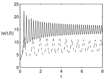
Figure 3: Solution of the saturated NLS (40) with $d=2$ and $q=5$ for $\varepsilon=0.5\cdot 10^{-3}$ (solid), and $\varepsilon=2\cdot 10^{-3}$ (dashes). Here, $\psi_{0}(r)=3.079e^{-r^{2}}$.

6.3 Importance of power radiation

The above results of Merle and Malkin strongly suggest that the continuation of singular NLS solutions with a vanishing nonlinear-saturation generically leads to a filament singularity. Since the NLS with a nonlinear saturation is time reversible, these results seem to be in contradiction with Continuation Result 2, see Corollary 3. Note, however, that in Continuation Result 2 we assumed that the solution phase is constant at the time $T_{max}^{\epsilon}$ where its collapse is arrested (Condition 5). If this condition were to hold for the solution of the saturated NLS, then by Continuation Result 2, the solution at $t=2T_{max}^{\varepsilon}$ would be given by $\psi_{0}^{*}$. As Figure 3 shows, this is not the case.

The mechanism which enables the filamentation is the loss (radiation) of power from the collapsing core to the surrounding background. Indeed, in the absence of radiation, the collapsing core of the solution of saturated NLS undergoes periodic oscillations, rather than approaches a standing wave [8]. We stress that the constant phase condition does hold asymptotically for the collapsing core [8]. It does not, however, hold for the regular part of the solution (the ”tail”).

7 Chaotic interactions

In Sections 3–5 we saw that time-reversible continuations have the property whereby the phase becomes non-unique after the blowup time. A-priori, this phase loss should have no effect, since multiplying the NLS solution by $e^{i\theta}$ does not affect the dynamics. Nevertheless, we now show that this phase loss can affect the interaction between two post-collapse beams (filaments).

Consider first the initial condition

$$\psi_{0}({\bf x})=\psi_{\rm explicit}^{tilt,\pm{\bf{c}}}(0,{\bf x}\mp{\bf x}_{0})=\psi_{\rm explicit}(0,{\bf x}\mp{\bf{x}}_{0})e^{\pm i{\bf{c}}\cdot({\bf x}\mp{\bf{x}}_{0})/2}.$$ (41)

By (9), the solution of the critical NLS (5) with the initial condition (41) is given by

$$\psi_{\rm explicit}^{tilt,\pm{\bf{c}}}(t,{\bf x}\mp{\bf x}_{0})=\psi_{\rm explicit}(t,{\bf x}\mp{\bf x}_{0}\pm{\bf{c}}\cdot t)e^{\pm i{\bf{c}}\cdot({\bf x}\mp{\bf x}_{0})/2-i|{\bf{c}}|^{2}t/4}.$$

Therefore, $\psi_{\rm explicit}^{tilt,\pm{\bf{c}}}(t,{\bf x})$ is the explicit blowup solution (7), centered initially at ${\bf x}=\pm{\bf x}_{0}$, and tilted at the angle of $\pm\arctan(|{\bf c}|)$.

We now consider the one-dimensional critical NLS (16a) with the two tilted-beams initial condition

$$\psi_{0}(x)=(1-\varepsilon)\psi_{\rm explicit}^{tilt,+c}(0,x-x_{0})+(1-(\varepsilon+\Delta\varepsilon))\psi_{\rm explicit}^{tilt,-c}(0,x+x_{0}))e^{i\Delta\theta},$$ (42)

where $\psi_{0,ex}^{tilt,\pm{\bf{c}}}$ is defined in (41) and $\varepsilon=10^{-3}$. This initial condition correspond to two input beams, centered at $\pm x_{0}$, titled toward each other, possible with a different power (when $\Delta\varepsilon\not=0$), and with a relative phase difference $\Delta\theta$. In Figure 4(a) we plot the solution when $\Delta\varepsilon=0$ and $\Delta\theta=0$ (equal-power, in-phase input beams). Since the power of each beam is slightly below $P_{\rm cr}$, each beam focuses up to a certain time ($t\approx 0.3$), and then defocuses. Subsequently, the two beams intersect around $t\approx 0.6$. Since the beams are in phase, they interact constructively. As a result, their total power is $\approx 2P_{\rm cr}$. Hence, the solution collapses at $T_{c}\approx 0.6$.

In Figure 4(b) we repeat this simulation with $\Delta\varepsilon=0$ and $\Delta\theta=\pi$ (equal-power, out-of-phase input beams). Before the two beams intersect, their dynamics is the same as in Figure 4(a). When they intersect at $t\approx 0.6$, however, the two beams are out-of-phase. Hence, they repel each other. Since each beam has power below $P_{\rm cr}$, there is no collapse.

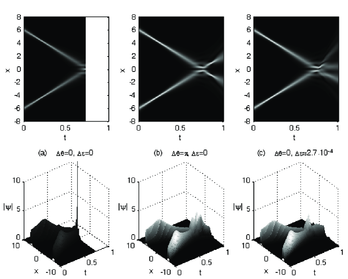
Figure 4: Solution of the one-dimensional critical NLS (16a) with the initial condition (42) with $T_{c}=0.25$, $x_{0}=6$, $c=8$ and $\varepsilon=10^{-3}$. (a): In-phase identical beams ($\Delta\theta=0$ and $\Delta\varepsilon=0$). (b): Out-of-phase identical beams ($\Delta\theta=\pi$ and $\Delta\varepsilon=0$). (c): In-phase non-identical beams  ($\Delta\theta=0$ and $\Delta\varepsilon\approx 2.7\cdot 10^{-4}$).

In Figure 4(c) we repeat this simulation with $\Delta\theta=0$ and $\Delta\varepsilon\approx 2.7\cdot 10^{-4}$ (in-phase and slightly-different input powers), and observe that at $t\approx 0.6$ the two beams repel each other and there is no collapse. In particular, comparison of Figures 4(a) and 4(c) shows that the $\mathcal{O}(10^{-4})$ change in the initial condition lead to a completely different ”post collapse” interaction pattern between the two beams.

The dynamics in Figure 4(c) is qualitatively the same as in Figure 4(b). This suggests that when the two beams in Figure 4(c) intersect, their phase difference is $\approx\pi$. Indeed, let $\psi_{1}(t,x)$ and $\psi_{2}(t,x)$ be the solutions of the one-dimensional critical NLS (16a) with the initial conditions $(1-\varepsilon)\psi_{\rm explicit}^{tilt,+c}(0,x-x_{0})$ and $(1-(\varepsilon+\Delta\varepsilon))\psi_{\rm explicit}^{tilt,-c}(0,x+x_{0}))$, respectively. In Figure 5 we plot the difference between the phases of $\psi_{1}(t,x)$ and $\psi_{2}(t,x)$, and observe that around $t\approx 0.6$, this phase difference is indeed $\approx\pi$.

We thus see that,

Conclusion 1.

Because of the loss of phase after the collapse, the phase difference between post-collapse intersecting beams becomes unpredictable.

Therefore, as noted by Merle [2], the interactions between two post-collapse beams are chaotic.

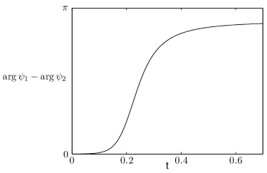
Figure 5: $\arg\psi_{1}(t,x=x_{0}-ct)-\arg\psi_{2}(t,x=-x_{0}+ct)$.

8 Ring-type singular solutions

In this section we propose a continuation of ring-type singular solutions, which is based on adding a reflecting hole with radius $r_{0}$ around the origin, and then letting $r_{0}\rightarrow 0+$.

8.1 Theory Review

Consider the two-dimensional, radially-symmetric critical NLS

$$i\psi_{t}(t,r)+\psi_{rr}+\frac{1}{r}\psi_{r}+|\psi|^{2}\psi=0,\qquad\psi(0,r)=\psi_{0}(r).$$ (43)

Let us denote the location of the maximal amplitude by

$$r_{max}(t)=\arg\max_{r}|\psi|.$$ (44)

Singular solutions of (43) are called ’peak-type’ when $r_{max}(t)\equiv 0$ for $0\leq t\leq T_{c}$, and ’ring-type’ when $r_{max}(t)>0$ for $0\leq t<T_{c}$.

Let

$$\psi_{G}^{(ex)}(t,r)=\frac{1}{L(t)}G\left(\frac{r}{L(t)}\right)e^{i\tau(t)+i\frac{L_{t}}{L}\frac{r^{2}}{4}},$$ (45a)

where

$$L(t)=\sqrt{1-\alpha^{2}t},\qquad\tau=\int_{0}^{t}\frac{1}{L^{2}(s)}ds=-\frac{1}{\alpha^{2}}\ln(1-\alpha^{2}t),$$ (45b)

and $G(\rho)$ is a solution of

$$G^{\prime\prime}(\rho)+\frac{G^{\prime}}{\rho}+\left[\frac{\alpha^{4}}{16}\rho^{2}-1\right]G+G^{3}=0,\qquad 0\neq G(0)\in\mathbb{R},\qquad G^{\prime}(0)=0.$$ (46)

In [24], Fibich, Gavish and Wang showed that $\psi_{G}^{ex}$ is an explicit ring-type solution of the radially-symmetric critical NLS (43) that blows up (in $L^{4}$) at $T_{c}=1/\alpha^{2}$. Setting $t=0$ in (45) gives the corresponding initial condition

$$\psi_{G}^{0}(r)=G(r)e^{-i(\alpha^{2}/8)r^{2}}.$$ (47)

Equation (46) has the two free parameters $\alpha$ and $G(0)$. However, in the case of a single-ring G profile, these two parameters are related [25]. For example, in the numerical simulations in this section, the G profile is the single-ring solution of (46) with

$$G(0)\approx 7.6\cdot 10^{-6},\qquad\alpha\approx 0.357832.$$ (48)

8.2 Vanishing-hole continuation

The sub-threshold power continuation approach of Section 4 cannot be applied to $\psi_{G}^{(ex)}$, since these solutions have an infinite power. In addition, this continuation cannot be applied to the ring-type singular solutions which are in $H^{1}$, since these solutions exist only for $P\gg P_{\rm cr}$ [24]. Therefore, we now develop a different continuation approach, which is based on a vanishing-hole limit.

Let $\psi(t,r)$ be a shrinking-ring singular solution of the critical NLS (43) with an initial condition $\psi_{0}(r)$. Let us add a hole around the origin with radius $r_{0}$, and impose a Dirichlet boundary condition at $r=r_{0}$, which is equivalent to placing a reflecting conductor at $r=r_{0}$. In order for the initial condition $\psi_{G}^{0}(r)$ to satisfy the Dirichlet boundary condition, we slightly modify it with a cut-off function $H_{s}(r/r_{0})$, i.e.,

$$\psi_{G}^{0}(r)\rightarrow\psi_{G}^{0,r_{0}}(r):=\psi_{G}^{0}(r)\cdot H_{s}\left(\frac{r}{r_{0}}\right).$$

We thus solve the two-dimensional, radially-symmetric critical NLS

$$i\psi_{t}(t,r)+\psi_{rr}+\frac{1}{r}\psi_{r}+|\psi|^{2}\psi=0,\qquad r_{0}<r<\infty,$$ (49a)

with the initial condition

$$\psi_{G}^{0,r_{0}}(r)\equiv G(r)e^{-i\frac{\alpha^{2}}{8}r^{2}}\cdot H_{s}\left(\frac{r}{r_{0}}\right),$$ (49b)

and the Dirichlet boundary condition

$$\psi(t,r_{0})=0,\qquad t\geq 0.$$ (49c)

A typical simulation is shown in Figure 6. Initially, the ring solution shrinks and becomes higher and narrower as it approaches the hole. After the solution is reflected outward by the hole, it expands and becomes lower and wider.

We now show that the conditions of Continuation Result 2 hold:

1. The solution of (49) exists globally, since otherwise it collapses at some $0<r_{c}<\infty$ (a standing ring), or at $r\rightarrow\infty$ (an expanding ring). The first possibility is only possible, however, if the nonlinearity is quintic or higher, and the second possibility is not possible for any power-nonlinearity, see [26].

2. By continuity, $\lim_{r_{0}\rightarrow 0+}\psi=\psi_{G}^{(ex)}$ for $0\leq t<T_{c}$.

3. The solution of (49) is invariant under the transformation (38).

4. $\lim_{t\rightarrow T_{c}}\arg\psi_{G}^{(ex)}=\infty$, see (45b).

5. Let $T_{ref}^{r_{0}}:=\arg\min_{t}{r_{max}(t)}$ denote the reflection time, where $r_{max}(t)$ is given by (44). Since the solution focuses for $0\leq t<T_{ref}^{r_{0}}$ and defocuses for $T_{ref}^{r_{0}}\leq t<\infty$, it is collimated at $t=T_{ref}^{r_{0}}$. Therefore,

   $$\arg\psi(T_{ref}^{r_{0}},r;r_{0})\equiv\alpha^{r_{0}},\qquad\alpha^{r_{0}}\in\mathbb{R}.$$ (50)

   Hence, by the arguments in the proof of Continuation Result 2,

   $$\psi(T_{ref}^{r_{0}}+t,r;r_{0})=e^{i\theta(r_{0})}\psi^{\ast}(T_{ref}^{r_{0}}-t,r;r_{0}),\qquad t>0.$$ (51)

   Indeed, in Figure 7 we plot the solution at $t=T_{ref}^{r_{0}}\pm\Delta t$ for three different values of $\Delta t$, and observe that in all three cases, the two curves lie on top of each other.

Therefore, we get the following result:

Continuation Result 3.

Let $\psi(t,r;r_{0})$ be the solution of the NLS (49), and assume that (50) holds. Then, for any $\theta\in\mathbb{R}$, there exists a sequence $r_{0,n}\rightarrow 0+$ (depending on $\theta$), such that

$$\lim_{r_{0,n}\rightarrow 0+}\psi(t,r;r_{0,n})=\left\{\begin{array}[]{l l}\psi_{G}^{(ex)}(t,r)&\qquad 0\leq t<T_{c},\\ \psi^{\ast(ex)}_{G}(2T_{c}-t,r)e^{i\theta}&\qquad T_{c}<t,\end{array}\right.$$ (52)

where $\psi_{G}^{(ex)}(t,r)$ is given by (45), and $T_{c}=1/\alpha^{2}$. Hence, this continuation satisfies Properties 1 and 2.

In particular, the limiting width is given by

$$\lim_{r_{0}\rightarrow 0+}L(t;r_{0})=\sqrt{\left|1-\frac{t}{T_{c}}\right|}.$$

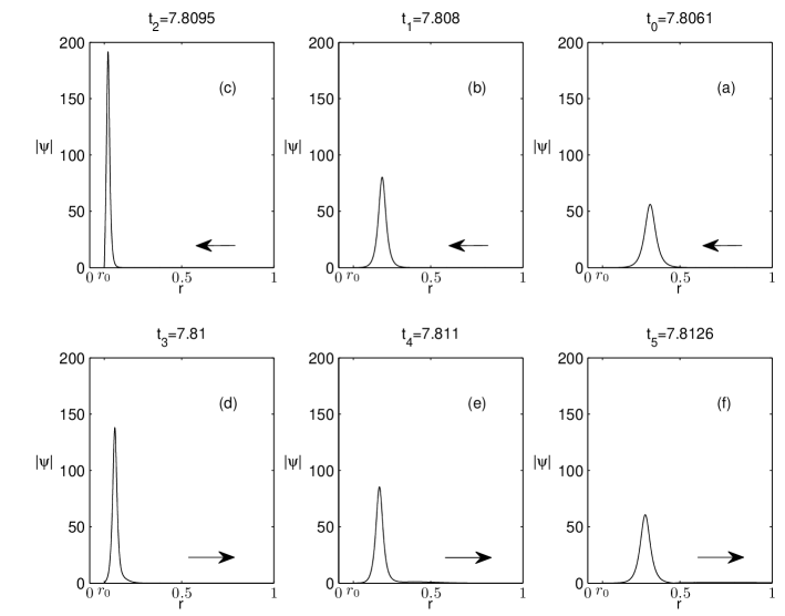
Figure 6: Solution of the NLS (49) with $r_{0}=0.08$ at (a): $t_{0}\approx 7.806$, (b): $t_{1}\approx 7.808$, (c): $t_{2}\approx 7.8095$ , (d): $t_{3}\approx 7.8100$, (e): $t_{4}\approx 7.8110$, (f): $t_{5}\approx 7.8126$. The arrows denote the direction in which the ring moves.

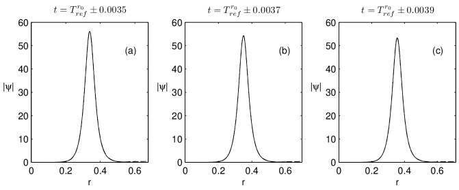
Figure 7: Solution of Figure 6 at $t=T_{ref}^{r_{0}}-\Delta t$ (solid) and at $t=T_{ref}^{r_{0}}+\Delta t$ (dashes), where $T_{ref}^{r_{0}}\approx 7.8096$. The dotted line is the best fitting $\psi_{G}$ profile. All three curves are indistinguishable.(a): $\Delta t=0.0035$. (b): $\Delta t=0.0037$. (c): $\Delta t=0.0039$.

8.2.1 Simulations

In Figure 8 we plot the reflection time as a function of $r_{0}$, and observe that this data is in excellent fit with the parabola

$$T_{ref}^{r_{0}}=\widehat{T}_{c}+k_{2}\cdot r_{0}^{2},\qquad\widehat{T}_{c}=7.80981,\qquad k_{2}=-0.03585.$$ (53)

Since $T_{c}=1/\alpha^{2}\approx 7.80983$, see (48), the extrapolation error is $\frac{\left|T_{c}-\widehat{T}_{c}\right|}{T_{c}}=0.0002\%$. The observation that $T_{c}-T_{ref}(r_{0})$ scales as $r_{0}^{2}$ and not only as $r_{0}$, will allow us to extrapolate $\psi_{G}^{r_{0}}(t,r)$ and $L(t;r_{0})$ as a function of $r_{0}^{2}$, rather than of $r_{0}$, leading to more accurate extrapolations.

We now present simulation results that support Continuation Result 3:

1. In Figure 9(a) we plot $L(t;r_{0})$ for $r_{0}=0.15,0.125,0.1$ and $0.08$. The curve which is obtained from the extrapolation of these curves to $r_{0}^{2}=0$, is nearly identical to the limiting curve $L=\sqrt{\left|1-\frac{t}{T_{c}}\right|}$, see Figure 9(b).

   

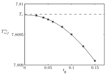
   Figure 8: The reflection time $T_{ref}^{r_{0}}$ as a function of the hole radius $r_{0}$, for the solution of the NLS (49). Solid line is the parabola (53).

   

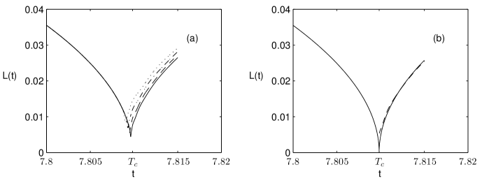
   Figure 9: Solution of the NLS (49). (a): Solution width for $r_{0}=0.15$ (dots), $r_{0}=0.125$ (dashes-dots), $r_{0}=0.1$ (dashes) and $r_{0}=0.08$ (solid). (b): Extrapolation of the curves $\{L(t;r_{0})\}$ from (a) to $r_{0}=0$ (dashes). Solid line is $L(t)=\sqrt{\left|1-t/T_{c}\right|}$.

2. In Figure 10(a) we fix the time at $t_{1}=7.8124>T_{c}$, and plot the solution profile for $r_{0}=0.15,0.125,0.1$ and $0.08$. The curve which is obtained from the extrapolation of the profiles $\{|\psi(t_{1},r;r_{0})|\}$ to $r_{0}^{2}=0$ is nearly identical to $|\psi_{G}^{\ast(ex)}(2T_{c}-t_{1},r)|$, see Figure 10(b).

   

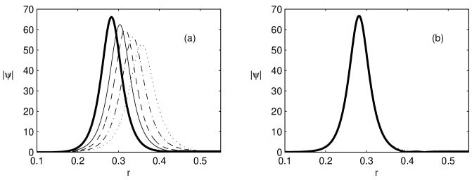
   Figure 10: (a): Solution of the NLS (49) at $t=7.8124=1.0003T_{c}$ for $r_{0}=0.15$ (dots), $r_{0}=0.125$ (dashes-dots), $r_{0}=0.1$ (dashes) and $r_{0}=0.08$ (solid). Solid bold line is the extrapolation of these curves to $r_{0}=0$. (b): The extrapolated profile from (a) (solid bold). Dotted line is $|\psi_{G}^{\ast(ex)}(2T_{c}-7.8214,r)|$. The two curves are indistinguishable.

3. In Figure 11 we plot the accumulated phase at the ring peak, i.e., $arg\,\psi_{G}^{r_{0}}(t,r_{max}(t))$, and observe that small changes in $r_{0}$ hardly affect the phase before the singularity, but lead to $\mathcal{O}(1)$ changes in the phase after the singularity.

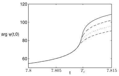
Figure 11: Accumulated phase as a function of $t$, for the solution of the NLS (49) with $r_{0}=0.08$ (solid), $r_{0}=0.1$ (dashes), $r_{0}=0.125$ (dots), and $r_{0}=0.15$ (dashes-dots).

9 Vanishing nonlinear-damping solutions

In this section, we propose a continuation which is based on the addition of nonlinear damping. The motivation for this approach comes from the vanishing-viscosity solutions of hyperbolic conservation laws. Of course, the key question is which physical mechanism should play the role of ”viscosity” in the NLS. In the nonlinear optics context, there are numerous candidates, which correspond to the mechanisms that are neglected in the derivation of the NLS from Maxwell’s equations: Nonparaxial effects, high-order nonlinearities, dispersion, plasma effects, Raman, damping, etc. Of course, for a physical mechanism to be able to play the role of ”viscosity”, it should arrest the collapse regardless of how small it is (so that we can take the limit of this term to zero, and still have global solutions). This requirement rules out some candidates (such as linear damping, see below), but still leaves plenty of potential candidates (such as nonlinear saturation, see Section 6).

In this study we consider the case when the role of viscosity is played by nonlinear damping. The addition of small nonlinear damping is ”physical”. Indeed, in nonlinear optics, experiments suggest that arrest of collapse is usually related to plasma formation, and nonlinear damping can be used as a phenomenological model for the multi-photon absorption by the plasma. In BEC, a quintic nonlinear damping term corresponds to losses from the condensate due to three-body inelastic recombinations. In [27], Bao, Jaksch and Markowich showed numerically that the arrest of collapse by the addition of a quintic nonlinear damping to the cubic three-dimensional NLS is in good agreement with experimental measurements. Nonlinear damping arises also in the context of the complex Ginzburg-Landau equation, see Section 10.

9.1 Effect of linear and nonlinear damping - review

In [28], Fibich studied asymptotically and numerically the effect of damping on blowup in the critical NLS, and showed that when the damping is linear, i.e.,

$$i\psi_{t}(t,\textbf{x})+\Delta\psi+|\psi|^{4/d}\psi+i\delta\psi=0,\qquad\psi(0,{\bf x})=\psi_{0}({\bf x}),$$ (54)

if the initial condition $\psi_{0}({\bf x})$ is such that the solution of (54) becomes singular for $\delta=0$, then the solution of (54) exists globally only if $\delta$ is above a threshold value $\delta_{c}>0$ (which depends on $\psi_{0}$). Therefore, linear damping cannot play the role of viscosity in defining weak solutions of the NLS. When, however, the damping exponent is critical or supercritical, i.e.,

$$i\psi_{t}(t,\textbf{x})+\Delta\psi+\left(1+i\delta\right)|\psi|^{4/d}\psi=0,\qquad\delta>0,$$ (55)

or

$$i\psi_{t}(t,\textbf{x})+\Delta\psi+|\psi|^{4/d}\psi+i\delta|\psi|^{p}\psi=0,\qquad\delta>0,\qquad p>4/d,$$ (56)

respectively, then regardless of how small $\delta$ is, collapse is always arrested. Therefore, Fibich suggested that nonlinear damping can ”play the role of viscosity” in defining weak NLS solutions, i.e., we can define the continuation

$$\psi:=\lim_{\delta\rightarrow 0+}\psi^{(\delta)},$$ (57)

where $\psi^{(\delta)}$ is the solution of (55) or (56).

Since the results in [28] are not rigorous, we now present the relevant rigorous results that exist in the literature. Passot, Sulem and Sulem proved that high-order nonlinear damping always prevents collapse for $d=2$. Antonelli and Sparber extended this result to $d=1$ and $d=3$:

Theorem 7.

[29, 30] The d-dimensional cubic NLS with nonlinear damping

$$i\psi_{t}(t,{\bf x})+\Delta\psi+\lambda|\psi|^{2}\psi+i\delta|\psi|^{p-1}\psi=0,\qquad\lambda\in\mathbb{R},\quad\delta>0,$$ (58)

where $\psi_{0}({\bf x})\in H^{1}(\mathbb{R}^{d})$, $3<p<\infty$ if $d=1,2$, and $3<p<5$ if $d=3$, has a unique global in-time solution.

This rigorously shows that high-order nonlinear damping can play the role of ”viscosity”. More recently, Antonelli and Sparber proved global existence for the case where the damping exponent is equal to that of the nonlinearity:

Theorem 8.

[30] Consider the cubic nonlinear NLS with a cubic nonlinear damping

$$i\psi_{t}(t,{\bf x})+\Delta\psi+(1+i\delta)|\psi|^{2}\psi=0,$$ (59)

where $\psi_{0}({\bf x})\in H^{1}(\mathbb{R}^{d}),~{}{\bf x}\psi_{0}\in L^{2}(\mathbb{R}^{d})$, and $d\leq 3$. Then, for any $\delta\geq 1$, equation (59) has a unique global in-time solution.

Unfortunately, because of the constraint $\delta\geq 1$, Theorem 8 does not show that critical nonlinear damping can play the role of viscosity. We note, however, that the asymptotic analysis and simulations of [28] strongly suggest that the solution of (55) exists globally for any $0<\delta\ll 1$.

9.2 Explicit continuation when $\psi_{0}(r)=\psi_{\rm explicit}(0,r)$

In the special case where $\psi^{(\delta)}$ is the solution of (55) with the initial condition $\psi_{\rm explicit}(t=0)$, we can calculate explicitly the vanishing nonlinear-damping limit (57):

Continuation Result 4.

Let $\psi^{(\delta)}(t,r)$ be the solution of the NLS (55) with the initial condition

$$\psi_{0}(r)=\psi_{\rm explicit}(0,r),$$ (60)

see (7). Then, for any $\theta\in\mathbb{R}$, there exists a sequence $\delta_{n}\rightarrow 0+$ (depending on $\theta$), such that

$$\lim_{\delta_{n}\rightarrow 0+}\psi^{(\delta_{n})}(t,r)=\left\{\begin{array}[]{l l}\psi_{\rm explicit}(t,r)&\quad~{}0\leq t<T_{c},\\ \psi_{\rm explicit,\kappa}^{*}(2T_{c}-t,r)e^{i\theta}&\quad T_{c}<t<\infty,\end{array}\right.$$ (61)

where $\psi_{\rm explicit,\kappa}$ is given by (8a) with $\alpha=\kappa$,

$$\kappa=\pi\left[B_{i}(0)A^{\prime}_{i}(s^{*})-A_{i}(0)B^{\prime}_{i}(s^{*})\right]\approx 1.614,$$ (62)

$A_{i}(s)$ and $B_{i}(s)$ are the Airy and Bairy functions, respectively, and $s^{*}\approx-2.6663$ is the first negative root of $G(s)=\sqrt{3}A_{i}(s)-B_{i}(s)$.

In particular, the limiting width of the solution is given by

$$\lim_{\tilde{\delta}\rightarrow 0+}L(t;\delta)=\left\{\begin{array}[]{l l}T_{c}-t&\quad 0\leq t<T_{c},\\ \kappa(t-T_{c})&\quad T_{c}<t<\infty,\end{array}\right.$$ (63)

Proof.     See section 9.4. $\Box$

Equation (61) provides a continuation of the explicit blowup solution $\psi_{\rm explicit}$ beyond the singularity. As with all the continuations that we saw so far, the weak solution is only determined up to a multiplicative phase constant $e^{i\theta}$ (Property 1). In contrast with these continuations, however, the continuation (61) is asymmetric with respect to $T_{c}$, since $\kappa\neq 1$. Therefore, it does not satisfy Property 2. This is due to the directionality in $t$ of the damping effect, i.e., the fact that equation (55) is not invariant under the transformation (35).

Remark 1.

The value of $\kappa$ is also given by, see (94),

$$\kappa=\frac{A_{i}(0)}{-A_{i}(s^{*})}.$$

Remark 2.

The limiting solution in Continuation Result 4 does not have a non-collapsing ”tail”, since the power of $\psi_{\rm explicit,\kappa}^{*}(2T_{c}-t,r)e^{i\theta}$ is equal to that of $\psi_{0}(r)$.

Remark 3.

In order to understand why $L_{t}^{2}$ increases (and not decreases) after the singularity, we note that while the vanishing nonlinear-damping does not affect the solution power, it increases the Hamiltonian, see Section 9.5. Since

$$H(\psi_{\rm explicit,\alpha})=\frac{L_{t}^{2}}{4}||rR^{(0)}||_{2}^{2}=M\alpha^{2},$$

the increase in the Hamiltonian implies that the defocusing velocity (angle) should be higher than the focusing velocity (angle), see Figure 12.

Figure 12: The vanishing nonlinear damping limit (61) for $d=1$ and $T_{c}=1$. (a) Color plot. (b) Contour plot. (c) Surface plot.

9.2.1 Simulations

In order to provide numerical support to Continuation Result 4, we solve numerically the damped NLS (55) with $d=1$ and the initial condition (60) with $T_{c}=1$, for various values of $\delta$. Figure 13(a) shows that as $\delta\rightarrow 0+$, the maximal amplitude increases, and that it is attains at $T^{\delta}_{max}\rightarrow T_{c}$. Figures 13(b) and 13(c) show that $\lim_{\delta\rightarrow 0+}L(t;\delta)$ is given by (63), and that

$$\lim_{\tilde{\delta}\rightarrow 0}L_{t}(t;\delta)=\left\{\begin{array}[]{l l}-1&\quad 0\leq t<T_{c},\\ \kappa&\quad T_{c}<t<\infty,\end{array}\right.$$ (64)

respectively, where $\kappa$ is defined in (62).

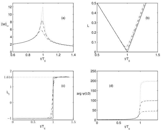
Figure 13: Solution of the damped NLS (55) with $d=1$ and the initial condition (60) with $T_{c}=1$ for $\delta=10^{-5}$ (dashes-dots), $\delta=10^{-6}$ (dashes) and $\delta=1.25\cdot 10^{-7}$ (dots). (a): $\|\psi\|_{\infty}$. (b): $L(t;\delta)$, recovered from $\psi$ using (17). Solid line is (63). (c): $L_{t}(t;\delta)$. Solid line is (64). (d): Accumulated phase at $x=0$.

In Figure 13(d) we plot the accumulated phase at $x=0$, and observe that small changes in $\delta$ have a negligible effect on the phase before the singularity, but an $\mathcal{O}(1)$ effect on the phase after the singularity, which is an indication that phase of the weak solution becomes non-unique for $t>T_{c}$.

9.3 Continuation for loglog collapse

Let $\psi$ be a solution of the undamped critical NLS that undergoes a loglog collapse. Since nonlinear damping leads to defocusing (and not to oscillations) after it arrests the collapse [28], the limiting solution has a point singularity and not a filament singularity. Indeed, the continuation has an infinite-velocity expanding core:

Continuation Result 5.

Let $\psi_{0}(r)$ be a radial initial condition, such that the corresponding solution $\psi$ of the undamped critical NLS (5) collapses with the $\psi_{R^{(0)}}$ profile at the loglog law blowup rate at $T_{c}$. Let $\psi^{(\delta)}$ be the solution of the damped NLS (55) with the same initial condition. Then,

$$\lim_{\delta\to 0+}\psi^{(\delta)}=\psi,\qquad 0\leq t<T_{c}.$$

In addition, for any $0<\delta\ll 1$, there exists $\theta(\delta)\in\mathbb{R}$, and a function $\phi\in L^{2}$, such that

$$\lim_{\delta\rightarrow 0+}\left[\psi^{(\delta)}(t,r)-{{\psi^{\ast}_{R^{(0)}}}}(2T_{c}-t,r;\delta)e^{i\theta(\delta)}\right]\stackrel{{\scriptstyle L^{2}}}{{\longrightarrow}}\phi(r),\qquad t\longrightarrow T_{c}+,$$

where $\psi_{R^{(0)}}$ is given by (25b) with some function $L(t;\delta)$, such that

$${{\lim_{t\rightarrow T_{c}+}\lim_{\delta\rightarrow 0+}L(t;\delta)=0,\qquad\lim_{t\rightarrow T_{c}+}\lim_{\delta\rightarrow 0+}L_{t}(t;\delta)=\infty}},\qquad\lim_{\delta\rightarrow 0+}\theta(\delta)=\infty.$$

Proof.     See Section 9.6. $\Box$

The post-collapse infinite velocity of the expanding core, is a consequence of the infinite velocity of the loglog collapse before the singularity, and the increase of the velocity after the singularity (see Remark 3).

Remark 4.

Because of the infinite velocity of the expanding core, it ”immediately” interacts with the non-collapsing tail. Therefore, the validity of the reduced equations that are used in the derivation of Continuation Result 5 breaks down “shortly” after the arrest of collapse. See Section 9.6.4 for further discussion.

9.3.1 Simulations

In order to illustrate Continuation Result 5 numerically, in Figures 14–15 we solve the damped NLS (55) with $\psi_{0}=\sqrt{1.05}\psi_{\rm explicit}(t=0)$ for $\delta=2\cdot 10^{-3}$, $\delta=1.5\cdot 10^{-3}$, and $\delta=10^{-3}$, and observe that the solutions are highly asymmetric with respect to $T_{max}^{(\delta)}$. In addition, as $\delta\rightarrow 0+$, the post-collapse expansion of the singular core becomes faster and faster.

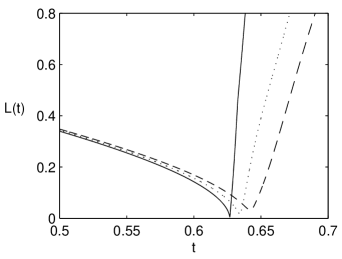
Figure 14: $L(t)$ for the solution of the damped NLS (55) with $d=1$, and the initial condition $\psi_{0}(r)=\sqrt{1.05}\psi_{\rm explicit}(t=0,r;T_{c}=1)$ for $\delta=10^{-3}$ (solid), $\delta=2\cdot 10^{-3}$ (dots), and $\delta=2.5\cdot 10^{-3}$ (dashes).

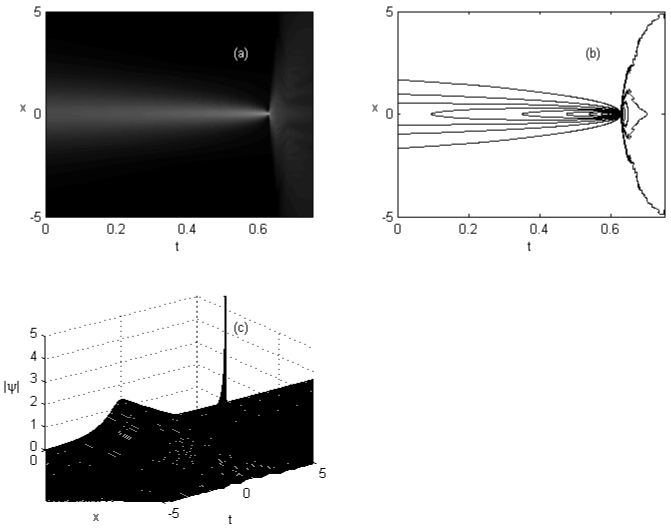
Figure 15: Same as Figure 12 for the numerical solution of the damped NLS (55) with $d=1$, $\delta=10^{-3}$, and the initial condition $\psi_{0}(r)=\sqrt{1.05}\psi_{\rm explicit}(t=0,r;T_{c}=1)$.

9.4 Proof of Continuation Result 4

In order to prove Continuation Result 4, we first approximate the NLS (55) with a reduced system of ordinary differential equations. Then, we solve the reduced system explicitly as $\delta\rightarrow 0+$.

9.4.1 Reduced equations

Lemma 3.

Let $\psi^{(\delta)}$ be the solution of the damped NLS (55) with the initial condition (60). If $\psi^{(\delta)}\sim\psi_{R^{(0)}}$, see (25), the reduced equations for $L(t)$ are given by

$$\beta_{t}(t)=-\frac{\tilde{\delta}}{L^{2}},\qquad\tilde{\delta}=\frac{2c_{d}\delta}{M},$$ (65a)

$$L_{tt}(t)=-\frac{\beta(t)}{L^{3}},$$ (65b)

where $c_{d}=\|R^{(0)}\|_{4/d+2}^{4/d+2}$, and $M$ is given by (27), with the initial conditions

$$\beta(0)=0,\qquad L(0)=T_{c},\qquad L_{t}(0)=-1.$$ (66)

Proof.     In [28], Fibich used modulation theory [9] to show that when $\psi_{\rm core}\sim\psi_{R^{(0)}}$, self focusing in (55) is given, to leading-order, by

$$\beta_{t}(t)=-\frac{\upsilon(\beta)}{L^{2}}-\frac{2c_{d}\delta}{M}\frac{1}{L^{2}},\qquad\beta(t)=-L^{3}L_{tt},$$ (67)

where $\upsilon(\beta)$ is given by (27). We recall that when $\delta=0$, the initial condition (60) leads to the explicit blowup solution (7), for which $L(t)=T_{c}-t$. Therefore, when $\delta=0$,

$$L(0)=T_{c},\qquad L_{t}(0)=-1,\qquad L_{tt}(0)=0.$$ (68)

The initial condition is independent of the subsequent dynamics, hence it is independent of $\delta$. Therefore, the initial condition is also given by (68) for $\delta>0$. Therefore, since $\beta(t)=-L^{3}L_{tt}$, then $\beta(0)=0$. Now, since $\upsilon(\beta=0)=0$, see (27), by (67) we have that $\beta_{t}<0$. Therefore, $\beta\leq 0$, and consequently $\upsilon(\beta)\equiv 0$, see (27). $\Box$

9.4.2 Simulations

The derivation of the reduced equations (65) is based on modulation theory, which is not rigorous. Therefore, we now provide numerical support for the validity of (65). In Figure 16 we solve (65) numerically for $d=1$ and various values of $\delta$. We compare these solutions with direct simulations of the damped NLS (55) with $d=1$ and the initial condition (60), from which we extract the value of $L(t)$ using (17). When $\delta=10^{-2}$, the two curves are similar, and for $\delta\leq 10^{-4}$ the two curves are indistinguishable. This confirms that as $\delta\rightarrow 0+$, the dynamics of the solution of the damped NLS (55) with the initial condition (60) is given by the reduced equations (65).

In Figure 17 we plot the rescaled profile $L^{1/2}(t)|\psi(t,x/L)|$ at $t=0.6<T_{c}$ and at $t=1.4>T_{c}$. The two rescaled profiles are indistinguishable from each other and also from $R(x)$, providing support to the assumption that $\psi^{(\delta)}\sim\psi_{R^{(0)}}$, which was used in the derivative of the reduced equations [9].

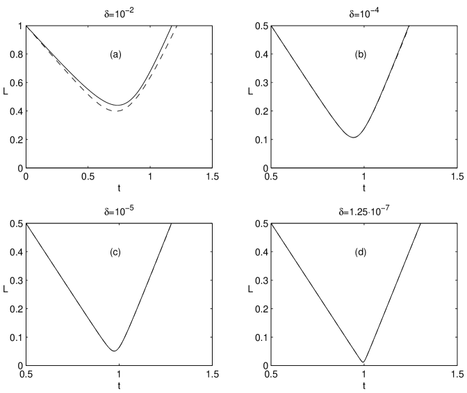
Figure 16: Width $L(t)$ of the solution of the damped NLS (55) with $d=1$ and the initial condition (60) with $T_{c}=1$ (solid). Dashed line is the solution of the reduced equations (65)-(66). (a): $\delta=10^{-2}$. (b): $\delta=10^{-4}$. (c): $\delta=10^{-5}$. (d): $\delta=1.25\cdot 10^{-7}$.

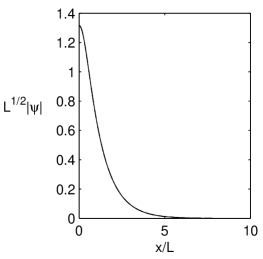
Figure 17: Rescaled profile $L^{1/2}(t)|\psi(t,x/L)|$ of the solution of the damped NLS (55) with $d=1$ and the initial condition (60) with $T_{c}=1$ and $\delta=1.25\cdot 10^{-7}$, at $t=0.6<T_{c}$ (solid) and at $t=1.4>T_{c}$ (dots), where $L(t)$ is given by (17). The dashed curve is $R(x)$. All three curves are indistinguishable.

9.4.3 Analysis of the reduced equations

Our ultimate goal is to solve the ODE system (65) with the initial conditions (66) explicitly as $\delta\rightarrow 0+$. We first prove the following Lemma:

Lemma 4.

The solution of the reduced equations (65) with the initial conditions (66) can be written as

$$L(t)=1/A(s(t)),$$

where

$$A(s)=\pi\left[\tilde{\delta}^{-1/3}A_{i}(0)-\frac{1}{T_{c}}A^{\prime}_{i}(0)\right]\left[\sqrt{3}A_{i}(s)-B_{i}(s)\right]+\frac{1}{T_{c}}\frac{B_{i}(s)}{B_{i}(0)},$$ (69)

$A_{i}(s)$ and $B_{i}(s)$ are the Airy and Bairy functions, respectively, and

$$s(t)=-\tilde{\delta}^{1/3}\int_{0}^{t}A^{2}(w)\,dw.$$ (70)

Proof.     Equation (65a) can be rewritten as

$$\beta_{\tau}=-\tilde{\delta},\qquad\tau=\int_{0}^{t}\frac{1}{L^{2}(s)}ds.$$

Since $\beta(t=0)=\beta(\tau=0)=0$,

$$\beta(\tau)=-\tilde{\delta}\tau.$$ (71)

We recall that [9]

$$\beta=\frac{A_{\tau\tau}}{A},\qquad A=\frac{1}{L}.$$ (72)

Substituting (71) in (72) gives $A_{\tau\tau}=-\tilde{\delta}\tau A$. The variable change $s=-\tilde{\delta}^{1/3}\tau$ transforms this equation into Airy’s equation

$$A_{ss}=sA.$$ (73)

Since $A=1/L$, then by (66) and (70), the initial condition for (73) are

$$A(s=0) = A(t=0)=\frac{1}{T_{c}},$$ (74a)

$$A_{s}(s=0) = -\tilde{\delta}^{-1/3}A_{t}(t=0)A^{-2}(t=0)=-\tilde{\delta}^{-1/3}.$$ (74b)

The solution of Airy’s equation is a linear combination of the Airy and Bairy functions:

$$A(s)=k_{1}A_{i}(s)+k_{2}B_{i}(s).$$ (75)

Substituting (74) in (75) gives

$$k_{1}=\frac{\tilde{\delta}^{-1/3}B_{i}(0)+\frac{1}{T_{c}}B^{\prime}_{i}(0)}{A_{i}(0)B^{\prime}_{i}(0)-A^{\prime}_{i}(0)B_{i}(0)},\quad k_{2}=-\frac{\tilde{\delta}^{-1/3}A_{i}(0)+\frac{1}{T_{c}}A^{\prime}_{i}(0)}{A_{i}(0)B^{\prime}_{i}(0)-A^{\prime}_{i}(0)B_{i}(0)}.$$

The Airy and Bairy functions satisfy the Wronskian relation

$$A_{i}(s)B^{\prime}_{i}(s)-A^{\prime}_{i}(s)B_{i}(s)=\frac{1}{\pi}.$$ (76)

Therefore,

$$k_{1}=\pi\left(\tilde{\delta}^{-1/3}B_{i}(0)+\frac{1}{T_{c}}B^{\prime}_{i}(0)\right),\quad k_{2}=-\pi\left(\tilde{\delta}^{-1/3}A_{i}(0)+\frac{1}{T_{c}}A^{\prime}_{i}(0)\right).$$ (77)

The Airy and Bairy function satisfy

$$A_{i}(0)=B_{i}(0)/\sqrt{3},\qquad A^{\prime}_{i}(0)=-B^{\prime}_{i}(0)/\sqrt{3}.$$ (78)

Substituting of (77) in (75), using relations (78) and (76) leads to (69). $\Box$

9.4.4 $\tilde{\delta}\rightarrow 0+$

Lemma 5.

Let $s^{*}_{\tilde{\delta}}$ be the first negative root of $A(s;\tilde{\delta})$, see (69). Then, $\lim_{s\rightarrow s^{*}_{\tilde{\delta}}}t(s;\delta)=\infty$.

Proof.     Inverting (70) gives

$$t(s^{*}_{\tilde{\delta}})=\tilde{\delta}^{-1/3}\int^{0}_{s^{*}_{\tilde{\delta}}}\frac{1}{A^{2}(s)}ds.$$

Let $0<\epsilon\ll 1$. Then,

$$t(s^{*}_{\tilde{\delta}})>\tilde{\delta}^{-1/3}\int^{s^{*}_{\tilde{\delta}}+\epsilon}_{s^{*}_{\tilde{\delta}}}\frac{1}{A^{2}(s)}ds.$$

By definition, $A(s^{*}_{\tilde{\delta}};\tilde{\delta})=0$. Furthermore, since $A(s;\tilde{\delta})$ is a nontrivial solution of Airy’s equation, then $A_{s}(s^{*}_{\tilde{\delta}};\tilde{\delta})\neq 0$, since otherwise from uniqueness it follows that $A(s;\tilde{\delta})\equiv 0$. Therefore, there exists $0<\varepsilon$ such that

$$A(s;\tilde{\delta})\sim(s-s^{*}_{\tilde{\delta}})A_{s}(s^{*}_{\tilde{\delta}};\tilde{\delta}),\qquad s^{*}_{\tilde{\delta}}\leq s\leq s^{*}_{\tilde{\delta}}+\varepsilon.$$ (79)

Hence,

$$\int^{s^{*}_{\tilde{\delta}}+\epsilon}_{s^{*}_{\tilde{\delta}}}\frac{1}{A^{2}(s)}ds\sim\frac{1}{A^{2}_{s}(s^{*}_{\tilde{\delta}};\tilde{\delta})}\int^{s^{*}_{\tilde{\delta}}+\epsilon}_{s^{*}_{\tilde{\delta}}}\frac{1}{(s-s^{*}_{\tilde{\delta}})^{2}}ds=\infty.$$

Therefore, $t(s^{*}_{\tilde{\delta}})=\infty$. $\Box$

By (70), $s(t)$ is monotonically decreasing from $s(t=0)=0$. Hence, the interval $0\leq t<\infty$ transforms to $0\geq s>s^{*}_{\delta}$. Since the Airy and the Bairy functions are bounded for $s\leq 0$, then $A(s;\tilde{\delta})$ is finite for $s\leq 0$, see (69). This shows that the solution of the damped NLS (55) does not collapse. Note that $A(s=s^{*}_{\tilde{\delta}})=0$ corresponds to an infinite beam width, i.e., to a complete diffraction.

Lemma 6.

Let $s^{*}=\lim_{\tilde{\delta}\rightarrow 0+}s^{*}_{\tilde{\delta}}$. Then, $s^{*}\approx-2.6663$ is the first negative root of

$$G(s)=0,\qquad G(s):=\sqrt{3}A_{i}(s)-B_{i}(s).$$ (80)

Proof.     By (69), as $\tilde{\delta}\rightarrow 0+$,

$$A(s)\sim\pi A_{i}(0)\tilde{\delta}^{-1/3}\left[\sqrt{3}A_{i}(s)-B_{i}(s)\right]=\pi A_{i}(0)\tilde{\delta}^{-1/3}G(s).$$ (81)

Therefore, $s^{*}$ satisfies (80). The value of $s^{*}$ was computed numerically, see Figure 18(a). $\Box$

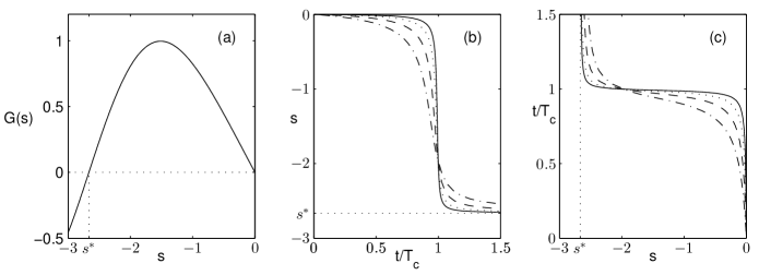
Figure 18: (a): The function $G(s)$, see (80). Here, $s^{*}$ is the first negative root of $G(s)$. (b): $s(t)$, as calculated from numerical integration of (70) for $\delta=10^{-4}$ (dashes-dots), $\delta=10^{-5}$ (dashes), $\delta=10^{-6}$ (dots) and $\delta=1.25\cdot 10^{-5}$ (solid). (c): Same as (b) for the inverse function $t(s)$.

In Figure 18(b) we plot $s(t)$ by numerically integrating (70), where A(s) is given by (69), and observe that as $\tilde{\delta}\rightarrow 0+$,  $s(t)$ tends to the step function

$$\lim_{\tilde{\delta}\rightarrow 0+}s(t)=\left\{\begin{array}[]{l l}0&\quad 0\leq t<T_{c},\\ s^{*}&\quad T_{c}<t<\infty.\end{array}\right.$$

Therefore, the inverse function $t(s)$ tends to the step function,

$$\lim_{\tilde{\delta}\rightarrow 0+}t(s)=\left\{\begin{array}[]{l l}\infty&\quad s=s^{*},\\ T_{c}&\quad s^{*}<s<0,\\ 0&\quad s=0,\end{array}\right.$$

see Figure 18(c). We now prove these limits analytically.

Lemma 7.

For any $s_{1}$ such that $-1\ll s_{1}<0$, $\lim_{\tilde{\delta}\rightarrow 0+}t(s_{1})=T_{c}$.

Proof.     Equation (69) can be rewritten as

$$A(s;\tilde{\delta})=R(s)\tilde{\delta}^{-1/3}+\frac{1}{T_{c}}F(s),$$

where

$$R(s)=\pi A_{i}(0)G(s),\qquad F(s)=\frac{B_{i}(s)}{B_{i}(0)}-\pi A^{\prime}_{i}(0)G(s).$$ (82)

Therefore,

$$t(s_{1})=\tilde{\delta}^{-1/3}\int_{s_{1}}^{0}\frac{1}{A^{2}(s)}ds=\int_{s_{1}}^{0}\frac{\tilde{\delta}^{1/3}}{\left[R(s)+\frac{\tilde{\delta}^{1/3}}{T_{c}}F(s)\right]^{2}}ds.$$ (83)

By (78), (80) and (82),

$$R(0)=0,\qquad F(0)=1,$$ (84)

and

$$R^{\prime}(0)=\pi A_{i}(0)\left(\sqrt{3}A^{\prime}_{i}(0)-B^{\prime}_{i}(0)\right)=-2\pi A_{i}(0)B^{\prime}_{i}(0).$$ (85)

Furthermore, by (78),

$$A_{i}(0)B^{\prime}_{i}(0)+A^{\prime}_{i}(0)B_{i}(0)=0,$$ (86a)

and by the Wronskian relation (76),

$$A_{i}(0)B^{\prime}_{i}(0)-A^{\prime}_{i}(0)B_{i}(0)=\frac{1}{\pi}.$$ (86b)

Adding (86a) to (86b), gives $2\pi A_{i}(0)B^{\prime}_{i}(0)=1$. Therefore, by (85),

$$R^{\prime}(0)=-1.$$ (87)

Thus, by (84) and (87),

$$R(s)\sim-s,\qquad F(s)\sim 1,\qquad-1\ll s\leq 0.$$

Substituting this in (83) gives

$$t(s_{1})\sim\int_{s_{1}}^{0}\frac{\tilde{\delta}^{1/3}}{\left[-s+\frac{\tilde{\delta}^{1/3}}{T_{c}}\right]^{2}}ds=\left[T_{c}-\frac{\tilde{\delta}^{1/3}}{-s_{1}+\frac{\tilde{\delta}^{1/3}}{T_{c}}}\right].$$ (88)

Therefore, $\lim_{\tilde{\delta}\rightarrow 0+}t(s_{1})=T_{c}$. $\Box$

From (88) it follows that

$$\lim_{\tilde{\delta}\rightarrow 0+}t(s=-c\tilde{\delta}^{1/3})=T_{c}-\frac{1}{c+\frac{1}{T_{c}}}=\frac{T_{c}}{1+\frac{1}{c}\frac{1}{T_{c}}}.$$

Therefore, $t(s)$ has a boundary layer at $s=0$ with thickness $\tilde{\delta}^{1/3}$, in which it increases monotonically from 0 to $T_{c}$. Hence,

Corollary 4.

$\lim_{\tilde{\delta}\rightarrow 0+}s(t;\tilde{\delta})=0,\qquad 0\leq t<T_{c}$.

Lemma 8.

For any $s^{*}<s_{2}<s_{1}<0$, $\lim_{\tilde{\delta}\rightarrow 0}\left(t(s_{2})-t(s_{1})\right)=0$.

Proof.     By (83),

$$t(s_{2})-t(s_{1})=\int_{s_{2}}^{s_{1}}\frac{\tilde{\delta}^{1/3}}{\left[R(s)+\frac{\tilde{\delta}^{1/3}}{T_{c}}F(s)\right]^{2}}ds.$$

Since $R(s)=\pi A_{i}(0)G(s)$ and $G(s)>0$ in $(s^{*},0)$, then $R(s)\geq c>0$ for any $s^{*}<s_{2}\leq s\leq s_{1}<0$, where $c$ is independent of $\tilde{\delta}$. Therefore, as $\tilde{\delta}\rightarrow 0+$,

$$\lim_{\tilde{\delta}\rightarrow 0}(t(s_{2})-t(s_{1}))\sim\lim_{\tilde{\delta}\rightarrow 0}\tilde{\delta}^{1/3}\int_{s_{2}}^{s_{1}}\frac{1}{R^{2}(s)}ds=0.$$

$\Box$

From Lemma 7 and Lemma 8 it follows that

Corollary 5.

$$\lim_{\tilde{\delta}\rightarrow 0}t(s)=T_{c},\qquad s^{*}<s<0.$$

Lemma 9.

$\lim_{\tilde{\delta}\rightarrow 0+}s(t;\tilde{\delta})=s^{*}$ for $T_{c}<t<\infty$.

Proof.     Since $s(t;\tilde{\delta})$ is monotonically decreasing (see equation (70)), $t(s;\tilde{\delta})\approx T_{c}$ for $s^{*}_{\tilde{\delta}}<s<0$ (Corollary 5), and $\lim_{s\rightarrow s^{*}_{\tilde{\delta}}}t(s;\tilde{\delta})=\infty$ (Lemma 5), then near $s^{*}_{\tilde{\delta}}$ there is a boundary layer in which $t$ changes from $T_{c}$ to $\infty$. Therefore, the values $(T_{c},\infty)$ are attained in the boundary layer around $s^{*}_{\tilde{\delta}}$. Since $\lim_{\tilde{\delta}\rightarrow 0+}s^{*}_{\tilde{\delta}}=s^{*}$, the result follows. $\Box$

From Corollary 4 and Lemma 9 it follows that, see Figure 18(b),

Corollary 6.

$$\lim_{\tilde{\delta}\rightarrow 0+}s(t;{\tilde{\delta}})=\left\{\begin{array}[]{l l}0&\quad 0\leq t<T_{c},\\ s^{*}&\quad T_{c}<t<\infty.\end{array}\right.$$ (89)

Our next observation concerns $L(t)$.

Lemma 10.

$$\lim_{\tilde{\delta}\rightarrow 0+}L(t)=\left\{\begin{array}[]{l l}T_{c}-t&\quad 0\leq t<T_{c},\\ \kappa(t-T_{c})&\quad T_{c}<t<\infty,\end{array}\right.$$ (90)

where $\kappa$ is defined in equation (62).

Proof.     Using $L=A^{-1}$ and (75),

$$L_{t}=-A^{-2}A_{s}\frac{ds}{dt}=-A^{-2}A_{s}(-\tilde{\delta}^{1/3}A^{2})=\tilde{\delta}^{1/3}A_{s}=\tilde{\delta}^{1/3}\left[k_{1}A^{\prime}_{i}(s)+k_{2}B^{\prime}_{i}(s)\right].$$ (91)

By (77),

$$\lim_{\tilde{\delta}\rightarrow 0+}\tilde{\delta}^{1/3}k_{1}=\pi B_{i}(0),\qquad\lim_{\tilde{\delta}\rightarrow 0+}\tilde{\delta}^{1/3}k_{2}=-\pi A_{i}(0).$$

Therefore,

$$\lim_{\tilde{\delta}\rightarrow 0}L_{t}(t)=\pi\left[B_{i}(0)A^{\prime}_{i}(\tilde{s}(t))-A_{i}(0)B^{\prime}_{i}(\tilde{s}(t))\right],\qquad\tilde{s}(t)=\lim_{\tilde{\delta}\rightarrow 0}s(t;\tilde{\delta}).$$

Hence, by (89),

$$\lim_{\tilde{\delta}\rightarrow 0}L_{t}(t)=\left\{\begin{array}[]{l l}\pi\left[B_{i}(0)A^{\prime}_{i}(0)-A_{i}(0)B^{\prime}_{i}(0)\right]&\quad 0\leq t<T_{c},\\ \pi\left[B_{i}(0)A^{\prime}_{i}(s^{*})-A_{i}(0)B^{\prime}_{i}(s^{*})\right]&\quad T_{c}<t<\infty.\end{array}\right.$$

Since $\pi\left[B_{i}(0)A^{\prime}_{i}(0)-A_{i}(0)B^{\prime}_{i}(0)\right]=-1$, see equation (76),

$$\lim_{\tilde{\delta}\rightarrow 0}L_{t}(t)=\left\{\begin{array}[]{l l}-1&\quad 0\leq t<T_{c},\\ \kappa&\quad T_{c}<t<\infty,\end{array}\right.$$

where $\kappa$ is given by (62). Since $L(0)=T_{c}$, (90) follows. $\Box$

Our last observation concerns the solution phase. By definition (25b),

$$\tau(t)=\int_{0}^{t}\frac{1}{L^{2}(s)}ds.$$

Therefore, by (90),

$$\lim_{\tilde{\delta}\rightarrow 0+}\tau(T_{c})=\int_{0}^{T_{c}}\frac{1}{(T_{c}-s)^{2}}ds=\infty.$$ (92)

Therefore, the phase information is lost at the singularity.

9.4.5 Proof of Continuation Result 4

We have that $\psi^{\delta}\sim\psi_{R^{(0)}}$, where $L(t)$ is given by (90). Therefore, by Lemma 2, when $0\leq t<T_{c}$, $\psi_{R^{(0)}}(r,t)=\psi_{\rm explicit}(t,r)$, and when $T_{c}<t$, $\psi_{R^{(0)}}(t,r)=\psi_{\rm explicit,\alpha}^{\ast}(2T_{c}-t,r)$. In addition, since $\arg\psi(t,0)\sim\arg\psi_{R^{(0)}}(t,0)=\tau(t)$, equation (92) shows that the limiting phase becomes infinite at and after the singularity. Hence, for a given given $t>T_{c}$ and $\theta\in\mathbb{R}$, there exists a sequence $\delta_{n}\rightarrow 0+$, such that $\lim_{\delta_{n}\rightarrow 0+}\arg\psi^{(\delta_{n})}(t,0)=\theta$. Hence, Continuation Result 4 follows.

9.5 Hamiltonian dynamics

In the case of a non-conservative perturbation such as nonlinear damping, the Hamiltonian of $\psi$ can be approximated with, see [9, eq. (H.5)],

$$H(\psi)\sim\frac{M}{2}(L^{2})_{tt}.$$ (93)

Since $\beta_{t}=-\frac{1}{2}L^{2}(L^{2})_{ttt}$, then

$$H_{t}\sim\frac{M}{2}(L^{2})_{ttt}=-M\frac{\beta_{t}}{L^{2}}=M\frac{\tilde{\delta}}{L^{4}}.$$

Therefore, the Hamiltonian increases with $t$. Moreover, by (70) and (81),

$$H_{s}=H_{t}\frac{dt}{ds}=M\frac{\tilde{\delta}}{L^{4}}\frac{1}{-\tilde{\delta}^{1/3}A^{2}}=-M\tilde{\delta}^{2/3}A^{2}\sim-M\pi^{2}A_{i}^{2}(0)G^{2}(s).$$

Therefore,

$$\Delta H:=H(t=\infty)-H(0)=\int_{s=0}^{s^{*}}H_{s}\,ds=M\pi^{2}A_{i}^{2}(0)\int_{s=s^{*}}^{0}G^{2}(s)\,ds.$$

Now,

$$\int_{s=s^{*}}^{0}G^{2}(s)\,ds=G^{2}s\Big{|}_{s=s^{*}}^{0}-\int_{s=s^{*}}^{0}2sGG_{s}(s)\,ds=-2\int_{s=s^{*}}^{0}sGG_{s}(s)\,ds.$$

Since $G_{ss}=sG$, then

$$\int_{s=s^{*}}^{0}G^{2}(s)\,ds=-2\int_{s=s^{*}}^{0}G_{ss}G_{s}(s)\,ds=-G_{s}^{2}\Big{|}_{s=s^{*}}^{0}.$$

Therefore,

$$\Delta H=-M\pi^{2}A_{i}^{2}(0)G_{s}^{2}\Big{|}_{s=s^{*}}^{0}.$$

Since the Wronskian of the Airy equation is a constant,

$$W(G,A)=G(s)A_{i}^{\prime}(s)-A_{i}(s)G^{\prime}(s)\equiv G(0)A_{i}^{\prime}(0)-A_{i}(0)G^{\prime}(0).$$

Therefore, since $G$ vanishes at $s=0,s^{*}$,

$$G^{\prime}(s^{*})=\frac{A_{i}(0)G^{\prime}(0)}{A_{i}(s^{*})}.$$

Also, by (87),

$$-1=R^{\prime}(0)=\pi A_{i}(0)G^{\prime}(0).$$

Therefore,

$$\Delta H=-M\pi^{2}A_{i}^{2}(0)G_{s}^{2}(0)\left(1-\left(\frac{A_{i}(0)}{A_{i}(s^{*})}\right)^{2}\right)=M\left(\left(\frac{A_{i}(0)}{A_{i}(s^{*})}\right)^{2}-1\right).$$

On the other hand, by (93), $H\sim M(L_{t}^{2}-\beta/L^{2})$. In addition, since the limiting solution has exactly the critical power, then $\lim_{\tilde{\delta}\to 0+}\beta=0$, see (28). Therefore, $\lim_{\tilde{\delta}\to 0+}H=ML_{t}^{2}$. Hence, by (64),

$$\Delta H=M(\kappa^{2}-1).$$

Comparison of the last two expressions for $\Delta H$ shows that

$$\kappa=\frac{A_{i}(0)}{|A_{i}(s^{*})|}.$$ (94)

9.6 Proof of Continuation Result 5

9.6.1 Analysis of the reduced equations

We first analyze the dynamics of the collapsing core under the assumption that it is governed by the reduced equations (67). By continuity, as $\delta\longrightarrow 0+$, the limiting solution undergoes a loglog collapse as $t\longrightarrow T_{c}-$. Therefore, as $t\longrightarrow T_{c}-$, the amount of power that collapses into the singularity is exactly $P_{\rm cr}$. Hence, by (28), $\lim_{\delta\to 0+}\beta(T_{c})=0$. Therefore, since $\beta_{t}<0$, see (67), and since $\nu(\beta)\equiv 0$ for $\beta<0$, we have that $\lim_{\delta\to 0+}\beta_{t}=0$ for $t>T_{c}$. Therefore, $\lim_{\delta\to 0+}\beta\equiv 0-$ for $t>T_{c}$. Hence, the collapsing core expands linearly with the $\psi_{R^{(0)}}$ profile. Therefore, the expanding core is given by $\psi_{\rm explicit,\alpha}^{\ast}(2T_{c}-t,r)$.

The above arguments show that according to the reduced equations, after the singularity the solution is of a Bourgain-Wang type, but do not provide the value of the expansion velocity $\alpha$. In order to do so, we now solve the reduced equations. By (67),

$$\beta_{\tau}=-\nu(\beta)-\tilde{\delta},\qquad\tau=\int_{0}^{t}\frac{1}{L^{2}(s)}ds.$$ (95)

For solutions that undergoes a loglog collapse we have that $\beta(0)>0$, see (28). For a fixed $\tilde{\delta}>0$, as $\beta\searrow 0+$, $\nu(\beta)$ becomes negligible compared with $\tilde{\delta}$. Therefore, to leading order, $\beta_{\tau}=-\tilde{\delta}$. Hence,

$$\beta(\tau)=\beta_{0}-\tilde{\delta}\tau,\qquad\beta_{0}=\beta(0)>0.$$ (96)

Substituting (96) in (72) gives $A_{\tau\tau}=(\beta_{0}-\tilde{\delta}\tau)A$. The variable change

$$s=\tilde{\delta}^{-2/3}\beta_{0}-\tilde{\delta^{1/3}}\tau$$ (97)

transforms this equation into Airy’s equation (73).

Let $A(t=0)=A_{0}=1/L_{0}$ and $A_{t}(t=0)=A_{0}^{\prime}=-L_{0}^{\prime}/(L_{0})^{2}$ be the initial conditions for $A(t)$. Therefore, the initial conditions for $A(s;\tilde{\delta})$ are

$$A(s=s_{0}) = A_{0},$$ (98a)

$$A_{s}(s=s_{0}) = -\tilde{\delta}^{-1/3}A_{t}(t=0)A^{-2}(t=0)=-\tilde{\delta}^{-1/3}\frac{A_{0}^{\prime}}{(A_{0})^{2}},$$ (98b)

where

$$s_{0}:=\tilde{\delta}^{-2/3}\beta_{0}.$$ (98c)

Therefore, $A(s;\tilde{\delta})$ is given by (75) with

$$k_{1}=\pi\left(\frac{A_{0}^{\prime}}{(A_{0})^{2}}\tilde{\delta}^{-1/3}B_{i}(s_{0})+A_{0}B_{i}^{\prime}(s_{0})\right),\quad k_{2}=-\pi\left(\frac{A_{0}^{\prime}}{(A_{0})^{2}}\tilde{\delta}^{-1/3}A_{i}(s_{0})+A_{0}A_{i}^{\prime}(s_{0})\right).$$ (99)

9.6.2 $\tilde{\delta}\rightarrow 0+$

In Figure 19(a) we plot $t(s;\tilde{\delta})$, and observe that

Lemma 11.

$$\lim_{\tilde{\delta}\rightarrow 0+}t\left(s;\tilde{\delta}\right)=\left\{\begin{array}[]{l l}0&s=s_{0},\\ T_{c}&\quad s^{\ast}<s~{}\mbox{and}~{}s_{0}-s\gg 1\\ \infty&\quad s=s^{\ast}.\\ \end{array}\right.$$ (100)

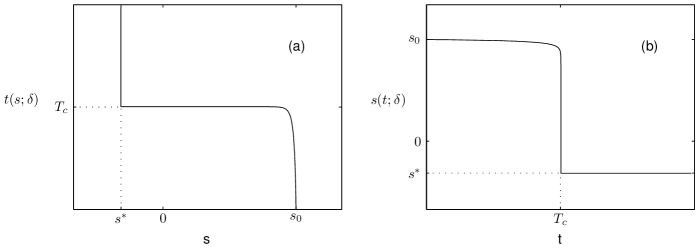
Figure 19: (a) $t(s;\delta)$. (b) $s(t;\delta)$. For  $0<\tilde{\delta}\ll 1$.

Proof.     By (95) and (97), $\frac{ds}{dt}=-\tilde{\delta}^{1/3}A^{2}$. Therefore,

$$t\left(s;\tilde{\delta}\right)=-\frac{1}{\tilde{\delta}^{1/3}}\int_{s_{0}}^{s}\frac{1}{A^{2}(s)}ds=-\frac{1}{\tilde{\delta}^{1/3}}\int_{s_{0}}^{s}\frac{1}{[k_{1}A_{i}(s)+k_{2}B_{i}(s)]^{2}}ds.$$ (101)

Following [32], it is easy to verify by direct differentiation and using the Wronskian relation (76) that

$$t\left(s;\tilde{\delta}\right)=\frac{\pi}{k_{1}\tilde{\delta}^{1/3}}\left[\frac{B_{i}(s_{0})}{A(s_{0};\tilde{\delta})}-\frac{B_{i}(s)}{A(s;\tilde{\delta})}\right]=-\frac{\pi}{k_{2}\tilde{\delta}^{1/3}}\left[\frac{A_{i}(s_{0})}{A(s_{0};\tilde{\delta})}-\frac{A_{i}(s)}{A(s;\tilde{\delta})}\right].$$ (102)

Therefore, by (98b),

$$t\left(s;\tilde{\delta}\right)=\frac{\pi}{k_{1}\tilde{\delta}^{1/3}}\left[\frac{B_{i}(s_{0})}{A_{0}}-\frac{B_{i}(s)}{A(s;\tilde{\delta})}\right]=\frac{\pi}{k_{2}\tilde{\delta}^{1/3}}\left[\frac{A_{i}(s)}{A(s;\tilde{\delta})}-\frac{A_{i}(s_{0})}{A_{0}}\right].$$ (103)

Lemma 12.

Let $s^{*}_{\tilde{\delta}}$ be the first negative root of $A(s;\tilde{\delta})$. Then, $\lim_{s\rightarrow s^{*}_{\tilde{\delta}}}t(s;\delta)=\infty$.

Proof.     This follows by direct substitution of $s^{*}_{\tilde{\delta}}$ in (103). $\Box$

Lemma 13.

Let $s^{*}:=\lim_{\tilde{\delta}\rightarrow 0+}s^{*}_{\tilde{\delta}}$. Then, $s^{\ast}\approx-2.338$ is the first (negative) root of $A_{i}(s)$.

Proof.     By (98c), $s_{0}\gg 1$ for $0<\tilde{\delta}\ll 1$. Therefore,

$$A_{i}(s_{0})\sim\frac{1}{2\sqrt{\pi}}s_{0}^{-1/4}e^{-\frac{2}{3}s_{0}^{3/2}},\qquad B_{i}(s_{0})\sim\frac{1}{\sqrt{\pi}}s_{0}^{-1/4}e^{\frac{2}{3}s_{0}^{3/2}}.$$ (104)

Hence, by (99),

$$\lim_{\tilde{\delta}\rightarrow 0+}\frac{k_{2}}{k_{1}}=0.$$ (105)

Therefore,

$$A(s;\tilde{\delta})\sim k_{1}A_{i}(s),\qquad s=\mathcal{O}(1),\quad 0<\tilde{\delta}\ll 1.$$

Thus, the result follows. $\Box$

From Lemma 12 and Lemma 13 it follows that:

Corollary 7.

$t(s^{\ast};\tilde{\delta}):=\lim_{\tilde{\delta}\rightarrow 0+}t(s^{\ast}_{\tilde{\delta}};\tilde{\delta})=\infty$.

Equation (103) can be written as

$$t\left(s;\tilde{\delta}\right)=T_{c}^{\left(\tilde{\delta}\right)}\left[1-\frac{\frac{B_{i}(s)}{B_{i}(s_{0})}}{\frac{A(s;\tilde{\delta})}{A_{0}}}\right],\qquad T_{c}^{\left(\tilde{\delta}\right)}:=\frac{\pi}{k_{1}\tilde{\delta}^{1/3}}\frac{B_{i}(s_{0})}{A_{0}}.$$ (106)

By (99) and (106),

$$T_{c}^{\left(\tilde{\delta}\right)}=\frac{\frac{\pi B_{i}(s_{0})}{k_{1}\tilde{\delta}^{1/3}A_{0}}}{\pi\left(\frac{A_{0}^{\prime}B_{i}(s_{0})}{(A_{0})^{2}\tilde{\delta}^{1/3}}+A_{0}B_{i}^{\prime}(s_{0})\right)}.$$

By (98c) and (104), $B_{i}^{\prime}(s_{0})\sim B_{i}(s_{0})\cdot s_{0}^{1/2}=B_{i}(s_{0})\cdot\delta^{-1/3}\beta_{0}^{1/2}$. Therefore, since $L=1/A$,

$$T_{c}^{\left(\tilde{\delta}\right)}\sim\frac{\frac{1}{(A_{0})^{2}}}{\frac{A_{0}^{\prime}}{(A_{0})^{3}}+\beta_{0}^{1/2}}=\frac{(L_{0})^{2}}{\beta_{0}^{1/2}-L_{0}L_{0}^{\prime}},$$

which is the adiabatic approximation of $T_{c}$, see [9, eq. (3.31)].

By (104), $B_{i}(s)/B_{i}(s_{0})$ is exponentially decreasing as $s$ decreases from $s_{0}$. Let us assume for simplicity that $A^{\prime}_{0}\geq 0$. Then, $A(s;\tilde{\delta})>A(s_{0})$. Therefore, $\frac{B_{i}(s)/B_{i}(s_{0})}{A(s;\tilde{\delta})/A_{i}(s_{0})}$ is exponentially decreasing as $s$ decreases from $s_{0}$. Hence,

$$t\left(s;\tilde{\delta}\right)\approx T_{c}^{(\tilde{\delta})}\approx T_{c},\qquad s^{\ast}<s~{}\mbox{and}~{}s_{0}-s\gg 1.$$

This concludes the proof of Lemma 11. $\Box$

From Lemma 11 it follows that

$$s(t)\sim\left\{\begin{array}[]{l l}O(s_{0})&\quad 0<t<T_{c},\\ s^{\ast}&\quad T_{c}<t,\\ \end{array}\right.\qquad as~{}\tilde{\delta}\rightarrow 0+,$$ (107)

see Figure 19(b). We recall that

$$L_{t}(t;\tilde{\delta})=\tilde{\delta}^{1/3}\left[k_{1}A_{i}^{\prime}(s(t))+k_{2}B_{i}^{\prime}(s(t))\right],$$

see (91). Hence, by (107),

$$L_{t}(t;\tilde{\delta})\sim\tilde{\delta}^{1/3}\left[k_{1}A_{i}^{\prime}(s^{\ast})+k_{2}B_{i}^{\prime}(s^{\ast})\right],\qquad T_{c}<t,\qquad~{}0<\tilde{\delta}\ll 1.$$

Therefore, by (105),

$$L_{t}(t;\tilde{\delta})\sim\tilde{\delta}^{1/3}k_{1}A_{i}^{\prime}(s^{\ast}),\qquad T_{c}<t,\quad 0<\tilde{\delta}\ll 1.$$

Hence, $L(t)$ is linear for $T_{c}<t$.

By (104) and (106),

$$k_{1}\tilde{\delta}^{1/3}\sim\frac{\pi}{A_{0}}\frac{1}{T_{c}}B_{i}(s_{0})\sim\frac{\sqrt{\pi}}{A_{0}}\frac{1}{T_{c}}s_{0}^{-1/4}e^{\frac{2}{3}s_{0}^{3/2}}.$$

Therefore,

$$L_{t}(t;\tilde{\delta})\sim\frac{\sqrt{\pi}}{A_{0}}\frac{1}{T_{c}}s_{0}^{-1/4}e^{\frac{2}{3}s_{0}^{3/2}}A_{i}^{\prime}(s^{\ast}),\qquad T_{c}<t,\qquad~{}0<\tilde{\delta}\ll 1.$$ (108)

Since $\lim_{\tilde{\delta}\rightarrow 0+}s_{0}=\infty$,

$$\lim_{\tilde{\delta}\rightarrow 0+}\tilde{\delta}^{1/3}k_{1}A^{\prime}_{i}(s^{\ast})=\infty.$$

Therefore, the post-collapse slope of $L(t)$ becomes infinite as $\tilde{\delta}\rightarrow 0+$. $\Box$

9.6.3 Simulation

In Figure 20 we solve the reduced equations (65), and observe that for $t>T_{c}$, $L_{t}(t)$ is indeed in excellent agreement with the asymptotic prediction (108).

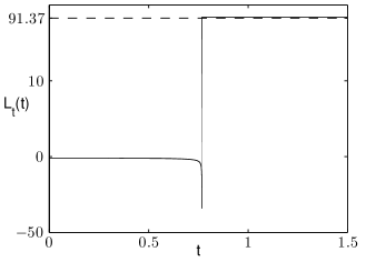
Figure 20: Solution of the reduced equations (65) with $d=1$, $\delta=2.5\cdot 10^{-4}$, and the initial conditions $L(0)=1$, $L^{\prime}_{0}=-1$, and $\beta(0)=0.1$. Solid line is $L_{t}(t)$. Dashed line is the prediction (108).

9.6.4 Validity of the reduced equations?

In the asymptotic analysis in Section 9.6 we approximated the critical NLS with the reduced equations (67). Then, we approximated the reduced equations (67) with the reduced equations (65), by neglecting $\nu(\beta)$. We now consider the validity of these approximations.

In Figure 21(a) we plot $L(t)$ for the solutions of the reduced equations (67) and (65). Although $\tilde{\delta}\approx 0.0019$ is not much larger then $\nu(\beta(0))\approx 0.0016$, the two solutions are ”close”. Plotting $L_{t}(t)$ shows that in both cases, $L_{t}(t)$ is a constant after the collapse is arrested, see Figure 21(b). The ”addition” of $\nu(\beta)$, however, decreases this constant by a factor of $\approx 4$. Therefore, when $\nu(\beta)$ is not neglected, the approximation (108) for $L_{t}(t)$ is not accurate, but the solution still expands linearly at a velocity that goes to infinity as $\delta\rightarrow 0+$.

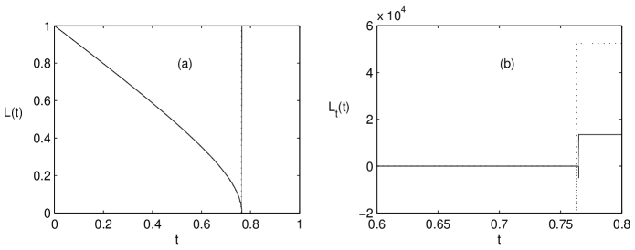
Figure 21: Solution of the reduced equations (67) [solid] and (65) [dots] with $\delta=10^{-4}$, and the initial conditions $\beta(0)=0.1$, $L_{0}=1$, and $L_{t}(0)=-1$. (a) $L(t)$. (b) $L_{t}(t)$.

In order to check the validity of the reduced equations (67) with $\nu(\beta)$, we solve the damped NLS (55) for $d=1$ with the initial condition $\sqrt{1.05}\psi_{\rm explicit}(t=0,r;T_{c}=1)$, for various values of $\delta$. Then, we extract from $\psi$ the value of $L(t)$ using (17). These NLS solutions are compared with solutions of the reduced equations (67). The initial conditions for the reduced equations are as follow. By (28), $\beta(0)\sim\frac{\|\sqrt{1.05}\psi_{explicit}\|_{2}^{2}-P_{cr}}{M}=\frac{0.05P_{cr}}{M}\approx 0.3242$. By (17), $L(0)\approx 0.9524$. For $\psi_{\rm explicit}(t=0,r;T_{c}=1)$, $L_{t}(0)=-1$, see (66). The multiplication by $\sqrt{1.05}$ leads to a small change in $L_{t}(0)$. We found that $L_{t}(0)=-1.02$ provides the best fitting.

Figure 22 shows that there is a good agreement between $L(t)$ of the reduced equations (67) and of the NLS. In addition, in both cases, the post-collapse defocusing velocity increases as $\delta$ decreases. The curves of $L_{t}(t)$ show a good agreement when the solutions focus, but differ when the solutions defocus. In particular, $L_{t}(t)$ of the NLS solution is not a constant after the arrest of collapse. We relate this difference to the interaction between the expanding core and the tail, which is ignored in the reduced equations. This core-tail interaction did not occur in the explicit continuation case, see Section 9.2, since in that case the power of the initial condition $\psi_{\rm explicit}$ is equal to $P_{cr}$, hence there is no tail. In addition, this phenomenon did not occur in the sub-threshold continuation (see Section 4), since there the expansion velocity was finite. Therefore, sufficiently close to $T_{c}+$, the expanding core had a negligible interaction with the tail.

In summary, the asymptotic analysis and numerical simulations suggest that in the nonlinear-damping continuation of NLS solutions that undergo a loglog collapse, the singular core of the NLS solution expands after the singularity with a velocity that goes to infinity as $\delta\rightarrow 0+$. The post-collapse expansion velocity is, however, probably not linear in $t$.

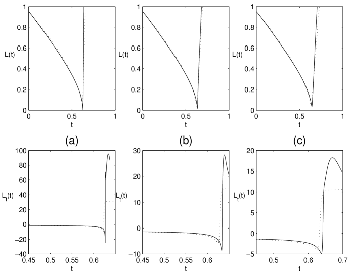
Figure 22: Solution of the damped NLS (55) with $d=1$ and the initial condition $\sqrt{1.05}\psi_{explicit}(t=0,r;T_{c}=1)$ (solid). Dashed line is the solution of the reduced equations (67) with the initial condition $\beta(0)\approx 0.3242$, $L(0)\approx 0.9524$, and $L_{t}(0)=-1.02$. (a) $\delta=10^{-3}$. (b) $\delta=1.5\cdot 10^{-3}$. (c) $\delta=2\cdot 10^{-3}$. Top row: $L(t)$. Bottom row: $L_{t}(t)$.

10 Complex-Ginzburg Landau continuation

The two-dimensional Complex Ginzburg-Landau equation (CGL)

$$i\psi_{t}(t,x,y)+\Delta\psi+|\psi|^{2}\psi-i\epsilon_{1}\psi-i\epsilon_{2}\Delta\psi+i\epsilon_{3}|\psi|^{2}\psi=0,$$

arises in a variety of physical problems: Models of chemical turbulence, analysis of Poiseuille flow, Rayleigh-Bérnard convection and Taylor-Couette flow. Its name comes from the field of superconductivity, where it models phase transitions of materials between superconducting and non-superconducting phases.

In [33], Fibich and Levy showed that as $\epsilon_{1},\epsilon_{2},\epsilon_{3}\longrightarrow 0$, the collapse dynamics is governed, to leading order, by the reduced equations (65) with

$$\tilde{\delta}=\frac{2P_{\rm cr}}{M}(\epsilon_{2}+2\epsilon_{3}).$$

Therefore, Continuation Results 4 and 5 hold also for the CGL continuation of the critical NLS.

11 Continuation in the linear Schrödinger equation

It is well known that in the linear Schrödinger equation, under the geometrical-optics approximation, a focused input beam becomes singular at the focal point. When, however, diffraction is not neglected, the focused beam does not collapse to a point, but rather narrows down to a positive diffraction-limited width, and then spreads out with further propagation. Therefore, diffraction can play the role of ”viscosity” in the continuation of singular geometrical-optics linear solutions. In what follows, we compare this continuation with those in the nonlinear case.

Consider the d-dimensional linear Schrödinger equation

$$2ik_{0}\psi_{t}({\bf x},t)+\Delta\psi=0,\qquad{\bf x}=(x_{1},...,x_{d}),$$ (109a)

with a focused Gaussian initial condition

$$\psi_{0}({\bf x})=e^{-r^{2}/2}e^{-ik_{0}r^{2}/2F},\qquad r=|{\bf x}|,$$ (109b)

where $F>0$ is the focal point. We can look for a solution of the form

$$\psi({\bf x},t)=A({\bf x},t)e^{ik_{0}S({\bf x},t)},$$ (110)

where A and $S$ are real. Substitution in equation (109) gives

$$\left(\nabla S\right)^{2}+2S_{t}-\frac{1}{k_{0}^{2}}\frac{\Delta A}{A}=0,$$ (111a)

and

$$\left(A^{2}\right)_{t}+\nabla S\cdot\nabla\left(A^{2}\right)+A^{2}\Delta S=0,$$ (111b)

with initial conditions

$$S({\bf x},0)=-\frac{r^{2}}{2F},\qquad A^{2}({\bf x},0)=e^{-r^{2}}.$$ (112)

Since $k_{0}\gg 1$, we can apply the geometrical-optics approximation, and neglect the diffraction term $\Delta A$. In this case, equation (111a) becomes

$$\left(\nabla S\right)^{2}+2S_{t}=0,$$ (113)

while equation (111b) remains unchanged.

The solution of equations (111b,  113), subject to the initial conditions (112), is given by

$$S=\frac{r^{2}}{2}\frac{L_{t}}{L},\qquad A^{2}({\bf x},t)=\frac{1}{L^{d}(t)}e^{-\frac{r^{2}}{L^{2}(t)}},\qquad L(t)=1-\frac{t}{F}.$$

Therefore, under the geometrical-optics approximation, the solution of (109) is given by

$$\psi^{go}_{lin}(t,{\bf x})=\frac{1}{L_{go}^{d/2}(t)}e^{-\frac{1}{2}\frac{r^{2}}{L_{go}^{2}(t)}}e^{ik_{0}\frac{r^{2}}{2}\frac{L^{\prime}_{go}(t)}{L_{go(t)}}}\quad,\qquad 0\leq t<F,$$ (114a)

where

$$L_{go}(t)=1-\frac{t}{F}.$$ (114b)

Since $\lim_{t\rightarrow F}|\psi^{go}_{lin}|^{2}=\|\psi_{0}\|^{2}_{2}\cdot\delta({\bf x})$, the geometrical-optics solution becomes singular at the focal point $t=F$.

Equation (109) can also be solved exactly, (i.e., without making the geometrical-optics approximation), yielding

$$\psi_{lin}(t,{\bf x})=\frac{1}{L^{d/2}(t)}e^{-\frac{1}{2}\frac{r^{2}}{L^{2}(t)}}e^{ik_{0}\frac{r^{2}}{2}\frac{L_{t}}{L}+i\tau(t;k_{0})},$$ (115)

where

$$L(t;k_{0})=\sqrt{\frac{1}{F}\frac{(t-t_{min})^{2}}{t_{min}}+L^{2}_{min}},\qquad\tau(t;k_{0})=-\frac{d}{2}\left[\mbox{atan}\left(\frac{t-t_{min}}{L_{min}\sqrt{F\cdot t_{min}}}\right)+\mbox{atan}\left(\frac{k_{0}}{F}\right)\right],$$ (116)

and

$$t_{min}=\frac{F}{1+F^{2}/k_{0}^{2}},\qquad L_{min}=\frac{F}{\sqrt{F^{2}+k_{0}^{2}}}.$$

Since $L(t;k_{0})$ does not shrink to zero at any $t>0$, $\psi_{lin}$ exists for all $0\leq t<\infty$, and in particular for $t>F$.

It is easy to verify that the limiting width of $\psi_{lin}$ is given by

$$\lim_{k_{0}\rightarrow\infty}L(t;k_{0})=|L_{go}(t)|.$$ (117)

In addition, since $\lim_{k_{0}\rightarrow\infty}t_{min}=F$ and $\lim_{k_{0}\rightarrow\infty}L_{min}=0$, then

$$\lim_{k_{0}\rightarrow\infty}\tau(t;k_{0})=\left\{\begin{array}[]{l l}0&\quad 0\leq t<F,\\ -\frac{d}{2}\cdot\pi&\quad F<t<\infty.\end{array}\right.$$ (118)

Therefore,

Lemma 14.

$$\lim_{k_{0}\rightarrow\infty}\psi_{lin}(t,{\bf x})=\left\{\begin{array}[]{l l}\psi_{lin}^{go}(t,{\bf x})&\quad 0\leq t<F,\\ \left(\psi_{lin}^{go}\right)^{\ast}(2F-t,{\bf x})e^{-i\frac{d}{2}\cdot\pi}&\quad F<t<\infty.\end{array}\right.$$ (119)

Hence, $\lim_{k_{0}\rightarrow\infty}\psi$ coincides with $\psi^{go}_{lin}$ before the focal point. Beyond the focal point, there is a bounded jump in the limiting phase, and the continuation is symmetric with respect to $T_{c}=F$. This symmetry is to be expected, since the linear continuation is invariant under (35).

By (118), the limiting phase is unique, both before and after the singularity. This is the opposite from the nonlinear case, where the limiting phase is non-unique beyond the singularity. We thus conclude that

Conclusion 2.

The post-collapse non-uniqueness of the phase is a nonlinear phenomena.

11.1 Simulations

In order to illustrate these results numerically, in Figure 23(a) we plot $L(t;k_{0})$, and observe that it approaches $|L_{go}(t)|$ as $k_{0}\rightarrow\infty$, both before and after the singularity point at $t=F$. In Figure 23(b) we plot $\tau(t;k_{0})=\arg\psi(t,0;k_{0})$ as a function of $t$, and observe that as $k_{0}$ increases, $\tau(t;k_{0})$ approaches the step function (118).

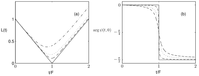
Figure 23: Solution of the linear Schrödinger (109) with $d=1$ and $F=4$. (a): Width $L(t)$, see (116), for $k_{0}=10$ (dashes-dots), $k_{0}=20$ (dots) and $k_{0}=35$ (dashes). Solid line is $|L_{go}(t)|=\left|1-\frac{t}{F}\right|$. (b): $\arg\psi(t,0;k_{0})$ as a function of $t$ for $k_{0}=50$ (dashes), $k_{0}=100$ (dots) and $k_{0}=500$ (dashes-dots). Solid line is (118).

12 Discussion

In this study, we presented several ”old” continuations and four novel continuations of NLS solutions. At this stage, it is not clear whether any of these continuations is the “physical” one. In fact, it is possible that there is no ”universal continuation”, i.e, that different physical setups calls for different continuations.

This study suggests that all continuations share the property that the post-collapse phase becomes non-unique. Indeed, this property follows from the fact that the phase of the singular solution becomes infinite at the singularity, and is thus independent of the specific continuation which is used. Therefore, even without knowing the ”correct” continuation, we can conclude that interactions between post-collapse filaments are chaotic.

Since the Bourgain-Wang blowup solutions are unstable, they are typically classified as “non-generic” solutions. This study shows, however, that these solutions are “generic”, in the sense that they arise as the sub-threshold power continuation of NLS solutions, both before and after the singularity.

It is instructive to compare this study with [4]. In [4], Merle, Raphael and Szeftel showed that the Bourgain-Wang blowup solutions lie on the boundary of an $H^{1}$ open set of global solutions that scatter forward and backward in time, and also on the boundary of an $H^{1}$ open set of solutions that undergo a loglog blowup in finite time. This result follows immediately from the reduced equations (26)–(27) of the sub-threshold power continuation, see Section 4.2, since

• The Bourgain-Wang blowup solutions correspond to $\beta(0)=0$.

• For any $\beta(0)<0$, $L(t)$ remains strictly positive and satisfies $\lim_{t\to\pm\infty}L(t)=0$.

• For any $\beta(0)>0$, $L(t)$ goes to zero at some finite $T_{c}$, at the loglog rate.

An interesting difference between the approaches of this study and [4], is that Merle, Raphael and Szeftel start from the Bourgain-Wang solution at the singularity time $T_{c}$, and then find a smooth deformation such that the deformed solutions belong to the above two open sets on either side of the Bourgain-Wang solution. In this study, we start from a generic initial condition $\psi_{0}=K\cdot F({\bf x})$, and obtain the Bourgain-Wang solution as $K\longrightarrow K_{th}$.

The ‘global” picture that emerges from this study is as follows. Consider a stable singular solution of the critical NLS that undergoes a loglog collapse. Since the singular core $\psi_{R^{(0)}}$ approaches a $\delta$-function with power $P_{\rm cr}$, it can be continued with a $\delta$-function filament with power $P_{\rm cr}$. Such a filament singularity can occur when the collapse-arresting mechanism leads to focusing-defocusing oscillations. Since this is the generic effect of conservative perturbations of the critical NLS (such as nonlinear saturation), see [9, Section 4.1.2], we expect that continuations that are based on conservative perturbations of the NLS will lead to a filament singularity.

When the collapse-arresting mechanism is non-conservative (e.g., nonlinear damping), the solution defocuses (scatters) after its collapse has been arrested, since its power gets below $P_{\rm cr}$. Therefore, we expect that continuations that are based on non-conservative perturbation of the NLS will lead to a point singularity. In addition, the same arguments as in the proof of Continuation Result 2 suggest that non-conservative continuations of solutions that undergo a loglog collapse have an infinite-velocity expanding core.

In Continuation Result 2 we saw that when the continuation leads to a point singularity and is time-reversible, the continuation is symmetric with respect to $T_{c}$ (Property 1). For this to occur, however, the continuation should be conservative (in order to be time reversible), yet it should not lead to focusing-defocusing oscillations. While this holds for the sub-threshold power and the shrinking-hole continuations, it is not expected to hold for conservative perturbations of the NLS, which generically lead to a focusing-defocusing oscillations, hence to a filament singularity. Therefore, we expect that continuations which are based on perturbations of the NLS equation are asymmetric with respect to $T_{c}$. Hence, we believe that Property 1 is non-generic.

Acknowledgment

We acknowledge useful discussions with Frank Merle. This research was partially supported by grant $1023/08$ from the Israel Science Foundation (ISF).