Phase diagram of the XXZ ferrimagnetic spin-(1/2, 1) chain in the presence of transverse magnetic field

Abstract

We investigate the phase diagram of an anisotropic ferrimagnetic spin-($1/2,1$) in the presence of a non-commuting (transverse) magnetic field. We find a magnetization plateau for the isotropic case while there is no plateau for the anisotropic ferrimagnet. The magnetization plateau can appear only when the Hamiltonian has the U(1) symmetry in the presence of the magnetic field. The anisotropic model is driven by the magnetic field from the Néel phase for low fields to the spin-flop phase for intermediate fields and then to the paramagnetic phase for high fields. We find the quantum critical points and their dependence on the anisotropy of the aforementioned field-induced quantum phase transitions. The spin-flop phase corresponds to the spontaneous breaking of Z₂ symmetry. We use the numerical density matrix renormalization group and analytic spin wave theory to find the phase diagram of the model. The energy gap, sublattice magnetization, and total magnetization parallel and perpendicular to the magnetic field are also calculated. The elementary excitation spectrums are obtained via the spin wave theory in the three different regimes depending on the strength of the magnetic field.

I Introduction

Quantum ferrimagnets are a general class of strongly correlated magnetism, which have attracted much interest in experimental as well as theoretical investigations. Examples of such realizations are the bimetallic molecular magnets like CuMn(S₂C₂O₂)₂(H₂O)${}_{3}\cdot$4.5H₂O and numerous bimetallic chain compounds which have been synthesized systematically Gleizes 81 ; Pei 87 . In these materials, the unit cell of the magnetic system is composed of two spins, the smaller one is $\sigma=1/2$ and the larger one ($\rho$) is changed from $1/2$ to $5/2$. The magnetic and thermodynamic properties of these models are different from the homogeneous spin counterparts. For instance, the one dimensional mixed-spin model represents a ferromagnetic behavior for the low temperature regime while a crossover appears to the antiferromagnetic behavior as temperature increases Pati 97 ; Yamamoto 99 ; Kolezhuk 99 ; Jahan2004 ; Jahan2006 . The crossover can be explained in terms of the two elementary excitations where the lower one has the ferromagnetic nature and a gapped spectrum above it with antiferromagnetic property Yamamoto 98 . Moreover, the mixed spin models have shown interesting behavior for the quasi one dimensional lattices (ferrimagnetic ladders). Despite that the two-leg spin-1/2 ladder is gapful, representing a Haldane phase, the two-leg (mixed spin) ferrimagnet is always gapless with the ferromagnetic nature in the low energy spectrum. However, a special kind of dimerization can drive the ferrimagnetic ladder to a gapped phase Langari 00l ; Langari 01 .

The presence of a longitudinal magnetic field preserves the U(1) symmetry of the XXZ interactions and creates a nonzero magnetization plateau in a one-dimensional ferrimagnet for small magnetic fields in addition to the saturation plateau for large magnetic fields Alcaraz 97 ; Sakai 99 ; Abolfath 01 . The former plateau corresponds to the opening of the Zeeman energy gap which removes the high degeneracy of the ground state subspace. The ferrimagnets on ladder geometry present a rich structure of plateaus depending on the ratio and dimerization of exchange couplings Langari 00p . In both one-dimensional and two-leg ferrimagnets the magnetization plateaus can be understood in terms of the Oshikawa, Yamanaka and Affleck (OYA) argument OYA because the longitudinal magnetic field commutes with the rest of the Hamiltonian and the models have U(1) symmetry. However, the situation is different when a transverse magnetic field is applied on the system, because the transverse field does not commute with the XXZ interaction and breaks the U(1) symmetry of the model. The onset of a transverse field develops an energy gap in a spin-1/2 chain which initiates an antiferromagnetic order perpendicular to the field direction Dmitriev 02 ; Essler 03 ; Langari 04 ; Dmitriev 04 . The ordered phase is a spin-flop phase because of nonzero magnetization in the field direction; however, there is no magnetization plateau even in the gapped phase Langari 06 . The lack of U(1) symmetry prohibits the use of the OYA argument, thus prompts the question of a magnetization plateau and the presence of an energy gap Oshikawa2000 in the spectrum.

The structure of the paper is as follows. First we study the anisotropic ferrimagnetic chain in the presence of a transverse magnetic field by using the density matrix renormalization group (DMRG) White1993 and exact diagonalization Lanczos methods. The energy gap, sublattice magnetization, and total magnetization in both parallel and perpendicular to the field direction are presented in Sec. II. We further address the energy gap behavior versus the magnetic field and the magnetization plateau. The phase diagram of the model is also presented in the same section. We then use an analytical tool, the spin wave theory (SWT), to obtain the low energy excitation spectrum of the model in Sec. III. The SWT is applied in three different regions depending on the strength of the magnetic field. The qualitative behavior of the model is explained in terms of SWT and the magnetization is compared with DMRG results. The results of SWT help to explain the energy gap behavior of DMRG data. We finally summarize our results in Sec. IV, where we put together both quantitative DMRG and qualitative SWT results to analyze the different phases of the model in the presence of a transverse magnetic field.

II Density Matrix Renormalization Group results

We have implemented the numerical DMRG technique to study the magnetic properties of the anisotropic ferrimagnetic spin-($1/2,1$) chain in the presence of a transverse magnetic field given by the Hamiltonian (1):

$$H=J\sum_{i=1}^{N}[\sigma^{x}_{i}\rho^{x}_{i}+\sigma^{y}_{i}\rho^{y}_{i}+\sigma^{x}_{i}\rho^{x}_{i+1}+\sigma^{y}_{i}\rho^{y}_{i+1}+\Delta(\sigma^{z}_{i}\rho^{z}_{i}+\sigma^{z}_{i}\rho^{z}_{i+1})-h(\sigma^{x}_{i}+\rho^{x}_{i})],$$ (1)

where $\sigma_{i}^{\alpha}$ ($\rho_{i}^{\alpha}$) represents the $\alpha$-component of spin operators at site $i$ for spin amplitude $\sigma=1/2$ ($\rho=1$). The antiferromagnetic exchange coupling is $J>0$, the anisotropy is defined by $\Delta$, and $h$ is proportional to the strength of the transverse magnetic field.

The DMRG computations have been done on an open chain of length $108$ spins ($N=54$ unit cells) and the number of states kept in each step of DMRG is $300\leq m\leq 500$. We have also studied the chains with larger lengths (up to $N=100$) and observed no significant changes on the data of magnetization and staggered magnetization within 5 digits of accuracy.

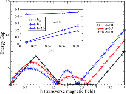
Figure 1: The energy gap versus the transverse magnetic field. Different plots belong to various values of the anisotropy parameter $\Delta=0.0,0.5.1.0$. Inset: The scaling of gap versus $(2N)^{-1}$ for $\Delta=0.0$ at two critical points $h_{c1}$ and $h_{c2}$ confirms the vanishing of gap at these points while its scaling at $h=2.0$ verifies a finite gap in the thermodynamic limit ($N\rightarrow\infty$).

The energy gap is defined as the difference between the first excited state energy and the ground state energy. It shows whether the model is gapless or gapful depending on its zero or nonzero value, respectively. Using the DMRG computations, we have plotted in Fig. 1 the energy gap of the model versus the transverse magnetic field for different values of anisotropy parameter, $\Delta=0,0.5,1.0$. All plots show a gapped phase for small values of the magnetic field, $h<h_{c1}(\Delta)$, and a paramagnetic gapped phase for $h>h_{c2}(\Delta)$. The gap vanishes at two critical points, $h=h_{c1}(\Delta)$ and $h=h_{c2}(\Delta)$. The isotropic case ($\Delta=1$) remains gapless in the intermediate region $h_{c1}(\Delta)<h<h_{c2}(\Delta)$, while the anisotropic case ($\Delta\neq 1$) is gapful. The gap behaves differently for various $\Delta$ in the small-field and intermediate-field gapped phase.

In the isotropic case $\Delta=1$, the behavior of gap versus $h$ can be explained in terms of the elementary excitations of the model. For $\Delta=1$, the U(1) symmetry of the model is restored and the magnetic field operator commutes with the rest of the Hamiltonian. Thus, the energy spectrum for $\Delta=1$ is expressed in terms of the spectrum at $h=0$ plus a shift of energy which depends on $h$. At $h=0$ the model has SU(2) symmetry and the ground state is a ferromagnetic state with total spin $S_{G}=N(|\rho-\sigma|)$, which is highly degenerate and the lowest ferromagnetic spectrum is a gapless one, namely $\nu^{-}(k)$ [see Eq. (17)]. An antiferromagnetic spectrum ($\nu^{+}(k)$) exists above the ferromagnetic one, and the lowest state of the antiferromagnetic spectrum has total spin $S_{AF}=S_{G}+1$ with a finite gap $2J|\rho-\sigma|$, measured from the ground state. Upon adding a commuting magnetic field to the ferrimagnetic chain the symmetry is lowered to U(1) and the energy levels are affected by a Zeemann term, i.e., $-hS^{x}$. For the magnetic fields smaller than $\overline{h}$ (which will be defined later), the Zeeman energy gain of the ground state is larger than all of the other states in the ferromagnetic spectrum; thus the ground state remains robust, and the first excited state is the first state in the ferromagnetic spectrum (with energy $J(\nu^{-}(k)+h)$), which leads to the energy gap equal to $Jh$. This explanation remains valid until the gain of the Zeeman term of the lowest state of the antiferromagnetic spectrum ($J(\nu^{+}(k)-h)$) dominates the gain of the first excited state in the ferromagnetic spectrum. It defines $\overline{h}$ by the following equation:

$$\nu^{-}(k)+\overline{h}=\nu^{+}(k)-\overline{h},$$ (2)

which gives $\overline{h}=|\rho-\sigma|$ within linear approximation of SWT (from which both $\nu^{\pm}(k)$ will be derived in the next sections). At this point, the first excited state is the lowest state of the antiferromagnetic spectrum. Thus, the energy gap behaves as ($2J|\rho-\sigma|-Jh$) before it vanishes at $h=h_{c1}(\Delta=1)=2|\rho-\sigma|$. The linear increasing behavior for small fields and then linear decreasing of the energy gap are clear in the DMRG data for $\Delta=1$, shown in Fig. 1. Although the DMRG values for $\overline{h}$ and $h_{c1}$ have some discrepancies with those obtained by linear SWT, the SWT gives the qualitative behavior correctly.

The energy gap of the anisotropic Hamiltonian ($\Delta\neq 1$) is defined as $E_{1}-E_{0}$ for $0<h<h_{c1}$ and $h>h_{c2}$, where $E_{1}$ is the first excited state energy and $E_{0}$ is the ground state energy. However, the ground state becomes degenerate ($E1=E_{0}$) for $h_{c1}\leq h\leq h_{c2}$, where the energy gap is the difference between the second excited state energy and the ground state one, $E_{2}-E_{0}$. For small magnetic fields the scaling behavior of the energy gap can be explained using the quasi-particle excitations of the model as $h\rightarrow 0$. The leading term of quasi-particle excitations for very small magnetic fields ($h\rightarrow 0$) gives the scaling of energy gap as $\sqrt{h}$, for $\Delta\neq 1$ [in the weak field SWT, Eq.(18)]. In a similar manner, the leading term of the strong field SWT [Eq.(21)] leads to linear dependence of the gap on the magnetic field in the paramagneic phase which explains very well the behavior in Fig. 1. The linear dependence of gap versus the magnetic field for $h>h_{c2}$ is confirmed by the DMRG numerical data for any isotropies.

We have plotted the energy gap versus $(2N)^{-1}$ in the inset of Fig. 1 to observe its finite size scaling (where $2N$ is the total number of spins). We have implemented both the Lanczos and DMRG algorithms to calculate the energy gap for $\Delta=0$. We have plotted the minimum value of gap which occurs at $h_{c1}$ and $h_{c2}$ versus $(2N)^{-1}$ which clearly shows that the gap vanishes in the thermodynamic limit ($N\rightarrow\infty$). It suggests that both $h_{c1}$ and $h_{c2}$ correspond to quantum critical points. The different magnetization characteristic confirms that a quantum phase transition occurs at both $h_{c1}$ and $h_{c2}$ (see Fig. 2). We have also plotted the energy gap for $h=2.0$ to justify that the gap of the intermediate region is finite in the thermodynamic limit.

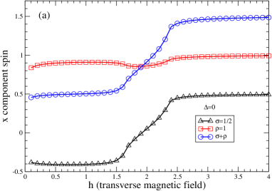
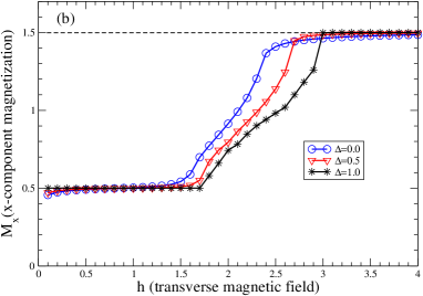
Figure 2: (a) The $x$-component sublattice magnetization versus a transverse magnetic field for both $\sigma=1/2$ and $\rho=1$ spins and their sum as the unit cell magnetization in $x$-direction for anisotropy parameter $\Delta=0$. (b) The $x$-component unit cell magnetization versus a transverse magnetic field for different anisotropies $\Delta=0.0,0.5,1.0$. The dashed line shows the saturation value at $M_{x}=3/2$.

We have also plotted the $x$-component magnetization of each sublattice in Fig. 2-(a) for ferrimagnetic spin-$(1/2,1)$ chain with $\Delta=0$ versus $h$ employing the DMRG technique. The total magnetization has been plotted in Fig. 2-(b) for different values of anisotropy, $\Delta=0,0.5,1.0$. To calculate the magnetization we have considered those spins which are far from the open ends of the chain to avoid the finite size boundary conditions. In this respect, ten spins have been neglected from each side of the open chain and the magnetization has been averaged over the rest of spins. Figure 2-(b) shows the possibility of two plateaus in the magnetization along the field direction. For the isotropic case ($\Delta=1$), it can be explained in terms of the OYA argument OYA . According to this argument, $n(S-m)=\mbox{integer}$, where $n$ is the periodicity of the ground state, $S$ the total spin of unit cell, and $m$ a possible magnetization plateau of the unit cell, the one-dimensional spin-($1/2,1$) chain can show two plateaus at $m=1/2$ and $3/2$. However, for $\Delta\neq 1$ the axial symmetry of the model is broken by the transverse magnetic field, and the OYA argument is not applicable. Thus, more investigations is required to figure out the difference between the anisotropic ($\Delta\neq 1$) and isotropic ($\Delta=1$) cases.

To get more knowledge on the behavior of magnetization for the anisotropic case, we have plotted the total magnetization in the magnetic field direction ($M_{x}$) versus the anisotropy parameter ($\Delta$) for small magnetic field values in Fig. 3. The plots have been shown for those values of the magnetic field which seems to exhibit the magnetization plateaus. Figure 3 clearly verifies that the magnetization plateau only exists for the isotropic case, while there is no plateau for $\Delta\neq 1$. The magnetization per unit cell ($M_{x}$) in the direction of magnetic field ($h$) is given by

$$M_{x}=-\frac{1}{N}\frac{\partial E_{0}}{\partial h},$$ (3)

where $E_{0}$ is the ground state energy. The above relation for a gapped phase simply states that if the ground state energy is linear in the magnetic field ($E_{0}\propto h$), the magnetization will be constant, (the presence of plateau); otherwise the magnetization will depend on the magnetic field, (the absence of plateau). Let write the Hamiltonian as $H=H_{0}-hH_{1}$ where $H_{0}$ is the XXZ interacting part and $hH_{1}$ is the magnetic field part. In the presence of U(1) symmetry ($\Delta=1$) the interacting and the magnetic field parts commute $[H_{0},H_{1}]=0$. Thus, $E_{0}$ is a linear function of $h$ which leads to the emergence of a magnetization plateau when the energy gap is nonzero. This agrees with the OYA statement. However, the transverse magnetic field breaks the U(1) symmetry in the anisotropic case ($\Delta\neq 1$) and $[H_{0},H_{1}]\neq 0$. Therefore, the ground state energy depends on $h$ non-linearly which gives a change of magnetization when $h$ varies, i.e. the lack of magnetization plateau even if a finite energy gap exists.

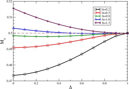
Figure 3: Unit cell magnetization ($M_{x}$) versus the anisotropy parameter ($\Delta$) for some low magnetic field values ($h$). Our plots justify the plateau only for $\Delta=1$. The dashed line represents $M_{x}=0.5$ (the plateau value).

Although the above general explanation is applied to the strong magnetic field regime the saturated plateau ($M_{x}=1.5$) can also be explained from another point of view. An eigenstate with full saturation is classified as a factorized state Rezai 10 in which all spins align in the direction of the magnetic field. As a general argument, it has been shown in Ref. Rezai 10 that the full saturation for an anisotropic Heisenberg type interaction in the presence of a magnetic field takes place at a finite value of the magnetic field if the model is rotationally invariant around the field direction. Accordingly, the saturation at $M_{x}=1.5$ takes place only for the isotropic case ($\Delta=1$) and $h\geq h_{c2}$. In the anisotropic case ($\Delta\neq 1$), the fully polarized plateau can take place for infinite strong magnetic field while the nearly saturated state, ($M_{x}\simeq 1.5$), can be observed for large magnetic fields. To justify this argument we have plotted the $x$-component magnetization of each unit cell for different values of $\Delta$ in Fig. 2-(b). It is clear that the magnetization in the field direction does not reach the saturation value of $M_{x}=1.5$ for $\Delta=0$ and $0.5$, while it obviously touches its saturated value for $\Delta=1$ and $h\geq 3$.

The antiferromagnetic interactions between the spins in each unit cell make them to be antiparallel, which leads to the total $x$-component magnetization $M_{x}=\langle\sigma_{x}+\rho_{x}\rangle\simeq 0.5$. This phase has been shown schematically in Fig. 4-(1) where we have neglected the effects of small quantum fluctuations on the directions of the spins. The non-commuting transverse magnetic field opens a gap which is robust as long as $h<h_{c1}$. This (gapped) Néel phase corresponds to the first plateau at $M_{x}=0.5$ for $\Delta=1$ and a semi-plateau ($M_{x}\simeq 0.5$) for $\Delta\neq 1$. By further increasing $h$, the gap is closed at the first critical field $h_{c1}(\Delta)$ (for $\Delta=0$, $h_{c1}\simeq 1.6$) where the magnetization starts to increase obviously. Further increasing of the magnetic field leads to a continuous change of the ground state property which gives a gradual change of the magnetization-Fig. 4-(2-4). For strong magnetic field ($h_{c2}(\Delta=0)\gtrsim 2.4$) the spins are nearly aligned in the direction of the magnetic field, the semi-plateau at $M_{x}\simeq 1.5$ [Fig. 2-(a) and Fig. 4-(5)].

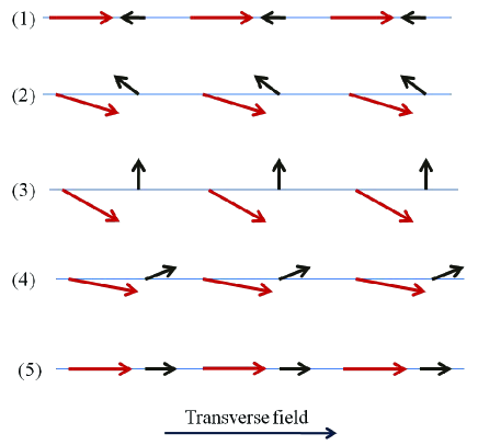
Figure 4: Schematic of spins’ orientations in different phases of the anisotropic ferrimagnetic spin-($1/2,1$) chain in the presence of a transverse magnetic field.

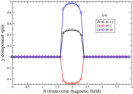
Figure 5: The $y$-component sublattice magnetization versus the transverse magnetic field for $\Delta=0$. This component is nonzero only in the intermediate phase $1.6\lesssim h\lesssim 2.4$. Moreover, the $y$-component spins are exactly equal and antiparallel for both sublattices. The staggered magnetization of the unit cell in the $y$ direction is nonzero within the intermediate region.

To get more insight on the ground state properties of the model, we have plotted the $y$-component spin expectation value versus the transverse magnetic field in Fig. 5 for $\Delta=0$. The magnetization in the $y$ direction for both sublattice spins is zero for $h\lesssim 1.6$ and $h\gtrsim 2.4$; however, it becomes nonzero in the intermediate region $1.6\lesssim h\lesssim 2.4$. The values of the $y$ component spins in the unit cell are equal, and their directions are opposite to each other, $\langle\sigma^{y}\rangle=-\langle\rho^{y}\rangle$. It is surprising that for any value of the magnetic field $1.6\lesssim h\lesssim 2.4$ we get $\langle\sigma^{y}\rangle=-\langle\rho^{y}\rangle$ whereas the spin magnitude on the sublattices are different ($\sigma\neq\rho$). At the factorizing field, $h_{f}\simeq 2.24$ (which will be explained in the next section), where the condition $\sigma\sin|\theta|=-\rho\sin|\beta|$ should be satisfied, the mentioned relation is obtained $\langle\sigma^{y}\rangle=-\langle\rho^{y}\rangle$. The staggered magnetization in the $y$ direction, $SM_{y}=\langle\sigma^{y}-\rho^{y}\rangle$, is nonzero for this region. Moreover, our numerical data verifies that the $z$ component magnetization on both sublattices is zero for any value of the magnetic field.

Generally, let us consider the $y$ component staggered magnetization as an order parameter, which is nonzero for $h_{c1}(\Delta)<h<h_{c2}(\Delta)$ and zero elsewhere. Nonzero $SM_{y}$ corresponds to a spontaneous breaking of Z₂ symmetry. In fact, for any value of $\Delta$ the model has a Z₂ symmetry which can be expressed by the parity operator $P=\otimes_{i}\sigma_{i}^{x}\rho_{i}^{x}$. This symmetry, which can also be considered as a $\pi$ rotation around the magnetic field direction ($x$), leads to vanishing value for the $z$ and $y$ components of the spins. However, the symmetry is spontaneously broken for $h_{c1}(\Delta)<h<h_{c2}(\Delta)$ which selects one of the parity eigenkets to give nonzero sublattice magnetization in the $y$ direction.

III Spin wave analysis

We have applied the spin wave theory to get more knowledge and a qualitative picture of the phase diagram. The SWT is a method to describe a spin model in terms of boson operators. The elementary excitations of the spin model are given by bosonic quasi-particles which are constructed on a given background. Based on this fact the SWT can be considered on different backgrounds to build up a bosonic system. Typically, a state in the Hamiltonian Hilbert space is considered as the background which is supposed to be the ground state within an approximation. However, there exists some spin models such as the isotropic antiferromagnetic Heisenberg spin-1/2 chain that do not have an ordered ground state, and thus the SWT fails to explain the properties of the model correctly. Therefore, the existence of an exact ground state is a good starting point to initiate a spin wave analysis.

The ferrimagnetic chain both in the absence and presence of longitudinal magnetic fields has been studied by the SWT Pati 97 ; Yamamoto 99 ; Kolezhuk 99 ; Yamamoto 98 ; Sakai 99 ; Abolfath 01 . Although the Néel state is not the exact ground state for a ferrimagnet in the presence of a longitudinal field, the SWT gives a good description of the model which justifies that the quantum fluctuations are not strong enough to ruin the whole picture. It would be more interesting to initiate a spin wave theory based on an exact ground state for a ferrimagnet in the presence of a transverse magnetic field. According to Ref. Rezai 10 , the exact ground state of a general class of ferrimagnets can be found at the factorizing magnetic field, $h=h_{f}$. This ground state is a factorized state, which is a perfect background to implement SWT. It gives a reliable analysis around $h=h_{f}$ (see next subsection). We will also study the SWT for small and large magnitudes of the magnetic field. Our analysis is limited to the linear spin wave approximation to get the magnetic properties of the spin-($\sigma,\rho$) ferrimagnets in the presence of a transverse magnetic field.

III.1 SWT at $h=h_{f}$

Let us briefly introduce the exact factorized ground state of a ferrimagnet in the presence of a magnetic field Rezai 10 . The factorized ground state for the Hamiltonian of Eq. (1) can be written in the following form:

$$|\psi_{0}\rangle=\bigotimes_{i\in A_{\sigma},j\in B_{\rho}}|\sigma^{\prime}_{i}\rangle|\rho^{\prime\prime}_{j}\rangle,$$ (4)

where $|\sigma^{\prime}_{i}\rangle$ and $|\rho^{\prime\prime}_{j}\rangle$ are the eigenstates of $\vec{\sigma}_{i}\cdot\hat{n}_{i}^{\prime}$ and $\vec{\rho}_{j}\cdot\hat{n}_{j}^{\prime\prime}$ with the largest eigenvalues, respectively, with $\hat{n}_{i}^{\prime}$ and $\hat{n}_{j}^{\prime\prime}$ being unit vectors pointing in polar angles ($\theta,\varphi=0$) and ($\beta,\alpha=0$). $A_{\sigma}$ and $B_{\rho}$ represent the two sublattices which contain the two different spins. The factorized state is called a bi-angle state, defined by the two angles ($\theta,\beta$) and represents the ground state of the model at $h=h_{f}$, where

$$\cos\beta = \frac{\rho+\Delta\sigma}{\sqrt{\rho^{2}+\sigma^{2}+2\Delta\rho\sigma}},$$

$$\cos\theta = \frac{\sigma+\Delta\rho}{\sqrt{\rho^{2}+\sigma^{2}+2\Delta\rho\sigma}},$$ (5)

and

$$h_{f}=2\sqrt{\rho^{2}+\sigma^{2}+2\Delta\sigma\rho},$$

$$\epsilon_{f}=-(\sigma^{2}+\rho^{2}+\Delta\sigma\rho),$$ (6)

with $\epsilon_{f}$ being the ground state energy per site at the factorizing field.

To perform the spin wave analysis around $h=h_{f}$, we first implement a rotation on the original Hamiltonian ($H$). The rotated Hamiltonian ($\tilde{H}$) is the result of rotations on all lattice points of $H$, and is given by the following relations

$$\tilde{H} = \tilde{D}^{{\dagger}}H\tilde{D},$$

$$\tilde{D} = \bigotimes_{i\in A_{\sigma},j\in B_{\rho}}D_{i}^{\sigma}(0,\theta,0)D_{j}^{\rho}(0,\beta,0).$$ (7)

The rotation operator

$$D^{\rho}(0,\beta,0)=D(\alpha=0,\beta,\gamma=0)=D_{z}(\alpha)D_{y}(\beta)D_{z}(\gamma),$$

is defined in terms of Euler angles, and a similar expression is considered for $D^{\sigma}(0,\theta,0)$.

In the rotated basis defined by ($x^{\prime},y^{\prime},z^{\prime}$) and ($x^{\prime\prime},y^{\prime\prime},z^{\prime\prime}$), the bi-angle state becomes the fully polarized ground state of $\tilde{H}$. In the next step, the rotated Hamiltonian is bosonized via a Holstein-Primakoff (HP) transformation,

$$\sigma^{+}_{i}=\sqrt{2\sigma-a^{{\dagger}}_{i}a_{i}}\ a_{i},\ \ \ \ \ \ \ \ \sigma^{x^{\prime}}_{i}=\sigma-a_{i}^{{\dagger}}a_{i},$$

$$\rho^{+}_{j}=\sqrt{2\rho-b^{{\dagger}}_{j}b_{j}}\ b_{j},\ \ \ \ \ \ \ \ \rho^{x^{\prime\prime}}_{j}=\rho-b^{{\dagger}}_{j}b_{j},$$ (8)

where $a_{i}(a^{\dagger}_{i})$ and $b_{j}(b^{\dagger}_{j})$ are two types of annihilation (creation) boson operators, satisfying the commutation relations: $[a_{i},a_{j}^{\dagger}]=\delta_{i,j}$, $[b_{i},b_{j}^{\dagger}]=\delta_{i,j}$, $[a_{i},b_{j}^{\dagger}]=0$ and $[a_{i},b_{j}]=0$.

The Hamiltonian in the momentum ($k$) space and in the linear spin wave approximation is written as

$$\tilde{H}=E_{1}+\tilde{H}_{1}+\tilde{H}_{2},$$

$$E_{1}=NJ\sigma\rho\cos(\beta-\theta)+NJh(\rho\cos\beta+\sigma\cos\theta),$$

$$\tilde{H}_{1}=J\sum_{k}\biggl{\{}2\sqrt{\rho\sigma}\Delta\cos\frac{k}{2}(a_{k}b_{k}^{{\dagger}}+b_{k}a_{k}^{{\dagger}})$$

$$+\left(\frac{h^{2}_{f}}{2\rho}+\frac{h_{f}\sigma\cos\theta}{\rho}+(h_{f}-h)\cos\beta-2\Delta\sigma\right)b_{k}^{{\dagger}}b_{k}$$

$$+\left(\frac{h^{2}_{f}}{2\sigma}+\frac{h_{f}\rho\cos\beta}{\sigma}+(h_{f}-h)\cos\theta-2\Delta\rho\right)a_{k}^{{\dagger}}a_{k}\biggr{\}},$$

$$\tilde{H}_{2}=J\frac{\sqrt{N}(h_{f}-h)}{\sqrt{2}}\Big{[}\sqrt{\rho}\sin\beta\ (b_{0}+b_{0}^{{\dagger}})$$

$$\;\;\;\;\;\;\;+\sqrt{\sigma}\sin\theta(a_{0}+a_{0}^{{\dagger}})\Big{]},$$

where $N$ is the total number of spins in each sublattice. The unitary transformation that diagonalizes $\tilde{H}_{1}$ is given by

$$\chi_{k} = a_{k}\cos\eta_{k}-b_{k}\sin\eta_{k},$$

$$\psi_{k} = b_{k}\cos\eta_{k}+a_{k}\sin\eta_{k},$$ (10)

where $\chi_{k}$ and $\psi_{k}$ are the quasi-particle boson operators that preserve the bosonic commutation relations. In this representation, we obtain

$$\tilde{H}_{1}=\sum_{k}(\omega^{-}(k)\chi_{k}^{{\dagger}}\chi_{k}+\omega^{+}(k)\psi_{k}^{{\dagger}}\psi_{k}),$$ (11)

in which $\omega^{\pm}$ are the quasi-particle excitation modes. The dispersion relations are given by

$$\omega^{\pm}(k) = JD^{+}\pm J\frac{D^{-}+2\Delta\sqrt{\sigma\rho}\tan(2\eta_{k})\cos\frac{k}{2}}{\sqrt{1+\tan^{2}(2\eta_{k})}},$$ (12)

$$\tan(2\eta_{k})=\frac{2\Delta\sqrt{\rho\sigma}\cos\frac{k}{2}}{D^{-}},$$

in which

$$D^{\pm} \equiv \frac{h^{2}_{f}}{4}(\frac{1}{\rho}\pm\frac{1}{\sigma})+h_{f}(\frac{\sigma}{2\rho}\cos\theta\pm\frac{\rho}{2\sigma}\cos\beta)$$ (13)

$$- \Delta(\sigma\pm\rho)+\frac{h_{f}-h}{2}(\cos\beta\pm\cos\theta).$$

A shift on the zero momentum component of boson operators, defined by two constants $t^{\pm}$, diagonalizes the full Hamiltonian; i.e., $\chi_{0}\rightarrow\chi_{0}+t^{-}\;,\;\psi_{0}\rightarrow\psi_{0}+t^{+}$, where

$$t^{+}=\frac{\sqrt{2N}(h-h_{f})\left(\sqrt{\sigma}\sin\eta_{0}\sin\theta+\sqrt{\rho}\cos\eta_{0}\sin\beta\right)}{2\omega^{+}},$$

$$t^{-}=\frac{\sqrt{2N}(h-h_{f})\left(\sqrt{\sigma}\cos\eta_{0}\sin\theta-\sqrt{\rho}\sin\eta_{0}\sin\beta\right)}{2\omega^{-}}.$$

(14)

The diagonalized Hamiltonian is given by

$$\tilde{H}=E_{gs}+\sum_{k}\bigg{(}\omega^{-}(k)\chi_{k}^{{\dagger}}\chi_{k}+\omega^{+}(k)\psi_{k}^{{\dagger}}\psi_{k}\bigg{)},$$

$$E_{gs}=E_{1}+\omega^{-}t^{-^{2}}+\omega^{+}t^{+^{2}}$$

$$+\sqrt{2N}J(h_{f}-h)\bigg{(}(\sqrt{\sigma}\sin\theta\cos\eta_{0}-\sqrt{\rho}\sin\eta_{0}\sin\beta)t^{-}$$

$$+(\sqrt{\sigma}\sin\theta\sin\eta_{0}+\sqrt{\rho}\cos\eta_{0}\sin\beta)t^{+}\bigg{)},$$

$$E_{f}=2NJ\epsilon_{f}$$ (15)

where $E_{gs}$ is the ground state energy which reduces to $E_{f}$ at the factorizing field ($h_{f}$) (i.e., the energy of the exact bi-angle state).

The magnetic properties of model (1) can be studied through the linear spin wave theory-Eq. (III.1). In Fig. 6-(a), we have plotted the sublattice magnetization of the anisotropic ferrimagnetic spin-($1/2,1$) chain for $\Delta=0.5$. The $x$ and $y$ components of sublattice magnetization are nonzero [Fig. 6-(a)]; however, the $z$-component of the sublattice magnetization is zero, denoting that the spins are located in the $xy$ plane. It should be noted that the values of sublattice magnetization is exact at the factorizing field while it is approximately correct for the magnetic field close to the factorizing field. The $\alpha$-component of total magnetization per unit cell is $M_{\alpha}=\langle\rho^{\alpha}+\sigma^{\alpha}\rangle$ and the corresponding staggered magnetization is defined $SM_{\alpha}=\langle\rho^{\alpha}-\sigma^{\alpha}\rangle$. In Fig. 6-(b), we have plotted the $x$ and $y$ components of total magnetization and staggered magnetization. Around the factorizing field the model has a considerable magnetization in the $x$ direction and a staggered magnetization in the $y$ direction, which identifies a spin-flop phase around the factorizing field. The model has a dual character i.e. it behaves like a ferromagnet in the $x$ direction and like an antiferromagnet in the $y$ direction, it is the result of two branches of excitations, Eq. (III.1), which are the origin of the existence of two dynamics in the model Siah 08 ; Abou 10 . We will discuss later the effects of magnetic field on the configuration of both spins in more details.

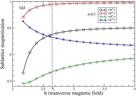
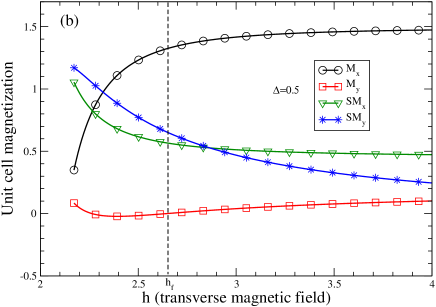
Figure 6: (a) The sublattice magnetization. (b) Magnetization and staggered magnetization per unit cell of the anisotropic ferrimagnetic spin-($1/2,1$) chain versus transverse field, for $\Delta=0.5$. The factorized ground state is chosen as the background in the linear SWT.

III.2 SWT at weak and strong magnetic fields

(a) Weak Field SWT

In the SWT it is assumed that the ground state defines a particular classical direction for the spins. In the weak magnetic fields close to $h=0$, we expect to have a Néel-ordered configuration. Therefore, we use the following Holstein-Primakoff (HP) transformations:

$$\sigma^{+}_{i}=a_{i}^{\dagger}\sqrt{2\sigma-a^{{\dagger}}_{i}a_{i}},\ \ \ \ \ \ \ \ \sigma^{x}_{i}=-\sigma+a_{i}^{{\dagger}}a_{i},$$

$$\rho^{+}_{j}=\sqrt{2\rho-b^{{\dagger}}_{j}b_{j}}\ b_{j},\ \ \ \ \ \ \ \ \rho^{x}_{j}=\rho-b^{{\dagger}}_{j}b_{j}.$$ (16)

In the linear spin wave approximation and within Fourier space representation, one can diagonalize the Hamiltonian which is given by

$$H=E_{0}+\sum_{k}\{\nu^{-}(k)v_{k}^{{\dagger}}v_{k}+\nu^{+}(k)w_{k}^{{\dagger}}w_{k}\},$$ (17)

where

$$E_{0} = -NJ(2\sigma\rho+\rho+\sigma)-NJh(\rho-\sigma)+\frac{1}{2}\sum_{k}(\nu^{-}(k)+\nu^{+}(k)),$$

$$\nu^{\pm}(k)=J\sqrt{2(p^{2}+s^{2}-2\Delta\rho\sigma\cos^{2}\frac{k}{2}\pm D_{1})},$$

$$D_{1} = \sqrt{(p^{2}-s^{2})^{2}-4[\Delta(p^{2}+s^{2})-ps(1+\Delta^{2})]\rho\sigma\cos^{2}\frac{k}{2}}$$

$$p = \rho-\frac{h}{2},\ \ \ \ \ \ \ \ \ \ \ \ \ s=\sigma+\frac{h}{2}.$$ (18)

and $v^{\dagger}_{k},w^{\dagger}_{k}(v_{k},w_{k})$ are bosonic quasi-particle creation (annihilation) operators. The procedure of the diagonalization paraunitary dictates that the bosonic Hamiltonian should be positive definite. This constraint implies that for $|\Delta|\leq 1$ the amount of magnetic field obeys the condition $h<2(\rho-\sigma)$, and for $1\leq|\Delta|<\frac{\rho+\sigma}{2\sqrt{\sigma\rho}}$ the magnetic field should be $|h-\rho+\sigma|<\sqrt{(\rho+\sigma)^{2}-4\rho\sigma\Delta^{2}}.$

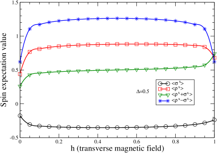
Figure 7: The sublattice magnetization, total magnetization and staggered magnetization per unit cell of the anisotropic ferrimagnetic spin-($1/2,1$) chain versus transverse field, for $\Delta=0.5$, when the Néel order is chosen as the background in the linear SWT.

Let us consider the special case of ($\sigma=\frac{1}{2},\rho=1$) and $\Delta=0.5$. The Hamiltonian of this system (in the linear SWT approximation) is positive definite only for magnetic fields smaller than $h_{0}=1$. Accepting this condition we have plotted in Fig. 7 the sublattices field-induced magnetization, the total magnetization and the staggered magnetization per cell of the whole chain versus transverse field $h$. It shows that for $0<h<1$ the model is affected slightly by the transverse magnetic field. In other words, the staggered magnetization in the $x$ direction is close to its maximum value (the Néel ordered state). The quantum fluctuations for $0<h<1$ are not strong enough to change the magnetization from its zero field value. However, upon reaching $h_{0}=1$ the quantum fluctuations are suddenly increased so that they destroy the ordered state completely. Thus within this linear SWT, the first critical field is $h^{SWT}_{c1}=h_{0}=1$ and for an arbitrary ($\sigma,\rho$)-ferrimagnetic chain it becomes $h^{SWT}_{c1}=2|\rho-\sigma|$. Although $h^{SWT}_{c_{1}}$ does not depend on the anisotropy parameter $\Delta$ and is slightly different from the DMRG results (Fig. 2), the linear SWT describes the elementary excitations of the model well.

(b) Strong Field SWT

For the strong magnetic fields the ground state is ordered in the direction of the magnetic field. The fully polarized ground state in which all spins are aligned in the field direction is used as the background for initiating the SWT. In this case the following HP transformation is implemented for the spin operators

$$\sigma^{+}_{i}=\sqrt{2\sigma-a^{{\dagger}}_{i}a_{i}}\ a_{i},\ \ \ \ \ \ \ \ \sigma^{x}_{i}=\sigma-a_{i}^{{\dagger}}a_{i},$$

$$\rho^{+}_{j}=\ \sqrt{2\rho-b^{{\dagger}}_{j}b_{j}}\ b_{j},\ \ \ \ \ \ \ \ \rho^{x}_{j}=\rho-b^{{\dagger}}_{j}b_{j}.$$ (19)

The diagonalized Hamiltonian in terms of the Fourier space representation and within the linear SWT is

$$H=E_{0}+\sum_{k}\{\Omega^{-}(k)V_{k}^{{\dagger}}V_{k}+\Omega^{+}(k)W_{k}^{{\dagger}}W_{k}\},$$ (20)

where

$$E_{0} = NJ(2\sigma\rho+\rho+\sigma)-NJh(\rho+\sigma+1)+\frac{1}{2}\sum_{k}(\Omega^{-}(k)+\Omega^{+}(k)),$$

$$\Omega^{\pm}(k)=J\sqrt{2(p^{2}+s^{2}+2\Delta\rho\sigma\cos^{2}\frac{k}{2}\pm D_{2})},$$

$$D_{2} = \sqrt{(p^{2}-s^{2})^{2}+4[\Delta(p^{2}+s^{2})+ps(1+\Delta^{2})]\rho\sigma\cos^{2}\frac{k}{2}}$$

$$p = \frac{h}{2}-\rho,\ \ \ \ \ \ \ \ \ \ \ \ \ s=\frac{h}{2}-\sigma,$$ (21)

and $V^{\dagger}_{k},W^{\dagger}_{k}(V_{k},W_{k})$ are bosonic quasi-particle creation (annihilation) operators. The condition to have a positive definite bosonic Hamiltonian implies that for $|\Delta|\leq 1$ the amount of the magnetic field should be larger than $2(\rho+\sigma)$ and for $|\Delta|\geq 1$ the magnetic field should be larger than $\rho+\sigma+\sqrt{(\rho-\sigma)^{2}+4\rho\sigma\Delta^{2}}$.

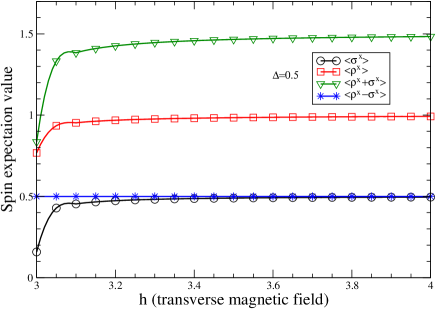
Figure 8: The magnetization of sublattices, the total magnetization, and the staggered magnetization per unit cell of an anisotropic ferrimagnetic spin-($1/2,1$) chain versus transverse field and for $\Delta=0.5$ and when the background in the linear SWT is the field-induced fully polarized state.

Again we consider the special case of ($\sigma=\frac{1}{2},\rho=1$) and $\Delta=0.5$. The Hamiltonian of this system in the linear SWT approximation is positive definite only for a magnetic field larger than $h^{SWT}_{c2}=3$. The magnetization of each sublattice, the total field-induced magnetization, and the staggered magnetization per unit cell are plotted in Fig. 8. For $h>3$, the model is in the polarized phase. We have already shown in Ref. Rezai 10 ; Abou 10 that the full saturation only happens for the isotropic case $\Delta=1$. Thus the model possesses an upper critical field $h_{c2}=3$ for $\Delta=1$. The comparison with DMRG results shows that $h^{SWT}_{c2}=3$ is the true value, which is the consequence of weak quantum fluctuations for the strong field regimes. For $\Delta\neq 1$, the fully saturated state appears at infinite magnetic field. It can be understood simply by imposing $\theta=0=\beta$ in Eq. (III.1) which can be fulfilled only for $\Delta=1$ in the Hamiltonian given by Eq. (1). In general, the full saturation occurs at a finite magnetic field if the model has the U(1) symmetry around the direction of the magnetic field.

Let us discuss qualitatively the effects of a non commuting transverse magnetic field on the phase diagram of the anisotropic ferrimagnetic spin-($1/2,1$) chain. The SWT gives two branches of quasi-particle excitations for each of the small, intermediate and large magnetic field regions. At zero magnetic field the lower branch is gapless with ferromagnetic nature while the upper one is gapped with antiferromagnetic signature. A nonzero magnetic field opens a gap in the ferromagnetic branch which remains robust for $h\leq h_{c1}$. Moreover, the staggered magnetization in the field direction is close to its maximum value which implies a Néel phase. At $h=h_{c1}$ a quantum phase transition from the Néel phase to the spin-flop phase takes place where the staggered magnetization perpendicular to the field direction becomes nonzero. The quasi-particle excitations for the spin-flop phase are given by $\omega^{\pm}(k)$. In the spin-flop phase ($h_{c1}<h<h_{c2}$) an entanglement phase transition occurs at $h=h_{f}$ where the quantum correlations become independent for $h<h_{f}$ and $h>h_{f}$. The increase of magnetic field causes the second quantum phase transition at $h=h_{c2}$ to a nearly polarized state in the field direction. The excitations in the field induced polarized phase ($h>h_{c2}$) are gapful given by $\Omega^{\pm}(k)$, where the gap is proportional to the magnetic field.

IV Summary and discussion

The ground state phase diagram of the anisotropic ferrimagnetic ($\sigma,\rho$) chain in the presence of a non commuting transverse magnetic field has been studied. The general picture has been obtained within the spin wave approximation. We have applied three schemes of linear spin wave approximation to find the magnetic phase diagram of the anisotropic ferrimagnetic spin-($\sigma,\rho$) chain with anisotropy parameter $\Delta$ and in the presence of the transverse magnetic field ($h$). The spin wave approximation has been applied close to $h=0$ (weak fields), $h=h_{f}$ (intermediate regime), and $h\gg h_{f}$ (strong fields), where $h_{f}$ is the factorizing magnetic field. The ground state is known exactly at $h=h_{f}$ as a product of single spin states. We have studied the magnetization in the field direction. There is a plateau at $M_{x}=0.5$ for isotropic case where the ground state energy is linear in magnetic field while no plateau observed for the anisotropic cases. However, the magnetization along the magnetic field changes slightly as long as $h\leq h_{c1}$ and its value is $M_{x}\simeq 0.5$, which motivates to recognize it as a Néel phase . The model exhibits a quantum phase transition at $h=h_{c1}$ from the Néel phase to (i) a spin-flop phase for $\Delta\neq 1$, (ii) a gapless Luttinger liquid for $\Delta=1$ Kolezhuk 99 ; Abolfath 01 . The magnetization evolves in the spin-flop phase when the magnetic field is increased. The spin-flop phase contains the factorizing field ($h=h_{f}$) where an entanglement phase transition takes place and quantum correlations vanish. Further increase of the magnetic field leads to a polarized phase which resembles a plateau at the saturated magnetization in the field direction. However, it will be fully saturated only for $\Delta=1$ (the presence of a rotational symmetry around the magnetic field) which is represented by a quantum phase transition at a finite value $h_{c2}$. The validity domain of spin wave analysis were introduced and it was shown that the corresponding results were in good agreement with the DMRG numerical computations.

To get more accurate values on the magnetization process of spin-($1/2,1$) ferrimagnet, we have also plotted in Fig. 9 the DMRG data of the $x$- and $y$-component staggered magnetization in addition to the $x$-component magnetization of unit cell versus the transverse magnetic field for $\Delta=0$. The magnetization curve has been divided to five regions which has been labeled in fig. 4, fig. 9, and also in Table. 1. Region-(1) is defined by the Néel phase for $0\leq h<h_{c1}\simeq 1.6$ where both $M_{x}$ and $SM_{x}$ are nearly constant while $SM_{y}$ is zero. The spin-flop (gapped) phase, $h_{c1}\leq h\leq h_{c2}$, where a nonzero $SM_{y}$ sets up can be distinguished to three parts, namely regions-(2-4). For $h_{c1}\leq h\lesssim 1.9$ which is labeled region-(2) we observe $\langle\sigma^{x}\rangle<0$ and $\langle\rho^{x}\rangle>0$. It is a spin-flop phase which is called spin-flop (I) in Table. 1. Region-(3) is defined at $h\simeq 1.9$ where the projection of smaller spin along the magnetic field becomes zero, $\langle\sigma^{x}\rangle=0$, i.e. $M_{x}=SM_{x}$. The rest, $1.9\lesssim h\leq h_{c2}\simeq 2.4$, labeled by region-(4) where $\langle\sigma^{x}\rangle>0$ and $\langle\rho^{x}\rangle>0$ is called spin-flop (II). The region-(5) is the polarized phase along the direction of magnetic field, i.e. $M_{x}\simeq 1.5$ and $SM_{y}=0$. It is observed from Fig. 2-(a) that the component of smaller spin in the direction of the magnetic field is affected strongly by the magnetic field while the corresponding component for the larger one is almost constant.

The spin-flop (I) is a characteristic behavior of XXZ ferrimagnets in the presence of transverse magnetic field because the spin component of the smaller spin along the magnetic field is opposite to the field direction ($\langle\sigma^{x}\rangle<0$) while the spin-flop (II) is similar to the corresponding phase of the homogeneous XXZ spin chain in the presence of transverse magnetic field ($\langle\sigma^{x}\rangle>0$) Langari 04 ; Abou 10 . In the anisotropic ferrimagnetic chain the transverse field first develops a Néel phase and a field-induced quantum phase transition leads to a spin-flop phase. Moreover, the Z₂ symmetry is spontaneously broken for small-field region in the homogeneous spin chain while it will be broken in the intermediate fields $h_{c1}(\Delta)<h<h_{c2}(\Delta)$ for ferrimagnets. A summary of different properties of the homogenous XXZ spin 1/2 chain and the corresponding ($1/2,1$) ferrimagnet both for isotropic and anisotropic cases is presented in Table. 2.

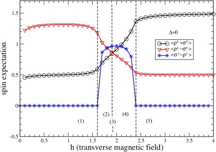
Figure 9: The $x$-component magnetization, $x$- and $y$-components staggered magnetization versus the transverse field for a ferrimagnetic spin-($1/2,1$) chain. Effects of the magnetic field on the spins of each sublattice are divided into five different regions.

Table 1: Different configurations of the ground state of the ferrimagnetic spin-($1/2,1$) chain with $\Delta=0$ in the presence of a transverse magnetic field.

Region	$h$	Phase	Order parameters
(1)	$0\leq h<1.6$	Néel	$M_{x}=1/2,SM_{y}=0$
(2)	$1.6\leq h<1.9$	Spin-Flop(I)	$\langle\sigma^{x}\rangle<0,SM_{y}>0$
(3)	$h\simeq 1.9$	Spin-Flop	$\langle\sigma^{x}\rangle=0,SM_{y}>0$
(4)	$1.9\leq h<2.4$	Spin-Flop(II)	$\langle\sigma^{x}\rangle>0,SM_{y}>0$
(5)	$h>2.4$	Nearly Polarized	$M_{x}\simeq 3/2,SM_{y}=0$

It is also interesting to mention that the low energy effective Hamiltonian of the anisotropic spin-($1/2,1$) chain in the presence of a transverse magnetic field can be represented by the fully anisotropic (XYZ) spin-1/2 Heisenberg chain in an applied field (though we do not report such calculations in this paper). This helps to get more knowledge from the results on the effective model 0208216 . However, both spin wave approximation and DMRG results show that the model has two nearly constant magnetization in the presence of transverse magnetic field, the small-field plateau at $M_{x}\simeq 0.5$ for $h<h_{c1}(\Delta)$ and the saturated $M_{x}\simeq 1.5$ for large fields ($h>h_{c2}(\Delta)$). The general behavior is the same for any value of the anisotropy parameter ($\Delta$); however, the critical fields $h_{c1}(\Delta)$ and $h_{c2}(\Delta)$ depend on $\Delta$. For instance, $h_{c1}(\Delta=0.5)\simeq 1.8$ and $h_{c2}(\Delta=0.5)\simeq 2.6$.

Table 2: Different ground state phases are classified for the heterogeneous spin-($1/2,1$) XXZ ferrimagnet along with the homogeneous spin $1/2$ XXZ antiferromagnet. The comparision between isotropic and anisotropic cases in the presence of the transverse magnetic field ($h$) is presented. The magnetization per unit cell is $m$. The ferrimagnet has two critical points $h_{c1}$ and $h_{c2}$ while the homogeneous antiferromagnet has a critical point at $h_{c}$.

Spin	Region	Isotropic case ($\Delta=1$)	Anisotropic case ($\Delta\neq 1$)
($1/2,1$)	$0\leq h<h_{c1}$	Gapped Néel, plateau at $m=1/2$	Gapped Néel, no plateau
($1/2,1$)	$h_{c1}<h<h_{c2}$	Gapless Luttinger liquid, no plateau	Gapped spin-flop, no plateau
($1/2,1$)	$h>h_{c2}$	Gapped paramagnet, plateau at $m=3/2$	Gapped paramagnet, no plateau
$1/2$	$0\leq h<h_{c}$	Gapless spin-fluid, no plateau	Gapped spin-flop, no plateau
$1/2$	$h>h_{c}$	Gapped paramagnet, plateau at $m=1/2$	Gapped paramagnet, no plateau

The magnetization process can also be viewed as a non-unitary evolution of the system. The entanglement of a pure state (ground state in our case) is conserved under local unitary operations Bennett 96 . For the ferrimagnetic spin-($1/2,1$) chain, the entanglement of the system is decreased by increasing the magnetic field for $h<h_{f}$. The entanglement vanishes at $h=h_{f}$ where the ground state is given by a tensor product state. This is an entanglement phase transition. It is thus concluded that the effect of magnetic field is a non-unitary evolution of the ground state.

V acknowledgment

J.A thanks H. Movahhedian for his fruitful comments. A. L. would like to thank A. T. Rezakhani for his detailed comments on the final version of the manuscript. A.L and M.R. would like to thank the hospitality of physics department of the institute for research in fundamental sciences (IPM) during part of this collaboration. This work was supported in part by the Center of Excellence in Complex Systems and Condensed Matter (www.cscm.ir). The DMRG computation has been done by using ALPS package ALPS which is acknowledged.

References

References

- (1) Gleizes A and Verdaguer M, Ordered magnetic bimetallic chains: a novel class of one-dimensional compounds, 1981 J. Am. Chem. Soc. 103, 7373; Gleizes A and Verdaguer M, Additions and Corrections - Structurally Ordered Bimetallic One-Dimensional catena--Dithiooxalato Compounds: Synthesis, Crystal and Molecular Structures, and Magnetic Properties of AMn(S2C2O2)2(H2O)4.5H2O (A = Cu, Ni, Pd, Pt), 1984 J. Am. Chem. Soc. 106, 3727
- (2) Pei Y, Verdaguer M, Kahn O, Sletten J and Renard J.-P Magnetism of manganese(II)copper(II) and nickel(II)copper(II) ordered bimetallic chains. Crystal structure of MnCu(pba)(H2O)3.2H2O (pba = 1,3-propylenebis(oxamato)), 1987 Inorg. Chem. 26, 138; Kahn O, Pei Y, Verdaguer M, Renard J.-P and Sletten J, Magnetic ordering of manganese(II) copper(II), bimetallic chains; design of a molecular based ferromagnet, 1988 J. Am. Chem. Soc. 110, 782; J. van Koningsbruggen P, Kahn O, Nakatani K, Pei Y and Renard J.-P, Magnetism of A-copper(II) bimetallic chain compounds (A = iron, cobalt, nickel): one- and three-dimensional behaviors, 1990 Inorg. Chem. 29, 3325
- (3) Pati S. K, Ramasesha S and Sen D, Low-lying excited states and low-temperature properties of an alternating spin-1 spin-1/2 chain: A density-matrix renormalization-group study, 1997 Phys. Rev. B 55, 8894
- (4) Yamamoto S, Magnetic properties of quantum ferrimagnetic spin chains, 1999 Phys. Rev. B 59, 1024
- (5) Kolezhuk A. K, Mikeska H.-J, Maisinger K and Schollwöck U, Spinon signatures in the critical phase of the (1,1/2) ferrimagnet in a magnetic field, 1999 Phys. Rev. B 59, 13565
- (6) Abouie J and Langari A, Cumulant expansion for ferrimagnetic spin (S1,s2) systems, 2004 Phys. Rev. B 70, 184416; Abouie J and Langari A, Thermodynamic properties of ferrimagnetic large spin systems, 2005 J. Phys.: Condens. Matter 17, S1293
- (7) Abouie J, Ghasemi A and Langari A, Thermodynamic properties of ferrimagnetic spin chains in the presence of a magnetic field, 2006 Phys. Rev. B 73, 14411
- (8) Yamamoto S, Brehmer S and Mikeska H.-J, Elementary excitations of Heisenberg ferrimagnetic spin chains, 1998 Phys. Rev. B 57, 13610
- (9) Langari A, Abolfath M and Martin-Delgado M. A, Phase diagram of ferrimagnetic ladders with bond alternation, 2000 Phys. Rev. B 61, 343
- (10) Langari A and Martin-Delgado M. A, Low-energy properties of ferrimagnetic two-leg ladders: A Lanczos study, 2001 Phys. Rev. B 63, 54432
- (11) Alcaraz F. C and Malvezzi A. L, Critical behaviour of mixed Heisenberg chains, 1997 J. Phys. A: Math. Gen 30, 767
- (12) Sakai T, Yamamoto S, Critical behavior of anisotropic Heisenberg mixed-spin chains in a field, 1999 Phys. Rev. B 60, 4053
- (13) Abolfath M and Langari A, Superfluid spiral state of quantum ferrimagnets in a magnetic field, 2001 Phys. Rev. B 63, 144414
- (14) Langari A and Martin-Delgado M. A, Alternating-spin ladders in a magnetic field: Formation of magnetization plateaux, 2000 Phys. Rev. B 62, 11725
- (15) Oshikawa M, Yamanaka M and Affleck I, Magnetization Plateaus in Spin Chains: Haldane Gap for Half-Integer Spins, 1997 Phys. Rev. Lett. 78, 1984
- (16) Dmitriev D. V, Krivnov V. Y, Ovchinnikov A. A and Langari A, One-dimensional anisotropic Heisenberg model in the transverse magnetic field, 2002 JETP 95, 538
- (17) Caux J-S, Essler F. H. L, and Löw U Dynamical structure factor of the anisotropic Heisenberg chain in a transverse field, 2003 Phys. Rev. B 68, 134431
- (18) Langari A, Quantum renormalization group of XYZ model in a transverse magnetic field, 2004 Phys. Rev. B 69, 100402(R)
- (19) Dmitriev D. V and Krivnov V. Y, Anisotropic Heisenberg chain in coexisting transverse and longitudinal magnetic fields, 2004 Phys. Rev. B. 70, 144414
- (20) Langari A and Mahdavifar S, Gap exponent of the XXZ model in a transverse field, 2006 Phys. Rev. B. 73, 054410
- (21) Oshikawa M, Commensurability, excitation gap, and topology in quantum many-body systems on a periodic lattice, 2000 Phys. Rev. Lett. 84, 1535
- (22) White S. R, Density-matrix algorithms for quantum renormalization groups, 1993 Phys. Rev. B 48, 10345
- (23) Rezai M, Langari A and Abouie J, Factorized ground state for a general class of ferrimagnets, 2010 Phys. Rev. B 81, 060401(R)
- (24) Siahatgar M and Langari A, Thermodynamic properties of the XXZ model in a transverse field, 2008 Phys. Rev. B 77 054435
- (25) Abouie J, Langari A and Siahatgar M, Thermodynamic behavior of the XXZ Heisenberg s = 1/2 chain around the factorizing magnetic field, 2010 J. Phys. :Condens. Matter 22, 216008
- (26) Colpa J. H. P, Diagonalization of the quadratic boson hamiltonian, 1978 Physica A 93, 327
- (27) Dutta A and Sen D, Gapless line for the anisotropic Heisenberg spin-1/2 chain in a magnetic field and the quantum axial next-nearest-neighbor Ising chain, 2003 Phys. Rev. B 67, 094435
- (28) Bennett C. H, DiVincenzo D. P, Smolin J. A and Wootters W. K, Mixed-state entanglement and quantum error correction, 1996 Phys. Rev. A 54, 3824
- (29) Albuquerque F et. al, The ALPS project release 1.3: Open-source software for strongly correlated systems, 2007 Journal of Magnetism and Magnetic Materials 310, 1187