Two loop renormalization of the $n$ $=$ $2$ Wilson operator in the RI^′/SMOM scheme

Abstract. We compute the anomalous dimensions of the flavour non-singlet twist-$2$ Wilson operators in the RI^′/SMOM scheme at two loops in an arbitrary linear covariant gauge. In addition we provide the full Green’s function for these operators inserted in a quark $2$-point function at the symmetric subtraction point. The three loop anomalous dimensions in the Landau gauge are also derived.

LTH 910

1 Introduction.

In a quantum field theory the behaviour of the Green’s functions or $n$-point functions derived from the Lagrangian carry all the information about the dynamics of the quantum particles. For the vast majority of quantum field theories, however, it is impossible to extract their behaviour for all ranges of momenta and parameters, such as the particle masses and coupling constants. Instead one invariably examines them in various regions of interest, such as at high or low energy, using a variety of techniques. For instance, at high energy in Quantum Chromodynamics (QCD) one uses perturbation theory since the coupling constant is small as a consequence of asymptotic freedom, [1, 2]. By contrast at low energy perturbation theory breaks down and non-perturbative methods have been developed and refined to give credible information. The central tool at this energy is lattice gauge theory involving an intense amount of numerical computations on high performance computers. This approach has in general been hugely successful in determining bound state masses, for example, and exploring the structure of nucleons. For instance, matrix elements of the underlying operators used in deep inelastic scattering, known as Wilson operators, play a key role in this, [3]. The behaviour of such matrix elements at low energy is useful in extracting theoretical information for parton structure functions. In outlining the general aspects of Green’s functions in understanding the dynamics of the strong nuclear force, we are overlooking the huge technical effort which is required to ensure accurate estimates are obtained. For instance, as one is dealing with a quantum field theory, the operators undergo renormalization, [3]. Equally when one produces estimates from a low energy computation on the lattice one has to be assured that the result is consistent with and extrapolates onto the high energy behaviour of the same object which can be computed within perturbation theory. Indeed there has been a large degree of activity on the lattice in this respect for quark currents and Wilson operators. For instance, see [4, 5, 6, 7, 8, 9, 10, 11, 12, 13, 14, 15, 16, 17, 18, 19, 20] for representative analyses.

For the continuum computations one usually calculates in the $\overline{\mbox{MS}}$ scheme which is a mass independent renormalization scheme. The advantage of this scheme is that it is one in which the largest order of perturbation theory can be determined. However, defining the same scheme for lattice calculations is not as easy since it invariably requires a numerical differentiation on the lattice. Taking such derivatives carries a financial penalty. Therefore, alternative schemes have been developed for lattice gauge theory which avoids the use of derivatives. Such a class of schemes is generally referred to as Regularization Invariant (RI), [21, 22]. However, there are two main types. The original class involves RI itself and a modified version known as RI^′, [21, 22]. These are similar in that QCD is renormalized for $3$-point and higher Green’s functions according to the $\overline{\mbox{MS}}$ prescription but for $2$-point functions such as those determining propagator corrections, the renormalization condition is defined by ensuring that the contributions from radiative corrections at the subtraction point are absent. In this class of schemes we include the zero momentum insertion of an operator in, say, a quark $2$-point function. The modified scheme, RI^′, differs from RI in the way the quark wave function is defined, [21, 22]. Whilst originally defined in [21, 22] specifically in the context of the lattice, this scheme has also been studied in the Landau gauge in the continuum at three and four loops, [23], and at three loops in an arbitrary linear covariant gauge, [24]. Subsequently, the Green’s functions of a variety of low moment twist-$2$ flavour non-singlet operators central to deep inelastic scattering inserted in a quark $2$-point function were evaluated to three loops in $\overline{\mbox{MS}}$ and RI^′, [25, 26]. This high order of perturbation theory provided useful information on matching the lattice measurement of the same object at high energy.

More recently a second class of regularization invariant schemes has been developed in [27, 28, 29]. It is termed RI^′/SMOM where the first part of the designation indicates the RI^′ scheme definition of the quark wave function renormalization. The second refers to the method used to define the renormalization constants of $3$-point functions with an operator insertion at non-zero momentum. As there are momenta flowing into each point of the Green’s function, the renormalization is carried out at a symmetric point where the squared momenta of all three incoming momenta take the same value which is the origin of the S. The MOM indicates the ethos that was present in the overall RI definition in that the condition for defining the operator renormalization constant is to ensure that the part corresponding to radiative corrections at this symmetric subtraction point are absent. This particular scheme was developed to avoid the strong sensitivity of the RI^′ scheme to infrared effects, [27], as well as to try and have a more rapidly convergent perturbation series for the conversion functions to the $\overline{\mbox{MS}}$ scheme. It was initially applied to the renormalization of the quark currents at one loop in [27] to determine the anomalous dimensions, amplitudes and conversion functions in the $\overline{\mbox{MS}}$ scheme. Subsequently, the two loop renormalization of the scalar and tensor currents was treated in [28, 29] with the anomalous dimensions and conversion functions being computed. Though with the knowledge of the two loop conversion functions the three loop Landau gauge anomalous dimensions were deduced too. More recently, the full set of amplitudes for the scalar, vector and tensor currents have been calculated at two loops in [30].

Given that the measurement of nucleon matrix elements is of interest it is the purpose of this article to provide the anomalous dimensions and amplitudes for the second moment of the flavour non-singlet Wilson operator at two loops in RI^′/SMOM. This will build on the analogous one loop computation of [31]. The treatment of this operator is complicated by the fact that it mixes with a total derivative operator. Ordinarily one is not concerned by this extra operator since if it were inserted at zero momentum it would give no contribution to the Green’s function. However, the symmetric subtraction point of the RI^′/SMOM scheme means that such total derivative operators play an active role and cannot be ignored. The full three loop $\overline{\mbox{MS}}$ mixing matrix of anomalous dimensions for this second moment operator was given in [32]. With the two loop conversion functions we will provide the three loop result in the RI^′/SMOM scheme. One feature of the RI^′/SMOM construction for the Wilson operators is the role the vector current has in the renormalization. Its relation to the Slavnov-Taylor identity was discussed in [27] at one loop, as well as two loop, [30], and in the context of the Wilson operators in [31]. The divergence of the vector current resides within the total derivative operator into which the Wilson operator mixes. Hence, the two loop renormalization of the vector current and the associated RI^′/SMOM amplitudes of the Green’s function where this was determined, [30], are important as checks on the computation presented here. Indeed partly related to this is that one has to ensure the renormalization of the second moment is consistent with one of the Slavnov-Taylor identities of QCD. Further, the third moment of the Wilson operator was also considered at one loop in [31]. From that it transpires that the renormalization of the higher moment operators is dependent on that of the lower moment operators of the tower with the vector current at the foundation. Therefore, the treatment of the $n$ $=$ $2$ moment is relevant for that of the higher moment operators. Throughout we will use $N_{\!f}$ flavours of massless quarks and therefore all our expressions are in the chiral limit. Including masses for quarks is not currently viable as the basic scalar master Feynman integrals have not been evaluated for the momentum configuration of the Green’s function we consider here.

The article is organized as follows. The background to the formalism we will use, notation and method to define and extract the scalar amplitudes of interest are discussed in section two. Section three is devoted to summarizing the main results of the RI^′/SMOM computation of the second moment of the Wilson operator. The amplitudes are given numerically. Though the full exact expressions are recorded in the form of a set of tables. The results relating to the actual operator renormalization, such as the anomalous dimensions and conversion functions are provided in section four whilst we summarize our conclusions in section five.

2 Preliminaries.

First, we recall the key properties of the operators we will consider. We use the notation of [32] in this respect and denote

$$W_{2}~{}\equiv~{}{\cal S}\bar{\psi}\gamma^{\mu}D^{\nu}\psi~{}~{}~{},~{}~{}~{}\partial W_{2}~{}\equiv~{}{\cal S}\partial^{\mu}\left(\bar{\psi}\gamma^{\nu}\psi\right)$$ (2.1)

where $D_{\mu}$ is the covariant derivative with all derivatives acting to the right and ${\cal S}$ indicates that the operator is traceless and symmetric in its Lorentz indices. Moreover, as we will be using dimensional regularization we regard the operators as being traceless in $d$-dimensions. So, for instance, we have

$${\cal S}{\cal O}^{W_{2}}_{\mu\nu}~{}=~{}{\cal O}^{W_{2}}_{\mu\nu}~{}+~{}{\cal O}^{W_{2}}_{\nu\mu}~{}-~{}\frac{2}{d}\eta_{\mu\nu}{\cal O}^{W_{2}\,\sigma}_{\sigma}$$ (2.2)

where

$${\cal O}^{W_{2}}_{\mu\nu}~{}=~{}\bar{\psi}\gamma_{\mu}D_{\nu}\psi~{}.$$ (2.3)

The total derivative operator denoted by $\partial W_{2}$ also obeys the same symmetrization. Throughout we concentrate on flavour non-singlet operators and omit the flavour indices on the quark fields $\psi$. Ordinarily when one renormalizes $W_{2}$ in perturbation theory the operator is inserted in a quark $2$-point function, [3, 33, 34], at zero momentum. Then the renormalization constant emerges under the assumption that the renormalization of this operator is multiplicative. This is not strictly speaking true. It is only true for that particular momentum routing through the quark $2$-point Green’s function with the operator insertion. If instead there was a momentum flowing out through the operator then there is a mixing with the total derivative operator. The Feynman rule for the latter operator vanishes when there is no momentum flow out through the operator which is why the momentum configuration of [3, 33, 34] is multiplicative. In other words for the full renormalization of $W_{2}$ one has to determine the mixing matrix of renormalization constants where $\partial W_{2}$ completes the set. As we are considering the renormalization of $W_{2}$ in the RI^′/SMOM scheme we have to take this into account as the momentum setup for the underlying Green’s function involves two independent momenta flowing in through the external quark legs and out through the operator itself. This is illustrated in Figure $1$.

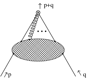
Figure 1: The Green’s function $\left\langle\psi(p){\cal O}^{i}_{\mu_{1}\ldots\mu_{n_{i}}}(-p-q)\bar{\psi}(q)\right\rangle$.

The renormalization of the set of level $W_{2}$ operators has been carried out to three loops in the $\overline{\mbox{MS}}$ scheme in [32]. As we will require these later for the three loop RI^′/SMOM scheme anomalous dimensions later we briefly recall the relevant results and formalism. First, irrespective of which scheme one works in the mixing matrix of renormalization constants is

$$Z^{W_{2}}_{ij}~{}=~{}\left(\begin{array}[]{cc}Z^{W_{2}}_{11}&Z^{W_{2}}_{12}\\ 0&Z^{W_{2}}_{22}\\ \end{array}\right)~{}.$$ (2.4)

Here we retain the notation of [31, 32] whereby the superscript indicates the operator level $W_{2}$ and the labels indicating the matrix elements respectively label the two elements of the operators in that set which are $W_{2}$ and $\partial W_{2}$. Whilst $W_{2}$ is used to mean level and operator it will be clear from the context which is meant. The anomalous dimensions are formally defined by

$$\gamma^{W_{2}}_{ij}(a,\alpha)~{}=~{}-~{}\mu\frac{d~{}}{d\mu}\ln Z^{W_{2}}_{ij}$$ (2.5)

where here and below $W_{2}$ represents the level, from which one can deduce the relations between the individual matrix elements are

$$0 = \gamma^{W_{2}}_{11}(a,\alpha)Z^{W_{2}}_{11}~{}+~{}\mu\frac{d~{}}{d\mu}Z^{W_{2}}_{11}$$

$$0 = \gamma^{W_{2}}_{11}(a,\alpha)Z^{W_{2}}_{12}~{}+~{}\gamma^{W_{2}}_{12}(a,\alpha)Z^{W_{2}}_{22}~{}+~{}\mu\frac{d~{}}{d\mu}Z^{W_{2}}_{12}$$

$$0 = \gamma^{W_{2}}_{22}(a,\alpha)Z^{W_{2}}_{22}~{}+~{}\mu\frac{d~{}}{d\mu}Z^{W_{2}}_{22}$$ (2.6)

with

$$\mu\frac{d~{}}{d\mu}~{}=~{}\beta(a)\frac{\partial~{}}{\partial a}~{}+~{}\alpha\gamma_{\alpha}(a,\alpha)\frac{\partial~{}}{\partial\alpha}$$ (2.7)

and $\gamma_{\alpha}(a,\alpha)$ is the anomalous dimension of the gauge parameter. We retain our previous conventions, [31, 32], for consistency. In the $\overline{\mbox{MS}}$ scheme since the operators $W_{2}$ and $\partial W_{2}$ are gauge invariant then the anomalous dimensions are independent of the gauge parameter. However, for mass dependent renormalization schemes, of which RI^′/SMOM is an example, the anomalous dimensions are $\alpha$ dependent. Therefore, we recall that for the $\overline{\mbox{MS}}$ scheme

$$\left.\frac{}{}\gamma^{W_{2}}_{11}(a)\right|_{\overline{\mbox{\footnotesize{MS}}}} = \frac{8}{3}C_{F}a~{}+~{}\frac{1}{27}\left[376C_{A}C_{F}-112C_{F}^{2}-128C_{F}T_{F}N_{\!f}\right]a^{2}$$

$$+~{}\frac{1}{243}\left[\left(5184\zeta(3)+20920\right)C_{A}^{2}C_{F}-\left(15552\zeta(3)+8528\right)C_{A}C_{F}^{2}\right.$$

$$\left.~{}~{}~{}~{}~{}~{}~{}~{}~{}~{}-~{}\left(10368\zeta(3)+6256\right)C_{A}C_{F}T_{F}N_{\!f}+\left(10368\zeta(3)-560\right)C_{F}^{3}\right.$$

$$\left.~{}~{}~{}~{}~{}~{}~{}~{}~{}~{}+~{}\left(10368\zeta(3)-6824\right)C_{F}^{2}T_{F}N_{\!f}-896C_{F}T_{F}^{2}N_{\!f}^{2}\right]a^{3}~{}+~{}O(a^{4})$$

$$\left.\frac{}{}\gamma^{W_{2}}_{12}(a)\right|_{\overline{\mbox{\footnotesize{MS}}}} = -~{}\frac{4}{3}C_{F}a~{}+~{}\frac{1}{27}\left[56C_{F}^{2}-188C_{A}C_{F}+64C_{F}T_{F}N_{\!f}\right]a^{2}$$

$$+~{}\frac{1}{243}\left[\left(7776\zeta(3)+4264\right)C_{A}C_{F}^{2}-\left(2592\zeta(3)+10460\right)C_{A}^{2}C_{F}\right.$$

$$\left.~{}~{}~{}~{}~{}~{}~{}~{}~{}~{}+~{}\left(5184\zeta(3)+3128\right)C_{A}C_{F}T_{F}N_{\!f}-\left(5184\zeta(3)-280\right)C_{F}^{3}\right.$$

$$\left.~{}~{}~{}~{}~{}~{}~{}~{}~{}~{}-~{}\left(5184\zeta(3)-3412\right)C_{F}^{2}T_{F}N_{\!f}+448C_{F}T_{F}^{2}N_{\!f}^{2}\right]a^{3}~{}+~{}O(a^{4})$$

$$\left.\frac{}{}\gamma^{W_{2}}_{22}(a)\right|_{\overline{\mbox{\footnotesize{MS}}}} = O(a^{4})$$ (2.8)

where $\zeta(z)$ is the Riemann zeta function and for this scheme we have omitted the part of the argument involving $\alpha$ to emphasise the absence of gauge dependence. The colour group Casimirs are defined by

$$T^{a}T^{a}~{}=~{}C_{F}~{}~{}~{},~{}~{}~{}f^{acd}f^{bcd}~{}=~{}C_{A}\delta^{ab}~{}~{}~{},~{}~{}~{}\mbox{Tr}\left(T^{a}T^{b}\right)~{}=~{}T_{F}\delta^{ab}$$ (2.9)

where $T^{a}$ are the colour group generators with structure constants $f^{abc}$ and $1$ $\leq$ $a$ $\leq$ $N_{A}$ with $N_{A}$ the dimension of the adjoint representation. The coupling constant appearing in the covariant derivative is $g$ but appears in (2.8) in the combination $a$ $=$ $g^{2}/(16\pi^{2})$. The absence of a correction to $\left.\!\!\!\frac{}{}\gamma^{W_{2}}_{22}(a)\right|_{\overline{\mbox{\footnotesize{MS}}}}$ to this order is a reflection of the all orders result where there is no renormalization of $\partial W_{2}$. This is because it corresponds to the vector current which is a physical operator and is not renormalized reflecting the Slavnov-Taylor identity of the underlying gauge theory. See, for example, [35] for background. Moreover, this property is retained in all schemes and we must ensure that the RI^′/SMOM scheme renormalization respects this general feature.

In order to define the RI^′/SMOM renormalization scheme for level $W_{2}$ we compute the Green’s function illustrated in Figure $1$ where the external momenta $p$ and $q$ are independent. However, we will focus totally on its structure at the symmetric subtraction point, [27], which is defined as

$$p^{2}~{}=~{}q^{2}~{}=~{}(p+q)^{2}~{}=~{}-~{}\mu^{2}$$ (2.10)

where $\mu$ is the common mass scale. These relations imply

$$pq~{}=~{}\frac{1}{2}\mu^{2}~{}.$$ (2.11)

In order to determine the renormalization constant in the $\overline{\mbox{MS}}$ or RI^′ schemes one can proceed with only one external momentum. For instance, the choice $p$ $=$ $-$ $q$ corresponds to a zero momentum insertion before setting $p^{2}$ to be a specific scale involving $\mu^{2}$. Though in fact to determine the full mixing matrix in the $\overline{\mbox{MS}}$ scheme requires accessing the total derivative operators which is achieved by nullifiying the momentum of one of the external quark legs, [32]. As the operators we consider have free Lorentz indices then the Green’s function has to be decomposed into a set of Lorentz invariant amplitudes. The basis for $W_{2}$ has already been constructed in [31] and we briefly recall the construction as well as the notation. First, we write the Green’s function as

$$\left.\left\langle\psi(p){\cal O}^{i}_{\mu_{1}\ldots\mu_{n_{i}}}(-p-q)\bar{\psi}(q)\right\rangle\right|_{p^{2}=q^{2}=-\mu^{2}}~{}=~{}\sum_{k=1}^{n_{i}}{\cal P}^{i}_{(k)\,\mu_{1}\ldots\mu_{n_{i}}}(p,q)\,\Sigma^{{\cal O}^{i}}_{(k)}(p,q)~{}.$$ (2.12)

Here $\Sigma^{{\cal O}^{i}}_{(k)}(p,q)$ are the scalar amplitudes for each of the two operators ${\cal O}^{i}$ whereas ${\cal P}^{i}_{(k)\,\mu_{1}\ldots\mu_{n_{i}}}(p,q)$ are the Lorentz tensors of the basis whose Lorentz indices reflect the symmetries of the operator which has been inserted. For level $W_{2}$ there are ten independent Lorentz tensors and we will detail these later. To evaluate the scalar amplitudes we use the method of projection where we apply different linear combinations of the basis tensors to the Green’s function in such a way that each amplitude is isolated in turn. More specifically we have, [32],

$$\Sigma^{{\cal O}^{i}}_{(k)}(p,q)~{}=~{}{\cal M}^{i}_{kl}{\cal P}^{i~{}\,\mu_{1}\ldots\mu_{n_{i}}}_{(l)}(p,q)\left.\left(\left\langle\psi(p){\cal O}^{i}_{\mu_{1}\ldots\mu_{n_{i}}}(-p-q)\bar{\psi}(q)\right\rangle\right)\right|_{p^{2}=q^{2}=-\mu^{2}}$$ (2.13)

where ${\cal M}^{i}_{kl}$ is a matrix of rational polynomials in the spacetime dimension $d$. It is constructed by first determining the matrix ${\cal N}^{i}_{kl}$ which is defined by the contraction of the tensors of the basis with each of the other tensors via

$${\cal N}^{i}_{kl}~{}=~{}\left.{\cal P}^{i}_{(k)\,\mu_{1}\ldots\mu_{n_{i}}}(p,q){\cal P}^{i~{}\,\mu_{1}\ldots\mu_{n_{i}}}_{(l)}(p,q)\right|_{p^{2}=q^{2}=-\mu^{2}}~{}.$$ (2.14)

Then ${\cal M}^{i}_{kl}$ is the inverse of ${\cal N}^{i}_{kl}$.

More specifically, the basis of Lorentz tensors into which we decompose the Green’s functions with the operator insertions is, [32],

$${\cal P}^{W_{2}}_{(1)\mu\nu}(p,q) = \gamma_{\mu}p_{\nu}+\gamma_{\nu}p_{\mu}-\frac{2}{d}p\!\!\!/\eta_{\mu\nu}~{}~{},~{}~{}{\cal P}^{W_{2}}_{(2)\mu\nu}(p,q)~{}=~{}\gamma_{\mu}q_{\nu}+\gamma_{\nu}q_{\mu}-\frac{2}{d}q\!\!\!/\eta_{\mu\nu}$$

$${\cal P}^{W_{2}}_{(3)\mu\nu}(p,q) = p\!\!\!/\left[\frac{1}{\mu^{2}}p_{\mu}p_{\nu}+\frac{1}{d}\eta_{\mu\nu}\right]~{}~{},~{}~{}{\cal P}^{W_{2}}_{(4)\mu\nu}(p,q)~{}=~{}p\!\!\!/\left[\frac{1}{\mu^{2}}p_{\mu}q_{\nu}+\frac{1}{\mu^{2}}q_{\mu}p_{\nu}-\frac{1}{d}\eta_{\mu\nu}\right]$$

$${\cal P}^{W_{2}}_{(5)\mu\nu}(p,q) = p\!\!\!/\left[\frac{1}{\mu^{2}}q_{\mu}q_{\nu}+\frac{1}{d}\eta_{\mu\nu}\right]~{}~{},~{}~{}{\cal P}^{W_{2}}_{(6)\mu\nu}(p,q)~{}=~{}q\!\!\!/\left[\frac{1}{\mu^{2}}p_{\mu}p_{\nu}+\frac{1}{d}\eta_{\mu\nu}\right]$$

$${\cal P}^{W_{2}}_{(7)\mu\nu}(p,q) = q\!\!\!/\left[\frac{1}{\mu^{2}}p_{\mu}q_{\nu}+\frac{1}{\mu^{2}}q_{\mu}p_{\nu}-\frac{1}{d}\eta_{\mu\nu}\right]~{},~{}{\cal P}^{W_{2}}_{(8)\mu\nu}(p,q)~{}=~{}q\!\!\!/\left[\frac{1}{\mu^{2}}q_{\mu}q_{\nu}+\frac{1}{d}\eta_{\mu\nu}\right]$$

$${\cal P}^{W_{2}}_{(9)\mu\nu}(p,q) = \frac{1}{\mu^{2}}\left[\Gamma_{(3)\,\mu pq}p_{\nu}+\Gamma_{(3)\,\nu pq}p_{\mu}\right]$$

$${\cal P}^{W_{2}}_{(10)\mu\nu}(p,q) = \frac{1}{\mu^{2}}\left[\Gamma_{(3)\,\mu pq}q_{\nu}+\Gamma_{(3)\,\nu pq}q_{\mu}\right]~{}.$$ (2.15)

As there are ten elements in the basis then in order to save space for presenting the projection matrix, we have partitioned the $10$ $\times$ $10$ matrix into four sub-matrices. Defining

$${\cal M}^{W_{2}} = -~{}\frac{1}{108(d-2)}\left(\begin{array}[]{cc}{\cal M}^{W_{2}}_{11}&{\cal M}^{W_{2}}_{12}\\ {\cal M}^{W_{2}}_{21}&{\cal M}^{W_{2}}_{22}\\ \end{array}\right)$$ (2.18)

then we have

$${\cal M}^{W_{2}}_{11} = \left(\begin{array}[]{ccccc}18&9&48&24&12\\ 9&18&24&30&24\\ 48&24&64(d+1)&32(d+1)&16(d+4)\\ 24&30&32(d+1)&8(5d-1)&8(4d+1)\\ 12&24&16(d+4)&8(4d+1)&32(2d-1)\\ \end{array}\right)~{},$$ (2.24)

$${\cal M}^{W_{2}}_{12} = \left(\begin{array}[]{ccccc}24&30&24&0&0\\ 12&24&48&0&0\\ 32(d+1)&16(d+4)&8(d+10)&0&0\\ 16(d+1)&20(d+1)&16(d+4)&0&0\\ 8(d+4)&16(d+1)&32(d+1)&0&0\\ \end{array}\right)~{},$$ (2.30)

$${\cal M}^{W_{2}}_{21} = \left(\begin{array}[]{ccccc}24&12&32(d+1)&16(d+1)&8(d+4)\\ 30&24&16(d+4)&20(d+1)&16(d+1)\\ 24&48&8(d+10)&16(d+4)&32(d+1)\\ 0&0&0&0&0\\ 0&0&0&0&0\\ \end{array}\right)~{},$$ (2.36)

$${\cal M}^{W_{2}}_{22} = \left(\begin{array}[]{ccccc}32(2d-1)&8(4d+1)&16(d+4)&0&0\\ 8(4d+1)&8(5d-1)&32(d+1)&0&0\\ 16(d+4)&32(d+1)&64(d+1)&0&0\\ 0&0&0&-24&-12\\ 0&0&0&-12&-24\\ \end{array}\right)~{}.$$ (2.42)

We note that here the label $W_{2}$ refers to the level and the same projection is used for $\partial W_{2}$. In defining this basis we have used the set of generalized $\gamma$-matrices denoted by $\Gamma_{(n)}^{\mu_{1}\ldots\mu_{n}}$ which are totally antisymmetric in the Lorentz indices and defined by, [36, 37, 38],

$$\Gamma_{(n)}^{\mu_{1}\ldots\mu_{n}}~{}=~{}\gamma^{[\mu_{1}}\ldots\gamma^{\mu_{n}]}$$ (2.43)

where the notation includes the overall factor of $1/n!$. For simplicity we will retain the more natural notation for a single $\gamma$-matrix rather than use the clumsy $\Gamma_{(1)}^{\mu}$. General properties have already been discussed in [39, 40] but we note that one of particular use is

$$\mbox{tr}\left(\Gamma_{(m)}^{\mu_{1}\ldots\mu_{m}}\Gamma_{(n)}^{\nu_{1}\ldots\nu_{n}}\right)~{}\propto~{}\delta_{mn}I^{\mu_{1}\ldots\mu_{m}\nu_{1}\ldots\nu_{n}}$$ (2.44)

where $I^{\mu_{1}\ldots\mu_{m}\nu_{1}\ldots\nu_{n}}$ is the unit matrix in the space of these generalized $\gamma$-matrices. This leads to the natural partition of ${\cal M}^{W_{2}}$ into two submatrices. The use of $\Gamma_{(n)}^{\mu_{1}\ldots\mu_{n}}$ is especially appropriate as we will be using dimensional regularization and these objects form the complete basis for spinor space in $d$-dimensional spacetimes. Moreover, they allow us to see that the set (2.15) is complete. If there were more than two independent momenta in this problem then one would have to include matrices with $n$ $\geq$ $4$. One final comment on the basis choice and that is that the basis is not unique. One could choose different linear combinations of the tensors we use here but the overall structure of the Green’s function would be unaltered. Though we have chosen to retain a degree of symmetry if one interchanges $p$ and $q$. For the total derivative operator, $\partial W_{2}$, which is symmetric under this then the amplitudes will also respect this property as will be evident in the explicit expressions.

Having dealt with the general structure of $\left.\left\langle\psi(p){\cal O}^{i}_{\mu_{1}\ldots\mu_{n_{i}}}(-p-q)\bar{\psi}(q)\right\rangle\right|_{p^{2}=q^{2}=-\mu^{2}}$ we now need to outline the procedure to renormalize our operators in the RI^′/SMOM scheme. There are a variety of ways of doing this. If for the moment we denote by $0$ a particular amplitude or combination of amplitudes which contains all the divergent parts of the Green’s function then we will use the renormalization condition

$$\left.\lim_{\epsilon\rightarrow 0}\left[Z^{\mbox{\footnotesize{RI${}^{\prime}$}}}_{\psi}Z^{\mbox{\footnotesize{RI${}^{\prime}$/SMOM}}}_{\cal O}\Sigma^{\cal O}_{(0)}(p,q)\right]\right|_{p^{2}\,=\,q^{2}\,=\,-\mu^{2}}~{}=~{}1$$ (2.45)

where $d$ $=$ $4$ $-$ $2\epsilon$ in dimensional regularization. This is in keeping with the overall regularization invariant scheme ethos that there should be no $O(a)$ finite parts for this particular amplitude combination $0$, [27, 28, 29]. The renormalization constant $Z^{\mbox{\footnotesize{RI${}^{\prime}$/SMOM}}}_{\cal O}$ is the one which removes the divergences and leads to the anomalous dimension of the operator. However, as the operator has been inserted into a quark $2$-point function then the wave function renormalization constant of these external quarks has to be considered which is reflected in $Z^{\mbox{\footnotesize{RI${}^{\prime}$}}}_{\psi}$. The annotation here is RI^′ as the $2$-point functions of the theory are renormalized according to the original procedure of [21, 22, 23]. In the RI^′ scheme the $3$-point and higher functions are renormalized according to the $\overline{\mbox{MS}}$ scheme so that their finite parts after renormalization are not unity. In [23] the Landau gauge three and four loop RI and RI^′ scheme quark field and mass anomalous dimensions were recorded. The anomalous dimensions of all the fields in an arbitrary linear covariant gauge were given at three loops in [24]. In the latter article the renormalization of the gauge parameter was also determined and the relation between the parameter definition in different schemes was established. For instance, if we denote the scheme in which the variable is defined in by a subscript then

$$a_{\mbox{\footnotesize{RI${}^{\prime}$}}}~{}=~{}a_{\mbox{\footnotesize{$\overline{\mbox{\footnotesize{MS}}}$}}}~{}+~{}O\left(a_{\mbox{\footnotesize{$\overline{\mbox{\footnotesize{MS}}}$}}}^{5}\right)$$ (2.46)

and, [24],

$$\alpha_{\mbox{\footnotesize{RI${}^{\prime}$}}} = \left[1+\left(\left(-9\alpha_{\mbox{\footnotesize{$\overline{\mbox{\footnotesize{MS}}}$}}}^{2}-18\alpha_{\mbox{\footnotesize{$\overline{\mbox{\footnotesize{MS}}}$}}}-97\right)C_{A}+80T_{F}N_{\!f}\right)\frac{a_{\mbox{\footnotesize{$\overline{\mbox{\footnotesize{MS}}}$}}}}{36}\right.$$ (2.47)

$$\left.~{}+~{}\left(\left(18\alpha_{\mbox{\footnotesize{$\overline{\mbox{\footnotesize{MS}}}$}}}^{4}-18\alpha_{\mbox{\footnotesize{$\overline{\mbox{\footnotesize{MS}}}$}}}^{3}+190\alpha_{\mbox{\footnotesize{$\overline{\mbox{\footnotesize{MS}}}$}}}^{2}-576\zeta(3)\alpha_{\mbox{\footnotesize{$\overline{\mbox{\footnotesize{MS}}}$}}}+463\alpha_{\mbox{\footnotesize{$\overline{\mbox{\footnotesize{MS}}}$}}}+864\zeta(3)-7143\right)C_{A}^{2}\right.\right.$$

$$\left.\left.~{}~{}~{}~{}~{}~{}~{}+~{}\left(-~{}320\alpha_{\mbox{\footnotesize{$\overline{\mbox{\footnotesize{MS}}}$}}}^{2}-320\alpha_{\mbox{\footnotesize{$\overline{\mbox{\footnotesize{MS}}}$}}}+2304\zeta(3)+4248\right)C_{A}T_{F}N_{\!f}\right.\right.$$

$$\left.\left.~{}~{}~{}~{}~{}~{}~{}+~{}\left(-~{}4608\zeta(3)+5280\right)C_{F}T_{F}N_{\!f}\right)\frac{a^{2}_{\mbox{\footnotesize{$\overline{\mbox{\footnotesize{MS}}}$}}}}{288}\right]\alpha_{\mbox{\footnotesize{$\overline{\mbox{\footnotesize{MS}}}$}}}~{}+~{}O\left(a^{3}_{\mbox{\footnotesize{$\overline{\mbox{\footnotesize{MS}}}$}}}\right)~{}.$$

These relations are important as we will be providing results in arbitrary linear covariant gauge in each scheme separately. Therefore the conversion of parameters between schemes has to be taken into account when comparing results and, moreover, when constructing conversion functions for the operators.

One reason we provide the amplitudes in both the $\overline{\mbox{MS}}$ and RI^′/SMOM schemes is that it turns out that there is no definitive scheme definition for the latter. This is because in discussing the general scheme definition we alluded to channel $0$ which represents some combination of the scalar amplitudes. This choice is not unique as indicated in [31]. For instance, one could extract the combination given by multiplying the Green’s function by the Born term which was the approach of [27, 29] for the tensor current. However, one could equally ensure that that amplitude with the poles in $\epsilon$ has no $O(a)$ terms after renormalization. Indeed this statement does depend on how one defined the basis tensors and therefore one has a range of choices as to how to define RI^′/SMOM. Though as an aside the renormalization of $\partial W_{2}$ has to be carried out in such a way that it is consistent with the Slavnov-Taylor identity, [31], since this operator is related to the divergence of the vector current which is conserved and a physical operator with zero anomalous dimension to all orders in perturbation theory in all renormalization schemes. The version of the RI^′/SMOM scheme which we will use here is a direct extension of the one loop version given in [31]. There the coefficients of the channels $1$ and $2$ were used to define the $W_{2}$ renormalization constant. Two channels were used due to the fact that we have two renormalization constants to fix for the first row of the mixing matrix of (2.4). As with the three loop $\overline{\mbox{MS}}$ renormalization of [32] the counterterms are entwined with each other and so one has to solve a set of linear equations to fix the explicit values for each renormalization constant. Therefore, all the amplitudes which we record for RI^′/SMOM are determined via that condition. Though we emphasise that this choice is not unique in order to define the renormalization constants. One could have, for instance, multiplied the Green’s function by the Born term. Alternatively one could use the same combination of amplitudes as was used for $\partial W_{2}$, [31], for consistency with the Slavnov-Taylor identity of that operator. Though that would not be sufficient on its own as one would require a second independent projection to solve for both elements of (2.4). However, in order to assist with lattice computations in the situation where a different amplitude combination might be made to renormalize the operator, we provide the $\overline{\mbox{MS}}$ amplitudes as it is the canonical reference scheme as well as to facilitate making different variations on the scheme definition. This is because one can then readily convert from any scheme to $\overline{\mbox{MS}}$ for comparison. Indeed some lattice groups carry out their renormalization according to their own prescription before converting their results to $\overline{\mbox{MS}}$ prior to performing the actual matching to the continuum results.

Finally, having described the theoretical background to the problem we note how it was implemented in practical terms. The main tool used to handle the algebra of Lorentz indices, projection matrices and evaluation of the underlying Feynman graphs was the symbolic manipulation language Form, [41]. The actual Feynman diagrams themselves were constructed in electronic format by using the Qgraf package, [42]. These were then converted into the notation used for the Form computations where the colour and Lorentz indices were added. At one loop there were $3$ graphs and at two loops there were $37$ diagrams. The algorithm to evaluate the integrals comprising each Feynman graph was to first write them as scalar integrals. By this we mean in a form which is the starting point of the Laporta algorithm. Each integral is rewritten in terms of the denominator propagators as far as possible. For those cases where this is not possible the numerator tensor structure is written in terms of irreducible propagators. In this form one can apply the Laporta method, [43], where a redundant set of linear equations is established between all the integrals by using integration by parts and Lorentz identities. These relations are then solved to express each required integral in terms of a small set of scalar master integrals. These have been evaluated directly and given in a set of articles, [44, 45, 46, 47]. A summary has been provided in [29]. Central to the construction of the Laporta algorithm used for the current problem was the use of the Reduze package, [48], which is based on the Ginac system, [49], which is written in C$++$. For the two loop Feynman integrals we needed to evaluate, it turns out that there are only two basic momentum topologies for which one needs to construct the reduction of integrals. These are the ladder and its associated non-planar ladder. The momentum routing of all the Feynman graphs could be mapped to these two topologies and therefore, aside from the elementary one loop case, Reduze was only required to build two sets of integration by parts and Lorentz identity relations. The machinery derived for this set of operators was also used in constructing the two loop amplitudes for the quark currents, [30]. There the anomalous dimensions for the scalar and tensor currents reproduced the known results of [27, 28, 29] and therefore this provides us with a strong check on the routines which have been built and used for level $W_{2}$ here. Finally, in order to carry out the renormalization prior to deducing the values of the amplitudes, we follow the method of [50] for automatic calculations. We perform the computation for bare parameters and operators and then introduce the counterterms by rescaling all bare quantities with their renormalized equivalences. For the operators themselves this ethos also applies in that the bare operators are replaced by their renormalized counterparts defined by the structure of the mixing matrix, (2.4). Then the counterterms for the operators are fixed with respect to whichever is the scheme prescription after the known counterterms for the coupling constant and gauge parameter have been included from previous calculations.

3 Amplitudes.

This section is devoted to recording the amplitudes for the two second moment flavour non-singlet Wilson operators, $W_{2}$ and $\partial W_{2}$, inserted in the quark $2$-point function. As there are quite a large number of amplitudes and two operators to provide the full set of expressions for in each scheme, we present the results of the finite parts in a set of Tables. We follow the same notation as [30] in recording the sets of numbers which appear as coefficients of both the group Casimirs as well as a set of basis numbers for each amplitude. The latter derive from the explicit values of the basic two loop scalar master Feynman diagrams which were summarized in [29]. More concretely our amplitudes are written in general as

$$\Sigma^{{\cal O}^{i}}_{(i)}(p,q) = \left(\sum_{n}c^{{\cal O}^{i},(1)}_{(i)\,n}a^{(1)}_{n}\right)C_{F}a~{}+~{}\left(\sum_{n}c^{{\cal O}^{i},(21)}_{(i)\,n}a^{(21)}_{n}\right)C_{F}T_{F}N_{\!f}a^{2}$$ (3.1)

$$+~{}\left(\sum_{n}c^{{\cal O}^{i},(22)}_{(i)\,n}a^{(22)}_{n}\right)C_{F}C_{A}a^{2}~{}+~{}\left(\sum_{n}c^{{\cal O}^{i},(23)}_{(i)\,n}a^{(23)}_{n}\right)C_{F}^{2}a^{2}~{}+~{}O(a^{3})~{}.$$

Here the $a^{(l)}_{n}$ are the basis of numbers which for simplicity also includes the gauge parameter. The label $l$ here indicates both the loop order, as the first number in the two loop case, whilst the second number at two loops relates to a specific colour group Casimir. The coefficients $c^{{\cal O}^{i},(l)}_{(i)\,n}$ are the actual rational numbers which appear in the appropriate piece of the amplitude as is evident from the Tables themselves. Clearly these reduce the space needed to display the explicit results and allows for easier comparison of the structure of the amplitudes between schemes. For the numbers in the basis we use the notation of [29]. For instance, $\psi(z)$ is the derivative of the logarithm of the Euler Gamma function and

$$s_{n}(z)~{}=~{}\frac{1}{\sqrt{3}}\Im\left[\mbox{Li}_{n}\left(\frac{e^{iz}}{\sqrt{3}}\right)\right]$$ (3.2)

where $\mbox{Li}_{n}(z)$ is the polylogarithm function. The quantity $\Sigma$ is a combination of various harmonic polylogarithms, [29, 47],

$$\Sigma~{}=~{}{\cal H}^{(2)}_{31}~{}+~{}{\cal H}^{(2)}_{43}$$ (3.3)

and this combination always appears.

Whilst the Tables reflect the size of the computation undertaken for more practical purposes it is appropriate to provide the explicit numerical evaluation of the results. In order to achieve this we note that the explicit numerical values of the various numbers in the basis are taken to be

$$\zeta(3) = 1.20205690~{}~{},~{}~{}\Sigma~{}=~{}6.34517334~{}~{},~{}~{}\psi^{\prime}\left(\frac{1}{3}\right)~{}=~{}10.09559713$$

$$\psi^{\prime\prime\prime}\left(\frac{1}{3}\right) = 488.1838167~{}~{},~{}~{}s_{2}\left(\frac{\pi}{2}\right)~{}=~{}0.32225882~{}~{},~{}~{}s_{2}\left(\frac{\pi}{6}\right)~{}=~{}0.22459602$$

$$s_{3}\left(\frac{\pi}{2}\right) = 0.32948320~{}~{},~{}~{}s_{3}\left(\frac{\pi}{6}\right)~{}=~{}0.19259341~{}.$$ (3.4)

Therefore, we can record the numerical values in both schemes. We have chosen to do this for the case of the $SU(3)$ colour group. For the $\overline{\mbox{MS}}$ scheme we have

$$\left.\Sigma^{W_{2}}_{(1)}(p,q)\right|_{\overline{\mbox{\footnotesize{MS}}}} = -~{}\left[1.7499534+0.4444444\alpha\right]a$$

$$-~{}\left[37.3849283+2.4296818\alpha+1.6608855\alpha^{2}-5.0243682N_{\!f}\right]a^{2}~{}+~{}O(a^{3})$$

$$\left.\Sigma^{W_{2}}_{(2)}(p,q)\right|_{\overline{\mbox{\footnotesize{MS}}}} = -~{}1~{}+~{}\left[3.3748835-0.1387491\alpha\right]a$$

$$+~{}\left[43.5097605-0.7932193\alpha-0.1511137\alpha^{2}-4.7881095N_{\!f}\right]a^{2}~{}+~{}O(a^{3})$$

$$\left.\Sigma^{W_{2}}_{(3)}(p,q)\right|_{\overline{\mbox{\footnotesize{MS}}}} = \left[1.2531175+0.2037969\alpha\right]a$$

$$+~{}\left[15.7237696+3.9484943\alpha+0.7217806\alpha^{2}-0.9599542N_{\!f}\right]a^{2}~{}+~{}O(a^{3})$$

$$\left.\Sigma^{W_{2}}_{(4)}(p,q)\right|_{\overline{\mbox{\footnotesize{MS}}}} = \left[1.6541967+0.4075938\alpha\right]a$$

$$+~{}\left[16.8558938+4.8339947\alpha+1.4319988\alpha^{2}-1.7451297N_{\!f}\right]a^{2}~{}+~{}O(a^{3})$$

$$\left.\Sigma^{W_{2}}_{(5)}(p,q)\right|_{\overline{\mbox{\footnotesize{MS}}}} = \left[2.6233015+1.7040764\alpha\right]a$$

$$+~{}\left[60.6554860+15.1801309\alpha+6.1487315\alpha^{2}-4.8269741N_{\!f}\right]a^{2}~{}+~{}O(a^{3})$$

$$\left.\Sigma^{W_{2}}_{(6)}(p,q)\right|_{\overline{\mbox{\footnotesize{MS}}}} = \left[0.9322541+0.6850920\alpha\right]a$$

$$+~{}\left[28.1056849+9.0379699\alpha+2.4124553\alpha^{2}-0.9014209N_{\!f}\right]a^{2}~{}+~{}O(a^{3})$$

$$\left.\Sigma^{W_{2}}_{(7)}(p,q)\right|_{\overline{\mbox{\footnotesize{MS}}}} = \left[1.5956635+1.0926858\alpha\right]a$$

$$+~{}\left[46.3221825+11.8708374\alpha+3.9440029\alpha^{2}-2.4490197N_{\!f}\right]a^{2}~{}+~{}O(a^{3})$$

$$\left.\Sigma^{W_{2}}_{(8)}(p,q)\right|_{\overline{\mbox{\footnotesize{MS}}}} = \left[1.6910474+0.4075938\alpha\right]a$$

$$+~{}\left[21.8712121+5.2430694\alpha+1.4690359\alpha^{2}-1.6999495N_{\!f}\right]a^{2}~{}+~{}O(a^{3})$$

$$\left.\Sigma^{W_{2}}_{(9)}(p,q)\right|_{\overline{\mbox{\footnotesize{MS}}}} = -~{}0.4444444a$$

$$-~{}\left[8.8385249+1.3267080\alpha+0.0370370\alpha^{2}-0.4428779N_{\!f}\right]a^{2}~{}+~{}O(a^{3})$$

$$\left.\Sigma^{W_{2}}_{(10)}(p,q)\right|_{\overline{\mbox{\footnotesize{MS}}}} = -~{}1.6390287a$$ (3.5)

$$-~{}\left[30.9488446-0.9782418\alpha+0.1365857\alpha^{2}-2.5665832N_{\!f}\right]a^{2}$$

$$+~{}O(a^{3})~{}.$$

Those for $\partial W_{2}$ are

$$\left.\Sigma^{\partial W_{2}}_{(1)}(p,q)\right|_{\overline{\mbox{\footnotesize{MS}}}} = \left.\Sigma^{\partial W_{2}}_{(2)}(p,q)\right|_{\overline{\mbox{\footnotesize{MS}}}}$$

$$= -~{}1~{}+~{}\left[1.6249301-0.5831936\alpha\right]a$$

$$+~{}\left[6.1248321-3.2229010\alpha-1.8119992\alpha^{2}+0.2362586N_{\!f}\right]a^{2}~{}+~{}O(a^{3})$$

$$\left.\Sigma^{\partial W_{2}}_{(3)}(p,q)\right|_{\overline{\mbox{\footnotesize{MS}}}} = \left.\Sigma^{\partial W_{2}}_{(8)}(p,q)\right|_{\overline{\mbox{\footnotesize{MS}}}}$$

$$= \left[2.9441649+0.6113907\alpha\right]a$$

$$+~{}\left[37.5949817+9.1915636\alpha+2.1908165\alpha^{2}-2.6599037N_{\!f}\right]a^{2}~{}+~{}O(a^{3})$$

$$\left.\Sigma^{\partial W_{2}}_{(4)}(p,q)\right|_{\overline{\mbox{\footnotesize{MS}}}} = \left.\Sigma^{\partial W_{2}}_{(7)}(p,q)\right|_{\overline{\mbox{\footnotesize{MS}}}}$$

$$= \left[3.2498602+1.5002795\alpha\right]a$$

$$+~{}\left[63.1780763+16.7048322\alpha+5.3760017\alpha^{2}-4.1941494N_{\!f}\right]a^{2}~{}+~{}O(a^{3})$$

$$\left.\Sigma^{\partial W_{2}}_{(5)}(p,q)\right|_{\overline{\mbox{\footnotesize{MS}}}} = \left.\Sigma^{\partial W_{2}}_{(6)}(p,q)\right|_{\overline{\mbox{\footnotesize{MS}}}}$$

$$= \left[3.5555556+2.3891684\alpha\right]a$$

$$+~{}\left[88.7611709+24.2181008\alpha+8.5611869\alpha^{2}-5.7283951N_{\!f}\right]a^{2}~{}+~{}O(a^{3})$$

$$\left.\Sigma^{\partial W_{2}}_{(9)}(p,q)\right|_{\overline{\mbox{\footnotesize{MS}}}} = \left.\Sigma^{\partial W_{2}}_{(10)}(p,q)\right|_{\overline{\mbox{\footnotesize{MS}}}}$$ (3.6)

$$= -~{}2.0834731a$$

$$-~{}\left[39.7873696+0.3484662\alpha+0.1736228\alpha^{2}-3.0094611N_{\!f}\right]a^{2}$$

$$+~{}O(a^{3})~{}.$$

The explicit results from which these numerical values were derived are recorded in Tables $1$ to $12$. However, the equivalence between amplitudes indicated above for $\partial W_{2}$ are exact at two loops which is why we have not included parallel columns with the same values. Indeed these equivalences are a minor check on our computation as the tensor basis is clearly reflection symmetric when the operator insertion has the same property as is the case for $\partial W_{2}$. Another check resides in the fact that some of the amplitudes for $\partial W_{2}$ are proportional to the two loop amplitudes for the vector current of [30]. For instance,

$$\left.\Sigma^{V}_{(1)}(p,q)\right|_{\overline{\mbox{\footnotesize{MS}}}} = \left.\Sigma^{\partial W_{2}}_{(1)}(p,q)\right|_{\overline{\mbox{\footnotesize{MS}}}}~{}~{},~{}~{}\left.\Sigma^{V}_{(2)}(p,q)\right|_{\overline{\mbox{\footnotesize{MS}}}}~{}=~{}\mbox{\small{$\frac{1}{2}$}}\left.\Sigma^{\partial W_{2}}_{(3)}(p,q)\right|_{\overline{\mbox{\footnotesize{MS}}}}$$

$$\left.\Sigma^{V}_{(3)}(p,q)\right|_{\overline{\mbox{\footnotesize{MS}}}} = \mbox{\small{$\frac{1}{2}$}}\left.\Sigma^{\partial W_{2}}_{(5)}(p,q)\right|_{\overline{\mbox{\footnotesize{MS}}}}~{}~{},~{}~{}\left.\Sigma^{V}_{(6)}(p,q)\right|_{\overline{\mbox{\footnotesize{MS}}}}~{}=~{}\mbox{\small{$\frac{1}{2}$}}\left.\Sigma^{\partial W_{2}}_{(9)}(p,q)\right|_{\overline{\mbox{\footnotesize{MS}}}}$$ (3.7)

where $V$ indicates the vector current in the notation of [31, 32]. Though it should be stressed that the associated amplitude basis tensors of each of the operators are not the same. This is trivial to see because of the mismatch in the number of Lorentz indices on each of the operators. Indeed this is why channel $4$ of $\partial W_{2}$ does not feature in (3.7) as this index imbalance means that there are not the same number of amplitudes for each operator.

To illustrate that the Slavnov-Taylor identity is satisfied by the operator $\partial W_{2}$ we have to project out that part of the Green’s function which contains the divergence of the vector operator and was discussed in [30, 31]. This is achieved by simply contracting the two free indices of the $\partial W_{2}$ operator. From the explicit forms of the amplitudes in the Tables the combination proportional to $p\!\!\!/$ is

$$-~{}\frac{[d-2]}{d}\left.\Sigma^{\partial W_{2}}_{(1)}(p,q)\right|_{\overline{\mbox{\footnotesize{MS}}}}~{}-~{}\left.\Sigma^{\partial W_{2}}_{(2)}(p,q)\right|_{\overline{\mbox{\footnotesize{MS}}}}~{}+~{}\frac{[d-4]}{4d}\left.\Sigma^{\partial W_{2}}_{(3)}(p,q)\right|_{\overline{\mbox{\footnotesize{MS}}}}$$

$$+~{}\frac{[d+2]}{2d}\left.\Sigma^{\partial W_{2}}_{(4)}(p,q)\right|_{\overline{\mbox{\footnotesize{MS}}}}~{}+~{}\frac{[d-4]}{4d}\left.\Sigma^{\partial W_{2}}_{(5)}(p,q)\right|_{\overline{\mbox{\footnotesize{MS}}}}$$

$$=~{}\frac{3}{2}~{}+~{}\frac{3}{2}C_{F}\alpha a$$

$$~{}~{}~{}~{}+~{}C_{F}\left[\left[\frac{123}{8}+\frac{39}{4}\alpha+\frac{27}{16}\alpha^{2}-\frac{9}{2}\zeta(3)-\frac{9}{2}\zeta(3)\alpha\right]C_{A}\right.$$

$$\left.~{}~{}~{}~{}~{}~{}~{}~{}~{}~{}~{}~{}~{}~{}-~{}\frac{21}{4}T_{F}N_{\!F}~{}-~{}\frac{15}{16}C_{F}\right]a^{2}~{}+~{}O(a^{3})~{}.$$ (3.8)

Clearly the right hand side is proportional to the finite part of the quark $2$-point functions after renormalization in the $\overline{\mbox{MS}}$ scheme. A similar combination gives the part proportional to $q\!\!\!/$ with the same expression to two loops. We emphasise that the $\overline{\mbox{MS}}$ renormalization constant used to renormalize $\partial W_{2}$ is the same as was used in [32] to construct the operator correlation functions.

For the RI^′/SMOM scheme we have to be careful to define the renormalization of $\partial W_{2}$ so that the Slavnov-Taylor identity is satisfied. In other words the renormalization constant for $\partial W_{2}$ is already determined since the vector current is a physical operator and therefore its renormalization constant is unity in all schemes. However, for $W_{2}$ itself one has a large degree of freedom to define the RI^′/SMOM scheme renormalization constant. This was discussed in [30, 31] and we follow the prescription used there. This was to fix the finite parts of the other renormalization constants of the $W_{2}$ level mixing matrix so that for those channels containing the poles in $\epsilon$ there was no $O(a)$ corrections. Of course this is not the unique way of defining these renormalization constants. One could, for example, take some sort of projection of the Green’s function and require that there is no $O(a)$ correction for that particular combination. The fact that there is a degree of ambiguity is one of the reasons why we have provided the $\overline{\mbox{MS}}$ results. Given that we are extending [31] to two loops we follow that prescription here and record those results. The complete results are in Tables $13$ to $23$ and the $SU(3)$ numerical results for the operator $W_{2}$ itself are

$$\Sigma^{W_{2}}_{(3)}(p,q) = \left[1.2531175+0.2037969\alpha\right]a$$

$$+~{}\left[16.9936409+4.6449275\alpha+0.8180047\alpha^{2}+0.1528477\alpha^{3}\right.$$

$$\left.~{}~{}~{}~{}-~{}(0.9599542+0.2264410\alpha)N_{\!f}\right]a^{2}~{}+~{}O(a^{3})$$

$$\Sigma^{W_{2}}_{(4)}(p,q) = \left[1.6541967+0.4075938\alpha\right]a$$

$$+~{}\left[19.6462784+6.6534412\alpha+1.5011981\alpha^{2}+0.3056953\alpha^{3}\right.$$

$$\left.~{}~{}~{}~{}-~{}(1.7451297+0.4528820\alpha)N_{\!f}\right]a^{2}~{}+~{}O(a^{3})$$

$$\Sigma^{W_{2}}_{(5)}(p,q) = \left[2.6233015+1.7040764\alpha\right]a$$

$$+~{}\left[67.8774218+32.7286131\alpha+8.1639217\alpha^{2}+1.2780573\alpha^{3}\right.$$

$$\left.~{}~{}~{}~{}-~{}(4.8269741+1.8934182\alpha)N_{\!f}\right]a^{2}~{}+~{}O(a^{3})$$

$$\Sigma^{W_{2}}_{(6)}(p,q) = \left[0.9322541+0.6850920\alpha\right]a$$

$$+~{}\left[26.6612784+12.6105871\alpha+2.5876701\alpha^{2}+0.5138190\alpha^{3}\right.$$

$$\left.~{}~{}~{}~{}-~{}(0.9014209+0.7612133\alpha)N_{\!f}\right]a^{2}~{}+~{}O(a^{3})$$

$$\Sigma^{W_{2}}_{(7)}(p,q) = \left[1.5956635+1.0926858\alpha\right]a$$

$$+~{}\left[48.8125936+22.7212025\alpha+5.2502695\alpha^{2}+0.8195143\alpha^{3}\right.$$

$$\left.~{}~{}~{}~{}-~{}(2.4490197+1.2140953\alpha)N_{\!f}\right]a^{2}~{}+~{}O(a^{3})$$

$$\Sigma^{W_{2}}_{(8)}(p,q) = \left[1.6910474+0.4075938\alpha\right]a$$

$$+~{}\left[25.3854030+8.7651597\alpha+1.9332969\alpha^{2}+0.3056953\alpha^{3}\right.$$

$$\left.~{}~{}~{}~{}-~{}(1.6999495+0.4528820\alpha)N_{\!f}\right]a^{2}~{}+~{}O(a^{3})$$

$$\Sigma^{W_{2}}_{(9)}(p,q) = -~{}0.4444444a$$

$$-~{}\left[7.4702494+0.5365824\alpha+0.0370370\alpha^{2}-0.4428779N_{\!f}\right]a^{2}~{}+~{}O(a^{3})$$

$$\Sigma^{W_{2}}_{(10)}(p,q) = -~{}1.6390287a$$ (3.9)

$$-~{}\left[35.7026184-1.4031864\alpha+0.1365857\alpha^{2}-2.5665832N_{\!f}\right]a^{2}$$

$$+~{}O(a^{3})~{}.$$

Those for the total derivative operator are

$$\Sigma^{\partial W_{2}}_{(1)}(p,q) = \Sigma^{\partial W_{2}}_{(2)}(p,q)$$

$$= -~{}1~{}+~{}\left[1.6249301+0.7501398\alpha\right]a$$

$$+~{}\left[31.5890382+12.2494724\alpha+2.8130241\alpha^{2}+0.5626048\alpha^{3}\right.$$

$$\left.~{}~{}~{}~{}-~{}(2.0970747+0.8334886\alpha)N_{\!f}\right]a^{2}~{}+~{}O(a^{3})$$

$$\Sigma^{\partial W_{2}}_{(3)}(p,q) = \Sigma^{\partial W_{2}}_{(8)}(p,q)$$

$$= \left[2.9441649+0.6113907\alpha\right]a$$

$$+~{}\left[37.5949817+10.2080849\alpha+2.2927149\alpha^{2}+0.4585430\alpha^{3}\right.$$

$$\left.~{}~{}~{}~{}-~{}(2.6599037+0.6793229\alpha)N_{\!f}\right]a^{2}~{}+~{}O(a^{3})$$

$$\Sigma^{\partial W_{2}}_{(4)}(p,q) = \Sigma^{\partial W_{2}}_{(7)}(p,q)$$

$$= \left[3.2498602+1.5002795\alpha\right]a$$

$$+~{}\left[63.1780763+24.4989449\alpha+5.6260483\alpha^{2}+1.1252097\alpha^{3}\right.$$

$$\left.~{}~{}~{}~{}-~{}(4.1941494+1.6669773\alpha)N_{\!f}\right]a^{2}~{}+~{}O(a^{3})$$

$$\Sigma^{\partial W_{2}}_{(5)}(p,q) = \Sigma^{\partial W_{2}}_{(6)}(p,q)$$

$$= \left[3.5555556+2.3891684\alpha\right]a$$

$$+~{}\left[88.7611709+38.7898049\alpha+8.9593816\alpha^{2}+1.7918763\alpha^{3}\right.$$

$$\left.~{}~{}~{}~{}-~{}(5.7283951+2.6546316\alpha)N_{\!f}\right]a^{2}~{}+~{}O(a^{3})$$

$$\Sigma^{\partial W_{2}}_{(9)}(p,q) = \Sigma^{\partial W_{2}}_{(10)}(p,q)$$ (3.10)

$$= -~{}2.0834731a$$

$$-~{}\left[39.7873696-2.4294979\alpha+0.1736228\alpha^{2}-3.0094611N_{\!f}\right]a^{2}$$

$$+~{}O(a^{3})~{}.$$

The same remarks made for the $\overline{\mbox{MS}}$ case concerning the equivalences indicated above between amplitudes for $\partial W_{2}$ and their proportionality with those of the vector operator of [30] also apply to the RI^′/SMOM scheme results. So the relations of (3.7) are true when the $\overline{\mbox{MS}}$ indication is dropped. Equally we note that the Slavnov-Taylor identity is also satisfied in the RI^′/SMOM scheme. The parallel computation to (3.8) is

$$-~{}\frac{[d-2]}{d}\Sigma^{\partial W_{2}}_{(1)}(p,q)~{}-~{}\Sigma^{\partial W_{2}}_{(2)}(p,q)~{}+~{}\frac{[d-4]}{4d}\Sigma^{\partial W_{2}}_{(3)}(p,q)$$

$$+~{}\frac{[d+2]}{2d}\Sigma^{\partial W_{2}}_{(4)}(p,q)~{}+~{}\frac{[d-4]}{4d}\Sigma^{\partial W_{2}}_{(5)}(p,q)~{}=~{}\frac{3}{2}~{}+~{}O(a^{3})$$ (3.11)

to the order we have computed to. As the quark wave function renormalization constant is in the RI^′ scheme there are no $O(a)$ corrections which indicates consistency with the Slavnov-Taylor identity. As a final observation on the two loop values of the amplitudes we note that the relation noted in [31] at one loop

$$\Sigma^{\partial W_{2}}_{(3)}(p,q)~{}-~{}2\Sigma^{\partial W_{2}}_{(4)}(p,q)~{}+~{}\Sigma^{\partial W_{2}}_{(5)}(p,q)~{}=~{}O(a^{3})$$ (3.12)

is valid to two loops for all $\alpha$ and for both the $\overline{\mbox{MS}}$ and RI^′/SMOM schemes.

4 Anomalous dimensions.

In order to record these amplitudes we have determined the renormalization constants which were fixed by the RI^′/SMOM scheme choice defined in [31]. These are encoded in the mixing matrix of anomalous dimensions which extends (2.8) and is

$$\left.\frac{}{}\gamma^{W_{2}}_{11}(a,\alpha)\right|_{\mbox{\footnotesize{RI${}^{\prime}$/SMOM}}} = \frac{8}{3}C_{F}a$$

$$+~{}\left[\left[(108\alpha^{2}+324\alpha-924)\psi^{\prime}(\mbox{\small{$\frac{1}{3}$}})-(72\alpha^{2}+216\alpha-616)\pi^{2}\right.\right.$$

$$\left.\left.~{}~{}~{}~{}~{}-~{}81\alpha^{2}-243\alpha+16866\right]C_{A}~{}-~{}2016C_{F}\right.$$

$$\left.~{}~{}~{}~{}+\left[336\psi^{\prime}(\mbox{\small{$\frac{1}{3}$}})-224\pi^{2}-5976\right]T_{F}N_{\!f}\right]\frac{C_{F}a^{2}}{486}~{}+~{}O(a^{3})$$

$$\left.\frac{}{}\gamma^{W_{2}}_{12}(a,\alpha)\right|_{\mbox{\footnotesize{RI${}^{\prime}$/SMOM}}} = -~{}\frac{4}{3}C_{F}a$$

$$+~{}\left[\left[264\psi^{\prime}(\mbox{\small{$\frac{1}{3}$}})-176\pi^{2}-81\alpha^{2}-243\alpha-6651\right]C_{A}\right.$$

$$\left.~{}~{}~{}~{}+\left[144\psi^{\prime}(\mbox{\small{$\frac{1}{3}$}})-288\psi^{\prime}(\mbox{\small{$\frac{1}{3}$}})\alpha-288+648\alpha-96\pi^{2}+192\pi^{2}\alpha^{2}\right]C_{F}\right.$$

$$\left.~{}~{}~{}~{}+\left[64\pi^{2}+2340-96\psi^{\prime}(\mbox{\small{$\frac{1}{3}$}})\right]T_{F}N_{\!f}\right]\frac{C_{F}a^{2}}{486}~{}+~{}O(a^{3})$$

$$\left.\frac{}{}\gamma^{W_{2}}_{22}(a,\alpha)\right|_{\mbox{\footnotesize{RI${}^{\prime}$/SMOM}}} = O(a^{3})~{}.$$ (4.1)

As a check on the derivation of these we ensured that the two loop $\overline{\mbox{MS}}$ matrix of anomalous dimensions emerged from the same Form programme. They agreed with the original computation of [32] which provided the matrix at three loops. However, that computation was performed with the use of the Form version of the Mincer algorithm, [51, 52]. There one could deduce the off-diagonal matrix element by choosing to route the single external momentum out through the operator insertion itself in contrast to the current computation where there are two independent momenta. As $\partial W_{2}$ is in essence the vector operator then the $22$ element is equivalent to the vector operator anomalous dimension.

The RI^′/SMOM scheme anomalous dimensions can be computed by a second method involving conversion functions. For an introduction to these see [35]. However, for level $W_{2}$ this is not as straightforward since one is not dealing with a multiplicatively renormalizable operator. Instead there is a matrix of renormalization constants and therefore the concept of a conversion function translates into a matrix of conversion functions. Formally, for $W_{2}$ this is

$$C^{W_{2}}_{ij}(a,\alpha)~{}=~{}Z^{W_{2}}_{{ik},\mbox{\footnotesize{RI${}^{\prime}$/SMOM}}}\left[Z^{W_{2}}_{{kj},\mbox{\footnotesize{$\overline{\mbox{MS}}$}}}\right]^{-1}~{}.$$ (4.2)

The explicit forms of the elements of this matrix are straightforward to deduce and are

$$C^{W_{2}}_{11}(a,\alpha) = \frac{Z^{W_{2}}_{11,\mbox{\footnotesize{RI${}^{\prime}$/SMOM}}}}{Z^{W_{2}}_{11,\mbox{\footnotesize{$\overline{\mbox{MS}}$}}}}~{}~{}~{},~{}~{}~{}C^{W_{2}}_{22}(a,\alpha)~{}=~{}\frac{Z^{W_{2}}_{22,\mbox{\footnotesize{RI${}^{\prime}$/SMOM}}}}{Z^{W_{2}}_{22,\mbox{\footnotesize{$\overline{\mbox{MS}}$}}}}$$

$$C^{W_{2}}_{12}(a,\alpha) = \frac{Z^{W_{2}}_{12,\mbox{\footnotesize{RI${}^{\prime}$/SMOM}}}}{Z^{W_{2}}_{22,\mbox{\footnotesize{$\overline{\mbox{MS}}$}}}}~{}-~{}\frac{Z^{W_{2}}_{11,\mbox{\footnotesize{RI${}^{\prime}$/SMOM}}}Z^{W_{2}}_{12,\mbox{\footnotesize{$\overline{\mbox{MS}}$}}}}{Z^{W_{2}}_{11,\mbox{\footnotesize{$\overline{\mbox{MS}}$}}}Z^{W_{2}}_{22,\mbox{\footnotesize{$\overline{\mbox{MS}}$}}}}$$ (4.3)

where $C^{W_{2}}_{21}(a,\alpha)$ $=$ $0$ from the upper triangular nature of the underlying renormalization matrices. Indeed this means that the diagonal conversion functions are what one might naively expect. From this one can derive the relation between the anomalous dimensions in both schemes. Specifically we have

$$\gamma^{W_{2}}_{11,\mbox{\footnotesize{RI${}^{\prime}$/SMOM}}}\left(a_{\mbox{\footnotesize{RI${}^{\prime}$}}},\alpha_{\mbox{\footnotesize{RI${}^{\prime}$}}}\right) = \gamma^{W_{2}}_{11,\mbox{\footnotesize{$\overline{\mbox{MS}}$}}}\left(a_{\mbox{\footnotesize{$\overline{\mbox{MS}}$}}}\right)~{}-~{}\beta\left(a_{\mbox{\footnotesize{$\overline{\mbox{MS}}$}}}\right)\frac{\partial~{}}{\partial a_{\mbox{\footnotesize{$\overline{\mbox{MS}}$}}}}\ln C^{W_{2}}_{11}\left(a_{\mbox{\footnotesize{$\overline{\mbox{MS}}$}}},\alpha_{\mbox{\footnotesize{$\overline{\mbox{MS}}$}}}\right)$$ (4.4)

$$-~{}\alpha_{\mbox{\footnotesize{$\overline{\mbox{MS}}$}}}\gamma^{\mbox{\footnotesize{$\overline{\mbox{MS}}$}}}_{\alpha}\left(a_{\mbox{\footnotesize{$\overline{\mbox{MS}}$}}},\alpha_{\mbox{\footnotesize{$\overline{\mbox{MS}}$}}}\right)\frac{\partial~{}}{\partial\alpha_{\mbox{\footnotesize{$\overline{\mbox{MS}}$}}}}\ln C^{W_{2}}_{11}\left(a_{\mbox{\footnotesize{$\overline{\mbox{MS}}$}}},\alpha_{\mbox{\footnotesize{$\overline{\mbox{MS}}$}}}\right)$$

$$\gamma^{W_{2}}_{12,\mbox{\footnotesize{RI${}^{\prime}$/SMOM}}}\left(a_{\mbox{\footnotesize{RI${}^{\prime}$}}},\alpha_{\mbox{\footnotesize{RI${}^{\prime}$}}}\right) = \left[\gamma^{W_{2}}_{12,\mbox{\footnotesize{$\overline{\mbox{MS}}$}}}\left(a_{\mbox{\footnotesize{$\overline{\mbox{MS}}$}}}\right)C^{W_{2}}_{11}\left(a_{\mbox{\footnotesize{$\overline{\mbox{MS}}$}}},\alpha_{\mbox{\footnotesize{$\overline{\mbox{MS}}$}}}\right)\right.$$ (4.5)

$$\left.~{}-\beta\left(a_{\mbox{\footnotesize{$\overline{\mbox{MS}}$}}}\right)\frac{\partial~{}}{\partial a_{\mbox{\footnotesize{$\overline{\mbox{MS}}$}}}}C^{W_{2}}_{12}\left(a_{\mbox{\footnotesize{$\overline{\mbox{MS}}$}}},\alpha_{\mbox{\footnotesize{$\overline{\mbox{MS}}$}}}\right)\right.$$

$$\left.~{}-\alpha_{\mbox{\footnotesize{$\overline{\mbox{MS}}$}}}\gamma^{\mbox{\footnotesize{$\overline{\mbox{MS}}$}}}_{\alpha}\left(a_{\mbox{\footnotesize{$\overline{\mbox{MS}}$}}},\alpha_{\mbox{\footnotesize{$\overline{\mbox{MS}}$}}}\right)\frac{\partial~{}}{\partial\alpha_{\mbox{\footnotesize{$\overline{\mbox{MS}}$}}}}C^{W_{2}}_{12}\left(a_{\mbox{\footnotesize{$\overline{\mbox{MS}}$}}},\alpha_{\mbox{\footnotesize{$\overline{\mbox{MS}}$}}}\right)\right.$$

$$\left.~{}-\gamma^{W_{2}}_{11,\mbox{\footnotesize{$\overline{\mbox{MS}}$}}}\left(a_{\mbox{\footnotesize{$\overline{\mbox{MS}}$}}}\right)C^{W_{2}}_{12}\left(a_{\mbox{\footnotesize{$\overline{\mbox{MS}}$}}},\alpha_{\mbox{\footnotesize{$\overline{\mbox{MS}}$}}}\right)\right.$$

$$\left.~{}+\gamma^{W_{2}}_{22,\mbox{\footnotesize{$\overline{\mbox{MS}}$}}}\left(a_{\mbox{\footnotesize{$\overline{\mbox{MS}}$}}}\right)C^{W_{2}}_{12}\left(a_{\mbox{\footnotesize{$\overline{\mbox{MS}}$}}},\alpha_{\mbox{\footnotesize{$\overline{\mbox{MS}}$}}}\right)\right.$$

$$\left.~{}+C^{W_{2}}_{12}\left(a_{\mbox{\footnotesize{$\overline{\mbox{MS}}$}}},\alpha_{\mbox{\footnotesize{$\overline{\mbox{MS}}$}}}\right)\beta\left(a_{\mbox{\footnotesize{$\overline{\mbox{MS}}$}}}\right)\frac{\partial~{}}{\partial a_{\mbox{\footnotesize{$\overline{\mbox{MS}}$}}}}\ln C^{W_{2}}_{11}\left(a_{\mbox{\footnotesize{$\overline{\mbox{MS}}$}}},\alpha_{\mbox{\footnotesize{$\overline{\mbox{MS}}$}}}\right)\right.$$

$$\left.~{}+C^{W_{2}}_{12}\!\left(a_{\mbox{\footnotesize{$\overline{\mbox{MS}}$}}},\alpha_{\mbox{\footnotesize{$\overline{\mbox{MS}}$}}}\right)\alpha_{\mbox{\footnotesize{$\overline{\mbox{MS}}$}}}\gamma^{\mbox{\footnotesize{$\overline{\mbox{MS}}$}}}_{\alpha}\left(a_{\mbox{\footnotesize{$\overline{\mbox{MS}}$}}},\alpha_{\mbox{\footnotesize{$\overline{\mbox{MS}}$}}}\right)\right.$$

$$\left.~{}~{}~{}~{}\times\frac{\partial~{}}{\partial\alpha_{\mbox{\footnotesize{$\overline{\mbox{MS}}$}}}}\ln C^{W_{2}}_{11}\left(a_{\mbox{\footnotesize{$\overline{\mbox{MS}}$}}},\alpha_{\mbox{\footnotesize{$\overline{\mbox{MS}}$}}}\right)\right]\left[C^{W_{2}}_{22}\left(a_{\mbox{\footnotesize{$\overline{\mbox{MS}}$}}},\alpha_{\mbox{\footnotesize{$\overline{\mbox{MS}}$}}}\right)\right]^{-1}$$

and

$$\gamma^{W_{2}}_{22,\mbox{\footnotesize{RI${}^{\prime}$/SMOM}}}\left(a_{\mbox{\footnotesize{RI${}^{\prime}$}}},\alpha_{\mbox{\footnotesize{RI${}^{\prime}$}}}\right) = \gamma^{W_{2}}_{22,\mbox{\footnotesize{$\overline{\mbox{MS}}$}}}\left(a_{\mbox{\footnotesize{$\overline{\mbox{MS}}$}}}\right)~{}-~{}\beta\left(a_{\mbox{\footnotesize{$\overline{\mbox{MS}}$}}}\right)\frac{\partial~{}}{\partial a_{\mbox{\footnotesize{$\overline{\mbox{MS}}$}}}}\ln C^{W_{2}}_{22}\left(a_{\mbox{\footnotesize{$\overline{\mbox{MS}}$}}},\alpha_{\mbox{\footnotesize{$\overline{\mbox{MS}}$}}}\right)$$ (4.6)

$$-~{}\alpha_{\mbox{\footnotesize{$\overline{\mbox{MS}}$}}}\gamma^{\mbox{\footnotesize{$\overline{\mbox{MS}}$}}}_{\alpha}\left(a_{\mbox{\footnotesize{$\overline{\mbox{MS}}$}}},\alpha_{\mbox{\footnotesize{$\overline{\mbox{MS}}$}}}\right)\frac{\partial~{}}{\partial\alpha_{\mbox{\footnotesize{$\overline{\mbox{MS}}$}}}}\ln C^{W_{2}}_{22}\left(a_{\mbox{\footnotesize{$\overline{\mbox{MS}}$}}},\alpha_{\mbox{\footnotesize{$\overline{\mbox{MS}}$}}}\right)$$

where to avoid confusion we have labelled the scheme the variables are in explicitly. We have used the designation RI^′ for the variables on the left side of the equations as we use the definitions of [24] which were derived from renormalizing the $2$-point functions of all the fields. With these definitions we have computed the conversion function matrix explicitly to two loops and find

$$C^{W_{2}}_{11}(a,\alpha) = 1~{}+~{}\left[(36\alpha-42)\psi^{\prime}(\mbox{\small{$\frac{1}{3}$}})+(28-24\alpha)\pi^{2}-27\alpha+459\right]\frac{C_{F}a}{81}$$ (4.7)

$$+~{}\left[\left[(5184\alpha^{2}-12096\alpha-4608)(\psi^{\prime}(\mbox{\small{$\frac{1}{3}$}}))^{2}+(16128\alpha-6912\alpha^{2}+6144)\psi^{\prime}(\mbox{\small{$\frac{1}{3}$}})\pi^{2}\right.\right.$$

$$\left.\left.~{}~{}~{}~{}~{}+~{}(328536\alpha-13608\alpha^{2}-613656)\psi^{\prime}(\mbox{\small{$\frac{1}{3}$}})-(5022+1944\alpha)\psi^{\prime\prime\prime}(\mbox{\small{$\frac{1}{3}$}})\right.\right.$$

$$\left.\left.~{}~{}~{}~{}~{}+~{}(1259712\alpha-5248800)s_{2}(\mbox{\small{$\frac{\pi}{6}$}})+(10497600-2519424\alpha)s_{2}(\mbox{\small{$\frac{\pi}{2}$}})\right.\right.$$

$$\left.\left.~{}~{}~{}~{}~{}+~{}(8748000-2099520\alpha)s_{3}(\mbox{\small{$\frac{\pi}{6}$}})+(1679616\alpha-6998400)s_{3}(\mbox{\small{$\frac{\pi}{2}$}})\right.\right.$$

$$\left.\left.~{}~{}~{}~{}~{}+~{}(2304\alpha^{2}-192\alpha+11344)\pi^{4}+(9072\alpha^{2}-219024\alpha+409104)\pi^{2}\right.\right.$$

$$\left.\left.~{}~{}~{}~{}~{}+~{}7290\alpha^{2}-90882\alpha+107568+(34992\alpha-40824)\Sigma\right.\right.$$

$$\left.\left.~{}~{}~{}~{}~{}+~{}(104976\alpha+559872)\zeta(3)+(8748\alpha-36450)\frac{\ln^{2}(3)\pi}{\sqrt{3}}\right.\right.$$

$$\left.\left.~{}~{}~{}~{}~{}+~{}(437400-104976\alpha)\frac{\ln(3)\pi}{\sqrt{3}}+(39150-9396\alpha)\frac{\pi^{3}}{\sqrt{3}}\right]C_{F}\right.$$

$$~{}~{}~{}~{}~{}+\left.\left[5832(\psi^{\prime}(\mbox{\small{$\frac{1}{3}$}}))^{2}-7776\psi^{\prime}(\mbox{\small{$\frac{1}{3}$}})\pi^{2}+(11664\alpha^{2}-39366\alpha+99468)\psi^{\prime}(\mbox{\small{$\frac{1}{3}$}})\right.\right.$$

$$\left.\left.~{}~{}~{}~{}~{}~{}~{}~{}~{}+~{}(5103-972\alpha)\psi^{\prime\prime\prime}(\mbox{\small{$\frac{1}{3}$}})+(2519424-629856\alpha)s_{2}(\mbox{\small{$\frac{\pi}{6}$}})\right.\right.$$

$$\left.\left.~{}~{}~{}~{}~{}~{}~{}~{}~{}+~{}(1259712\alpha-5038848)s_{2}(\mbox{\small{$\frac{\pi}{2}$}})+(1049760\alpha-4199040)s_{3}(\mbox{\small{$\frac{\pi}{6}$}})\right.\right.$$

$$\left.\left.~{}~{}~{}~{}~{}~{}~{}~{}~{}+~{}(3359232-839808\alpha)s_{3}(\mbox{\small{$\frac{\pi}{2}$}})+(2592\alpha-11016)\pi^{4}\right.\right.$$

$$\left.\left.~{}~{}~{}~{}~{}~{}~{}~{}~{}-~{}(7776\alpha^{2}-26244\alpha+66312)\pi^{2}-8748\alpha^{2}-34992\alpha+1759644\right.\right.$$

$$\left.\left.~{}~{}~{}~{}~{}~{}~{}~{}~{}+~{}(17496\alpha-34992)\Sigma+(26244\alpha-734832)\zeta(3)\right.\right.$$

$$\left.\left.~{}~{}~{}~{}~{}~{}~{}~{}~{}+~{}(17496-4374\alpha)\frac{\ln^{2}(3)\pi}{\sqrt{3}}+(52488\alpha-209952)\frac{\ln(3)\pi}{\sqrt{3}}\right.\right.$$

$$\left.\left.~{}~{}~{}~{}~{}~{}~{}~{}~{}+~{}(4698\alpha-18792)\frac{\pi^{3}}{\sqrt{3}}\right]C_{A}\right.$$

$$~{}~{}~{}~{}~{}+~{}\left.\left[46656\psi^{\prime}(\mbox{\small{$\frac{1}{3}$}})-31104\pi^{2}-642168\right]T_{F}N_{\!f}\right]\frac{C_{F}a^{2}}{26244}~{}+~{}O(a^{3})$$

$$C^{W_{2}}_{12}(a,\alpha) = \left[24\psi^{\prime}(\mbox{\small{$\frac{1}{3}$}})-16\pi^{2}-54\alpha-297\right]\frac{C_{F}a}{162}$$ (4.8)

$$+~{}\left[\left[(13824\alpha+35136)(\psi^{\prime}(\mbox{\small{$\frac{1}{3}$}}))^{2}-(19440\alpha^{2}+18432\alpha+46848)\psi^{\prime}(\mbox{\small{$\frac{1}{3}$}})\pi^{2}\right.\right.$$

$$\left.\left.~{}~{}~{}~{}~{}-~{}(342144\alpha+6912\alpha^{2}-824904)\psi^{\prime}(\mbox{\small{$\frac{1}{3}$}})+18792\psi^{\prime\prime\prime}(\mbox{\small{$\frac{1}{3}$}})\right.\right.$$

$$\left.\left.~{}~{}~{}~{}~{}+~{}(10917504-1679616\alpha)s_{2}(\mbox{\small{$\frac{\pi}{6}$}})+(3359232-21835008\alpha)s_{2}(\mbox{\small{$\frac{\pi}{2}$}})\right.\right.$$

$$\left.\left.~{}~{}~{}~{}~{}+~{}(2799360-18195840\alpha)s_{3}(\mbox{\small{$\frac{\pi}{6}$}})+(14556672-2239488\alpha)s_{3}(\mbox{\small{$\frac{\pi}{2}$}})\right.\right.$$

$$\left.\left.~{}~{}~{}~{}~{}+~{}(6144\alpha-34496)\pi^{4}+(12960\alpha^{2}+228096\alpha-549936)\pi^{2}\right.\right.$$

$$\left.\left.~{}~{}~{}~{}~{}+~{}37908\alpha^{2}+76788\alpha-188892+46656\Sigma\right.\right.$$

$$\left.\left.~{}~{}~{}~{}~{}-~{}(139968\alpha+1609632)\zeta(3)+(75816-11664\alpha)\frac{\ln^{2}(3)\pi}{\sqrt{3}}\right.\right.$$

$$\left.\left.~{}~{}~{}~{}~{}+~{}(139968\alpha-909792)\frac{\ln(3)\pi}{\sqrt{3}}+(12528\alpha-81432)\frac{\pi^{3}}{\sqrt{3}}\right]C_{F}\right.$$

$$~{}~{}~{}~{}~{}+\left.\left[31104\psi^{\prime}(\mbox{\small{$\frac{1}{3}$}})\pi^{2}-23328(\psi^{\prime}(\mbox{\small{$\frac{1}{3}$}}))^{2}+(107892\alpha-5832\alpha^{2}-122472)\psi^{\prime}(\mbox{\small{$\frac{1}{3}$}})\right.\right.$$

$$\left.\left.~{}~{}~{}~{}~{}~{}~{}~{}~{}+~{}(972\alpha-9720)\psi^{\prime\prime\prime}(\mbox{\small{$\frac{1}{3}$}})+(944784\alpha-4513968)s_{2}(\mbox{\small{$\frac{\pi}{6}$}})\right.\right.$$

$$\left.\left.~{}~{}~{}~{}~{}~{}~{}~{}~{}+~{}(9027936-1889568\alpha)s_{2}(\mbox{\small{$\frac{\pi}{2}$}})+(7523280-1574640\alpha)s_{3}(\mbox{\small{$\frac{\pi}{6}$}})\right.\right.$$

$$\left.\left.~{}~{}~{}~{}~{}~{}~{}~{}~{}+~{}(1259712\alpha-6018624)s_{3}(\mbox{\small{$\frac{\pi}{2}$}})+(15552-2592\alpha)\pi^{4}\right.\right.$$

$$\left.\left.~{}~{}~{}~{}~{}~{}~{}~{}~{}+~{}(3888\alpha^{2}-71928\alpha+81648)\pi^{2}-21870\alpha^{2}-113724\alpha-2488482\right.\right.$$

$$\left.\left.~{}~{}~{}~{}~{}~{}~{}~{}~{}+~{}34992\Sigma+(1277208-52488\alpha)\zeta(3)\right.\right.$$

$$\left.\left.~{}~{}~{}~{}~{}~{}~{}~{}~{}+~{}(6561\alpha-31347)\frac{\ln^{2}(3)\pi}{\sqrt{3}}+(376164-78732\alpha)\frac{\ln(3)\pi}{\sqrt{3}}\right.\right.$$

$$\left.\left.~{}~{}~{}~{}~{}~{}~{}~{}~{}+~{}(33669-7047\alpha)\frac{\pi^{3}}{\sqrt{3}}\right]C_{A}\right.$$

$$~{}~{}~{}~{}~{}+~{}\left.\left[29376\pi^{2}-44064\psi^{\prime}(\mbox{\small{$\frac{1}{3}$}})+946080\right]T_{F}N_{\!f}\right]\frac{C_{F}a^{2}}{104976}~{}+~{}O(a^{3})$$

and

$$C^{W_{2}}_{22}(a,\alpha)~{}=~{}1~{}+~{}O(a^{3})~{}.$$ (4.9)

For $SU(3)$ the numerical values are

$$C^{W_{2}}_{11}(a,\alpha) = 1~{}+~{}[1.6390287\alpha+5.1248369]a$$

$$+~{}[6.5108151\alpha^{2}+23.1781730\alpha+132.6228486-12.1458110N_{\!f}]a^{2}~{}+~{}O(a^{3})$$

$$C^{W_{2}}_{12}(a,\alpha) = -~{}[0.4444444\alpha+1.7499534]a$$

$$-~{}[2.1301455\alpha^{2}+7.2772405\alpha+49.1967063-5.0243682N_{\!f}]a^{2}~{}+~{}O(a^{3})$$

$$C^{W_{2}}_{22}(a,\alpha) = 1~{}+~{}O(a^{3})~{}.$$ (4.10)

As the operator $\partial W_{2}$ and the vector current are in effect equivalent then both their anomalous dimensions and conversion functions are the same. For the latter case this is the $22$ element of both matrices.

With these values we can now make a comparison with similar functions in the RI^′ scheme for the level $W_{2}$. However, in order to do this we need to define the conversion functions from the renormalization constants. This is not as straightforward for RI^′ since the momentum configuration defining the scheme does not access the off diagonal elements of the full operator mixing matrix. Given that we have chosen to define our operator basis in such a way that this matrix is triangular it is possible to define and compare the diagonal elements of the conversion function matrix. As noted for RI^′ only the diagonal elements of the renormalization constant matrix exist and so we define the two conversion functions of interest as

$$\tilde{C}^{W_{2}}_{11}(a,\alpha)~{}=~{}\frac{Z^{W_{2}}_{11,\mbox{\footnotesize{RI${}^{\prime}$}}}}{Z^{W_{2}}_{11,\mbox{\footnotesize{$\overline{\mbox{MS}}$}}}}~{}~{}~{},~{}~{}~{}\tilde{C}^{W_{2}}_{22}(a,\alpha)~{}=~{}\frac{Z^{W_{2}}_{22,\mbox{\footnotesize{RI${}^{\prime}$}}}}{Z^{W_{2}}_{22,\mbox{\footnotesize{$\overline{\mbox{MS}}$}}}}~{}.$$ (4.11)

The explicit forms were given in [24, 25] and in the Landau gauge we have the $SU(3)$ numerical values

$$\tilde{C}^{W_{2}}_{11}(a,0) = 1~{}+~{}4.5925926a~{}+~{}[119.8268158-10.9794239N_{\!f}]a^{2}~{}+~{}O(a^{3})$$

$$\tilde{C}^{W_{2}}_{22}(a,0) = 1~{}+~{}O(a^{3})~{}.$$ (4.12)

Clearly the numerical values of the one and two loop corrections for the RI^′ scheme are each about $10\%$ smaller than those for the RI^′/SMOM scheme for $N_{\!f}$ $=$ $2$ and $3$. However, it is not entirely clear whether this is a proper comparison in the sense that one is not necessarily comparing with respect to the same tensor basis. Equally the mixing matrices are not truly the same as there can be no off-diagonal element for RI^′. Indeed it is probable that the convergence of the RI^′/SMOM scheme result could be improved by a different choice of basis tensors or exploit the freedom in how one defines the RI^′/SMOM scheme for this operator. That aside one does at least have the explicit forms of the amplitudes at the symmetric subtraction point at two loops in order to assist with lattice matching.

One benefit of the explicit forms of the conversion functions is that we can deduce the three loop RI^′/SMOM scheme anomalous dimensions in the Landau gauge using the three loop $\overline{\mbox{MS}}$ expressions of (2.8). We have

$$\left.\frac{}{}\gamma^{W_{2}}_{11}(a,0)\right|_{\mbox{\footnotesize{RI${}^{\prime}$/SMOM}}} = \frac{8}{3}C_{F}a$$ (4.13)

$$+~{}\left[\left[308\pi^{2}-462\psi^{\prime}(\mbox{\small{$\frac{1}{3}$}})+8433\right]C_{A}~{}-~{}1008C_{F}\right.$$

$$\left.~{}~{}~{}~{}+~{}\left[168\psi^{\prime}(\mbox{\small{$\frac{1}{3}$}})-112\pi^{2}-2988\right]T_{F}N_{\!f}\right]\frac{C_{F}a^{2}}{243}~{}+~{}O(a^{3})$$

$$+~{}\left[\left[64152(\psi^{\prime}(\mbox{\small{$\frac{1}{3}$}}))^{2}-85536\psi^{\prime}(\mbox{\small{$\frac{1}{3}$}})\pi^{2}+862812\psi^{\prime}(\mbox{\small{$\frac{1}{3}$}})\right.\right.$$

$$\left.\left.~{}~{}~{}~{}~{}+~{}56133\psi^{\prime\prime\prime}(\mbox{\small{$\frac{1}{3}$}})+27713664s_{2}(\mbox{\small{$\frac{\pi}{6}$}})-55427328s_{2}(\mbox{\small{$\frac{\pi}{2}$}})\right.\right.$$

$$\left.\left.~{}~{}~{}~{}~{}-~{}46189440s_{3}(\mbox{\small{$\frac{\pi}{6}$}})+36951552s_{3}(\mbox{\small{$\frac{\pi}{2}$}})-121176\pi^{4}-575208\pi^{2}\right.\right.$$

$$\left.\left.~{}~{}~{}~{}~{}-~{}384912\Sigma-7243344\zeta(3)+25273296+192456\frac{\ln^{2}(3)\pi}{\sqrt{3}}\right.\right.$$

$$\left.\left.~{}~{}~{}~{}~{}-~{}2309472\frac{\ln(3)\pi}{\sqrt{3}}-206712\frac{\pi^{3}}{\sqrt{3}}\right]C_{A}^{2}\right.$$

$$\left.~{}~{}~{}~{}+\left[119328\psi^{\prime}(\mbox{\small{$\frac{1}{3}$}})\pi^{2}-89496(\psi^{\prime}(\mbox{\small{$\frac{1}{3}$}}))^{2}-5901984\psi^{\prime}(\mbox{\small{$\frac{1}{3}$}})\right.\right.$$

$$\left.\left.~{}~{}~{}~{}~{}~{}~{}~{}-~{}55242\psi^{\prime\prime\prime}(\mbox{\small{$\frac{1}{3}$}})-57736800s_{2}(\mbox{\small{$\frac{\pi}{6}$}})+115473600s_{2}(\mbox{\small{$\frac{\pi}{2}$}})\right.\right.$$

$$\left.\left.~{}~{}~{}~{}~{}~{}~{}~{}+~{}96228000s_{3}(\mbox{\small{$\frac{\pi}{6}$}})-76982400s_{3}(\mbox{\small{$\frac{\pi}{2}$}})+107536\pi^{4}\right.\right.$$

$$\left.\left.~{}~{}~{}~{}~{}~{}~{}~{}+~{}3934656\pi^{2}-449064\Sigma+3639168\zeta(3)-4833270\right.\right.$$

$$\left.\left.~{}~{}~{}~{}~{}~{}~{}~{}-~{}400950\frac{\ln^{2}(3)\pi}{\sqrt{3}}+4811400\frac{\ln(3)\pi}{\sqrt{3}}+430650\frac{\pi^{3}}{\sqrt{3}}\right]C_{A}C_{F}\right.$$

$$\left.~{}~{}~{}~{}+\left[31104(\psi^{\prime}(\mbox{\small{$\frac{1}{3}$}}))^{2}-23328\psi^{\prime}(\mbox{\small{$\frac{1}{3}$}})\pi^{2}+251424\psi^{\prime}(\mbox{\small{$\frac{1}{3}$}})\right.\right.$$

$$\left.\left.~{}~{}~{}~{}~{}~{}~{}~{}-~{}20412\psi^{\prime\prime\prime}(\mbox{\small{$\frac{1}{3}$}})-10077696s_{2}(\mbox{\small{$\frac{\pi}{6}$}})+20155392s_{2}(\mbox{\small{$\frac{\pi}{2}$}})\right.\right.$$

$$\left.\left.~{}~{}~{}~{}~{}~{}~{}~{}+~{}16796160s_{3}(\mbox{\small{$\frac{\pi}{6}$}})-13436928s_{3}(\mbox{\small{$\frac{\pi}{2}$}})+44064\pi^{4}\right.\right.$$

$$\left.\left.~{}~{}~{}~{}~{}~{}~{}~{}-~{}167616\pi^{2}+139968\Sigma+1259712\zeta(3)-16603056\right.\right.$$

$$\left.\left.~{}~{}~{}~{}~{}~{}~{}~{}-~{}69984\frac{\ln^{2}(3)\pi}{\sqrt{3}}+839808\frac{\ln(3)\pi}{\sqrt{3}}+75168\frac{\pi^{3}}{\sqrt{3}}\right]C_{A}T_{F}N_{\!f}\right.$$

$$\left.~{}~{}~{}~{}+\left[32544(\psi^{\prime}(\mbox{\small{$\frac{1}{3}$}}))^{2}-43392\psi^{\prime}(\mbox{\small{$\frac{1}{3}$}})\pi^{2}+2227824\psi^{\prime}(\mbox{\small{$\frac{1}{3}$}})\right.\right.$$

$$\left.\left.~{}~{}~{}~{}~{}~{}~{}~{}+~{}20088\psi^{\prime\prime\prime}(\mbox{\small{$\frac{1}{3}$}})+20995200s_{2}(\mbox{\small{$\frac{\pi}{6}$}})-41990400s_{2}(\mbox{\small{$\frac{\pi}{2}$}})\right.\right.$$

$$\left.\left.~{}~{}~{}~{}~{}~{}~{}~{}-~{}34992000s_{3}(\mbox{\small{$\frac{\pi}{6}$}})+27993600s_{3}(\mbox{\small{$\frac{\pi}{2}$}})-39104\pi^{4}\right.\right.$$

$$\left.\left.~{}~{}~{}~{}~{}~{}~{}~{}-~{}1485216\pi^{2}+163296\Sigma-559872\zeta(3)-742608\right.\right.$$

$$\left.\left.~{}~{}~{}~{}~{}~{}~{}~{}+\,145800\frac{\ln^{2}(3)\pi}{\sqrt{3}}-1749600\frac{\ln(3)\pi}{\sqrt{3}}-156600\frac{\pi^{3}}{\sqrt{3}}\right]C_{F}T_{F}N_{\!f}\right.$$

$$\left.~{}~{}~{}~{}+\left[124416\pi^{2}-186624\psi^{\prime}(\mbox{\small{$\frac{1}{3}$}})+2423520\right]T_{F}^{2}N_{\!f}^{2}\right.$$

$$\left.~{}~{}~{}~{}+\left[1679616\zeta(3)-90720\right]C_{F}^{2}\right]\frac{C_{F}a^{3}}{39366}~{}+~{}O(a^{4})$$

$$\left.\frac{}{}\gamma^{W_{2}}_{12}(a,0)\right|_{\mbox{\footnotesize{RI${}^{\prime}$/SMOM}}} = -~{}\frac{4}{3}C_{F}a$$ (4.14)

$$+~{}\left[\left[264\psi^{\prime}(\mbox{\small{$\frac{1}{3}$}})-176\pi^{2}-6651\right]C_{A}~{}+~{}\left[144\psi^{\prime}(\mbox{\small{$\frac{1}{3}$}})-96\pi^{2}-288\right]C_{F}\right.$$

$$\left.~{}~{}~{}~{}+~{}\left[64\pi^{2}-96\psi^{\prime}(\mbox{\small{$\frac{1}{3}$}})+2340\right]T_{F}N_{\!f}\right]\frac{C_{F}a^{2}}{486}~{}+~{}O(a^{3})$$

$$+~{}\left[\left[342144\psi^{\prime}(\mbox{\small{$\frac{1}{3}$}})\pi^{2}-256608(\psi^{\prime}(\mbox{\small{$\frac{1}{3}$}}))^{2}-1082808\psi^{\prime}(\mbox{\small{$\frac{1}{3}$}})\right.\right.$$

$$\left.\left.~{}~{}~{}~{}~{}-~{}106920\psi^{\prime\prime\prime}(\mbox{\small{$\frac{1}{3}$}})-49653648s_{2}(\mbox{\small{$\frac{\pi}{6}$}})+99307296s_{2}(\mbox{\small{$\frac{\pi}{2}$}})\right.\right.$$

$$\left.\left.~{}~{}~{}~{}~{}+~{}82756080s_{3}(\mbox{\small{$\frac{\pi}{6}$}})-66204864s_{3}(\mbox{\small{$\frac{\pi}{2}$}})+171072\pi^{4}+721872\pi^{2}\right.\right.$$

$$\left.\left.~{}~{}~{}~{}~{}+~{}384912\Sigma+12369672\zeta(3)-37423134-344817\frac{\ln^{2}(3)\pi}{\sqrt{3}}\right.\right.$$

$$\left.\left.~{}~{}~{}~{}~{}+~{}4137804\frac{\ln(3)\pi}{\sqrt{3}}+370359\frac{\pi^{3}}{\sqrt{3}}\right]C_{A}^{2}\right.$$

$$\left.~{}~{}~{}~{}+\left[477504(\psi^{\prime}(\mbox{\small{$\frac{1}{3}$}}))^{2}-636672\psi^{\prime}(\mbox{\small{$\frac{1}{3}$}})\pi^{2}+7978176\psi^{\prime}(\mbox{\small{$\frac{1}{3}$}})\right.\right.$$

$$\left.\left.~{}~{}~{}~{}~{}~{}~{}~{}+~{}204768\psi^{\prime\prime\prime}(\mbox{\small{$\frac{1}{3}$}})+117993024s_{2}(\mbox{\small{$\frac{\pi}{6}$}})-235986048s_{2}(\mbox{\small{$\frac{\pi}{2}$}})\right.\right.$$

$$\left.\left.~{}~{}~{}~{}~{}~{}~{}~{}-~{}196655040s_{3}(\mbox{\small{$\frac{\pi}{6}$}})+157324032s_{3}(\mbox{\small{$\frac{\pi}{2}$}})-333824\pi^{4}\right.\right.$$

$$\left.\left.~{}~{}~{}~{}~{}~{}~{}~{}-~{}5318784\pi^{2}+653184\Sigma-11897280\zeta(3)+367416\right.\right.$$

$$\left.\left.~{}~{}~{}~{}~{}~{}~{}~{}+~{}819396\frac{\ln^{2}(3)\pi}{\sqrt{3}}-9832752\frac{\ln(3)\pi}{\sqrt{3}}-880092\frac{\pi^{3}}{\sqrt{3}}\right]C_{A}C_{F}\right.$$

$$\left.~{}~{}~{}~{}+\left[93312(\psi^{\prime}(\mbox{\small{$\frac{1}{3}$}}))^{2}-124416\psi^{\prime}(\mbox{\small{$\frac{1}{3}$}})\pi^{2}-150336\psi^{\prime}(\mbox{\small{$\frac{1}{3}$}})\right.\right.$$

$$\left.\left.~{}~{}~{}~{}~{}~{}~{}~{}+~{}38880\psi^{\prime\prime\prime}(\mbox{\small{$\frac{1}{3}$}})+18055872s_{2}(\mbox{\small{$\frac{\pi}{6}$}})-36111744s_{2}(\mbox{\small{$\frac{\pi}{2}$}})\right.\right.$$

$$\left.\left.~{}~{}~{}~{}~{}~{}~{}~{}-~{}30093120s_{3}(\mbox{\small{$\frac{\pi}{6}$}})+24074496s_{3}(\mbox{\small{$\frac{\pi}{2}$}})-62208\pi^{4}\right.\right.$$

$$\left.\left.~{}~{}~{}~{}~{}~{}~{}~{}+~{}100224\pi^{2}-139968\Sigma-1749600\zeta(3)+24312312\right.\right.$$

$$\left.\left.~{}~{}~{}~{}~{}~{}~{}~{}+\,125388\frac{\ln^{2}(3)\pi}{\sqrt{3}}-1504656\frac{\ln(3)\pi}{\sqrt{3}}-134676\frac{\pi^{3}}{\sqrt{3}}\right]C_{A}T_{F}N_{\!f}\right.$$

$$\left.~{}~{}~{}~{}+\left[208896\psi^{\prime}(\mbox{\small{$\frac{1}{3}$}})\pi^{2}-156672(\psi^{\prime}(\mbox{\small{$\frac{1}{3}$}}))^{2}-3297024\psi^{\prime}(\mbox{\small{$\frac{1}{3}$}})\right.\right.$$

$$\left.\left.~{}~{}~{}~{}~{}~{}~{}~{}-~{}75168\psi^{\prime\prime\prime}(\mbox{\small{$\frac{1}{3}$}})-43670016s_{2}(\mbox{\small{$\frac{\pi}{6}$}})+87340032s_{2}(\mbox{\small{$\frac{\pi}{2}$}})\right.\right.$$

$$\left.\left.~{}~{}~{}~{}~{}~{}~{}~{}+~{}72783360s_{3}(\mbox{\small{$\frac{\pi}{6}$}})-58226688s_{3}(\mbox{\small{$\frac{\pi}{2}$}})+130816\pi^{4}\right.\right.$$

$$\left.\left.~{}~{}~{}~{}~{}~{}~{}~{}+~{}2198016\pi^{2}-186624\Sigma+3079296\zeta(3)+4039632\right.\right.$$

$$\left.\left.~{}~{}~{}~{}~{}~{}~{}~{}-\,303264\frac{\ln^{2}(3)\pi}{\sqrt{3}}+3639168\frac{\ln(3)\pi}{\sqrt{3}}+325728\frac{\pi^{3}}{\sqrt{3}}\right]C_{F}T_{F}N_{\!f}\right.$$

$$\left.~{}~{}~{}~{}+\left[176256\psi^{\prime}(\mbox{\small{$\frac{1}{3}$}})-117504\pi^{2}-3494016\right]T_{F}^{2}N_{\!f}^{2}\right.$$

$$\left.~{}~{}~{}~{}+\left[138240\psi^{\prime}(\mbox{\small{$\frac{1}{3}$}})\pi^{2}-103680(\psi^{\prime}(\mbox{\small{$\frac{1}{3}$}}))^{2}+1537056\psi^{\prime}(\mbox{\small{$\frac{1}{3}$}})\right.\right.$$

$$\left.\left.~{}~{}~{}~{}~{}~{}~{}~{}-~{}34992\psi^{\prime\prime\prime}(\mbox{\small{$\frac{1}{3}$}})-1679616s_{2}(\mbox{\small{$\frac{\pi}{6}$}})+3359232s_{2}(\mbox{\small{$\frac{\pi}{2}$}})\right.\right.$$

$$\left.\left.~{}~{}~{}~{}~{}~{}~{}~{}+~{}2799360s_{3}(\mbox{\small{$\frac{\pi}{6}$}})-2239488s_{3}(\mbox{\small{$\frac{\pi}{2}$}})+47232\pi^{4}\right.\right.$$

$$\left.\left.~{}~{}~{}~{}~{}~{}~{}~{}-~{}1024704\pi^{2}+139968\Sigma-1399680\zeta(3)+729648\right.\right.$$

$$\left.\left.~{}~{}~{}~{}~{}~{}~{}~{}-\,11664\frac{\ln^{2}(3)\pi}{\sqrt{3}}+139968\frac{\ln(3)\pi}{\sqrt{3}}+12528\frac{\pi^{3}}{\sqrt{3}}\right]C_{F}^{2}\right]\frac{C_{F}a^{3}}{157464}$$

$$+~{}O(a^{4})$$

and

$$\left.\frac{}{}\gamma^{W_{2}}_{22}(a,0)\right|_{\mbox{\footnotesize{RI${}^{\prime}$/SMOM}}} = O(a^{4})~{}.$$ (4.15)

Again the final expression is the same as that for the vector operator. In numerical form we have

$$\left.\gamma^{W_{2}}_{11}(a,0)\right|_{\mbox{\footnotesize{RI${}^{\prime}$/SMOM}}} = 3.5555556a~{}+~{}\left[104.7024244-6.5770518N_{\!f}\right]a^{2}$$

$$+~{}\left[4010.9803829-624.8817671N_{\!f}+14.9653337N_{\!f}^{2}\right]a^{3}~{}+~{}O(a^{4})$$

$$\left.\gamma^{W_{2}}_{12}(a,0)\right|_{\mbox{\footnotesize{RI${}^{\prime}$/SMOM}}} = -~{}1.7777778a~{}-~{}\left[46.3028612-2.7468825N_{\!f}\right]a^{2}$$

$$-~{}\left[1692.0143513-265.3339715N_{\!f}+6.0846171N_{\!f}^{2}\right]a^{3}~{}+~{}O(a^{4})$$

$$\left.\gamma^{W_{2}}_{22}(a,0)\right|_{\mbox{\footnotesize{RI${}^{\prime}$/SMOM}}} = O(a^{4})$$ (4.16)

for $SU(3)$.

5 Discussion.

We have provided the complete set of amplitudes at two loops for the second moment of the Wilson operators inserted in a quark $2$-point function in both the $\overline{\mbox{MS}}$ and RI^′/SMOM renormalization schemes. This is not as straightforward a task in comparison with earlier work to this level, [28, 29], as there is mixing with a total derivative operator. One of the aims of the original RI^′/SMOM scheme was that the convergence of the conversion functions between these two schemes would improve compared with the RI^′ scheme. Indeed for the quark currents that appears to be the case. However, for $W_{2}$ if anything the RI^′ result seems to be converging marginally quicker. Though it is not completely clear if this is really an appropriate comparison. This is because the operator mixing simply does not arise in the RI^′ case due to the very nature of the momentum configuration used for the Green’s function. Indeed given the lack of multiplicative renormalizability and hence mixing, it is not entirely clear what the status of the RI^′ scheme is for $W_{2}$. It may be that RI^′/SMOM is the only proper scheme to use of the two. Moreover, RI^′/SMOM should not suffer the infrared issue associated with RI^′, [27]. However, if one was concerned about improving the convergence of the conversion function it might be possible to exploit the freedom one has in actually defining the scheme. For the operator $W_{2}$ we used the channel $1$ and $2$ amplitudes as the basis for the renormalization conditions where these channels are defined with respect to a choice of basis tensors. This basis is by no means unique as one could equally choose another basis and hence use the analogous channels $1$ and $2$ there. As a variation one could instead use a different combination of amplitudes which equates to projecting by a linear combination of basis tensors. The advantage of this is that one would incorporate more information about the operator within the Green’s function which is encoded in the other amplitudes. Whilst mathematically this is not inequivalent to a different choice of basis tensors, it would avoid the tedious reworking of the construction of the projection matrix and thereafter the running of the underlying computer algebra programmes. This is one of the reasons why we have provided the $\overline{\mbox{MS}}$ results so that an interested reader has the information for whatever scheme definition variation one might conceive. As was noted in [31] the renormalization of the next moment of the set of Wilson operators involves that of $W_{2}$, because of mixing into a total derivative of $W_{2}$ itself. Therefore, our results for the anomalous dimensions, amplitudes and conversion functions for level $W_{2}$ will provide important checks on the $n$ $=$ $3$ Wilson operator renormalization in RI^′/SMOM, [53].

Acknowledgement. The author thanks Dr. P.E.L. Rakow for useful discussions.

$a^{(1)}_{n}$	$\left.c^{W_{2},(1)}_{(1)\,n}\right|_{\overline{\mbox{\footnotesize{MS}}}}$	$\left.c^{W_{2},(1)}_{(2)\,n}\right|_{\overline{\mbox{\footnotesize{MS}}}}$	$\left.c^{W_{2},(1)}_{(3)\,n}\right|_{\overline{\mbox{\footnotesize{MS}}}}$	$\left.c^{W_{2},(1)}_{(4)\,n}\right|_{\overline{\mbox{\footnotesize{MS}}}}$	$\left.c^{W_{2},(1)}_{(5)\,n}\right|_{\overline{\mbox{\footnotesize{MS}}}}$
$1$	$-11/6$	$23/6$	$16/27$	$71/27$	$100/27$
$\pi^{2}\alpha$	$0$	$-8/27$	$-16/81$	$-32/81$	$-64/81$
$\alpha$	$-1/3$	$-5/3$	$-8/9$	$-16/9$	$-26/9$
$\pi^{2}$	$-8/81$	$20/81$	$-16/243$	$64/243$	$80/243$
$\psi^{\prime}(1/3)$	$4/27$	$-10/27$	$8/81$	$-32/81$	$-40/81$
$\psi^{\prime}(1/3)\alpha$	$0$	$4/9$	$8/27$	$16/27$	$32/27$

Table $1$. Coefficients of $C_{F}$ for one loop $\overline{\mbox{MS}}$ $W_{2}$ amplitudes.

$a^{(1)}_{n}$	$\left.c^{W_{2},(1)}_{(6)\,n}\right|_{\overline{\mbox{\footnotesize{MS}}}}$	$\left.c^{W_{2},(1)}_{(7)\,n}\right|_{\overline{\mbox{\footnotesize{MS}}}}$	$\left.c^{W_{2},(1)}_{(8)\,n}\right|_{\overline{\mbox{\footnotesize{MS}}}}$	$\left.c^{W_{2},(1)}_{(9)\,n}\right|_{\overline{\mbox{\footnotesize{MS}}}}$	$\left.c^{W_{2},(1)}_{(10)\,n}\right|_{\overline{\mbox{\footnotesize{MS}}}}$
$1$	$-28/27$	$37/27$	$128/27$	$-1/3$	$1/3$
$\pi^{2}\alpha$	$16/81$	$-16/81$	$-32/81$	$0$	$0$
$\alpha$	$14/9$	$-2/9$	$-16/9$	$0$	$0$
$\pi^{2}$	$-80/243$	$8/243$	$160/243$	$0$	$8/27$
$\psi^{\prime}(1/3)$	$40/81$	$-4/81$	$-80/81$	$0$	$-4/9$
$\psi^{\prime}(1/3)\alpha$	$-8/27$	$8/27$	$16/27$	$0$	$0$

Table $2$. Coefficients of $C_{F}$ for one loop $\overline{\mbox{MS}}$ $W_{2}$ amplitudes continued.

$a^{(1)}_{n}$	$\left.c^{\partial W_{2},(1)}_{(1)\,n}\right|_{\overline{\mbox{\footnotesize{MS}}}}$	$\left.c^{\partial W_{2},(1)}_{(3)\,n}\right|_{\overline{\mbox{\footnotesize{MS}}}}$	$\left.c^{\partial W_{2},(1)}_{(4)\,n}\right|_{\overline{\mbox{\footnotesize{MS}}}}$	$\left.c^{\partial W_{2},(1)}_{(5)\,n}\right|_{\overline{\mbox{\footnotesize{MS}}}}$	$\left.c^{\partial W_{2},(1)}_{(9)\,n}\right|_{\overline{\mbox{\footnotesize{MS}}}}$
$1$	$2$	$16/3$	$4$	$8/3$	$0$
$\pi^{2}\alpha$	$-8/27$	$-16/27$	$-16/27$	$-16/27$	$0$
$\alpha$	$-2$	$-8/3$	$-2$	$-4/3$	$0$
$\pi^{2}$	$4/27$	$16/27$	$-8/27$	$0$	$8/27$
$\psi^{\prime}(1/3)$	$-2/9$	$-8/9$	$-4/9$	$0$	$-4/9$
$\psi^{\prime}(1/3)\alpha$	$4/9$	$8/9$	$8/9$	$8/9$	$0$

Table $3$. Coefficients of $C_{F}$ for one loop $\overline{\mbox{MS}}$ $\partial W_{2}$ amplitudes.

$a^{(21)}_{n}$	$\left.c^{W_{2},(21)}_{(1)\,n}\right|_{\overline{\mbox{\footnotesize{MS}}}}$	$\left.c^{W_{2},(21)}_{(2)\,n}\right|_{\overline{\mbox{\footnotesize{MS}}}}$	$\left.c^{W_{2},(21)}_{(3)\,n}\right|_{\overline{\mbox{\footnotesize{MS}}}}$	$\left.c^{W_{2},(21)}_{(4)\,n}\right|_{\overline{\mbox{\footnotesize{MS}}}}$	$\left.c^{W_{2},(21)}_{(5)\,n}\right|_{\overline{\mbox{\footnotesize{MS}}}}$
$1$	$730/81$	$-1937/162$	$8/27$	$-8$	$-308/27$
$\pi^{2}\alpha$	$0$	$0$	$0$	$0$	$0$
$\alpha$	$0$	$0$	$0$	$0$	$0$
$\pi^{2}$	$68/243$	$-220/243$	$80/243$	$-248/243$	$32/27$
$\psi^{\prime}(1/3)$	$-34/81$	$110/81$	$-40/81$	$124/81$	$32/27$
$\psi^{\prime}(1/3)\alpha$	$0$	$0$	$0$	$0$	$0$

Table $4$. Coefficients of $C_{F}T_{F}N_{\!f}$ for two loop $\overline{\mbox{MS}}$ $W_{2}$ amplitudes.

$a^{(21)}_{n}$	$\left.c^{W_{2},(21)}_{(6)\,n}\right|_{\overline{\mbox{\footnotesize{MS}}}}$	$\left.c^{W_{2},(21)}_{(7)\,n}\right|_{\overline{\mbox{\footnotesize{MS}}}}$	$\left.c^{W_{2},(21)}_{(8)\,n}\right|_{\overline{\mbox{\footnotesize{MS}}}}$	$\left.c^{W_{2},(21)}_{(9)\,n}\right|_{\overline{\mbox{\footnotesize{MS}}}}$	$\left.c^{W_{2},(21)}_{(10)\,n}\right|_{\overline{\mbox{\footnotesize{MS}}}}$
$1$	$76/27$	$-44/9$	$-472/27$	$32/27$	$-32/27$
$\pi^{2}\alpha$	$0$	$0$	$0$	$0$	$0$
$\alpha$	$0$	$0$	$0$	$0$	$0$
$\pi^{2}$	$68/41$	$-56/243$	$-688/243$	$8/81$	$-232/243$
$\psi^{\prime}(1/3)$	$-32/27$	$26/81$	$344/81$	$-4/27$	$116/81$
$\psi^{\prime}(1/3)\alpha$	$0$	$0$	$0$	$0$	$0$

Table $5$. Coefficients of $C_{F}T_{F}N_{\!f}$ for two loop $\overline{\mbox{MS}}$ $W_{2}$ amplitudes continued.

$a^{(21)}_{n}$	$\left.c^{\partial W_{2},(21)}_{(1)\,n}\right|_{\overline{\mbox{\footnotesize{MS}}}}$	$\left.c^{\partial W_{2},(21)}_{(3)\,n}\right|_{\overline{\mbox{\footnotesize{MS}}}}$	$\left.c^{\partial W_{2},(21)}_{(4)\,n}\right|_{\overline{\mbox{\footnotesize{MS}}}}$	$\left.c^{\partial W_{2},(21)}_{(5)\,n}\right|_{\overline{\mbox{\footnotesize{MS}}}}$	$\left.c^{\partial W_{2},(21)}_{(9)\,n}\right|_{\overline{\mbox{\footnotesize{MS}}}}$
$1$	$-53/18$	$-464/27$	$-116/9$	$-232/27$	$-208/243$
$\pi^{2}\alpha$	$0$	$0$	$0$	$0$	$0$
$\alpha$	$0$	$0$	$0$	$0$	$0$
$\pi^{2}$	$-152/243$	$-608/243$	$-304/243$	$0$	$0$
$\psi^{\prime}(1/3)$	$77/81$	$304/81$	$152/81$	$0$	$104/81$
$\psi^{\prime}(1/3)\alpha$	$0$	$0$	$0$	$0$	$0$

Table $6$. Coefficients of $C_{F}T_{F}N_{\!f}$ for two loop $\overline{\mbox{MS}}$ $\partial W_{2}$ amplitudes.

$a^{(22)}_{n}$	$\left.c^{W_{2},(22)}_{(1)\,n}\right|_{\overline{\mbox{\footnotesize{MS}}}}$	$\left.c^{W_{2},(22)}_{(2)\,n}\right|_{\overline{\mbox{\footnotesize{MS}}}}$	$\left.c^{W_{2},(22)}_{(3)\,n}\right|_{\overline{\mbox{\footnotesize{MS}}}}$	$\left.c^{W_{2},(22)}_{(4)\,n}\right|_{\overline{\mbox{\footnotesize{MS}}}}$	$\left.c^{W_{2},(22)}_{(5)\,n}\right|_{\overline{\mbox{\footnotesize{MS}}}}$
$1$	$-15361/648$	$21445/648$	$-188/81$	$8351/324$	$5879/162$
$\pi^{2}\alpha$	$-37/54$	$17/54$	$-214/81$	$67/81$	$266/81$
$\pi^{4}\alpha$	$-2/81$	$2/27$	$-8/243$	$32/243$	$76/243$
$\zeta(3)\alpha$	$-1/2$	$7/2$	$-2$	$7/3$	$6$
$\Sigma\alpha$	$0$	$2/3$	$4/9$	$8/9$	$16/9$
$\alpha$	$-13/12$	$-107/12$	$-23/9$	$-125/18$	$-107/9$
$\pi^{2}\alpha^{2}$	$1/27$	$-7/27$	$-10/81$	$-26/81$	$-58/81$
$\alpha^{2}$	$-5/24$	$-5/3$	$-5/9$	$-55/36$	$-49/18$
$\pi^{2}\alpha^{3}$	$0$	$0$	$0$	$0$	$0$
$\alpha^{3}$	$0$	$0$	$0$	$0$	$0$
$\pi^{2}$	$7/9$	$-425/243$	$7724/729$	$-2384/729$	$-7774/729$
$\pi^{4}$	$4/27$	$-22/81$	$200/243$	$-100/243$	$-68/81$
$\zeta(3)$	$73/6$	$-77/6$	$98/3$	$-41/3$	$-34$
$\Sigma$	$1/3$	$-1$	$4/9$	$-10/9$	$-8/9$
$s_{2}(\pi/6)$	$-43$	$53$	$-208$	$70$	$168$
$s_{2}(\pi/6)\alpha$	$9$	$-15$	$24$	$-26$	$-72$
$s_{2}(\pi/2)$	$86$	$-106$	$416$	$-140$	$-336$
$s_{2}(\pi/2)\alpha$	$-18$	$30$	$-48$	$52$	$144$
$s_{3}(\pi/6)$	$215/3$	$-265/3$	$1040/3$	$-350/3$	$-280$
$s_{3}(\pi/6)\alpha$	$-15$	$25$	$-40$	$130/3$	$120$
$s_{3}(\pi/2)$	$-172/3$	$212/3$	$-832/3$	$280/3$	$224$
$s_{3}(\pi/2)\alpha$	$12$	$-20$	$32$	$-104/3$	$-96$
$\psi^{\prime}(1/3)$	$-7/6$	$425/162$	$-3862/243$	$1192/243$	$3887/243$
$\psi^{\prime}(1/3)\alpha$	$37/36$	$-17/36$	$107/27$	$67/54$	$-133/27$
$\psi^{\prime}(1/3)\alpha^{2}$	$-1/18$	$7/18$	$5/27$	$13/27$	$29/27$
$\psi^{\prime}(1/3)\alpha^{3}$	$0$	$0$	$0$	$0$	$0$
$\psi^{\prime}(1/3)\pi^{2}$	$8/27$	$0$	$64/81$	$16/81$	$0$
$(\psi^{\prime}(1/3))^{2}$	$-2/9$	$0$	$-16/27$	$-4/27$	$0$
$\psi^{\prime\prime\prime}(1/3)$	$-5/54$	$11/108$	$-11/27$	$7/54$	$17/54$
$\psi^{\prime\prime\prime}(1/3)\alpha$	$1/108$	$-1/36$	$1/81$	$-4/81$	$-19/162$
$\pi^{3}\alpha/\sqrt{3}$	$-29/432$	$145/1296$	$-29/162$	$377/1944$	$29/54$
$\pi^{3}/\sqrt{3}$	$1247/3888$	$-1537/3888$	$377/243$	$-1015/1944$	$-203/162$
$\pi\ln(3)\alpha/\sqrt{3}$	$-3/4$	$5/4$	$-2$	$13/6$	$6$
$\pi\ln(3)/\sqrt{3}$	$43/12$	$-53/12$	$52/3$	$-35/6$	$-14$
$\pi(\ln(3))^{2}\alpha/\sqrt{3}$	$1/16$	$-5/48$	$1/6$	$-13/72$	$-1/2$
$\pi(\ln(3))^{2}/\sqrt{3}$	$-43/144$	$53/144$	$-13/9$	$35/72$	$7/6$

Table $7$. Coefficients of $C_{F}C_{A}$ for two loop $\overline{\mbox{MS}}$ $W_{2}$ amplitudes.

$a^{(22)}_{n}$	$\left.c^{W_{2},(22)}_{(6)\,n}\right|_{\overline{\mbox{\footnotesize{MS}}}}$	$\left.c^{W_{2},(22)}_{(7)\,n}\right|_{\overline{\mbox{\footnotesize{MS}}}}$	$\left.c^{W_{2},(22)}_{(8)\,n}\right|_{\overline{\mbox{\footnotesize{MS}}}}$	$\left.c^{W_{2},(22)}_{(9)\,n}\right|_{\overline{\mbox{\footnotesize{MS}}}}$	$\left.c^{W_{2},(22)}_{(10)\,n}\right|_{\overline{\mbox{\footnotesize{MS}}}}$
$1$	$-1637/162$	$4375/324$	$4430/81$	$-379/108$	$379/108$
$\pi^{2}\alpha$	$-218/81$	$-127/81$	$46/81$	$7/27$	$-1/27$
$\pi^{4}\alpha$	$-52/243$	$-8/243$	$32/243$	$0$	$-4/81$
$\zeta(3)\alpha$	$-6$	$-7/3$	$2$	$1/3$	$-1$
$\Sigma\alpha$	$-4/9$	$4/9$	$8/9$	$0$	$0$
$\alpha$	$65/9$	$-1/18$	$-61/9$	$-1/6$	$1/6$
$\pi^{2}\alpha^{2}$	$22/81$	$-10/81$	$-26/81$	$0$	$2/27$
$\alpha^{2}$	$31/18$	$1/36$	$-13/9$	$0$	$1/12$
$\pi^{2}\alpha^{3}$	$0$	$0$	$0$	$0$	$0$
$\alpha^{3}$	$0$	$0$	$0$	$0$	$0$
$\pi^{2}$	$3346/729$	$968/729$	$-6128/729$	$-284/81$	$-820/243$
$\pi^{4}$	$148/243$	$40/243$	$-88/81$	$-44/243$	$-52/243$
$\zeta(3)$	$70/3$	$19/3$	$-110/3$	$-5$	$-13/3$
$\Sigma$	$8/9$	$-2/9$	$-28/9$	$-2/9$	$-10/9$
$s_{2}(\pi/6)$	$-128$	$-50$	$208$	$30$	$38$
$s_{2}(\pi/6)\alpha$	$48$	$14$	$-24$	$-2$	$6$
$s_{2}(\pi/2)$	$256$	$100$	$-416$	$-60$	$-76$
$s_{2}(\pi/2)\alpha$	$-96$	$-28$	$48$	$4$	$-12$
$s_{3}(\pi/6)$	$640/3$	$250/3$	$-1040/3$	$50$	$-190/3$
$s_{3}(\pi/6)\alpha$	$-80$	$-70/3$	$40$	$-10/3$	$-10$
$s_{3}(\pi/2)$	$-512/3$	$-200/3$	$832/3$	$40$	$152/3$
$s_{3}(\pi/2)\alpha$	$64$	$56/3$	$-32$	$-8/3$	$8$
$\psi^{\prime}(1/3)$	$-1673/243$	$-484/243$	$3064/243$	$142/27$	$41081$
$\psi^{\prime}(1/3)\alpha$	$109/27$	$127/54$	$-23/27$	$-7/18$	$1/18$
$\psi^{\prime}(1/3)\alpha^{2}$	$-11/27$	$5/27/3$	$13/27$	$0$	$-1/9$
$\psi^{\prime}(1/3)\alpha^{3}$	$0$	$0$	$0$	$0$	$0$
$\psi^{\prime}(1/3)\pi^{2}$	$32/81$	$32/81$	$0$	$16/81$	$32/81$
$(\psi^{\prime}(1/3))^{2}$	$-8/27$	$-8/27$	$0$	$-4/27$	$-8/27$
$\psi^{\prime\prime\prime}(1/3)$	$-5/18$	$-1/9$	$11/27$	$7/162$	$5/162$
$\psi^{\prime\prime\prime}(1/3)\alpha$	$13/162$	$1/81$	$-4/81$	$0$	$1/54$
$\pi^{3}\alpha/\sqrt{3}$	$-29/81$	$-203/1944$	$29/162$	$29/1944$	$-29/648$
$\pi^{3}/\sqrt{3}$	$232/243$	$725/1944$	$-377/243$	$-145/648$	$-551/1944$
$\pi\ln(3)\alpha/\sqrt{3}$	$-4$	$-7/6$	$2$	$1/6$	$-1/2$
$\pi\ln(3)/\sqrt{3}$	$32/3$	$25/6$	$-52/3$	$-5/2$	$-19/6$
$\pi(\ln(3))^{2}\alpha/\sqrt{3}$	$1/3$	$7/72$	$-1/6$	$-1/72$	$1/24$
$\pi(\ln(3))^{2}/\sqrt{3}$	$-8/9$	$-25/72$	$13/9$	$5/24$	$19/72$

Table $8$. Coefficients of $C_{F}C_{A}$ for two loop $\overline{\mbox{MS}}$ $W_{2}$ amplitudes continued.

$a^{(22)}_{n}$	$\left.c^{\partial W_{2},(22)}_{(1)\,n}\right|_{\overline{\mbox{\footnotesize{MS}}}}$	$\left.c^{\partial W_{2},(22)}_{(3)\,n}\right|_{\overline{\mbox{\footnotesize{MS}}}}$	$\left.c^{\partial W_{2},(22)}_{(4)\,n}\right|_{\overline{\mbox{\footnotesize{MS}}}}$	$\left.c^{\partial W_{2},(22)}_{(5)\,n}\right|_{\overline{\mbox{\footnotesize{MS}}}}$	$\left.c^{\partial W_{2},(22)}_{(9)\,n}\right|_{\overline{\mbox{\footnotesize{MS}}}}$
$1$	$169/18$	$1414/27$	$707/18$	$707/27$	$0$
$\pi^{2}\alpha$	$-10/27$	$-56/27$	$-20/27$	$16/27$	$2/9$
$\pi^{4}\alpha$	$4/81$	$8/81$	$8/81$	$8/81$	$-4/81$
$\zeta(3)\alpha$	$3$	$0$	$0$	$0$	$-2/3$
$\Sigma\alpha$	$2/3$	$4/3$	$4/3$	$4/3$	$0$
$\alpha$	$-10$	$-28/3$	$-7$	$-14/3$	$0$
$\pi^{2}\alpha^{2}$	$-2/9$	$-4/9$	$-4/9$	$-4/9$	$2/27$
$\alpha^{2}$	$-15/8$	$-2$	$-3/2$	$-1$	$0$
$\pi^{2}\alpha^{3}$	$0$	$0$	$0$	$0$	$0$
$\alpha^{3}$	$0$	$0$	$0$	$0$	$0$
$\pi^{2}$	$-236/243$	$532/243$	$-472/243$	$-164/27$	$-1672/243$
$\pi^{4}$	$-10/81$	$-64/243$	$-20/81$	$-56/243$	$-32/81$
$\zeta(3)$	$-2/3$	$-4$	$-22/3$	$-32/3$	$-28/3$
$\Sigma$	$-2/3$	$-8/3$	$-4/3$	$0$	$-28/3$
$s_{2}(\pi/6)$	$10$	$0$	$20$	$40$	$68$
$s_{2}(\pi/6)\alpha$	$-6$	$0$	$-12$	$-80$	$4$
$s_{2}(\pi/2)$	$86$	$0$	$-40$	$-80$	$-136$
$s_{2}(\pi/2)\alpha$	$12$	$0$	$24$	$48$	$-8$
$s_{3}(\pi/6)$	$-50/3$	$0$	$-100/3$	$-200/3$	$-340/3$
$s_{3}(\pi/6)\alpha$	$10$	$0$	$20$	$40$	$-20/3$
$s_{3}(\pi/2)$	$40/3$	$0$	$80/3$	$160/3$	$272/3$
$s_{3}(\pi/2)\alpha$	$-8$	$0$	$-16$	$-32$	$16/3$
$\psi^{\prime}(1/3)$	$118/81$	$-266/81$	$236/81$	$82/9$	$836/81$
$\psi^{\prime}(1/3)\alpha$	$5/9$	$28/9$	$10/9$	$-8/9$	$-1/3$
$\psi^{\prime}(1/3)\alpha^{2}$	$1/3$	$2/3$	$2/3$	$2/3$	$-1/9$
$\psi^{\prime}(1/3)\alpha^{3}$	$0$	$0$	$0$	$0$	$0$
$\psi^{\prime}(1/3)\pi^{2}$	$8/27$	$64/81$	$16/27$	$32/81$	$16/27$
$(\psi^{\prime}(1/3))^{2}$	$-2/9$	$-16/27$	$-4/9$	$-8/27$	$-4/9$
$\psi^{\prime\prime\prime}(1/3)$	$1/108$	$0$	$1/54$	$1/27$	$2/27$
$\psi^{\prime\prime\prime}(1/3)\alpha$	$-1/54$	$-1/27$	$-1/27$	$-4/81$	$1/54$
$\pi^{3}\alpha/\sqrt{3}$	$29/648$	$0$	$29/324$	$29/162$	$-29/972$
$\pi^{3}/\sqrt{3}$	$-145/1944$	$0$	$-145/972$	$-145/486$	$-493/972$
$\pi\ln(3)\alpha/\sqrt{3}$	$1/2$	$0$	$1$	$2$	$-1/3$
$\pi\ln(3)/\sqrt{3}$	$-5/6$	$0$	$-5/3$	$-10/3$	$-17/3$
$\pi(\ln(3))^{2}\alpha/\sqrt{3}$	$-1/24$	$0$	$-1/12$	$-1/6$	$1/36$
$\pi(\ln(3))^{2}/\sqrt{3}$	$5/72$	$0$	$5/36$	$5/18$	$17/36$

Table $9$. Coefficients of $C_{F}C_{A}$ for two loop $\overline{\mbox{MS}}$ $\partial W_{2}$ amplitudes.

$a^{(23)}_{n}$	$\left.c^{W_{2},(23)}_{(1)\,n}\right|_{\overline{\mbox{\footnotesize{MS}}}}$	$\left.c^{W_{2},(23)}_{(2)\,n}\right|_{\overline{\mbox{\footnotesize{MS}}}}$	$\left.c^{W_{2},(23)}_{(3)\,n}\right|_{\overline{\mbox{\footnotesize{MS}}}}$	$\left.c^{W_{2},(23)}_{(4)\,n}\right|_{\overline{\mbox{\footnotesize{MS}}}}$	$\left.c^{W_{2},(23)}_{(5)\,n}\right|_{\overline{\mbox{\footnotesize{MS}}}}$
$1$	$3971/324$	$-9805/648$	$1238/81$	$-1669/162$	$-1987/81$
$\pi^{2}\alpha$	$248/243$	$-824/243$	$1288/729$	$-2296/729$	$-6152/729$
$\pi^{4}\alpha$	$0$	$16/81$	$32/243$	$64/243$	$128/243$
$\zeta(3)\alpha$	$-4/3$	$8/3$	$-8/3$	$8/3$	$8$
$\Sigma\alpha$	$0$	$4/3$	$8/9$	$16/9$	$32/9$
$\alpha$	$-107/108$	$539/108$	$32/81$	$-1697/162$	$1838/81$
$\pi^{2}\alpha^{2}$	$-2/27$	$-2/9$	$-20/81$	$-28/81$	$-44/81$
$\pi^{4}\alpha^{2}$	$0$	$0$	$0$	$0$	$0$
$\alpha^{2}$	$-5/12$	$-7/12$	$-10/9$	$-25/18$	$-16/9$
$\pi^{2}$	$-869/243$	$1967/243$	$-8852/729$	$9362/729$	$15424/729$
$\pi^{4}$	$-68/243$	$8/243$	$-832/729$	$280/729$	$608/729$
$\zeta(3)$	$-46/3$	$6$	$-136/3$	$12$	$32$
$\Sigma$	$4/9$	$-10/9$	$8/27$	$-32/27$	$-40/27$
$s_{2}(\pi/6)$	$104$	$-96$	$320$	$-144$	$-288$
$s_{2}(\pi/6)\alpha$	$-16$	$32$	$-32$	$32$	$96$
$s_{2}(\pi/2)$	$-208$	$192$	$-640$	$288$	$576$
$s_{2}(\pi/2)\alpha$	$32$	$-64$	$64$	$-64$	$-192$
$s_{3}(\pi/6)$	$-520/3$	$160$	$-1600/3$	$240$	$480$
$s_{3}(\pi/6)\alpha$	$80/3$	$-160/3$	$-1600/3$	$-160/3$	$-160$
$s_{3}(\pi/2)$	$416/3$	$-128$	$1280/3$	$-192$	$-384$
$s_{3}(\pi/2)\alpha$	$-64/3$	$128/3$	$-128/3$	$128/3$	$128$
$\psi^{\prime}(1/3)$	$869/162$	$-1967/162$	$4426/243$	$-4681/243$	$-7712/243$
$\psi^{\prime}(1/3)\pi^{2}\alpha$	$0$	$0$	$0$	$0$	$0$
$\psi^{\prime}(1/3)\alpha$	$-124/81$	$412/81$	$-644/243$	$1148/243$	$3076/243$
$\psi^{\prime}(1/3)\pi^{2}\alpha^{2}$	$0$	$0$	$0$	$0$	$0$
$\psi^{\prime}(1/3)\alpha^{2}$	$1/9$	$1/3$	$10/27$	$14/27$	$22/27$
$\psi^{\prime}(1/3)\pi^{2}$	$-16/27$	$0$	$-128/81$	$-32/81$	$-76/243$
$(\psi^{\prime}(1/3))^{2}$	$4/9$	$0$	$32/27$	$8/27$	$0$
$(\psi^{\prime}(1/3))^{2}\alpha$	$0$	$0$	$0$	$0$	$0$
$(\psi^{\prime}(1/3))^{2}\alpha^{2}$	$0$	$0$	$0$	$0$	$0$
$\psi^{\prime\prime\prime}(1/3)$	$29/162$	$-1/81$	$-23/243$	$-76/243$	$-76/243$
$\psi^{\prime\prime\prime}(1/3)\alpha$	$0$	$-2/27$	$-4/81$	$-8/81$	$-16/81$
$\pi^{3}\alpha/\sqrt{3}$	$29/162$	$-58/243$	$58/243$	$-58/243$	$-58/81$
$\pi^{3}/\sqrt{3}$	$-377/486$	$58/81$	$-580/243$	$29/27$	$-58/27$
$\pi\ln(3)\alpha/\sqrt{3}$	$4/3$	$-8/3$	$8/3$	$-8/3$	$-8$
$\pi\ln(3)/\sqrt{3}$	$-26/3$	$8$	$-80/3$	$12$	$24$
$\pi(\ln(3))^{2}\alpha/\sqrt{3}$	$-1/9$	$2/9$	$-2/9$	$2/9$	$2/3$
$\pi(\ln(3))^{2}/\sqrt{3}$	$13/18$	$-2/3$	$20/9$	$-1$	$-2$

Table $10$. Coefficients of $C_{F}^{2}$ for two loop $\overline{\mbox{MS}}$ $W_{2}$ amplitudes.

$a^{(23)}_{n}$	$\left.c^{W_{2},(23)}_{(6)\,n}\right|_{\overline{\mbox{\footnotesize{MS}}}}$	$\left.c^{W_{2},(23)}_{(7)\,n}\right|_{\overline{\mbox{\footnotesize{MS}}}}$	$\left.c^{W_{2},(23)}_{(8)\,n}\right|_{\overline{\mbox{\footnotesize{MS}}}}$	$\left.c^{W_{2},(23)}_{(9)\,n}\right|_{\overline{\mbox{\footnotesize{MS}}}}$	$\left.c^{W_{2},(23)}_{(10)\,n}\right|_{\overline{\mbox{\footnotesize{MS}}}}$
$1$	$1609/81$	$535/162$	$-1994/81$	$185/54$	$-185/54$
$\pi^{2}\alpha$	$320/729$	$-1160/729$	$-2368/729$	$0$	$0$
$\pi^{4}\alpha$	$-32/243$	$32/243$	$64/243$	$0$	$0$
$\zeta(3)\alpha$	$-8/3$	$0$	$8/3$	$0$	$0$
$\Sigma\alpha$	$-8/9$	$8/9$	$16/9$	$0$	$0$
$\alpha$	$-1406/81$	$-401/162$	$832/81$	$-5/6$	$5/6$
$\pi^{2}\alpha^{2}$	$-4/81$	$-20/81$	$-28/81$	$0$	$0$
$\pi^{4}\alpha^{2}$	$0$	$0$	$0$	$0$	$0$
$\alpha^{2}$	$4/9$	$-11/18$	$-14/9$	$1/6$	$-1/6$
$\pi^{2}$	$-7000/729$	$-2774/729$	$13604/729$	$1858/243$	$2786/243$
$\pi^{4}$	$-560/729$	$-640/729$	$64/729$	$104/243$	$-32/243$
$\zeta(3)$	$-112/3$	$-92/3$	$40/3$	$28/2$	$-4/3$
$\Sigma$	$40/27$	$-4/27$	$-80/27$	$0$	$-4/3$
$s_{2}(\pi/6)$	$224$	$160$	$-224$	$-80$	$-64$
$s_{2}(\pi/6)\alpha$	$-32$	$0$	$32$	$0$	$0$
$s_{2}(\pi/2)$	$-448$	$-320$	$448$	$160$	$128$
$s_{2}(\pi/2)\alpha$	$64$	$0$	$-64$	$0$	$0$
$s_{3}(\pi/6)$	$-1120/3$	$-800/3$	$1120/3$	$-320/3$	$320/3$
$s_{3}(\pi/6)\alpha$	$160/3$	$0$	$-160/3$	$0$	$0$
$s_{3}(\pi/2)$	$896/3$	$640/3$	$-896/3$	$-320/3$	$-256/3$
$s_{3}(\pi/2)\alpha$	$-128/3$	$0$	$128/3$	$0$	$0$
$\psi^{\prime}(1/3)$	$3500/243$	$1387/243$	$-6802/243$	$-929/81$	$-1393/81$
$\psi^{\prime}(1/3)\pi^{2}\alpha$	$0$	$0$	$0$	$0$	$0$
$\psi^{\prime}(1/3)\alpha$	$-160/243$	$580/243$	$1184/243$	$0$	$0$
$\psi^{\prime}(1/3)\pi^{2}\alpha^{2}$	$0$	$0$	$0$	$0$	$0$
$\psi^{\prime}(1/3)\alpha^{2}$	$2/27$	$10/27$	$14/27$	$0$	$2/9$
$\psi^{\prime}(1/3)\pi^{2}$	$-64/81$	$-64/81$	$0$	$-32/81$	$-64/81$
$(\psi^{\prime}(1/3))^{2}$	$16/27$	$16/27$	$0$	$8/27$	$16/27$
$(\psi^{\prime}(1/3))^{2}\alpha$	$0$	$0$	$0$	$0$	$0$
$(\psi^{\prime}(1/3))^{2}\alpha^{2}$	$0$	$0$	$0$	$0$	$0$
$\psi^{\prime\prime\prime}(1/3)$	$94/243$	$104/243$	$-8/243$	$-1/9$	$4/27$
$\psi^{\prime\prime\prime}(1/3)\alpha$	$4/81$	$-4/81$	$-8/81$	$0$	$0$
$\pi^{3}\alpha/\sqrt{3}$	$58/243$	$0$	$-58/243$	$0$	$0$
$\pi^{3}/\sqrt{3}$	$-406/243$	$-290/243$	$406/243$	$145/243$	$116/243$
$\pi\ln(3)\alpha/\sqrt{3}$	$8/3$	$0$	$-8/3$	$0$	$0$
$\pi\ln(3)/\sqrt{3}$	$-56/3$	$-40/3$	$56/3$	$20/3$	$16/3$
$\pi(\ln(3))^{2}\alpha/\sqrt{3}$	$-2/9$	$0$	$2/9$	$0$	$0$
$\pi(\ln(3))^{2}/\sqrt{3}$	$14/9$	$10/9$	$-14/9$	$-5/9$	$-4/9$

Table $11$. Coefficients of $C_{F}^{2}$ for two loop $\overline{\mbox{MS}}$ $W_{2}$ amplitudes continued.

$a^{(23)}_{n}$	$\left.c^{\partial W_{2},(23)}_{(1)\,n}\right|_{\overline{\mbox{\footnotesize{MS}}}}$	$\left.c^{\partial W_{2},(23)}_{(3)\,n}\right|_{\overline{\mbox{\footnotesize{MS}}}}$	$\left.c^{\partial W_{2},(23)}_{(4)\,n}\right|_{\overline{\mbox{\footnotesize{MS}}}}$	$\left.c^{\partial W_{2},(23)}_{(5)\,n}\right|_{\overline{\mbox{\footnotesize{MS}}}}$	$\left.c^{\partial W_{2},(23)}_{(9)\,n}\right|_{\overline{\mbox{\footnotesize{MS}}}}$
$1$	$-23/8$	$-28/3$	$-7$	$-14/3$	$0$
$\pi^{2}\alpha$	$-64/27$	$-40/27$	$-128/27$	$-8$	$-4/27$
$\pi^{4}\alpha$	$16/81$	$32/81$	$32/81$	$32/81$	$0$
$\zeta(3)\alpha$	$4/3$	$0$	$8/3$	$16/3$	$0$
$\Sigma\alpha$	$4/3$	$8/3$	$8/3$	$8/3$	$0$
$\alpha$	$4$	$32/3$	$32/81$	$16/3$	$0$
$\pi^{2}\alpha^{2}$	$-8/27$	$-16/27$	$-16/27$	$-16/27$	$0$
$\pi^{4}\alpha^{2}$	$0$	$0$	$0$	$0$	$0$
$\alpha^{2}$	$-1$	$-8/3$	$-2$	$-4/3$	$0$
$\pi^{2}$	$122/27$	$176/27$	$244/27$	$104/9$	$172/9$
$\pi^{4}$	$-20/81$	$-256/243$	$-40/81$	$16/243$	$8/27$
$\zeta(3)$	$-28/3$	$-32$	$-56/3$	$-16/3$	$8$
$\Sigma$	$-2/3$	$-8/3$	$-4/3$	$0$	$-4/3$
$s_{2}(\pi/6)$	$8$	$96$	$16$	$-64$	$-144$
$s_{2}(\pi/6)\alpha$	$16$	$0$	$32$	$64$	$0$
$s_{2}(\pi/2)$	$-16$	$-192$	$-64$	$128$	$288$
$s_{2}(\pi/2)\alpha$	$-32$	$0$	$-80/3$	$-128$	$0$
$s_{3}(\pi/6)$	$-40/3$	$-160$	$-160/3$	$3203$	$240$
$s_{3}(\pi/6)\alpha$	$-80/3$	$0$	$64/3$	$-320/3$	$0$
$s_{3}(\pi/2)$	$32/3$	$128$	$128/3$	$-256/3$	$-192$
$s_{3}(\pi/2)\alpha$	$64/3$	$0$	$-121/3$	$256/3$	$0$
$\psi^{\prime}(1/3)$	$-61/9$	$-88/9$	$-122/9$	$-52/3$	$-86/3$
$\psi^{\prime}(1/3)\pi^{2}\alpha$	$0$	$0$	$0$	$0$	$0$
$\psi^{\prime}(1/3)\alpha$	$32/9$	$20/9$	$64/9$	$12$	$0$
$\psi^{\prime}(1/3)\pi^{2}\alpha^{2}$	$0$	$0$	$0$	$0$	$0$
$\psi^{\prime}(1/3)\alpha^{2}$	$4/9$	$8/9$	$8/9$	$8/9$	$2/9$
$\psi^{\prime}(1/3)\pi^{2}$	$-16/27$	$-32/27$	$-128/81$	$-64/81$	$-32/27$
$(\psi^{\prime}(1/3))^{2}$	$4/9$	$32/27$	$8/9$	$16/27$	$8/9$
$(\psi^{\prime}(1/3))^{2}\alpha$	$0$	$0$	$0$	$0$	$0$
$(\psi^{\prime}(1/3))^{2}\alpha^{2}$	$0$	$0$	$0$	$0$	$0$
$\psi^{\prime\prime\prime}(1/3)$	$1/6$	$32/27$	$1/3$	$2/7$	$1/27$
$\psi^{\prime\prime\prime}(1/3)\alpha$	$-2/27$	$-4/27$	$-4/27$	$-8/81$	$0$
$\pi^{3}\alpha/\sqrt{3}$	$-29/243$	$0$	$-58/243$	$-116/243$	$0$
$\pi^{3}/\sqrt{3}$	$-29/486$	$-58/81$	$-29/243$	$116/243$	$29/27$
$\pi\ln(3)\alpha/\sqrt{3}$	$-4/3$	$0$	$-8/3$	$-16/3$	$0$
$\pi\ln(3)/\sqrt{3}$	$-2/3$	$-8$	$-4/3$	$16/3$	$12$
$\pi(\ln(3))^{2}\alpha/\sqrt{3}$	$1/9$	$0$	$2/9$	$4/9$	$0$
$\pi(\ln(3))^{2}/\sqrt{3}$	$1/18$	$2/3$	$1/9$	$-4/9$	$-1$

Table $12$. Coefficients of $C_{F}^{2}$ for two loop $\overline{\mbox{MS}}$ $\partial W_{2}$ amplitudes.

$a^{(1)}_{n}$	$c^{W_{2},(1)}_{(3)\,n}$	$c^{W_{2},(1)}_{(4)\,n}$	$c^{W_{2},(1)}_{(5)\,n}$	$c^{W_{2},(1)}_{(6)\,n}$	$c^{W_{2},(1)}_{(7)\,n}$	$c^{W_{2},(1)}_{(8)\,n}$	$c^{W_{2},(1)}_{(9)\,n}$	$c^{W_{2},(1)}_{(10)\,n}$
$1$	$16/27$	$71/27$	$100/27$	$-28/27$	$37/27$	$128/27$	$-1/3$	$1/3$
$\pi^{2}\alpha$	$-16/81$	$-32/81$	$-64/81$	$16/81$	$-16/81$	$-32/81$	$0$	$0$
$\alpha$	$-8/9$	$-16/9$	$-26/9$	$14/9$	$-2/9$	$-16/9$	$0$	$0$
$\pi^{2}$	$-16/243$	$64/243$	$80/243$	$-80/243$	$8/243$	$160/243$	$0$	$8/27$
$\psi^{\prime}(1/3)$	$8/81$	$-32/81$	$-40/81$	$40/81$	$-4/81$	$-80/81$	$0$	$0$
$\psi^{\prime}(1/3)\alpha$	$8/27$	$16/27$	$40/27$	$-8/27$	$8/27$	$16/27$	$0$	$-4/9$

Table $13$. Coefficients of $C_{F}$ for one loop RI^′/SMOM $W_{2}$ amplitudes.

$a^{(1)}_{n}$	$c^{\partial W_{2},(1)}_{(1)\,n}$	$c^{\partial W_{2},(1)}_{(3)\,n}$	$c^{\partial W_{2},(1)}_{(4)\,n}$	$c^{\partial W_{2},(1)}_{(5)\,n}$	$c^{\partial W_{2},(1)}_{(9)\,n}$
$1$	$2$	$16/3$	$4$	$8/3$	$0$
$\pi^{2}\alpha$	$-8/27$	$-16/27$	$-16/27$	$-16/27$	$0$
$\alpha$	$-1$	$-8/3$	$-2$	$-4/3$	$0$
$\pi^{2}$	$4/27$	$16/27$	$8/27$	$0$	$8/27$
$\psi^{\prime}(1/3)$	$-2/9$	$-8/9$	$-4/9$	$0$	$-4/9$
$\psi^{\prime}(1/3)\alpha$	$4/9$	$8/9$	$8/9$	$8/9$	$0$

Table $14$. Coefficients of $C_{F}$ for one loop RI^′/SMOM $\partial W_{2}$ amplitudes.

$a^{(21)}_{n}$	$c^{W_{2},(21)}_{(3)\,n}$	$c^{W_{2},(21)}_{(4)\,n}$	$c^{W_{2},(21)}_{(5)\,n}$	$c^{W_{2},(21)}_{(6)\,n}$
$1$	$8/27$	$-8$	$-308/27$	$76/27$
$\pi^{2}\alpha$	$320/729$	$640/729$	$1280/729$	$-320/729$
$\alpha$	$160/81$	$320/81$	$520/81$	$-280/81$
$\pi^{2}$	$80/243$	$-248/243$	$-64/81$	$64/81$
$\psi^{\prime}(1/3)$	$-40/81$	$124/81$	$32/27$	$-32/27$
$\psi^{\prime}(1/3)\alpha$	$-160/243$	$-320/243$	$-640/243$	$160/243$

Table $15$. Coefficients of $C_{F}T_{F}N_{\!f}$ for two loop RI^′/SMOM $W_{2}$ amplitudes.

$a^{(21)}_{n}$	$c^{W_{2},(21)}_{(7)\,n}$	$c^{W_{2},(21)}_{(8)\,n}$	$c^{W_{2},(21)}_{(9)\,n}$	$c^{W_{2},(21)}_{(10)\,n}$
$1$	$-44/9$	$-472/27$	$32/27$	$-32/27$
$\pi^{2}\alpha$	$320/729$	$640/729$	$0$	$0$
$\alpha$	$40/81$	$320/81$	$0$	$0$
$\pi^{2}$	$-56/243$	$-688/243$	$8/81$	$-232/243$
$\psi^{\prime}(1/3)$	$28/81$	$344/81$	$-4/27$	$116/81$
$\psi^{\prime}(1/3)\alpha$	$-160/243$	$-320/243$	$0$	$0$

Table $16$. Coefficients of $C_{F}T_{F}N_{\!f}$ for two loop RI^′/SMOM $W_{2}$ amplitudes continued.

$a^{(21)}_{n}$	$c^{\partial W_{2},(21)}_{(1)\,n}$	$c^{\partial W_{2},(21)}_{(3)\,n}$	$c^{\partial W_{2},(21)}_{(4)\,n}$	$c^{\partial W_{2},(21)}_{(5)\,n}$	$c^{\partial W_{2},(21)}_{(9)\,n}$
$1$	$-58/9$	$-464/27$	$-116/9$	$-232/27$	$0$
$\pi^{2}\alpha$	$160/243$	$320/243$	$320/243$	$320/243$	$0$
$\alpha$	$20/9$	$160/27$	$40/9$	$80/27$	$0$
$\pi^{2}$	$-152/243$	$-608/243$	$-304/243$	$0$	$-208/243$
$\psi^{\prime}(1/3)$	$76/81$	$304/81$	$152/81$	$0$	$104/81$
$\psi^{\prime}(1/3)\alpha$	$-80/81$	$-160/81$	$-160/81$	$-160/81$	$0$

Table $17$. Coefficients of $C_{F}T_{F}N_{\!f}$ for two loop RI^′/SMOM $\partial W_{2}$ amplitudes.

$a^{(22)}_{n}$	$c^{W_{2},(22)}_{(3)\,n}$	$c^{W_{2},(22)}_{(4)\,n}$	$c^{W_{2},(22)}_{(5)\,n}$	$c^{W_{2},(22)}_{(6)\,n}$
$1$	$-188/81$	$8351/324$	$5879/162$	$-1637/162$
$\pi^{2}\alpha$	$-2314/729$	$-173/729$	$842/729$	$-1574/729$
$\pi^{4}\alpha$	$-8/243$	$32/243$	$76/243$	$-52/243$
$\zeta(3)\alpha$	$-2$	$7/3$	$6$	$-6$
$\Sigma\alpha$	$4/9$	$8/9$	$16/9$	$-4/9$
$\alpha$	$-401/81$	$-1901/162$	$-3187/162$	$1849/162$
$\pi^{2}\alpha^{2}$	$-2/9$	$-14/27$	$-10/9$	$10/27$
$\alpha^{2}$	$-1$	$-29/12$	$-25/6$	$5/2$
$\pi^{2}\alpha^{3}$	$-4/81$	$-8/81$	$-16/81$	$4/81$
$\alpha^{3}$	$-2/9$	$-4/9$	$-13/18$	$7/18$
$\pi^{2}$	$7724/729$	$-2384/729$	$-7774/729$	$3346/729$
$\pi^{4}$	$200/243$	$-100/243$	$-68/81$	$148/243$
$\zeta(3)$	$98/3$	$-41/3$	$-34$	$70/3$
$\Sigma$	$4/9$	$-10/9$	$-8/9$	$8/9$
$s_{2}(\pi/6)$	$-208$	$70$	$168$	$-128$
$s_{2}(\pi/6)\alpha$	$24$	$-26$	$-72$	$48$
$s_{2}(\pi/2)$	$416$	$-140$	$-336$	$256$
$s_{2}(\pi/2)\alpha$	$-48$	$52$	$144$	$-96$
$s_{3}(\pi/6)$	$1040/3$	$-350/3$	$-280$	$640/3$
$s_{3}(\pi/6)\alpha$	$-40$	$130/3$	$120$	$-80$
$s_{3}(\pi/2)$	$-832/3$	$280/3$	$224$	$-512/3$
$s_{3}(\pi/2)\alpha$	$32$	$-104/3$	$-96$	$64$
$\psi^{\prime}(1/3)$	$-3862/243$	$1192/243$	$3887/243$	$-1673/243$
$\psi^{\prime}(1/3)\alpha$	$1157/243$	$173/486$	$-421/243$	$787/243$
$\psi^{\prime}(1/3)\alpha^{2}$	$1/3$	$7/9$	$5/3$	$-5/9$
$\psi^{\prime}(1/3)\alpha^{3}$	$2/27$	$4/27$	$8/27$	$-2/27$
$\psi^{\prime}(1/3)\pi^{2}$	$64/81$	$16/81$	$17/54$	$32/81$
$(\psi^{\prime}(1/3))^{2}$	$-16/27$	$-4/27$	$-19/162$	$-8/27$
$\psi^{\prime\prime\prime}(1/3)$	$-11/27$	$7/54$	$17/54$	$-5/18$
$\psi^{\prime\prime\prime}(1/3)\alpha$	$1/81$	$-4/81$	$-19/162$	$13/162$
$\pi^{3}\alpha/\sqrt{3}$	$-29/162$	$377/1944$	$29/54$	$-29/81$
$\pi^{3}/\sqrt{3}$	$377/243$	$1015/1944$	$-203/162$	$232/243$
$\pi\ln(3)\alpha/\sqrt{3}$	$-2$	$13/6$	$6$	$-4$
$\pi\ln(3)/\sqrt{3}$	$52/3$	$-35/6$	$-14$	$32/3$
$\pi(\ln(3))^{2}\alpha/\sqrt{3}$	$1/6$	$-13/72$	$-1/2$	$1/3$
$\pi(\ln(3))^{2}/\sqrt{3}$	$-13/9$	$35/72$	$7/6$	$-8/9$

Table $18$. Coefficients of $C_{F}C_{A}$ for two loop RI^′/SMOM $W_{2}$ amplitudes.

$a^{(22)}_{n}$	$c^{W_{2},(22)}_{(7)\,n}$	$c^{W_{2},(22)}_{(8)\,n}$	$c^{W_{2},(22)}_{(9)\,n}$	$c^{W_{2},(22)}_{(10)\,n}$
$1$	$4375/324$	$4430/81$	$-379/108$	$379/108$
$\pi^{2}\alpha$	$-1531/729$	$-362/729$	$7/27$	$-1/27$
$\pi^{4}\alpha$	$-8/243$	$32/243$	$0$	$-4/81$
$\zeta(3)\alpha$	$-7/3$	$2$	$1/3$	$-1$
$\Sigma\alpha$	$4/9$	$8/9$	$0$	$0$
$\alpha$	$-53/81$	$-937/81$	$-1/6$	$1/6$
$\pi^{2}\alpha^{2}$	$-2/9$	$-14/27$	$0$	$2/27$
$\alpha^{2}$	$-1/12$	$-7/3$	$-1/12$	$1/12$
$\pi^{2}\alpha^{3}$	$-4/81$	$-8/81$	$0$	$0$
$\alpha^{3}$	$-1/18$	$-4/9$	$0$	$0$
$\pi^{2}$	$968/729$	$-6128/729$	$-284/81$	$-820/243$
$\pi^{4}$	$40/243$	$-88/81$	$-44/243$	$-52/243$
$\zeta(3)$	$19/3$	$-110/3$	$-5$	$-13/3$
$\Sigma$	$-2/9$	$-28/9$	$-2/9$	$-10/9$
$s_{2}(\pi/6)$	$-50$	$208$	$30$	$38$
$s_{2}(\pi/6)\alpha$	$14$	$-24$	$-2$	$6$
$s_{2}(\pi/2)$	$100$	$-416$	$-60$	$-76$
$s_{2}(\pi/2)\alpha$	$-28$	$48$	$4$	$-12$
$s_{3}(\pi/6)$	$250/3$	$-1040/3$	$-50$	$-190/3$
$s_{3}(\pi/6)\alpha$	$-70/3$	$40$	$-50$	$-10$
$s_{3}(\pi/2)$	$-200/3$	$832/3$	$10/3$	$152/3$
$s_{3}(\pi/2)\alpha$	$56/3$	$-32$	$40$	$8$
$\psi^{\prime}(1/3)$	$-484/243$	$3064/243$	$142/27$	$410/82$
$\psi^{\prime}(1/3)\alpha$	$1531/486$	$181/243$	$-7/18$	$1/18$
$\psi^{\prime}(1/3)\alpha^{2}$	$1/3$	$7/9$	$0$	$-1/9$
$\psi^{\prime}(1/3)\alpha^{3}$	$2/27$	$4/27$	$0$	$0$
$\psi^{\prime}(1/3)\pi^{2}$	$32/81$	$0$	$16/81$	$32/81$
$(\psi^{\prime}(1/3))^{2}$	$-8/27$	$0$	$-4/27$	$-8/27$
$\psi^{\prime\prime\prime}(1/3)$	$-1/9$	$11/27$	$7/162$	$5/162$
$\psi^{\prime\prime\prime}(1/3)\alpha$	$1/81$	$-4/81$	$0$	$1/54$
$\pi^{3}\alpha/\sqrt{3}$	$-203/1944$	$29/162$	$29/1944$	$-29/648$
$\pi^{3}/\sqrt{3}$	$725/1944$	$-377/243$	$-145/648$	$-551/648$
$\pi\ln(3)\alpha/\sqrt{3}$	$-7/6$	$2$	$1/6$	$-1/2$
$\pi\ln(3)/\sqrt{3}$	$25/6$	$-52/3$	$-5/2$	$-19/6$
$\pi(\ln(3))^{2}\alpha/\sqrt{3}$	$7/72$	$-1/6$	$-1/72$	$1/24$
$\pi(\ln(3))^{2}/\sqrt{3}$	$-25/72$	$13/9$	$5/24$	$19/72$

Table $19$. Coefficients of $C_{F}C_{A}$ for two loop RI^′/SMOM $W_{2}$ amplitudes continued.

$a^{(22)}_{n}$	$c^{\partial W_{2},(22)}_{(1)\,n}$	$c^{\partial W_{2},(22)}_{(3)\,n}$	$c^{\partial W_{2},(22)}_{(4)\,n}$	$c^{\partial W_{2},(22)}_{(5)\,n}$	$c^{\partial W_{2},(22)}_{(9)\,n}$
$1$	$707/36$	$1414/27$	$707/18$	$707/27$	$0$
$\pi^{2}\alpha$	$-284/243$	$-892/243$	$-568/243$	$-244/243$	$2/9$
$\pi^{4}\alpha$	$4/81$	$8/81$	$8/81$	$8/81$	$-4/81$
$\zeta(3)\alpha$	$0$	$0$	$0$	$0$	$-2/3$
$\Sigma\alpha$	$2/3$	$4/3$	$4/3$	$4/3$	$0$
$\alpha$	$-223/36$	$-446/27$	$-223/18$	$-223/27$	$0$
$\pi^{2}\alpha^{2}$	$-10/27$	$-20/27$	$-20/27$	$-20/27$	$2/27$
$\alpha^{2}$	$-5/4$	$-10/3$	$-5/2$	$-5/3$	$0$
$\pi^{2}\alpha^{3}$	$-2/27$	$-4/27$	$-4/27$	$-4/27$	$0$
$\alpha^{3}$	$-1/4$	$-2/3$	$-1/2$	$-1/3$	$0$
$\pi^{2}$	$-236/243$	$532/243$	$-472/243$	$-164/27$	$-1672/243$
$\pi^{4}$	$-10/81$	$-64/243$	$-20/81$	$-56/243$	$-32/81$
$\zeta(3)$	$-11/3$	$-4$	$-22/3$	$-32/3$	$-28/3$
$\Sigma$	$-2/3$	$-8/3$	$-4/3$	$0$	$-4/3$
$s_{2}(\pi/6)$	$10$	$0$	$20$	$40$	$68$
$s_{2}(\pi/6)\alpha$	$-6$	$0$	$-12$	$-24$	$4$
$s_{2}(\pi/2)$	$-20$	$0$	$-40$	$-80$	$-136$
$s_{2}(\pi/2)\alpha$	$12$	$0$	$24$	$48$	$-8$
$s_{3}(\pi/6)$	$-50/3$	$0$	$-100/3$	$-200/3$	$-340/3$
$s_{3}(\pi/6)\alpha$	$10$	$0$	$20$	$40$	$-20/3$
$s_{3}(\pi/2)$	$40/3$	$0$	$80/3$	$160/3$	$272/3$
$s_{3}(\pi/2)\alpha$	$-8$	$0$	$-16$	$-32$	$16/3$
$\psi^{\prime}(1/3)$	$118/81$	$-266/81$	$236/81$	$82/9$	$836/81$
$\psi^{\prime}(1/3)\alpha$	$142/81$	$446/81$	$284/81$	$122/81$	$-1/3$
$\psi^{\prime}(1/3)\alpha^{2}$	$5/9$	$10/9$	$10/9$	$10/9$	$-1/9$
$\psi^{\prime}(1/3)\alpha^{3}$	$1/9$	$2/9$	$2/9$	$2/9$	$0$
$\psi^{\prime}(1/3)\pi^{2}$	$-8/27$	$64/81$	$16/27$	$32/81$	$16/27$
$(\psi^{\prime}(1/3))^{2}$	$-2/9$	$-16/27$	$-4/9$	$-8/27$	$-4/9$
$\psi^{\prime\prime\prime}(1/3)$	$1/108$	$0$	$1/54$	$1/27$	$2/27$
$\psi^{\prime\prime\prime}(1/3)\alpha$	$-1/54$	$-1/27$	$-1/27$	$-1/27$	$1/54$
$\pi^{3}\alpha/\sqrt{3}$	$29/648$	$0$	$29/324$	$29/162$	$-29/972$
$\pi^{3}/\sqrt{3}$	$-145/1944$	$0$	$-145/972$	$-145/486$	$-493/972$
$\pi\ln(3)\alpha/\sqrt{3}$	$1/2$	$0$	$1$	$2$	$-1/3$
$\pi\ln(3)/\sqrt{3}$	$-5/6$	$0$	$-5/3$	$-10/3$	$-17/3$
$\pi(\ln(3))^{2}\alpha/\sqrt{3}$	$-1/24$	$0$	$-1/12$	$-1/6$	$1/36$
$\pi(\ln(3))^{2}/\sqrt{3}$	$5/72$	$0$	$5/36$	$5/18$	$17/36$

Table $20$. Coefficients of $C_{F}C_{A}$ for two loop RI^′/SMOM $\partial W_{2}$ amplitudes.

$a^{(23)}_{n}$	$c^{W_{2},(23)}_{(3)\,n}$	$c^{W_{2},(23)}_{(4)\,n}$	$c^{W_{2},(23)}_{(5)\,n}$	$c^{W_{2},(23)}_{(6)\,n}$
$1$	$718/81$	$-443/162$	$-683/81$	$737/81$
$\pi^{2}\alpha$	$1024/729$	$-4336/729$	$-10376/729$	$2960/6561$
$\pi^{4}\alpha$	$928/6561$	$704/6561$	$1404/6561$	$608/6561$
$\zeta(3)\alpha$	$-8/3$	$8/3$	$8$	$-8/3$
$\Sigma\alpha$	$8/9$	$16/9$	$32/9$	$-8/9$
$\alpha$	$-188/81$	$-125/162$	$238/81$	$-454/81$
$\pi^{2}\alpha^{2}$	$116/243$	$220$/243	$380/243$	$-140/243$
$\pi^{4}\alpha^{2}$	$128/2187$	$256/2187$	$512/2187$	$-128/2187$
$\alpha^{2}$	$26/27$	$89/54$	$68/27$	$-32/27$
$\pi^{2}$	$-30452/2187$	$31286/2187$	$52576/2187$	$-26440/2187$
$\pi^{4}$	$-24064/19683$	$8776/19683$	$18656/19683$	$-17360/19683$
$\zeta(3)$	$-136/3$	$12$	$32$	$-112/3$
$\Sigma$	$8/27$	$-32/27$	$-40/27$	$40/27$
$s_{2}(\pi/6)$	$320$	$-144$	$-288$	$224$
$s_{2}(\pi/6)\alpha$	$-32$	$32$	$96$	$-32$
$s_{2}(\pi/2)$	$-640$	$288$	$576$	$-448$
$s_{2}(\pi/2)\alpha$	$64$	$-64$	$-192$	$64$
$s_{3}(\pi/6)$	$-1600/3$	$240$	$480$	$-1120/3$
$s_{3}(\pi/6)\alpha$	$-1600/3$	$-160/3$	$-160$	$160/3$
$s_{3}(\pi/2)$	$1280/3$	$-192$	$-384$	$896/3$
$s_{3}(\pi/2)\alpha$	$-128/3$	$128/3$	$128$	$-128/3$
$\psi^{\prime}(1/3)$	$15226/729$	$-15643/729$	$-26288/729$	$13220/729$
$\psi^{\prime}(1/3)\pi^{2}\alpha$	$-64/2187$	$1024/2187$	$2048/2187$	$-1472/2187$
$\psi^{\prime}(1/3)\alpha$	$-512/243$	$2186/243$	$5188/143$	$-1480/243$
$\psi^{\prime}(1/3)\pi^{2}\alpha^{2}$	$-128/729$	$-256/729$	$-512/729$	$128/729$
$\psi^{\prime}(1/3)\alpha^{2}$	$-58/81$	$-110/81$	$-190/81$	$70/81$
$\psi^{\prime}(1/3)\pi^{2}$	$-8768/6561$	$-3808/6561$	$-2240/6561$	$-2944/6561$
$(\psi^{\prime}(1/3))^{2}$	$2192/2187$	$952/2187$	$560/2187$	$736/2187$
$(\psi^{\prime}(1/3))^{2}\alpha$	$16/729$	$-256/729$	$-512/729$	$368/729$
$(\psi^{\prime}(1/3))^{2}\alpha^{2}$	$32/243$	$64/243$	$128/243$	$-32/243$
$\psi^{\prime\prime\prime}(1/3)$	$152/243$	$-23/243$	$-76/243$	$94/243$
$\psi^{\prime\prime\prime}(1/3)\alpha$	$-4/81$	$-8/81$	$-16/81$	$4/81$
$\pi^{3}\alpha/\sqrt{3}$	$58/243$	$-58/243$	$-58/81$	$58/243$
$\pi^{3}/\sqrt{3}$	$-580/243$	$29/27$	$-58/27$	$-406/243$
$\pi\ln(3)\alpha/\sqrt{3}$	$8/3$	$-8/3$	$-8$	$8/3$
$\pi\ln(3)/\sqrt{3}$	$-80/3$	$12$	$24$	$-56/3$
$\pi(\ln(3))^{2}\alpha/\sqrt{3}$	$-2/9$	$2/9$	$2/3$	$-2/9$
$\pi(\ln(3))^{2}/\sqrt{3}$	$20/9$	$-1$	$-2$	$14/9$

Table $21$. Coefficients of $C_{F}^{2}$ for two loop RI^′/SMOM $W_{2}$ amplitudes.

$a^{(23)}_{n}$	$c^{W_{2},(23)}_{(7)\,n}$	$c^{W_{2},(23)}_{(8)\,n}$	$c^{W_{2},(23)}_{(9)\,n}$	$c^{W_{2},(23)}_{(10)\,n}$
$1$	$605/162$	$-610/81$	$83/54$	$-83/54$
$\pi^{2}\alpha$	$-1496/729$	$-5272/729$	$0$	$-16/27$
$\pi^{4}\alpha$	$736/6561$	$-64/6561$	$0$	$-64/729$
$\zeta(3)\alpha$	$0$	$8/3$	$0$	$0$
$\Sigma\alpha$	$8/9$	$16/9$	$0$	$0$
$\alpha$	$-523/162$	$-244/81$	$-7/18$	$7/18$
$\pi^{2}\alpha^{2}$	$68/243$	$220/243$	$0$	$-4/27$
$\pi^{4}\alpha^{2}$	$128/2187$	$256/2187$	$0$	$0$
$\alpha^{2}$	$19/54$	$46/27$	$1/6$	$-1/6$
$\pi^{2}$	$-8930/2187$	$49028/2187$	$566/81$	$1030/81$
$\pi^{4}$	$-17632/19683$	$5056/19683$	$872/2187$	$-128/2187$
$\zeta(3)$	$-92/3$	$40/3$	$28/3$	$-4/3$
$\Sigma$	$-4/27$	$-80/27$	$0$	$-4/3$
$s_{2}(\pi/6)$	$160$	$-224$	$-80$	$128$
$s_{2}(\pi/6)\alpha$	$0$	$32$	$0$	$0$
$s_{2}(\pi/2)$	$-320$	$448$	$160$	$320/3$
$s_{2}(\pi/2)\alpha$	$0$	$-64$	$0$	$0$
$s_{3}(\pi/6)$	$-800/3$	$1120/3$	$400/3$	$-256/3$
$s_{3}(\pi/6)\alpha$	$0$	$-160/3$	$0$	$0$
$s_{3}(\pi/2)$	$896/3$	$-896/3$	$-320/3$	$-515/27$
$s_{3}(\pi/2)\alpha$	$0$	$128/3$	$0$	$0$
$\psi^{\prime}(1/3)$	$4465/729$	$-24514/729$	$-283/27$	$-515/27$
$\psi^{\prime}(1/3)\pi^{2}\alpha$	$128/2187$	$1792/2187$	$0$	$64/243$
$\psi^{\prime}(1/3)\alpha$	$748/243$	$2636/243$	$0$	$8/9$
$\psi^{\prime}(1/3)\pi^{2}\alpha^{2}$	$-128/729$	$-256/729$	$0$	$0$
$\psi^{\prime}(1/3)\alpha^{2}$	$-34/81$	$-110/81$	$0$	$2/9$
$\psi^{\prime}(1/3)\pi^{2}$	$-4821/6561$	$-3328/66561$	$-224/729$	$-736/729$
$(\psi^{\prime}(1/3))^{2}$	$1208/2187$	$832/2187$	$56/243$	$184/243$
$(\psi^{\prime}(1/3))^{2}\alpha$	$-32/729$	$-448/729$	$0$	$-16/81$
$(\psi^{\prime}(1/3))^{2}\alpha^{2}$	$32/243$	$64/243$	$0$	$0$
$\psi^{\prime\prime\prime}(1/3)$	$104/243$	$-8/243$	$-1/9$	$4/27$
$\psi^{\prime\prime\prime}(1/3)\alpha$	$-4/81$	$-8/81$	$0$	$0$
$\pi^{3}\alpha/\sqrt{3}$	$0$	$-58/243$	$0$	$0$
$\pi^{3}/\sqrt{3}$	$-290/243$	$406/243$	$145/243$	$116/243$
$\pi\ln(3)\alpha/\sqrt{3}$	$0$	$-8/3$	$0$	$0$
$\pi\ln(3)/\sqrt{3}$	$-40/3$	$56/3$	$20/3$	$16/3$
$\pi(\ln(3))^{2}\alpha/\sqrt{3}$	$0$	$2/9$	$0$	$0$
$\pi(\ln(3))^{2}/\sqrt{3}$	$10/9$	$-14/9$	$-5/9$	$-4/9$

Table $22$. Coefficients of $C_{F}^{2}$ for two loop RI^′/SMOM $W_{2}$ amplitudes continued.

$a^{(23)}_{n}$	$c^{\partial W_{2},(23)}_{(1)\,n}$	$c^{\partial W_{2},(23)}_{(3)\,n}$	$c^{\partial W_{2},(23)}_{(4)\,n}$	$c^{\partial W_{2},(23)}_{(5)\,n}$	$c^{\partial W_{2},(23)}_{(9)\,n}$
$1$	$-7/2$	$-28/3$	$-7$	$-14/3$	$0$
$\pi^{2}\alpha$	$-68/27$	$-56/27$	$-136/27$	$-8$	$-8/27$
$\pi^{4}\alpha$	$16/81$	$32/81$	$32/81$	$32/81$	$0$
$\zeta(3)\alpha$	$4/3$	$0$	$0$	$0$	$0$
$\Sigma\alpha$	$4/3$	$8/3$	$8/3$	$8/3$	$0$
$\alpha$	$2$	$16/3$	$4$	$8/3$	$0$
$\pi^{2}\alpha^{2}$	$0$	$0$	$0$	$0$	$-4/27$
$\pi^{4}\alpha^{2}$	$0$	$0$	$0$	$0$	$0$
$\alpha^{2}$	$0$	$0$	$0$	$0$	$0$
$\pi^{2}$	$122/27$	$176/27$	$244/27$	$104/9$	$172/9$
$\pi^{4}$	$-20/81$	$-256/243$	$-40/81$	$16/243$	$8/27$
$\zeta(3)$	$-28/3$	$-32$	$-56/3$	$-16/3$	$8$
$\Sigma$	$-2/3$	$-8/3$	$-4/3$	$0$	$-4/3$
$s_{2}(\pi/6)$	$8$	$96$	$16$	$-64$	$-144$
$s_{2}(\pi/6)\alpha$	$16$	$0$	$32$	$64$	$0$
$s_{2}(\pi/2)$	$-16$	$-192$	$-32$	$128$	$288$
$s_{2}(\pi/2)\alpha$	$-32$	$0$	$-64$	$-128$	$0$
$s_{3}(\pi/6)$	$-40/3$	$-160$	$-80/3$	$320/3$	$240$
$s_{3}(\pi/6)\alpha$	$-80/3$	$0$	$-160/3$	$-320/3$	$0$
$s_{3}(\pi/2)$	$32/3$	$128$	$64/3$	$-256/3$	$192$
$s_{3}(\pi/2)\alpha$	$64/3$	$0$	$128/3$	$256/3$	$0$
$\psi^{\prime}(1/3)$	$-61/9$	$-88/9$	$-122/9$	$-52/3$	$-86/3$
$\psi^{\prime}(1/3)\pi^{2}\alpha$	$0$	$0$	$0$	$0$	$0$
$\psi^{\prime}(1/3)\alpha$	$34/9$	$28/9$	$68/9$	$12$	$4/9$
$\psi^{\prime}(1/3)\pi^{2}\alpha^{2}$	$0$	$0$	$0$	$0$	$0$
$\psi^{\prime}(1/3)\alpha^{2}$	$0$	$0$	$0$	$0$	$-32/27$
$\psi^{\prime}(1/3)\pi^{2}$	$-16/27$	$-128/81$	$-32/27$	$-64/81$	$-32/27$
$(\psi^{\prime}(1/3))^{2}$	$4/9$	$32/27$	$8/9$	$16/27$	$8/9$
$(\psi^{\prime}(1/3))^{2}\alpha$	$-2/27$	$-4/27$	$0$	$0$	$0$
$(\psi^{\prime}(1/3))^{2}\alpha^{2}$	$0$	$32/27$	$8/9$	$0$	$0$
$\psi^{\prime\prime\prime}(1/3)$	$4/9$	$16/27$	$1/3$	$2/27$	$1/27$
$\psi^{\prime\prime\prime}(1/3)\alpha$	$-2/27$	$-4/27$	$-4/27$	$-4/27$	$0$
$\pi^{3}\alpha/\sqrt{3}$	$-29/243$	$0$	$-58/243$	$-116/243$	$0$
$\pi^{3}/\sqrt{3}$	$-29/486$	$-58/81$	$-29/243$	$116/243$	$29/27$
$\pi\ln(3)\alpha/\sqrt{3}$	$-4/3$	$0$	$-8/3$	$-16/3$	$0$
$\pi\ln(3)/\sqrt{3}$	$-2/3$	$-8$	$-4/3$	$16/3$	$12$
$\pi(\ln(3))^{2}\alpha/\sqrt{3}$	$1/9$	$0$	$2/9$	$4/9$	$0$
$\pi(\ln(3))^{2}/\sqrt{3}$	$1/18$	$2/3$	$1/9$	$-4/9$	$-1$

Table $23$. Coefficients of $C_{F}^{2}$ for two loop RI^′/SMOM $\partial W_{2}$ amplitudes.