High order Curl-conforming Hardy space infinite elements for exterior Maxwell problems

Abstract

A construction of prismatic Hardy space infinite elements to discretize wave equations on unbounded domains $\Omega$ in $H^{1}_{\rm loc}(\Omega)$, $H_{\rm loc}(\operatorname{\rm\bf curl};\Omega)$ and $H_{\rm loc}(\operatorname{\rm div};\Omega)$ is presented. As our motivation is to solve Maxwell’s equations we take care that these infinite elements fit into the discrete de Rham diagram, i.e. they span discrete spaces, which together with the exterior derivative form an exact sequence. Resonance as well as scattering problems are considered in the examples. Numerical tests indicate super-algebraic convergence in the number of additional unknows per degree of freedom on the coupling boundary that are required to realize the Dirichlet to Neumann map.

1 Introduction

Time-harmonic Maxwell’s equations are used to model resonance and electromagnetic scattering problems, that occur for example in the modelling of photolitography processes [4], the simulation of meta-materials [12], photonic cavities [22] or plasmon resonances.

We consider the following second order elliptic equations on $\Omega\subset\mathbb{R}^{3}$. First the time-harmonic second order Maxwell system for the electric field which in variational form in $H_{\rm loc}(\operatorname{\rm\bf curl};\Omega)$ is given by

$$\int_{\Omega}\nabla\times\mathbf{u}\cdot\nabla\times\mathbf{v}-\varepsilon\kappa^{2}\,\mathbf{u}\cdot\mathbf{v}dx=g\!\left(\mathbf{v}\right),\qquad\forall\mathbf{v}\in H_{\rm c}(\operatorname{\rm\bf curl};\Omega).$$ (1)

$H_{\rm loc}(\operatorname{\rm\bf curl};\Omega)$ ($H_{\rm c}(\operatorname{\rm\bf curl};\Omega)$) is the space of vector fields $\mathbf{v}$ which are together with the curl $\nabla\times\mathbf{v}$ locally (compactly supported) in $(L^{2}(\Omega))^{3}$. And second the Helmholtz equation in variational form in $H^{1}_{\rm loc}(\Omega)$

$$\int_{\Omega}\nabla u\cdot\nabla v-\varepsilon\kappa^{2}\,uvdx = g\!\left(v\right),\qquad\forall v\in H^{1}_{\rm c}(\Omega)$$ (2)

as well as in mixed formulation for $\boldsymbol{\sigma}:=\frac{1}{i\kappa}\nabla u\in H_{\rm loc}(\operatorname{\rm div};\Omega)$ and $u\in L_{\rm loc}^{2}(\Omega)$

$$\int_{\Omega}u\nabla\cdot\boldsymbol{\tau}-i\varepsilon\kappa\,\boldsymbol{\sigma}\cdot\boldsymbol{\tau}dx = 0,\qquad\forall\boldsymbol{\tau}\in H(\operatorname{\rm div};\Omega),$$ (3a)

$$\int_{\Omega}i\kappa uv+\nabla\cdot\boldsymbol{\sigma}vdx = g\!\left(v\right),\qquad\forall v\in L^{2}(\Omega).$$ (3b)

The constant $\kappa$ with positive real part is the wavenumber, $g\!\left(v\right)$ contains any source term and $\varepsilon$ is the local permittivity or refraction index.

We deal in this paper with two types of problems: The scattering and the resonance problem. The scattering or source problem consists of finding a solution $\mathbf{u}$, $u$ or $(\boldsymbol{\sigma},u)$ to (1), (2) or (3) for a given wavenumber $\kappa>0$ and a given functional $g$. In the resonance problem we are looking for eigenpairs to (1), (2) or (3) with $g\equiv 0$ where $\kappa$ is now a complex resonance with positive real part and $\mathbf{u}$, $u$ or $(\boldsymbol{\sigma},u)$ the resonance function.

It is very common that (1) and (2), (3) are posed on an unbounded domain $\Omega$, such that radiation conditions as the Silver-Müller or Sommerfeld radiation condition are required to make the problem well-posed. For the numerical solution of (1) or (2) resp. (3) these radiation conditions at “infinity” are replaced by transparent or non-reflection boundary conditions at some artificial boundary $\Gamma$ that separates the bounded convex computational domain $\Omega_{\rm int}$, where one wants to calculate a solution, from the exterior domain $\Omega_{\rm ext}$ [13, 15]. Usually the exterior domain is assumed to be homogeneous without sources. For the presented method $\varepsilon$ is allowed to be non-constant, but there are restrictions to $\varepsilon$ given at the end of Section 2.3.

The ansatz to realize transparent boundary condition presented in this article is based on the pole condition [34, 20], which sloppy speaking says, that a solution of the Helmholtz or time-harmonic Maxwell equation in the exterior domain is radiating, if its Laplace transform taken along a path from the boundary $\Gamma$ to infinity is holomorphic, i.e. does not have any singularities in the lower complex half plane. The pole condition is numerically realized by the Hardy-space infinite element method by mapping the lower half plane onto the unit disc and approximating the function there. This concept has already been applied successfully to the two dimensional Helmholtz equation ([19, 30, 31]) and to time-dependent one dimensional Schrödinger and wave equations ([32]).

The Hardy space infinite element method leads to tensor products of special functions in generalized radial direction and surface boundary functions. The name infinite element method refers to the classical infinite element methods [8, 10], where the choice of radial functions is based on the asymptotic behavior of Hankel functions of the first kind. There are several other approaches to realize transparent boundary conditions based on separable coordinates and special functions [14], perfectly matched layer constructions [38, 2, 5, 6], boundary integral approaches [21] and local high order approximations [13].

Most of these method have the drawback to depend non-linearly on the wavenumber $\kappa$. Hence, for resonance problems they would lead to a non-linear eigenvalue problem. Although it is possible to solve the resulting non-linear eigenvalue problems, see e.g. [26], it is desirable to avoid them. Therefore complex scaling methods are currently the standard method for solving resonance problems, see e.g. [16, 25]. Unfortunately these methods give rise to spurious resonance modes and several parameters have to be optimized for each problem. The presented Hardy space infinite element method has the advantage to depend linearly on $\kappa^{2}$ and there is only one parameter and the number of degrees of freedom in generalized radial direction to choose.

Apart from the treatment of the exterior problem, we use the high order finite elements of Schöberl and Zaglmayr [36, 39] for the bounded interior problem. Recent overviews of $H^{1}(\Omega)$, $H(\operatorname{\rm\bf curl};\Omega)$ and $H(\operatorname{\rm div};\Omega)$ conforming method are [28, 9] and in the context of differential forms [18].

The paper is organized as follows: Section 2 gives the variational formulation for the scalar problem (2) as well as for (1) and (3) using Hardy space functions. In Section 3 the local basis functions for $H^{1}(\Omega)$, $H(\operatorname{\rm\bf curl};\Omega)$, $H(\operatorname{\rm div},\Omega)$ and $L^{2}(\Omega)$ conforming methods are presented. In Section 4 the local basis functions are collected together and in Section 5 numerical results show the exponential convergence of the method.

2 The exterior problem

Let $P$ be a convex polyhedron containing $\mathbb{R}\setminus\Omega$. The unbounded domain $\Omega$ is split into a bounded interior domain $\Omega_{\rm int}:=\Omega\cap P$ and an unbounded exterior domain $\Omega_{\rm ext}:=\Omega\setminus P$. Without loss of generality we may assume that the surface $\Gamma=\overline{\Omega_{\rm int}}\cap\overline{\Omega_{\rm ext}}$ is triangulated. In the following we first summarize the the basic ideas of the Hardy space method for exterior domains $\Omega_{\rm ext}$ in one dimension and introduce our notation. Afterwards, the extension to three dimensions and vector-valued functions is given.

2.1 Exterior variational formulation in one dimension

The starting point of our method is the characterization of outgoing waves by the so-called pole condition [34]: A general solution to the homogeneous one dimensional Helmholtz equation

$$-u^{\prime\prime}(x)-\kappa^{2}u(x)=0,\qquad x\geq 0,$$ (4)

is given by $u(x)=C_{1}\exp(i\kappa x)+C_{2}\exp(-i\kappa x)$, whereas $u$ is outgoing, iff $C_{2}=0$. In the original form the pole condition states that $u$ is outgoing, if the Laplace transformed function $\tilde{U}:=\operatorname{{\cal L}}u$ with $\tilde{U}(s)=\frac{C_{1}}{s-i\kappa}+\frac{C_{2}}{s+i\kappa}$ has no poles with negative imaginary part. Hence, $\tilde{U}$ has to be analytic in the lower half plane and belongs to the Hardy space $H^{-}(\mathbb{R})$.

For the definition of Hardy spaces we refer to [11] or [19, Sec. 2.1]. Roughly speaking they are $L^{2}$-boundary values of functions, which are holomorphic in some region. Here, we mainly use the Hardy space $H^{-}(\mathbb{R})$ of the lower complex half plane $\{s\in\mathbb{C}~{}|~{}\Im(s)<0\}$ and the Hardy space $H^{+}(S^{1})$ of the complex unit disk $\{z\in\mathbb{C}~{}|~{}|z|<1\}$. A parameter dependent Möbius transform

$$z\mapsto s(z)=i\kappa_{0}\frac{z+1}{z-1}$$

with $\kappa_{0}\in\mathbb{C}$ and $\Re(\kappa_{0})>0$ is used to construct a mapping $\operatorname{{\cal M}_{\kappa_{0}}}:H^{-}(\mathbb{R})\to H^{+}(S^{1})$, which is unitary up to a constant factor by

$$\operatorname{{\cal M}_{\kappa_{0}}}\tilde{U}(z):=\tilde{U}(s(z))\frac{1}{z-1}.$$ (5)

The variant of the pole condition we are using in this paper is the following: $u$ is outgoing, if $U:=\operatorname{{\cal M}_{\kappa_{0}}}\operatorname{{\cal L}}u\in H^{+}(S^{1})$. Our aim is to derive a transformed variational formulation of the exterior problem, which incorporates the radiation condition by the choice of the Hardy space $H^{+}(S^{1})$ for the transformed solution (see eq. (11) below). First, we need the following identity, which follows from basic complex analysis (see [19, Lemma A.1]): For suitable functions $u$ and $v$ and their Laplace-Möbius transforms $U:=\operatorname{{\cal M}_{\kappa_{0}}}\operatorname{{\cal L}}u$, $V:=\operatorname{{\cal M}_{\kappa_{0}}}\operatorname{{\cal L}}v$ in $H^{+}(S^{1})$ we have

$$\int_{0}^{\infty}u(\xi)v(\xi)~{}d\xi=a\!\left(U,V\right),$$ (6)

where

$$a\!\left(U,V\right):=\frac{-2i\kappa_{0}}{2\pi}\int_{S^{1}}U(z)V(\overline{z})|dz|.$$ (7)

The second ingredient required for the derivation of the transformed variational formulation is the transformation of the derivative operator $\partial_{\xi}$ in propagation direction. For this end we introduce the operators $\operatorname{\cal T}_{\pm}:\mathbb{C}\times H^{+}(S^{1})\to H^{+}(S^{1})$ by

$$\operatorname{\cal T}_{\pm}(u_{0},\hat{U})(z):=\frac{1}{2}\left(u_{0}+(z\pm 1)\hat{U}(z)\right)\,.$$ (8)

It is easy to check, that $\operatorname{\cal T}_{\pm}$ are injective: If $\hat{U}(z)=\sum_{j=0}^{\infty}\alpha_{j}z^{j}\in H^{+}(S^{1})$ and if the image $\operatorname{\cal T}_{\pm}(u_{0},\hat{U})$ vanishes, then $|u_{0}|=|\alpha_{0}|=|\alpha_{1}|=\dots$, and since $(\alpha_{j})_{j}$ is square summable it must be identically zero as well as $u_{0}$. For solutions $u$ to the homogeneous Helmholtz equation it is shown in [30, Lemma 5.6], that indeed $\operatorname{{\cal M}_{\kappa_{0}}}\operatorname{{\cal L}}u$ belongs to the image $\operatorname{\cal T}_{-}(\mathbb{C}\times H^{+}(S^{1}))$.

If $\operatorname{{\cal M}_{\kappa_{0}}}\operatorname{{\cal L}}u=\frac{1}{i\kappa_{0}}\operatorname{\cal T}_{-}(u_{0},\hat{U})$, the transformation of spatial derivative $\partial_{\xi}$ is given by

$$\operatorname{{\cal M}_{\kappa_{0}}}\operatorname{{\cal L}}\left(\partial_{\xi}u\right)=\operatorname{\cal T}_{+}(u_{0},\hat{U})=i\kappa_{0}\operatorname{\cal T}_{+}\operatorname{\cal T}_{-}^{-1}\operatorname{{\cal M}_{\kappa_{0}}}\operatorname{{\cal L}}\left(u\right),$$ (9)

so we set

$$\hat{\partial}_{\xi}:=i\kappa_{0}\operatorname{\cal T}_{+}\operatorname{\cal T}_{-}^{-1}\,.$$ (10)

This is not the only reason for using the operator $\operatorname{\cal T}_{-}$: $\operatorname{\cal T}_{-}^{-1}$ decomposes the function $\operatorname{{\cal M}_{\kappa_{0}}}\operatorname{{\cal L}}u$ into the boundary value $u_{0}=u(0)$ and a function $\hat{U}$ with no contribution to the boundary value of $u$, which is important to ensure to continuity of the finite element basis functions over the boundary $\Gamma$ (see  Sec. 3.1).

Using these formulas and definitions, the weak formulation of the one-dimensional Helmholtz equation (2) with e.g. $\Omega=[-1,\infty)$, $\Omega_{\rm ext}=[0,\infty)$, $\Omega_{\rm int}=[-1,0]$ and $\varepsilon(x)=1$ for $x\in\Omega_{\rm ext}$ can be transformed to

$$\int_{-1}^{0}\,u^{\prime}v^{\prime}-\varepsilon\,\kappa^{2}\,uvdx+a\!\left(\hat{\partial}_{\xi}U,\hat{\partial}_{\xi}V\right)-\kappa^{2}a\!\left(U,V\right)=g\!\left(v\right).$$ (11)

For the implementation we refer to Section 3.1 or for more details to [19, Sec. 2.4].

2.2 Segmentation of the exterior domain

In three dimensions we assume that the exterior domain $\Omega_{\rm ext}$ can be discretized by infinite non-degenerate pyramidal frustums in such a way that on each frustum $\varepsilon$ is constant and that there is one distance variable $\xi$ that allows to globally parameterize $\Omega_{\rm ext}$ by blowing up $\Gamma$. Such a parameterization cannot be constructed locally. We refer to [34, 23, 24, 40] for details on constructing such a segmentation in a general two dimensional setting. These assumptions on $\varepsilon$ allow to treat for example layered media, infinite cones or waveguides.

Figure 1: Transformation $F$ of a right prism $\hat{K}$ to a pyramidal frustum $K$

To keep the presentation simple we consider a special exterior discretization: Suppose that we have constructed a tetrahedral mesh of $\Omega_{\rm int}$, which induces a triangulation $\mathcal{T}$ on $\Gamma$. Assuming now that $\varepsilon$ is constant in $\Omega_{\rm ext}$ we can chose an arbitrary reference point $V_{0}$ in $P$ and discretize $\Omega_{\rm ext}$ by infinite pyramidal frustums $K$ with a triangular base $T\in\mathcal{T}$ and infinite faces formed by rays starting from $V_{0}$ and proceeding through the vertices of the surface triangulation $\mathcal{T}$:

$$K:=\{\hat{x}+\xi(\hat{x}-V_{0})\in\mathbb{R}^{3}~{}|~{}\xi\geq 0,~{}\hat{x}\in T\}.$$ (12)

$\xi$ is called a (global) generalized radial variable. To compute integrals over a pyramidal frustum $K$ the parameterization

$$F_{K}(\xi,\hat{x}):=\hat{x}+\xi(\hat{x}-V_{0})$$ (13)

is used to transform the frustum onto a right prism $\hat{K}:=[0,\infty)\times T$ over the surface triangle $T$, cf. Fig. 1. Using the surface gradient $\nabla_{\hat{x}}^{T}$ of the two dimensional surface applied to the three components of $\hat{x}\in\mathbb{R}^{3}$, the Jacobian of the bilinear mapping $F_{K}$ is given by

$$J(\xi,\hat{x})=\begin{pmatrix}\hat{x}-V_{0}~{},~{}(1+\xi)~{}\nabla_{\hat{x}}^{T}\hat{x}\end{pmatrix}\in\mathbb{R}^{3\times 3}.$$ (14)

For later use it is useful to factorize

$$J(\xi,\hat{x}) = \hat{J}(\hat{x})\begin{pmatrix}1&0&0\\ 0&1+\xi&0\\ 0&0&1+\xi\end{pmatrix}$$ (15a)

into on $$\hat{x} \hat{J}(\hat{x}):=\begin{pmatrix}\hat{x}-x_{0}~{},~{}\nabla_{\hat{x}}^{T}\hat{x}\end{pmatrix} \xi$$ dependent part and a dependent part and note that

$$J^{-T}(\xi,\hat{x}) = \hat{J}(\hat{x})^{-T}\begin{pmatrix}1&0&0\\ 0&\frac{1}{1+\xi}&0\\ 0&0&\frac{1}{1+\xi}\end{pmatrix},$$ (15b)

$$|J(\xi,\hat{x})| = (1+\xi)^{2}|\hat{J}(\hat{x})|.$$ (15c)

Remark 1.

In [19] the exterior domain is the complement of a ball of radius $a$ around the origin. Functions $u$ in the exterior domain are written in polar coordinates with an additional scaling factor for symmetry reasons (cf. [19, eq. (3.2)]):

$$u_{\rm ext}(r,\hat{x})=(r+1)^{(d-1)/2}u((r+1)\hat{x}).$$

If the reference point $V_{0}$ in (12) is set to the origin, if $P$ would be a ball and if we neglect the scaling factor, then the discretization of $\Omega_{\rm ext}$ in this paper coincides with the one in [19].

The canonical transformations that are used to transform basis functions $\hat{v}$ and their derivatives from a reference element $\hat{K}$ to basis functions $v$ defined on a local element $K=F(\hat{K})$ are summarized in the following Lemma:

Lemma 2.

Let $K\subset\mathbb{R}^{3}$ such that $K=F(\hat{K})$ with Jacobian Matrix $J=J_{F}$ and $\nabla_{\xi,\hat{x}}:=(\partial_{\xi},\nabla_{\hat{x}}^{(1)},\nabla_{\hat{x}}^{(2)})^{T}$.

1. For $\hat{v}\in H^{1}(\hat{K})$ let $v\circ F:=\hat{v}$. Then $(\nabla v)\circ F=J^{-T}\nabla_{\xi,\hat{x}}\hat{v}$.

2. For $\hat{\mathbf{v}}\in H(\operatorname{\rm\bf curl},\hat{K})$ let $\mathbf{v}\circ F:=J^{-T}\hat{\mathbf{v}}$. Then $(\nabla\times\mathbf{v})\circ F=\frac{1}{|J|}J~{}\nabla_{\xi,\hat{x}}\times\hat{\mathbf{v}}$.

3. For $\hat{\mathbf{v}}\in H(\operatorname{\rm div},\hat{K})$ let $\mathbf{v}\circ F:=\frac{1}{|J|}J~{}\hat{\mathbf{v}}$. Then $(\nabla\cdot\mathbf{v})\circ F=\frac{1}{|J|}\nabla_{\xi,\hat{x}}\cdot\hat{\mathbf{v}}$.

Proof.

See e.g.  [28, Sec. 3.9]. ∎

2.3 Exterior variational formulation in $H^{1}(\Omega_{\rm ext})$

To extend (11) to scalar functions in three dimensions, we need to transform integrals over the pyramidal frustums $K$ to integrals over the right prism $\hat{K}$. Using the definitions and notations of the last section we have

$$\int_{K}uv~{}dx=\int_{T}\int_{0}^{\infty}(u\circ F)~{}(v\circ F)~{}|J|~{}d\xi~{}d\hat{x}.$$ (16)

The Laplace and Möbius transform is applied in $\xi$-direction to the functions $u$ and $v$, i.e. we consider

$$U(\bullet,\hat{x}) := \operatorname{{\cal M}_{\kappa_{0}}}\operatorname{{\cal L}}\left(u\circ F(\bullet,\hat{x})\right)\in H^{+}(S^{1}),$$ (17a)

$$V(\bullet,\hat{x}) := \operatorname{{\cal M}_{\kappa_{0}}}\operatorname{{\cal L}}\left(v\circ F(\bullet,\hat{x})\right)\in H^{+}(S^{1})$$ (17b)

for $\hat{x}\in T$. In [20, 19] it was proven that this generalization of the one dimensional pole condition leads to a radiation condition equivalent to other formulations of the physically relevant radiation condition. Using (6) the infinite integral $\int_{0}^{\infty}(...)d\xi$ is transformed into a bilinear form in the Hardy space $H^{+}(S^{1})$:

$$\int_{K}uvdx=\int_{T}a\!\left(\operatorname{\cal D}U(\bullet,\hat{x}),\operatorname{\cal D}V(\bullet,\hat{x})\right)|\hat{J}(\hat{x})|d\hat{x},$$ (18)

where the operator $\operatorname{\cal D}$ in (18), which is implicitly defined by

$$\operatorname{\cal D}\left(\operatorname{{\cal M}_{\kappa_{0}}}\operatorname{{\cal L}}u\right)=\operatorname{{\cal M}_{\kappa_{0}}}\operatorname{{\cal L}}\left((\bullet+1)u\right)\,,$$ (19)

occurs due to the fact that the determinant of the Jacobi matrix includes the factor $(\xi+1)^{2}$. Straightforward calculations yield

$$(\operatorname{\cal D}U)(z)=\frac{(z-1)^{2}}{2i\kappa_{0}}\left(U\right)^{\prime}(z)+\left(1+\frac{z-1}{2i\kappa_{0}}\right)\left(U\right)(z)\,,$$ (20)

so $\operatorname{\cal D}$ has the following matrix representation with respect to the monomial basis $\{z^{0},z^{1},z^{2},\dots\}$ of $H^{+}(S^{1})$:

$$\operatorname{\mathrm{i}d}+\frac{1}{2i\kappa_{0}}{\scriptstyle\left(\begin{array}[]{ccccc}-1&1&&\\ 1&-3&2&\\ &2&-5&\ddots\\ &&\ddots&\ddots\end{array}\right)}.$$ (21)

Due to the transformation of the gradients in Lemma 2 we have

$$\int_{K}\nabla u\cdot\nabla v~{}dx=\int_{T}\int_{0}^{\infty}J^{-T}\nabla_{\xi,\hat{x}}u\circ F\cdot J^{-T}\nabla_{\xi,\hat{x}}v\circ F~{}|J|d\xi d\hat{x}.$$ (22)

We define the $\hat{x}$ dependent matrix $G=(g_{jk})_{j,k=1}^{3}:=|\hat{J}|\hat{J}^{-1}\hat{J}^{-T}$ and use (15) to calculate

$$(|J|J^{-1}J^{-T})(\xi,\hat{x})=\left(\!\begin{array}[]{ccc}g_{11}(\hat{x})(1+\xi)^{2}&g_{12}(\hat{x})(1+\xi)&g_{13}(\hat{x})(1+\xi)\\ g_{21}(\hat{x})(1+\xi)&g_{22}(\hat{x})&g_{23}(\hat{x})\\ g_{31}(\hat{x})(1+\xi)&g_{32}(\hat{x})&g_{33}(\hat{x})\\ \end{array}\!\right).$$ (23)

Thus (22) becomes

$$\int_{K}\nabla u\cdot\nabla v~{}dx=A_{G,T}\left(\left(\!\!\begin{array}[]{c}\left(\operatorname{\cal D}\hat{\partial}_{\xi}\otimes\operatorname{\mathrm{i}d}\right)U\\ \left(\operatorname{\mathrm{i}d}\otimes\nabla_{\hat{x}}\right)U\end{array}\!\!\right),\left(\!\!\begin{array}[]{c}\left(\operatorname{\cal D}\hat{\partial}_{\xi}\otimes\operatorname{\mathrm{i}d}\right)V\\ \left(\operatorname{\mathrm{i}d}\otimes\nabla_{\hat{x}}\right)V\end{array}\!\!\right)\right)$$ (24)

with

$$A_{G,T}\left((U_{1},...,U_{r})^{T},(V_{1},...,V_{r})^{T}\right)\!:=\!\int_{T}\!\sum_{j,k=1}^{r}g_{jk}(\hat{x})a\!\left(U_{j}(\bullet,\hat{x}),V_{k}(\bullet,\hat{x})\right)d\hat{x}.\!$$ (25)

Since $U\in H^{+}(S^{1})\otimes L^{2}(\Gamma)$, we use a tensor product notation to combine the operators $\operatorname{\cal D}$, $\hat{\partial}_{\xi}$ acting on $H^{+}(S^{1})$ and $\nabla_{\hat{x}}$ acting on $L^{2}(\Gamma)$ to operators on $H^{+}(S^{1})\otimes L^{2}(\Gamma)$ (see e.g. [29]). $\operatorname{\mathrm{i}d}$ denotes the identity operator. Note, that the matrix $G$ in (25) can be replaced with $|\hat{J}|$ in order to get a short notation for the right hand side of (18) as well.

Similar to (11) a variational formulation of (2) using the Hardy space $H^{+}(S^{1})$ consist of the integral over the bounded interior domain $\Omega_{\rm int}$ and the integral over the unbounded exterior domain $\Omega_{\rm ext}$, which is given by the sum over all surface triangles of the integrals (18) and (24):

$$g\!\left(v\right) =\int_{\Omega_{\rm int}}\nabla u\cdot\nabla v-\varepsilon\kappa^{2}\,uvdx$$ (26)

$$+ \sum_{T\in\mathcal{T}}\left(A_{G,T}\left(\left(\!\!\begin{array}[]{c}\left(\operatorname{\cal D}\hat{\partial}_{\xi}\otimes\operatorname{\mathrm{i}d}\right)U\\ \left(\operatorname{\mathrm{i}d}\otimes\nabla_{\hat{x}}\right)U\end{array}\!\!\right),\left(\!\!\begin{array}[]{c}\left(\operatorname{\cal D}\hat{\partial}_{\xi}\otimes\operatorname{\mathrm{i}d}\right)V\\ \left(\operatorname{\mathrm{i}d}\otimes\nabla_{\hat{x}}\right)V\end{array}\!\!\right)\right)-A_{\varepsilon|\hat{J}|,T}(U,V)\right).$$

The coefficient function $\varepsilon$ in can be incorporated into the exterior integrals, if it depends for each pyramidal frustum only on the surface variable $\hat{x}$. Numerically, the integrals over the surface triangle $T$ will be approximated using a quadrature formula, while the bilinear-form $a$ can be computed analytically as presented in [19].

2.4 Exterior variational formulation in $H(\operatorname{\rm\bf curl};\Omega_{\rm ext})$

Since a solution $\mathbf{u}$ to (1) satisfies the vector valued Helmholtz equation and since the Silver-M¸üller radiation condition is equivalent to the Sommerfeld radiation condition for the Cartesian components of $\mathbf{u}$ (see [7]), we can extend the pole condition to exterior Maxwell problems using it for each component of $\mathbf{u}=(u_{1},u_{2},u_{3})^{T}$. Hence, with the transformation of $H(\operatorname{\rm\bf curl};\Omega)$ functions of Lemma 2 we define

$$\mathbf{U}(\bullet,\hat{x}):=\hat{J}^{T}(\hat{x})\left(\!\!\begin{array}[]{c}\operatorname{{\cal M}_{\kappa_{0}}}\operatorname{{\cal L}}u_{1}\circ F(\bullet,\hat{x})\\ \operatorname{\cal D}\operatorname{{\cal M}_{\kappa_{0}}}\operatorname{{\cal L}}u_{2}\circ F(\bullet,\hat{x})\\ \operatorname{\cal D}\operatorname{{\cal M}_{\kappa_{0}}}\operatorname{{\cal L}}u_{3}\circ F(\bullet,\hat{x})\end{array}\!\!\right),\qquad\hat{x}\in T.$$ (27)

The transformation of the mass integral in $H(\operatorname{\rm\bf curl},K)$ has already been used for gradient fields and is given in analogy to (24) by

$$\int_{K}\mathbf{u}\cdot\mathbf{v}dx=A_{G,T}\left(((\operatorname{\cal D}\otimes\operatorname{\mathrm{i}d})U_{1},U_{2},U_{3})^{T},((\operatorname{\cal D}\otimes\operatorname{\mathrm{i}d})V_{1},V_{2},V_{3})^{T}\right).$$ (28)

Due to the transformation of the $\operatorname{\rm\bf curl}$ operator in Lemma 2 we define $C=(c_{jk})_{j,k=1}^{3}:=|\hat{J}|^{-1}\hat{J}^{T}\hat{J}$ with

$$\frac{1}{|J|}J^{T}J(\xi,\hat{x})=\left(\!\begin{array}[]{ccc}\frac{c_{11}(\hat{x})}{(1+\xi)^{2}}&\frac{c_{12}(\hat{x})}{1+\xi}&\frac{c_{13}(\hat{x})}{1+\xi}\\ \frac{c_{21}(\hat{x})}{1+\xi}&c_{22}(\hat{x})&c_{23}(\hat{x})\\ \frac{c_{31}(\hat{x})}{1+\xi}&c_{32}(\hat{x})&c_{33}(\hat{x})\\ \end{array}\!\right).$$ (29)

The factor $(\xi+1)^{-1}$ in (29) leads to the integral operator $\operatorname{\cal I}:=\operatorname{\cal D}^{-1}$ in the Hardy space formulation of the $\operatorname{\rm\bf curl}\operatorname{\rm\bf curl}$ integral:

$$\int_{K}\nabla\times\mathbf{u}\cdot\nabla\times\mathbf{v}~{}dx=$$ (30)

$$A_{C,T}\left(\left(\!\!\begin{array}[]{c}\left(\operatorname{\cal I}\otimes\nabla_{\hat{x}}^{(1)}\right)U_{3}-\left(\operatorname{\cal I}\otimes\nabla_{\hat{x}}^{(2)}\right)U_{2}\\ \left(\operatorname{\mathrm{i}d}\otimes\nabla_{\hat{x}}^{(2)}\right)U_{1}-\left(\hat{\partial}_{\xi}\otimes\operatorname{\mathrm{i}d}\right)U_{3}\\ \left(\hat{\partial}_{\xi}\otimes\operatorname{\mathrm{i}d}\right)U_{2}-\left(\operatorname{\mathrm{i}d}\otimes\nabla_{\hat{x}}^{(1)}\right)U_{1}\end{array}\!\!\right),\left(\!\!\begin{array}[]{c}\left(\operatorname{\cal I}\otimes\nabla_{\hat{x}}^{(1)}\right)V_{3}-\left(\operatorname{\cal I}\otimes\nabla_{\hat{x}}^{(2)}\right)V_{2}\\ \left(\operatorname{\mathrm{i}d}\otimes\nabla_{\hat{x}}^{(2)}\right)V_{1}-\left(\hat{\partial}_{\xi}\otimes\operatorname{\mathrm{i}d}\right)V_{3}\\ \left(\hat{\partial}_{\xi}\otimes\operatorname{\mathrm{i}d}\right)V_{2}-\left(\operatorname{\mathrm{i}d}\otimes\nabla_{\hat{x}}^{(1)}\right)V_{1}\end{array}\!\!\right)\right).$$

As in the previous section, the integrals in (28) and (LABEL:eq:stiffHcurl) form the exterior part of (1):

$$g\!\left(\mathbf{v}\right)=\int_{\Omega_{\rm int}}\nabla\times\mathbf{u}\cdot\nabla\times\mathbf{v}-\varepsilon\kappa^{2}\,\mathbf{u}\cdot\mathbf{v}dx+\sum_{T\in\mathcal{T}}\Big{(}$$ (31)

$$A_{C,T}\left(\left(\!\!\begin{array}[]{c}\left(\operatorname{\cal I}\otimes\nabla_{\hat{x}}^{(1)}\right)U_{3}-\left(\operatorname{\cal I}\otimes\nabla_{\hat{x}}^{(2)}\right)U_{2}\\ \left(\operatorname{\mathrm{i}d}\otimes\nabla_{\hat{x}}^{(2)}\right)U_{1}-\left(\hat{\partial}_{\xi}\otimes\operatorname{\mathrm{i}d}\right)U_{3}\\ \left(\hat{\partial}_{\xi}\otimes\operatorname{\mathrm{i}d}\right)U_{2}-\left(\operatorname{\mathrm{i}d}\otimes\nabla_{\hat{x}}^{(1)}\right)U_{1}\end{array}\!\!\right),\left(\!\!\begin{array}[]{c}\left(\operatorname{\cal I}\otimes\nabla_{\hat{x}}^{(1)}\right)V_{3}-\left(\operatorname{\cal I}\otimes\nabla_{\hat{x}}^{(2)}\right)V_{2}\\ \left(\operatorname{\mathrm{i}d}\otimes\nabla_{\hat{x}}^{(2)}\right)V_{1}-\left(\hat{\partial}_{\xi}\otimes\operatorname{\mathrm{i}d}\right)V_{3}\\ \left(\hat{\partial}_{\xi}\otimes\operatorname{\mathrm{i}d}\right)V_{2}-\left(\operatorname{\mathrm{i}d}\otimes\nabla_{\hat{x}}^{(1)}\right)V_{1}\end{array}\!\!\right)\right)$$

$$-A_{\varepsilon G,T}\left(((\operatorname{\cal D}\otimes\operatorname{\mathrm{i}d})U_{1},U_{2},U_{3})^{T},((\operatorname{\cal D}\otimes\operatorname{\mathrm{i}d})V_{1},V_{2},V_{3})^{T}\right)\Big{)}.$$

2.5 Exterior variational formulation in $H(\operatorname{\rm div};\Omega_{\rm ext})$

The construction follows analogously to the $H(\operatorname{\rm\bf curl};\Omega)$ functions of the previous section using the transformation of $H(\operatorname{\rm div};\Omega)$ function of Lemma 2:

$$\mathbf{U}(\bullet,\hat{x}):=|\hat{J}(\hat{x})|\hat{J}^{-1}(\hat{x})\left(\!\!\begin{array}[]{c}\operatorname{\cal D}\operatorname{\cal D}\operatorname{{\cal M}_{\kappa_{0}}}\operatorname{{\cal L}}~{}u_{1}\circ F(\bullet,\hat{x})\\ \operatorname{\cal D}\operatorname{{\cal M}_{\kappa_{0}}}\operatorname{{\cal L}}~{}u_{2}\circ F(\bullet,\hat{x})\\ \operatorname{\cal D}\operatorname{{\cal M}_{\kappa_{0}}}\operatorname{{\cal L}}~{}u_{3}\circ F(\bullet,\hat{x})\end{array}\!\!\right),\qquad\hat{x}\in T,$$ (32)

for $\mathbf{u}=(u_{1},u_{2},u_{3})^{T}\in H(\operatorname{\rm div},K)$. Hence, the mass integral in $H(\operatorname{\rm div},K)$ is the integral in (LABEL:eq:stiffHcurl). The stiffness integral follows by straightforward calculations using the transformation of the divergence operator.

3 Local exact sequence of tensor product spaces

For a bounded domain $\Omega\subset\mathbb{R}^{3}$, which is diffeomorphic to the unit ball the sequence

$$\mathbb{C}\ \mathop{\longrightarrow}\limits^{j}\ H^{1}(\Omega)\ \mathop{\longrightarrow}\limits^{\nabla}\ H(\operatorname{\rm\bf curl},\Omega)\ \mathop{\longrightarrow}\limits^{\nabla\times}\ H(\operatorname{\rm div},\Omega)\ \mathop{\longrightarrow}\limits^{\nabla\cdot}\ L^{2}(\Omega)\ \mathop{\longrightarrow}\limits^{\operatorname{0}}\ \{0\}$$ (33)

is exact, i.e. $j\mathbb{C}=\ker(\nabla)$ (where $j$ maps $a\in\mathbb{C}$ to the constant function $\Omega\to\mathbb{C}$, $x\mapsto a$), $\nabla H^{1}(\Omega)=\ker(\nabla\times)$, $\nabla\times H(\operatorname{\rm\bf curl},\Omega)=\ker(\nabla\cdot)$ and $\nabla\cdot H(\operatorname{\rm div},\Omega)=L^{2}(\Omega)$. On the two dimensional surface $\Gamma$ the sequence (33) decomposes into two exact sequences

$$\mathbb{C}\ \mathop{\longrightarrow}\limits^{j_{\hat{x}}}\ H^{1}(\Omega)\ \mathop{\longrightarrow}\limits^{\nabla_{\hat{x}}}\ H(\operatorname{\rm curl},\Omega)\ \mathop{\longrightarrow}\limits^{\nabla_{\hat{x}}^{\perp}\cdot}\ L^{2}(\Omega)\ \mathop{\longrightarrow}\limits^{\operatorname{0}}\ \{0\},$$ (34a)

$$\mathbb{C}\ \mathop{\longrightarrow}\limits^{j_{\hat{x}}}\ H^{1}(\Omega)\ \mathop{\longrightarrow}\limits^{\nabla_{\hat{x}}^{\perp}}\ H(\operatorname{\rm div},\Omega)\ \mathop{\longrightarrow}\limits^{\nabla_{\hat{x}}\cdot}\ L^{2}(\Omega)\ \mathop{\longrightarrow}\limits^{\operatorname{0}}\ \{0\},$$ (34b)

with the rotated surface gradient operator $\nabla_{\hat{x}}^{\perp}:=(-\nabla_{\hat{x}}^{(2)},\nabla_{\hat{x}}^{(1)})^{T}$ and the scalar curl operator $\operatorname{\rm curl}_{\hat{x}}=\nabla_{\hat{x}}^{\perp}\cdot\,$. In the following $\bullet^{\perp}$ always denotes the rotation of a 2d vector, vector space or operator with values in $\mathbb{C}^{2}$.

For Maxwell eigenvalue problems, due to exact sequence property there exists an eigenvalue $0$ with an infinite dimensional eigenspace consisting of all gradients of $H^{1}$ functions. If the finite element method is not constructed carefully, the numerical results will be polluted by artificial eigenvalues coming from this eigenspace (see e.g. [3, Sec. 6.2]). Hence, following [28, Chapt. 5] or [39] we try to carry over the exact sequence property of the continuous spaces to the discrete spaces. Until now we cannot prove a discrete de Rham diagram with commuting projection and differential operators for the discrete spaces we are going to construct, but at least they build an exact sequence locally.

In the interior domain we use a discretization with tetrahedral elements and the high order elements of [39, Chapt. 5.2.6] with the local exact sequence

$$\mathbb{C}\ \mathop{\longrightarrow}\limits^{j}\ P^{p}\ \mathop{\longrightarrow}\limits^{\nabla}\ \left(P^{p-1}\right)^{3}\ \mathop{\longrightarrow}\limits^{\nabla\times}\ \left(P^{p-2}\right)^{3}\ \mathop{\longrightarrow}\limits^{\nabla\cdot}\ \left(P^{p-3}\right)^{3}\ \mathop{\longrightarrow}\limits^{\operatorname{0}}\ \{0\}.$$ (35)

In the following we focus on the elements for the exterior domain and the coupling on the artificial boundary.

There, the pyramidal frustums $K$ are mapped into right prisms $\hat{K}$ (see Fig. 1). Therefore the local elements are build by tensor products of one-dimensional infinite elements for $\xi\in[0,\infty)$ and triangular elements on the 2d surface element $T$ consisting of subspaces $W_{T}\subset H^{1}(T)$, $V_{T}\subset H(\operatorname{\rm curl},T)$ and $X_{T}\subset L^{2}(T)$. The construction of the local sequence is motivated by a modified tensor product of two chain complexes [17, Sec. 5.7]: Combining the two surface sequences (34) we use the cochain complex array

$$\begin{CD}W_{\xi}\otimes W_{T}@>{\operatorname{\mathrm{i}d}\otimes\nabla_{\hat{x}}}>{}>W_{\xi}\otimes V_{T}@>{\operatorname{\mathrm{i}d}\otimes\nabla_{\hat{x}}^{\perp}\cdot}>{}>W_{\xi}\otimes X_{T}\\ @V{\partial_{\xi}\otimes\operatorname{\mathrm{i}d}}V{}V@V{\partial_{\xi}\otimes\operatorname{\mathrm{i}d}^{\perp}}V{}V@V{\partial_{\xi}\otimes\operatorname{\mathrm{i}d}}V{}V\\ W_{\xi}^{\prime}\otimes W_{T}@>{\operatorname{\mathrm{i}d}\otimes\nabla_{\hat{x}}^{\perp}}>{}>W_{\xi}^{\prime}\otimes V_{T}^{\perp}@>{\operatorname{\mathrm{i}d}\otimes\nabla_{\hat{x}}\cdot}>{}>W_{\xi}^{\prime}\otimes X_{T}.\end{CD}$$ (36)

The tensor product chain complex is given by the sums over the diagonals:

$$\begin{CD}W_{\xi}\otimes W_{T}@>{\left(\begin{smallmatrix}\partial_{\xi}\otimes\operatorname{\mathrm{i}d}\\ \operatorname{\mathrm{i}d}\otimes\nabla_{\hat{x}}\end{smallmatrix}\right)}>{}>\left(\!\!\begin{array}[]{c}W_{\xi}^{\prime}\otimes W_{T}\\ W_{\xi}\otimes V_{T}\end{array}\!\!\right)@>{\left(\begin{smallmatrix}0&\operatorname{\mathrm{i}d}\otimes\nabla_{\hat{x}}^{\perp}\cdot\\ -\operatorname{\mathrm{i}d}\otimes\nabla_{\hat{x}}^{\perp}&\partial_{\xi}\otimes\operatorname{\mathrm{i}d}^{\perp}\end{smallmatrix}\right)}>{}>\cdots\\ ...@>{}>{}>\left(\!\!\begin{array}[]{c}W_{\xi}\otimes X_{T}\\ W_{\xi}^{\prime}\otimes V_{T}^{\perp}\end{array}\!\!\right)@>{\left(\begin{smallmatrix}\partial_{\xi}\otimes\operatorname{\mathrm{i}d}&\operatorname{\mathrm{i}d}\otimes\nabla_{\hat{x}}\cdot\end{smallmatrix}\right)}>{}>W_{\xi}^{\prime}\otimes X_{T}.\end{CD}$$ (37)

If $\Gamma\subset\mathbb{R}^{2}$, the operators in  (37) are the standard gradient, $\operatorname{\rm\bf curl}$ and divergence operator. Hence,  (37) discretizes in some sense

$$H^{1}(K)\ \mathop{\longrightarrow}\limits^{\nabla}\ H(\operatorname{\rm\bf curl},K)\ \mathop{\longrightarrow}\limits^{\nabla\times}\ H(\operatorname{\rm div},K)\ \mathop{\longrightarrow}\limits^{\nabla\cdot}\ L^{2}(K).$$ (38)

The term ,,in some sense” is used, because the finite element basis function will not belong to $H^{1}(K)$, $H(\operatorname{\rm\bf curl},K)$, $H(\operatorname{\rm div},K)$ and $L^{2}(K)$, since the radial parts of them belong to the Hardy space $H^{+}(S^{1})$. The definition of the correct function spaces would be very complicated. In [19, Sec. 3.2] the function space is given for scalar functions with spherical artificial boundary. Here, we confine ourselves to the discrete spaces, but we indicate in the following with the notation

$$\hat{\nabla}:=\left(\hat{\partial}_{\xi},\nabla_{\hat{x}}^{(1)},\nabla_{\hat{x}}^{(2)}\right)^{T},$$ (39)

that $\hat{\partial}_{\xi}$ is an operator of a subset of $H^{+}(S^{1})$ into $H^{+}(S^{1})$.

3.1 $H^{1}$-element

We briefly discuss the $H^{1}$-elements proposed in [19, 31]. For each segment $K$ we use the local tensor product space

$$W_{\hat{K}}=W_{\xi}\otimes W_{T},$$ (40)

whereas $W_{T}$ is the surface element of the surface triangle $T$ of the $H^{1}$ tetrahedral volume element and $W_{\xi}$ a space in radial direction. $W_{T}$ equals the usual polynomial space $P^{p}(T)$ for the two-dimensional triangular element and therefore it has the dimension $\frac{1}{2}(p+2)(p+1)$.

In radial direction we have to discretize the Hardy space $H^{+}(S^{1})$, where a $L^{2}$-orthogonal basis is given by monomials. Using the first $N+1$ monomials $\Pi_{N}:={\rm\bf span\/}\{z^{0},...,z^{N}\}$ and the operator $\operatorname{\cal T}_{-}$ of (8), we define the discrete space $W_{\xi}:=\frac{1}{i\kappa_{0}}\operatorname{\cal T}_{-}(\mathbb{C}\times\Pi_{N})$ with the basis functions

$$\Psi_{-1}:=\frac{1}{i\kappa_{0}}\operatorname{\cal T}_{-}(1,0)~{}\text{and}~{}\Psi_{j}:=\frac{1}{i\kappa_{0}}\operatorname{\cal T}_{-}(0,(\bullet)^{j}),~{}j=0,...,N.$$ (41)

Since $\left(\operatorname{{\cal L}}^{-1}\operatorname{{\cal M}_{\kappa_{0}}^{-1}}\Psi_{j}\right)(0)=0$ for $j=0,...,N$ and $\left(\operatorname{{\cal L}}^{-1}\operatorname{{\cal M}_{\kappa_{0}}^{-1}}\Psi_{-1}\right)(0)=1$, the basis function $\Psi_{-1}$ is used to couple the Hardy space infinite elements of the exterior domain $\Omega_{\rm ext}$ to the finite elements of the interior domain $\Omega_{\rm int}$.

Figure 2: basis functions in $W_{\hat{K}}=W_{\xi}\otimes W_{T}$

Let us collect all basis functions for the prism $\hat{K}$ and assign them to a vertex $V_{i}$ ($i=1,2,3$) of the surface triangle $T$, an edge $E_{ij}$ between vertex $V_{i}$ and $V_{j}$, the surface triangle $T$, an infinite ray $R_{i}$ corresponding to a vertex $V_{i}$, an infinite face $F_{ij}$ corresponding to the edge $E_{ij}$ or the prism $\hat{K}$ itself. Following [39, Chapt. 5.2.3] a basis function $w$ of $W_{T}$ can be a

1. vertex basis function $w^{V_{i}}$,

2. edge basis function $w^{E_{ij}}_{l}$, $l=1,...,p-1$, or a

3. element basis function $w^{T}_{l}$, $l=1,...,\frac{1}{2}(p-2)(p-1)$.

Hence, the basis functions of $W_{\hat{K}}=W_{\xi}\otimes W_{T}$ sketched in Fig. 2 are

1. vertex functions $W^{V_{i}}:=\Psi_{-1}\otimes w^{V_{i}}$,

2. edge functions $W^{E_{ij}}_{l}:=\Psi_{-1}\otimes w^{E_{ij}}_{l}$, $l=1,...,p-1$,

3. surface functions $W^{T}_{l}:=\Psi_{-1}\otimes w^{T}_{l}$, $l=1,...,\frac{1}{2}(p-2)(p-1)$,

4. ray functions $W_{k}^{R_{i}}:=\Psi_{k}\otimes w^{V_{i}}$, $k=0,...,N$,

5. infinite face functions $W_{k,l}^{F_{ij}}:=\Psi_{k}\otimes w^{E_{ij}}_{l}$, $k=0,...,N$, $l=1,...,p-1$ and

6. segment functions $W_{k,l}^{K}:=\Psi_{k}\otimes w^{T}_{l}$, $k=0,...,N$, $l=1,...,\frac{1}{2}(p-2)(p-1)$.

The degrees of freedom for the segment basis functions are interior degrees of freedom, while the others have to coincide between neighboring infinite segments and on the surface with the tetrahedron in $\Omega_{\rm int}$. In total, there are

$$\dim W_{\hat{K}}=\frac{1}{2}(p+2)(p+1)(N+2)$$ (42)

degrees of freedom.

3.2 $H(\operatorname{\rm\bf curl})$-element

Due to the sequence (37) we use for the approximation of elements in $H(\operatorname{\rm\bf curl})$ the space

$$V_{\hat{K}}=\left(\!\!\begin{array}[]{c}W_{\xi}^{\prime}\otimes W_{T}\\ W_{\xi}\otimes V_{T}\end{array}\!\!\right),$$ (43)

with the surface finite element space $V_{T}$ of the $H(\operatorname{\rm\bf curl})$ volume element of order $p-1$. As in the previous case $V_{T}$ is the vectorial triangular element space with two components, i.e. $V_{T}=\left(P^{p-1}\right)^{2}$ with $\dim V_{T}=(p+1)p$. For $W_{\xi}^{\prime}$  (10) leads to the basis functions

$$\psi_{-1}:=\operatorname{\cal T}_{+}(1,0)~{}\text{and}~{}\psi_{j}:=\operatorname{\cal T}_{+}(0,(\bullet)^{j}),~{}j=0,...,N.$$ (44)

(a) $W_{\xi}\otimes V_{T}$

(b) $W_{\xi}^{\prime}\otimes W_{T}$

Figure 3: basis functions of $V_{\hat{K}}$

If $\mathbf{v}^{E_{ij}}_{l}\in V_{T}$ denotes the edge basis functions of the $H(\operatorname{\rm\bf curl})$ surface triangular element and $\mathbf{v}^{T}_{l}$ the surface triangle basis functions, the basis functions in $V_{\hat{K}}$ are

1. edge functions $\mathbf{V}_{l}^{E_{ij}}:=\left(\!\!\begin{array}[]{c}0\\ \Psi_{-1}\otimes\mathbf{v}^{E_{ij}}_{l}\end{array}\!\!\right)$, $l=1,...,p$,

2. surface functions $\mathbf{V}_{l}^{T}:=\left(\!\!\begin{array}[]{c}0\\ \Psi_{-1}\otimes\mathbf{v}^{T}_{l}\end{array}\!\!\right)$, $l=1,...,(p-2)p$,

3. ray functions $\mathbf{V}_{k}^{R_{i}}:=\left(\!\!\begin{array}[]{c}\psi_{k}\otimes w^{V_{i}}\\ \boldsymbol{0}\end{array}\!\!\right)$, $k=-1,...,N$,

4. two types of infinite face functions

   1. $\mathbf{V}_{k,l}^{F_{ij},1}:=\left(\!\!\begin{array}[]{c}0\\ \Psi_{k}\otimes\mathbf{v}^{E_{ij}}_{l}\end{array}\!\!\right)$, $k=0,...,N$, $l=1,...,p$,

   2. $\mathbf{V}_{k,l}^{F_{ij},2}:=\left(\!\!\begin{array}[]{c}\psi_{k}\otimes w^{E_{ij}}_{l}\\ \boldsymbol{0}\end{array}\!\!\right)$, $k=-1,...,N$, $l=1,...,p-1$

5. and two types of segment functions

   1. $\mathbf{V}_{k,l}^{K,1}:=\left(\!\!\begin{array}[]{c}0\\ \Psi_{k}\otimes\mathbf{v}^{T}_{l}\end{array}\!\!\right)$, $k=0,...,N$, $l=1,...,(p-2)p$ and

   2. $\mathbf{V}_{k,l}^{K,2}:=\left(\!\!\begin{array}[]{c}\psi_{k}\otimes w^{T}_{l}\\ \boldsymbol{0}\end{array}\!\!\right)$. $k=-1,...,N$, $l=1,...,\frac{1}{2}(p-2)(p-1)$.

See Fig. 3 for a scheme of the curl-conforming basis functions. Note, that only the tangential directions indicated by the arrows are continuous over the boundaries. The segment basis functions have vanishing tangential components on the edges, rays, faces and the surface and are therefore interior basis functions. The tangential components of the other functions vanish on the boundary parts to which they are not assigned. For example the tangential component $\psi_{k}\otimes w^{V_{1}}$ of a ray function on $R_{1}$ vanishes due to the vertex function $w^{V_{1}}$ on the rays $R_{2}$ and $R_{3}$ as well as on the infinite face $F_{23}$. It does not vanish on the surface, but there it is the normal component, which does not need to be continuous for $H(\operatorname{\rm\bf curl})$ functions. The tangential component on the surface is the second component of the vector and therefore zero on the whole segment.

If we link together the degrees of freedom for neighboring elements, we get a $H(\operatorname{\rm\bf curl})$-conforming method with

$$\dim V_{\hat{K}}=(N+2)\left(\frac{1}{2}(p+2)(p+1)~{}+~{}(p+1)p\right).$$ (45)

degrees of freedom for each segment.

Remark 1.

It is not essential to use for $W_{\xi}^{\prime}$ the basis functions $\psi_{k}$. The special choice of the basis functions $\Psi_{k}$ was necessary to divide into boundary degrees of freedom and interior ones, which is useful in order to guarantee continuity of the global basis functions at the segment boundaries and hence to get a conforming method. But as we have seen for the ray function on $R_{1}$, there is no coupling between the ray and face basis functions and the basis functions in the tetrahedron.

Moreover, all of the functions $\operatorname{{\cal L}}^{-1}\operatorname{{\cal M}_{\kappa_{0}}^{-1}}\psi_{k}$ have non-vanishing boundary values. Since $\operatorname{\cal T}_{+}(\mathbb{C},\Pi_{N})^{T}=\Pi_{N+1}$ we could also directly take $\{z^{0},...,z^{N+1}\}$ as basis functions. The only reason for us using $\psi_{k}$ is, that in this way the basis functions in $W_{\xi}^{\prime}$ are exactly the derivatives of the basis functions in $W_{\xi}$.

3.3 $H(\operatorname{\rm div})$-element

Starting from $V_{\hat{K}}$, we calculate

$$\hat{\nabla}\times V_{\hat{K}}=\left(\begin{array}[]{cc}0&\operatorname{\mathrm{i}d}\otimes\nabla_{\hat{x}}^{\perp}\cdot\\ -\operatorname{\mathrm{i}d}\otimes\nabla_{\hat{x}}^{\perp}&\hat{\partial}_{\xi}\otimes\operatorname{\mathrm{i}d}^{\perp}\end{array}\right)\left(\!\!\begin{array}[]{c}W_{\xi}^{\prime}\otimes W_{T}\\ W_{\xi}\otimes V_{T}\end{array}\!\!\right).$$ (46)

The space $H(\operatorname{\rm div}_{\hat{x}})$ is due to (34) a rotated $H(\operatorname{\rm curl}_{\hat{x}})$ and $\nabla_{\hat{x}}^{\perp}W_{T}\subset V_{T}^{\perp}$. Moreover, the normal components of the basis functions on each face of a $H(\operatorname{\rm div})$ tetrahedral element include the scalar $\operatorname{\rm curl}_{\hat{x}}$-fields of $V_{T}$. Therefore we chose

$$Q_{\hat{K}}=\left(\!\!\begin{array}[]{c}W_{\xi}\otimes Q_{T}\\ W_{\xi}^{\prime}\otimes V_{T}^{\perp}\end{array}\!\!\right),$$ (47)

where $Q_{T}=P^{p-2}$ is the finite element space for the normal component on the surface of a $H(\operatorname{\rm div})$ volume element of order $(p-2)$ and takes the place of $X_{T}$ in the third term of (37).

Let $q^{T}$ be a basis functions in $Q_{T}$. Then, the basis functions of $Q_{\hat{K}}$ consist of

1. surface functions $\mathbf{Q}_{l}^{T}:=\left(\!\!\begin{array}[]{c}\Psi_{-1}\otimes q^{T}_{l}\\ \boldsymbol{0}\end{array}\!\!\right)$, $l=1,...,\frac{1}{2}p(p-1)$,

2. face functions $\mathbf{Q}_{k,l}^{F_{ij}}:=\left(\!\!\begin{array}[]{c}0\\ \psi_{k}\otimes\left(\mathbf{v}^{E_{ij}}_{l}\right)^{\perp}\end{array}\!\!\right)$, $k=-1,...,N$, $l=1,...,p$

3. and two types of segment functions

   1. $\mathbf{Q}^{K,1}_{k,l}:=\left(\!\!\begin{array}[]{c}\Psi_{k}\otimes q^{T}_{l}\\ 0\end{array}\!\!\right)$, $k=0,...,N$, $l=1,...,\frac{1}{2}p(p-1)$ and

   2. $\mathbf{Q}^{K,1}_{k,l}:=\left(\!\!\begin{array}[]{c}0\\ \psi_{k}\otimes\left(\mathbf{v}^{T}_{l}\right)^{\perp}\end{array}\!\!\right)$, $k=-1,...,N$, $l=1,...,(p-2)p$.

The basis functions of $W_{\xi}\otimes Q_{T}$ ensure the continuity of the normal component on the boundary surface and those of $W_{\xi}^{\prime}\otimes V_{T}^{\perp}$ the continuity of the normal component on the infinite faces.

For each segment there are

$$\dim Q_{\hat{K}}=(N+2)\left(\frac{1}{2}p(p-1)+(p+1)p\right).$$ (48)

degrees of freedom.

3.4 $L^{2}$-element

The $L^{2}$-element has no coupling on the boundaries. Nevertheless, we compute the divergence of $Q_{\hat{K}}$:

$$\hat{\nabla}\cdot Q_{\hat{K}}=\left(\!\!\begin{array}[]{c}\hat{\partial}_{\xi}\otimes\operatorname{\mathrm{i}d}\\ \operatorname{\mathrm{i}d}\otimes\nabla_{\hat{x}}\end{array}\!\!\right)\cdot\left(\!\!\begin{array}[]{c}W_{\xi}\otimes Q_{T}\\ W_{\xi}^{\prime}\otimes V_{T}^{\perp}\end{array}\!\!\right)=W_{\xi}^{\prime}\otimes Q_{T}+W_{\xi}^{\prime}\otimes\nabla_{\hat{x}}V_{T}^{\perp}.$$ (49)

Both parts fit together and therefore we define

$$X_{\hat{K}}=W_{\xi}^{\prime}\otimes X_{T},$$ (50)

with a two-dimensional triangular element $X_{T}=P^{p-2}$ of order $p-2$. In the interior domain we use volume elements of order $p-3$, but since $L^{2}$-elements do not require continuity, there is no conflict.

$$\dim X_{\hat{K}}=\frac{1}{2}p(p-1)(N+2).$$ (51)

4 Properties of the sequence

The analysis for this sequence is far from being complete. However, we are able to prove the exact sequence property locally.

4.1 Local properties

By construction it holds for each infinite element

$$\hat{\nabla}W_{\hat{K}} \subset \{\mathbf{v}\in V_{\hat{K}}~{}|~{}\hat{\nabla}\times\mathbf{v}=0\},$$

$$\hat{\nabla}\times V_{\hat{K}} \subset \{\mathbf{v}\in Q_{\hat{K}}~{}|~{}\hat{\nabla}\cdot\mathbf{v}=0\},$$

$$\hat{\nabla}\cdot Q_{\hat{K}} \subset X_{\hat{K}}.$$

Note, that constant functions are not outgoing. Hence $\operatorname{\mathrm{i}d}\mathbb{C}=\ker(\nabla)$ is not meaningful in this context. By counting the degrees of freedom we get the following theorem.

Theorem 1.

The discrete tensor product spaces defined above build a local exact sequence, i.e.

$$W_{K}\ \mathop{\longrightarrow}\limits^{\hat{\nabla}}\ V_{K}\ \mathop{\longrightarrow}\limits^{\hat{\nabla}\times}\ Q_{K}\ \mathop{\longrightarrow}\limits^{\hat{\nabla}\cdot}\ X_{K}\ \mathop{\longrightarrow}\limits^{\operatorname{0}}\ \{0\}.$$ (52)

Proof.

For a linear operator $T$ on a finite dimensional space $D$ we have the identity $\dim D=\dim T(D)+\dim\ker(T)$. From (49) we conclude, that $\dim\hat{\nabla}\cdot(Q_{\hat{K}})\geq\frac{1}{2}p(p-1)(N+2)$, since $\hat{\partial}_{r}W_{r}\otimes Q_{t}$ has this dimension. With (51) we get $\hat{\nabla}\cdot(Q_{\hat{K}})=X_{\hat{K}}$ and with (48) $\dim\ker(\hat{\nabla}\cdot)=(N+2)(p+1)p$. Again, since $\dim\hat{\nabla}\times V_{\hat{K}}\geq(N+2)(p+1)p$, we deduce $\hat{\nabla}\times V_{\hat{K}}=\ker(\hat{\nabla}\cdot)$ and using (45) $\dim\ker(\hat{\nabla}\times)=\frac{1}{2}(p+2)(p+1)(N+2)$ . Last, $\dim\hat{\nabla}W_{\hat{K}}\geq\frac{1}{2}(p+2)(p+1)(N+2)$ and hence $\hat{\nabla}W_{\hat{K}}=\ker(\hat{\nabla}\times)$ and $\ker(\hat{\nabla})=\{0\}$. ∎

4.2 Global properties

For the global finite element spaces in the exterior domain we define the spaces for the different kinds of degrees of freedom

$$W_{\rm ext}^{\rm V} := \bigcup_{V}~{}\{W^{V}\},$$ (53a)

$$W_{\rm ext}^{\rm E} := \bigcup_{E}~{}\{W_{l}^{E}~{}|~{}l=1,...,p-1\},$$ (53b)

$$W_{\rm ext}^{\rm T} := \bigcup_{T}~{}\{W_{l}^{T}~{}|~{}l=1,...,\frac{1}{2}(p-2)(p-1)\},$$ (53c)

$$W_{\rm ext}^{\rm R} := \bigcup_{R}~{}\{W_{k}^{R}~{}|~{}k=0,...,N\},$$ (53d)

$$W_{\rm ext}^{\rm F} := \bigcup_{F}~{}\{W_{k,l}^{F}~{}|~{}k=0,...,N,l=1,...,p-1\},$$ (53e)

$$W_{\rm ext}^{\rm K} := \bigcup_{K}~{}\{W_{k,l}^{K}~{}|~{}k=0,...,N,l=1,...,\frac{1}{2}(p-2)(p-1)$$ (53f)

and finally collect them together to

$$W_{\rm ext}:=W_{\rm ext}^{\rm V}\cup W_{\rm ext}^{\rm E}\cup W_{\rm ext}^{\rm T}\cup W_{\rm ext}^{\rm R}\cup W_{\rm ext}^{\rm F}\cup W_{\rm ext}^{\rm K}.$$ (54)

The spaces $V_{\rm ext}$, $Q_{\rm ext}$ and $X_{\rm ext}$ are defined analogously. In this way theorem 1 should carry over into the global finite element spaces.

5 Numerical results

Although there is no convergence result of the Hardy space method for electromagnetic scattering or resonance problems, we can expect from the results for scalar problems (see [19] and the convergence plots in [31]) super algebraic convergence of the method w.r.t. the number of degrees of freedom in the Hardy space. In order to substantiate this predication, we give in the following some numerical tests for scattering as well as resonance problems. Especially the results of the challenging problems in Sections 5.2, 5.4 and 5.5 indicate, that only a few basis functions in the Hardy space are needed.

For all computations the mesh generator netgen [35] together with the high order finite element code ngsolve is used for the interior problem. Using a source term $g\!\left(v\right)\neq 0$ in (1) or (2) and a given wavenumber $\kappa>0$ leads to a system of linear equations, which we solve directly with the package PARDISO [33]. A resonance problem consist of finding $\kappa$ with $\Re(\kappa)>0$ and non-trivial resonance functions $u$ solving the homogeneous (no sources, vanishing boundary conditions) problems (1), (2) or (3) and results in a generalized matrix eigenvalue problem of the form

$$Su_{h}=\kappa_{h}^{2}Mu_{h}$$

with symmetric, non-hermitian complex matrices $S$ and $M$. This problem is solved using a shifted Arnoldi algorithm.

5.1 Resonances of a Helmholtz resonator

Figure 4: Helmholtz resonator

In the first example we compute resonances of a three dimensional acoustic Helmholtz resonator and show the system response to a source given by an incident plane wave $u_{i}(x)=e^{i\kappa d\cdot x}$ with $d=(-1/\sqrt{2},0,-1/\sqrt{2})^{T}$ and fixed wave number $\kappa>0$. A single resonator consists of a ball with radius $0.062$, which is connected via a cylinder with radius $0.0098$ and length $0.5$ to the half space $\{x\in\mathbb{R}^{3}:~{}x_{3}\geq 0\}$, cf. Fig. 4. The infinite half space is truncated using a half ball in the case of the scattering problem and a cube in the case of the resonance problem.

We assume sound-hard boundary conditions at the boundary of the resonator as well as at the infinite plane $\{x\in\mathbb{R}^{3}:~{}x_{3}=0\}$. For the Hardy space method no sources outside the finite element domain $\Omega_{\rm int}$ are allowed and the solution of the problem needs to be outgoing in $\Omega_{\rm ext}$. Therefore, in $\Omega_{\rm int}$ we compute the total field $u$ and in $\Omega_{\rm ext}$ the field $u_{s}=u-u_{i}-u_{r}$ with $u_{r}$ being the reflected wave of the unperturbed half space $u_{r}(x)=e^{i\kappa\tilde{d}\cdot x}$ with $\tilde{d}=(-1/\sqrt{2},0,1/\sqrt{2})^{T}$. $u_{s}$ is outgoing with vanishing Neumann boundary values at the infinite plane, since it is the perturbation of $u_{i}+u_{r}$ caused by the resonator. Using $u$ in $\Omega_{\rm int}$ and $u_{s}$ in $\Omega_{\rm ext}$ leads to a jump condition at the artificial boundary and an additional boundary term for the jump in the Neumann values.

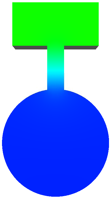
(a) $\kappa\approx 2.121-3.36\cdot 10^{-3}i$

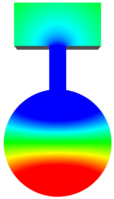
(b) $\kappa\approx 33.34-3.66\cdot 10^{-2}i$

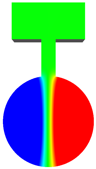
(c) $\kappa\approx 33.59-6.8510^{-11}i$

Figure 5: Real part of three resonance functions and corresponding resonances of a single Helmholtz resonator with volume $1\mathrm{l}$, length of the neck $5\mathrm{cm}$ and cross sectional area of the neck $3\mathrm{cm}^{2}$.

Fig. 5 gives cross-sections of a single Helmholtz resonator with three different resonance functions and the corresponding resonances. For $c=343m/s$ we calculate the frequency $f=c\Re(\kappa)/2\pi\approx 115.8Hz$, of the most relevant first resonance which has a quality factor $Q=\Re(\kappa)/|\Im(\kappa)|\approx 631$. The approximative formula (see e.g. [37]) for a Helmholtz resonator with volume $V$, neck length $L$ and cross sectional area of the neck $S$ gives $f=\frac{c}{2\pi}\sqrt{\frac{S}{LV}}\approx 133Hz$.

For these computations a mesh of $2477$ tetrahedrons with finite element order $7$, the number of degrees of freedom in radial direction $N=15$ and $\kappa_{0}=8$ lead to approximately $155000$ degrees of freedom. Note, that the third resonance in Fig. 5 has multiplicity $2$.

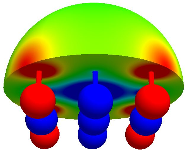
Figure 6: Real part of the total field to an incident plane wave $u_{i}(x)=e^{i\kappa d\cdot x}$ with $d=(-1/\sqrt{2},0,-1/\sqrt{2})^{T}$ and $\kappa=2.1241$. The values of the total field vary between $\pm 2000$, but the figure is limited to values between $\pm 10$.

Fig. 6 shows the real part of the total field to an incident plane wave with wavenumber $\kappa=2.1241$ for $9$ uniformly distributed resonators. For this system of resonators the first $9$ resonance frequencies are between $114.8Hz$ ($\kappa\approx 2.103$) and $116.1Hz$ ($\kappa\approx 2.126$) with quality factors between from $162$ to $864765$. For the resonance computations of the system of resonators we used a mesh with $24394$ tetrahedrons, finite element order $7$, $N=15$ and $\kappa_{0}=4$.

5.2 Convergence test of a magnetic dipole

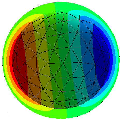
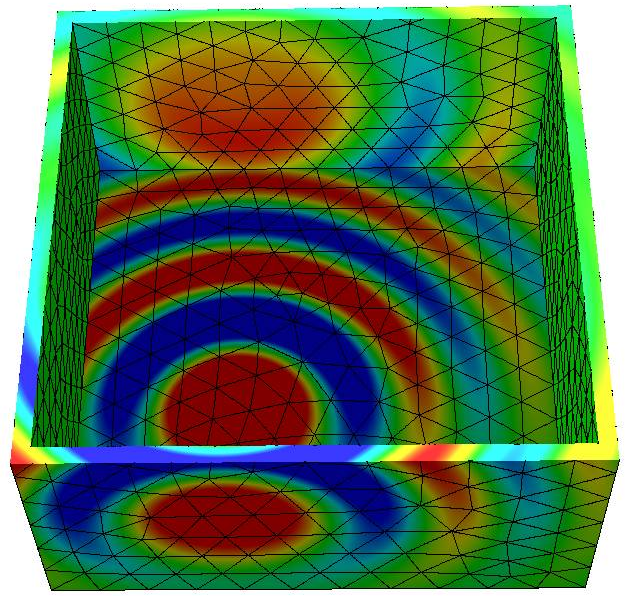
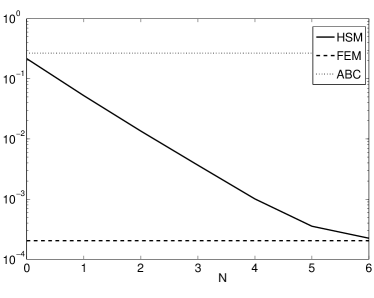
Figure 7: Right: $H(\operatorname{\rm\bf curl},\Omega_{\rm int})$-error of the HSM w.r.t. the number $N$ of degrees of freedom in radial direction compared to the finite element error and the error of a first order absorbing boundary condition for the two different domains $\Omega_{\rm int}$ on the left; Left: Cross-section of one Cartesian component of a magnetic dipole

In this example we resolve a magnetic dipole located at a point $y$

$$E_{y}(x)=\nabla_{x}\times\left(\frac{e^{i\kappa|x-y|}}{|x-y|}\left(\!\!\begin{array}[]{c}1\\ 1\\ 1\end{array}\!\!\right)\right)$$

in two different geometries (see Fig. 7). $E_{y}$ is a radiating solution of (1) with given wavenumber $\kappa>0$ and an unbounded domain $\Omega$, which does not contain the center $y$.

In the upper part of Fig. 7 the interior domain is the intersection of two balls with radius $5$ and $6$ ( $\Omega_{\rm int}=B_{6}\setminus B_{5}$), $\kappa=1$ and the center of the dipole is the origin ($y=0$). For the interior boundary $\partial B_{5}$ we use a Dirichlet boundary condition given by the tangential part of $E_{y}$. For the exterior boundary $\partial B_{6}$ we have three different cases: First we again use the exact Dirichlet boundary condition in order to compute the error of the finite element discretization of $\Omega_{\rm int}$ with polynomial order $6$. Second we use the first order absorbing boundary condition $\nabla\times E\times\nu-i\kappa E=0$ coming from the Silver-Müller radiation condition, which can be applied without spending additional degrees of freedom. Last we use the Hardy space method with $\kappa_{0}=10$, reference point $V_{0}=(0,0,0)$ and $N=0,\dots,8$ , which leads to $102279$ ($N=0$) up to $229975$ ($N=8$) degrees of freedom.

In the lower part of Fig. 7 the interior domain is the intersection of two cubes $\Omega_{\rm int}=[-3.2,3.2]^{3}\setminus[-3,3]^{3}$, $\kappa=5$ and the dipole is located at $y=(1,1.5,-1)^{T}$. The finite element method needs $555480$ degrees of freedom for polynomial order $5$; together with the Hardy space method with $\kappa_{0}=12.5$ and $V_{0}=(0,0,0)^{T}$ we get $584642$ up to $1080374$ degrees of freedom.

Both cases show a fast convergence of the Hardy space method, such that setting $N=4$ ($N=6$) suffices to reach the finite element error.

5.3 Cavity resonances

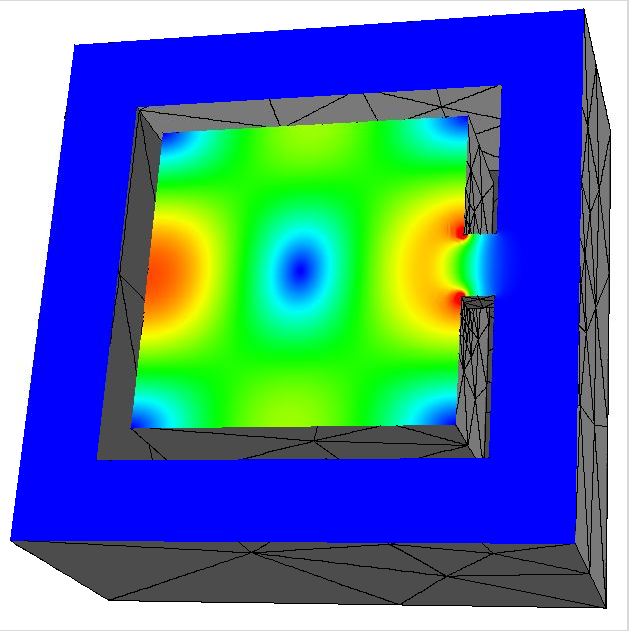
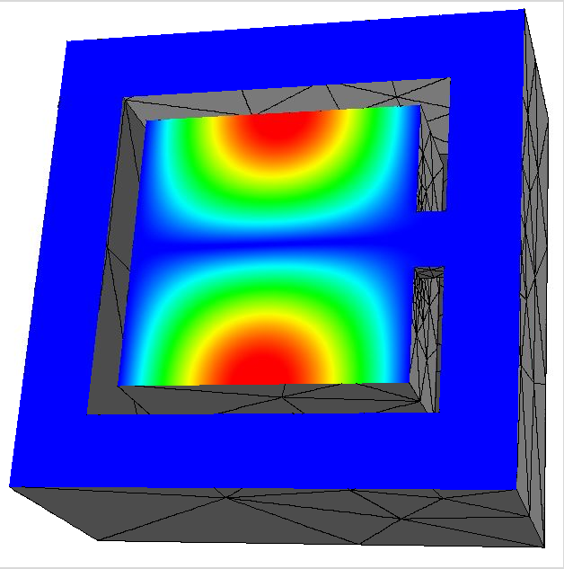
Figure 8: Cross-section of the absolute value of the two resonance functions of the resonances close to $\kappa=\sqrt{3}\frac{\pi}{2}\approx 2.72$

Here we search for resonances $\kappa\neq 0$ and radiating electric fields $E\neq 0$ solving (1) for $\Omega=\mathbb{R}^{3}\setminus K$ and $K=[-1.2,1.2]^{3}\setminus\left([-1,1]^{3}\cup[1,1.2]\times[-0.2,0.2]^{2}\right)$. Additionally, $E$ has to satisfy at $\partial K$ the perfectly conducting boundary conditions $E\times\nu=0$ with $\nu$ being the outward normal vector. This problem is an extension of the two dimensional acoustic open cavity problem in [19]. A similar acoustic problem is treated in [27] with boundary element methods.

In Fig. 8 the absolute value of two resonance functions on a cross-section of the interior domain $\Omega_{\rm int}=[-1.7,1.7]^{3}\cap\Omega$ is shown. For a closed cavity ($\Omega=[-1,1]^{3}$), the resonances are positive and analytically given by (see [1]) $\kappa=\sqrt{l+m+n}\frac{\pi}{2}$ for $l,m,n\in\mathbb{N}_{0}$ such that $lm+ln+mn>0$ The resonance functions in Fig. 8 belong to resonances close to the second cavity resonance $\kappa=\sqrt{3}\frac{\pi}{2}$ with multiplicity $2$.

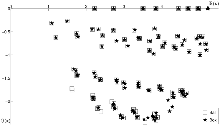
Figure 9: Resonances of an open cavity for two different discretizations: First $\Omega_{\rm int}=B_{2.5}\cap\Omega$, $\kappa_{0}=5$, $N=10$ and finite element order $5$. Second $\Omega_{\rm int}=[-1.7,1.7]^{3}\cap\Omega$, $\kappa_{0}=4-i$, $N=6$ and finite element order $6$

Fig. 9 shows the real and imaginary part of the computed resonances for two different discretizations. For the first we use the domain $\Omega_{\rm int}=B_{2.5}\cap\Omega$ with $\kappa_{0}=5$, $N=10$ and finite element order $5$ and in total $358924$ degrees of freedom. For the second dicretization $\Omega_{\rm int}=[-1.7,1.7]^{3}\cap\Omega$, $\kappa_{0}=4-i$, $N=6$ and finite element order $6$ lead to $390548$ degrees of freedom. Both discretizations give similar results for the cavity resonances near the real axis. The multiplicity of the resonances is not visible in Fig. 9. It is the same as expected from the resonances of the closed cavity given in [1]. The exterior resonances with in absolute values larger imaginary parts are mostly identical for the two discretizations, but for the resonances at the bottom of Fig. 9 the discretizations are too coarse.

5.4 Resonances of GaAs pyramidal micro-cavities

A second example of cavity resonances is taken from [22]. The cavity is a pyramid with height $0.14142$ and a quadratic base of length $0.28284$ which is turned up-side down and mounted on top of an infinite pyramid. Choosing the apex of the pyramids as reference point $V_{0}=(0,0,0)$, the infinite pyramid is bounded by the infinite rays in direction $(1,1,-1)^{T}$, $(-1,1,-1)^{T}$, $(-1,1,-1)^{T}$ and $(-1,-1,-1)^{T}$. The computational domain $\Omega_{\rm int}$ is a cuboid given by the vertices $(-0.2,-0.2,-0.1)$ and $(0.2,0.2,0.2)$. The pyramids are made of GaAs ($\varepsilon=12.25$). In contrast to the first example the exterior domain outside the plotted interior domain consist of two different materials, namely air ($\varepsilon=1$) and the infinite GaAs pyramid ($\varepsilon=12.25$).

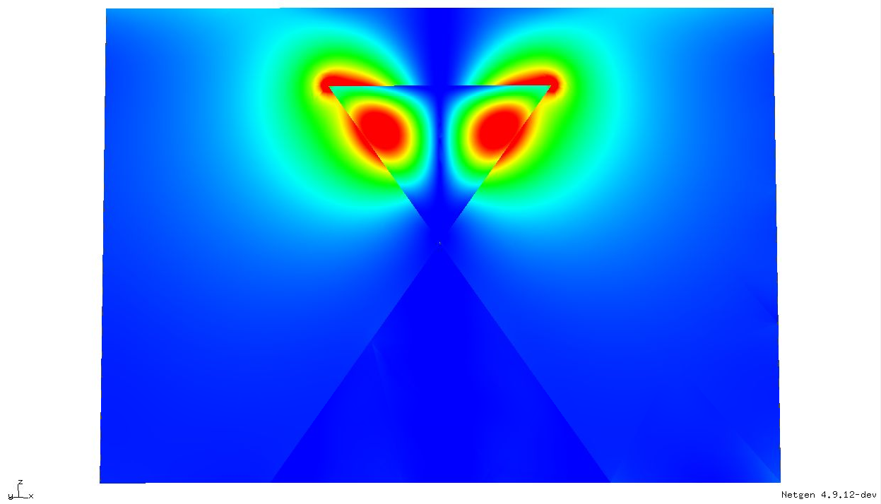
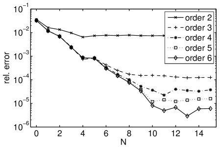
Figure 10: Left: Cross-section of the field intensity of the resonance function to the resonance $\kappa\approx 12.3034-0.8816i$. Right: Relative error of the computed resonance w.r.t. the number of degrees of freedom in radial direction for different finite element orders.

In Fig. 10 a cross-section of the field intensity of the resonance field for the resonance $\kappa\approx 12.3034-0.8816i$ is given.

To compute a reference solution $\Omega_{\rm int}$ is discretized by 2477 tetrahedrons and finite elements of order $7$ leading to approximately 1.5 million unknowns for the interior domain. For the exterior domain $18$ degrees of freedom in the radial direction cause in total 2 million unknowns. The error in Fig. 10 is the relative error of the computed resonance with respect to the reference resonance $\kappa\approx 12.3034-0.8816i$ for different finite element orders and different numbers of degrees of freedom in radial direction. The results indicate that depending on the finite element order only 8 to 10 degrees of freedom in radial direction are needed.

5.5 $(H(\operatorname{\rm div}),L^{2})$ resonance test

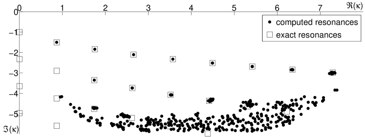
Figure 11: computed and exact acoustic resonances with $\Omega=\mathbb{R}^{3}\setminus B_{1}$, $\Omega_{\rm int}=[-1.2,1.2]^{3}\setminus B_{1}$, $\kappa_{0}=5-i$, reference point $V_{0}=0$ and $N=15$

In the last numerical test we compute acoustic resonances $\kappa$ outside a sphere with radius $1$. In this case the exact resonances are given by the roots of the spherical Hankel functions of the first kind, see [30, Example 3.24]. The multiplicity of a resonance is $2n+1$ if the resonance is the root of the $n$th Hankel function. Instead of solving the Helmholtz problem (2), we solve the mixed formulation (3) and use the $H(\operatorname{\rm div})$ and $L^{2}$ elements of Sections 3.3 and 3.4.

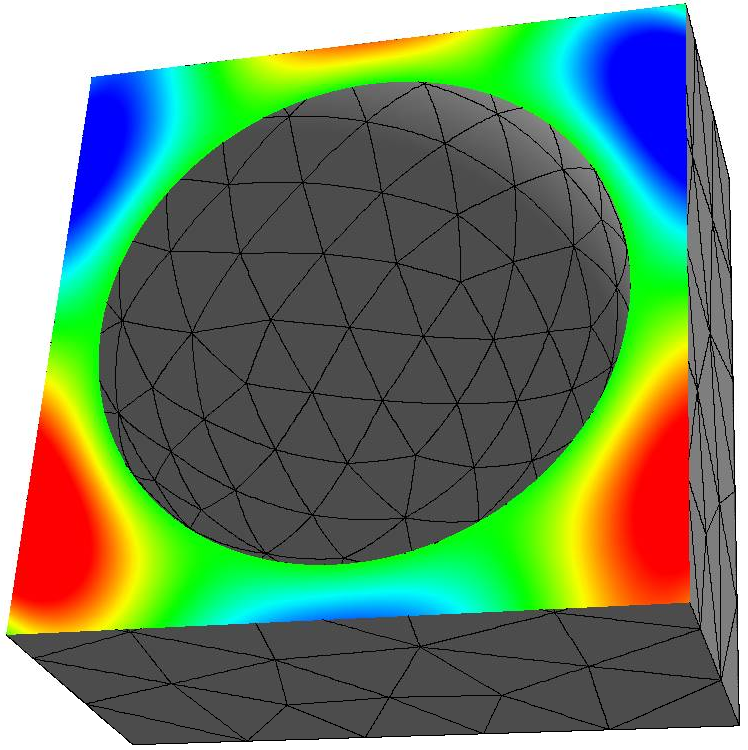
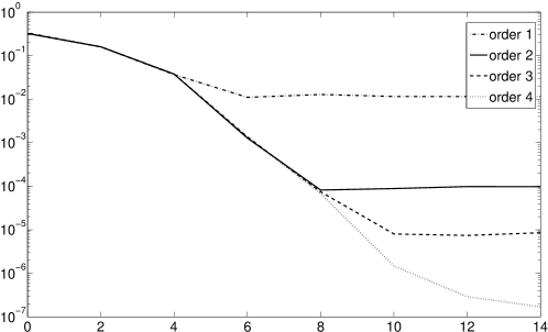
Figure 12: Left: Cross-section of one of the resonance functions to the resonance $\kappa\approx 1.754-1.839i$; right: relative error for different finite element orders and different $N$ of the computed resonance against the analytical one with $\Omega_{\rm int}=[-1.2,1.2]^{3}\setminus B_{1}$, $\kappa_{0}=7-0.3i$ and reference point $V_{0}=0$

In Fig. 11 the computed resonances $\kappa$ for $\Omega_{\rm int}=[-1.2,1.2]^{3}\setminus B_{1}$, finite element order $3$, $\kappa_{0}=5-i$, reference point $V_{0}=0$ and $N=15$ are compared to the analytical ones. Again, for the resonances with in absolute values larger imaginary part the discretization with in total $397316$ degrees of freedom is too coarse.

Fig. 12 shows the relative error of one computed resonance against one of the roots of the third spherical Hankel function of the first kind. In comparison to the results of Sec. 5.2 and Sec. 5.4 more degrees of freedom in radial direction are needed, since the Hardy space method has to resolve the Hankel function. In total $27256$ (order $1$, $N=0$) up to $549920$ (order $4$, $N=14$) degrees of freedom are used.

References

- [1] S. Adam, P. Arbenz, and R. Geus. Eigenvalue solvers for electromagnetic fields in cavities. Technical Report 275, Institute of Scientific Computing, ETH Zürich, 1997.
- [2] J.-P. Berenger. A perfectly matched layer for the absorption of electromagnetic waves. J. Comput. Phys., 114(2):185–200, 1994.
- [3] D. Boffi, P. Fernandes, L. Gastaldi, and I. Perugia. Computational models of electromagnetic resonators: analysis of edge element approximation. SIAM J. Numer. Anal., 36(4):1264–1290, 1999.
- [4] S. Burger, R. Köhle, L. Zschiedrich, W. Gao, F. Schmidt, R. März, and C. Nölscher. Benchmark of FEM, waveguide and FDTD algorithms for rigorous mask simulation. In M. P. Tracy Weed J., editor, SPIE - BACUS, advancement of photomask technology, volume 5992, 2005.
- [5] W. C. Chew and W. H. Weedon. A 3d perfectly matched medium from modified maxwell’s equations with stretched coordinates. Microwave Optical Tech. Letters, 7:590–604, 1994.
- [6] F. Collino and P. Monk. The perfectly matched layer in curvilinear coordinates. SIAM J. Sci. Comput., 19(6):2061–2090 (electronic), 1998.
- [7] D. Colton and R. Kress. Inverse acoustic and electromagnetic scattering theory, volume 93 of Applied Mathematical Sciences. Springer-Verlag, Berlin, second edition, 1998.
- [8] L. Demkowicz and F. Ihlenburg. Analysis of a coupled finite-infinite element method for exterior Helmholtz problems. Numer. Math., 88(1):43–73, 2001.
- [9] L. Demkowicz, J. Kurtz, D. Pardo, M. Paszyński, W. Rachowicz, and A. Zdunek. Computing with -adaptive finite elements. Vol. 2. Chapman & Hall/CRC Applied Mathematics and Nonlinear Science Series. Chapman & Hall/CRC, Boca Raton, FL, 2008. Frontiers: Three dimensional elliptic and Maxwell problems with applications.
- [10] L. Demkowicz and M. Pal. An infinite element for Maxwell’s equations. Comput. Methods Appl. Mech. Engrg., 164(1-2):77–94, 1998.
- [11] P. L. Duren. Theory of spaces. Pure and Applied Mathematics, Vol. 38. Academic Press, New York, 1970.
- [12] J. K. Gansel, M. Wegener, S. Burger, and S. Linden. Gold helix photonic metamaterials: A numerical parameter study. Opt. Express, 18(2):1059–1069, 2010.
- [13] D. Givoli. High-order local non-reflecting boundary conditions: a review. Wave Motion, 39:319–326, 2004.
- [14] M. J. Grote and J. B. Keller. Nonreflecting boundary conditions for Maxwell’s equation. J. Comput. Phys., 139:327–342, 1998.
- [15] T. Hagstrom. New results on absorbing layers and radiation boundary conditions. In Ainsworth, Mark (ed.) et al., Topics in computational wave propagation. Direct and inverse problems. Berlin: Springer. Lect. Notes Comput. Sci. Eng. 31, 1-42 . 2003.
- [16] S. Hein, T. Hohage, W. Koch, and J. Schöberl. Acoustic resonances in high lift configuration. J. Fluid Mech., 582:179–202, 2007.
- [17] P. J. Hilton and S. Wylie. Homology theory: An introduction to algebraic topology. Cambridge University Press, New York, 1960.
- [18] R. Hiptmair. Finite elements in computational electromagnetism. Acta Numer., 11:237–339, 2002.
- [19] T. Hohage and L. Nannen. Hardy space infinite elements for scattering and resonance problems. SIAM J. Numer. Anal., 47(2):972–996, 2009.
- [20] T. Hohage, F. Schmidt, and L. Zschiedrich. Solving time-harmonic scattering problems based on the pole condition. I. Theory. SIAM J. Math. Anal., 35(1):183–210, 2003.
- [21] G. C. Hsiao and W. L. Wendland. Boundary integral equations, volume 164 of Applied Mathematical Sciences. Springer-Verlag, Berlin, 2008.
- [22] M. Karl, D. Rülke, T. Beck, D. Hu, D. Schaadt, H. Kalt, and M. Hetterich. Reversed pyramids as novel optical micro-cavities. Superlattices and Microstructures, 47(1):83 – 86, 2010.
- [23] B. Kettner. Ein Algorithmus zur prismatoidalen Diskretisierung von unbeschränkten Außenräumen in 2D und 3D. Master’s thesis, Freie Universität Berlin, 2007.
- [24] B. Kettner and F. Schmidt. Meshing of heterogeneous unbounded domains. In Proceedings IMR17, 2008.
- [25] S. Kim and J. E. Pasciak. The computation of resonances in open systems using a perfectly matched layer. Math. Comp., 2008.
- [26] M. Lenoir, M. Vullierme-Ledard, and C. Hazard. Variational formulations for the determination of resonant states in scattering problems. SIAM J. Math. Anal., 23:579–608, 1992.
- [27] S. Marburg. Normal modes in external acoustics. part iii: Sound power evaluation based on superposition of frequency-independent modes. Acta Acustica united with Acustica, 92:296–311(16), 2006.
- [28] P. Monk. Finite element methods for Maxwell’s equations. Numerical Mathematics and Scientific Computation. Oxford University Press, New York, 2003.
- [29] G. J. Murphy. -algebras and operator theory. Academic Press Inc., Boston, MA, 1990.
- [30] L. Nannen. Hardy-Raum Methoden zur numerischen Lösung von Streu- und Resonanzproblemen auf unbeschränkten Gebieten. PhD thesis, University of Göttingen, Der Andere Verlag, Tönning, 2008.
- [31] L. Nannen and A. Schädle. Hardy space infinite elements for helmholtz-type problems with unbounded inhomogeneities. Wave Motion, In Press, 2010.
- [32] D. Ruprecht, A. Schädle, F. Schmidt, and L. Zschiedrich. Transparent boundary conditions for time-dependent problems. SIAM J. Sci. Comput., 30(5):2358–2385, 2008.
- [33] O. Schenk and K. Gärtner. Solving unsymmetric sparse systems of linear equations with PARDISO. In Computational science—ICCS 2002, Part II (Amsterdam), volume 2330 of Lecture Notes in Comput. Sci., pages 355–363. Springer, Berlin, 2002.
- [34] F. Schmidt. A new approach to coupled interior-exterior Helmholtz-type problems: Theory and algorithms. Habilitation, Freie Universität Berlin, 2002.
- [35] J. Schöberl. Netgen - an advancing front 2d/3d-mesh generator based on abstract rules. Comput.Visual.Sci, 1:41–52, 1997.
- [36] J. Schöberl and S. Zaglmayr. High order Nédélec elements with local complete sequence properties. COMPEL, 24(2):374–384, 2005.
- [37] M. Schroeder, T. D. Rossing, F. Dunn, W. M. Hartmann, D. M. Campbell, and N. H. Fletcher. Springer Handbook of Acoustics. Springer Publishing Company, Incorporated, 2007.
- [38] B. Simon. The definition of molecular resonance curves by the method of exterior complex scaling. Phys. Lett. A, 71A(2, 3), 1979.
- [39] S. Zaglemayr. High Order Finite Element Methods for Electromagnetic Field Computation. PhD thesis, Universität Linz, 2006.
- [40] L. Zschiedrich, R. Klose, A. Schädle, and F. Schmidt. A new finite element realization of the perfectly matched layer method for Helmholtz scattering problems on polygonal domains in two dimensions. J. Comput. Appl. Math., 188(1):12–32, 2006.