Software for Generation of Classes of Test Functions with Known Local and Global Minima for Global Optimization

Abstract

A procedure for generating non-differentiable, continuously differentiable, and twice continuously differentiable classes of test functions for multiextremal multidimensional box-constrained global optimization and a corresponding package of C subroutines are presented. Each test class consists of 100 functions. Test functions are generated by defining a convex quadratic function systematically distorted by polynomials in order to introduce local minima. To determine a class, the user defines the following parameters: (i) problem dimension, (ii) number of local minima, (iii) value of the global minimum, (iv) radius of the attraction region of the global minimizer, (v) distance from the global minimizer to the vertex of the quadratic function. Then, all other necessary parameters are generated randomly for all 100 functions of the class. Full information about each test function including locations and values of all local minima is supplied to the user. Partial derivatives are also generated where possible.

Key Words: Global optimization, test problems generation, known local minima

1 Introduction

A wide literature is dedicated to development of numerical algorithms for solving the global optimization problem (see, for example, references given in [7]). The problem may be formulated as

$$f^{*}=f(x^{*})=\min_{x\in\mathcal{F}}f(x),\ \ \mathcal{F}\subset\mathbb{R}^{N},$$ (1)

where $f(x)$ is a multiextremal and possibly non-differentiable function and $\mathcal{F}$ is a compact set.

One of the approaches to studying and verifying validity of numerical algorithms is their comparison on test problems (see, e.g., [1], [2], [3], [4], [5], [6], [7], [8], [9], [12], [13], [14], [15], [16], [17]; [18], [19], [20]; [21], [22], [23]). Many global optimization tests were taken from real-life problems and for this reason comprehensive information about them is not available. The number of local minima may be unknown, as well as their locations, regions of attraction, and even values (including that of the global minimum).

Recently [6] introduced two types of functions with a priori known local minima and their regions of attraction. The tests proposed take a convex quadratic function (called hereafter ‘paraboloid’) systematically distorted by cubic polynomials and by quintic polynomials to introduce local minima and to construct test functions that are continuously differentiable in some region $\Omega\supseteq\mathcal{F}$ (called hereafter ‘D-type’ test functions) and twice continuously differentiable in $\Omega\supseteq\mathcal{F}$ (called hereafter ‘D2-type’ test functions), where $\mathcal{F}$ is from (1) and $\Omega$ is a hyperrectangle.

To define a function of one of these types it is necessary to determine a number of correlated parameters. Unfortunately, the correlations do not allow simple and fast generation of the test functions. Additionally, generation of different functions having similar properties becomes difficult and non-intuitive when dimension and/or number of local minima increase.

In this paper, in addition to the two types of test functions from [6], the third type of non-differentiable test functions (called hereafter ‘ND-type’) is presented and a generator for these three types of test functions is proposed. The software to be introduced generates classes of test functions and provides procedures for calculating the first order derivatives of the D-type test functions and the first and second order derivatives of the D2-type test functions.

Each class contains 100 functions and is defined by the following parameters (the only ones to be determined by the user):

1. problem dimension;

2. number of local minima;

3. value of the global minimum;

4. radius of the attraction region of the global minimizer;

5. distance from the global minimizer to the vertex of the paraboloid.

The other necessary parameters (i.e., locations of all minimizers, their regions of attraction, and values of minima) are chosen randomly by the generator. After generation a special notebook containing a complete description of all the functions from the generated class is supplied to the user.

The rest of the paper is structured as follows. In Section 2, a mathematical description of the three types of test functions is given. Section 3 introduces the generator and details of its implementation. Section 4 is devoted to usage of the generator.

2 Mathematical description

In this section, the three types of test functions are briefly described. Let us start with the D-type and D2-type functions (see [6]). A function $f(x)$ of the D-type is determined over an admissible region $\Omega\supseteq\mathcal{F}$, where $\mathcal{F}$ is from (1) and

$$\Omega=[a,b\,]=\{x\in\mathbb{R}^{N}\,:\,a\leq x\leq b\},\hskip 8.53581pta<b,\hskip 5.69054pta,b\in\mathbb{R}^{N}.$$ (2)

The function is constructed by modifying a paraboloid $Z$:

$$Z:\ g(x)=\|x-T\|^{2}+\,t,\ \ x\in\Omega,$$ (3)

(hereafter $\|\cdot\|$ denotes the Euclidean norm) with the minimum $t$ at a point $T\in{\rm int}(\Omega)$ in such a way that the resulting function $f(x)$ has $m$, $m\geq 2$, local minimizers: point $T$ from (3) (we denote it by $M_{1}:=T$) and points

$$M_{i}\in{\rm int}(\Omega),\ \ M_{i}\neq T,\ M_{i}\neq M_{j},\ \ i,j=2,\ldots,m,\ i\neq j.$$ (4)

The paraboloid $Z$ from (3) is modified by a function $C_{i}(x)$, which is constructed by using cubic polynomials within balls $S_{i}\subset\Omega$ around each point $M_{i}$, $i=2,\ldots,m$, where

$$S_{i}=\{x\in\mathbb{R}^{N}:\,\|x-M_{i}\|\ \leq\rho_{i},\,\rho_{i}>0\},\ \ i=1,\ldots,m.$$ (5)

Functions $Q_{i}(x)$, $i=2,\ldots,m$, use quintic polynomials to determine the D2-type test functions.

Selection of radii $\rho_{i}$, $i=1,\ldots,m$, is carried out in such a manner that sets $S_{i}$ from (5) do not overlap:

$$S_{i}\cap S_{j}=\varnothing,\ \ i,j=1,\ldots,m,\ i\neq j.$$ (6)

It is not required that each attraction region $S_{i}$, $i=1,\ldots,m$, be entirely contained in $\Omega$. Note that we use the notation “attraction region” with respect to the balls $S_{i}$, $i=1,\ldots,m$, just for simplicity. Naturally, definition of the real attraction region for each local minimizer will depend on the method used for optimization and will change from one algorithm to another.

Formally, D-type functions [6] are described as follows:

$$f(x)=\left\{\begin{array}[]{ll}C_{i}(x),&x\in S_{i},\,i\in\{2,\ldots,m\},\\ g(x),&x\notin S_{2}\cup\ldots\cup S_{m}\,,\end{array}\right.$$ (7)

where $g(x)$ is from (3), sets $S_{i}$, $i=2,\ldots,m$, from (5) satisfy (6), and

$$C_{i}(x)=\left(\frac{2}{\rho_{i}^{2}}\frac{<\!x-M_{i},\,T-M_{i}\!>}{\|x-M_{i}\|}-\frac{2}{\rho_{i}^{3}}A_{i}\right)\|x-M_{i}\|^{3}+$$

$$+\left(1-\frac{4}{\rho_{i}}\frac{<\!x-M_{i},\,T-M_{i}\!>}{\|x-M_{i}\|}+\frac{3}{\rho_{i}^{2}}A_{i}\right)\|x-M_{i}\|^{2}+f_{i}.$$ (8)

In (8) radii $\rho_{i}$, $i=2,\ldots,m$, determine the sets $S_{i}$ from (5), $<\!\cdot,\cdot\!>$ denotes the usual scalar product, and the values $A_{i}$, $i=2,\ldots,m$, are found as

$$A_{i}=\|T-M_{i}\|^{2}+t-f_{i},$$ (9)

where $f_{1}=t$ and $f_{i}$, $i=2,\ldots,m$, are the function values at local minimizers $M_{i}$:

$$f_{i}=\min\{g(x)\,:x\in B_{i}\}-\gamma_{i},\ \ \gamma_{i}>0,$$ (10)

where $B_{i}$ is the boundary of the ball $S_{i}$:

$$B_{i}=\{x\in\mathbb{R}^{N}:\,\|x-M_{i}\|\ =\rho_{i},\,\rho_{i}>0\},\ \ i=2,\ldots,m,$$ (11)

and $\gamma_{i}$ is a parameter ensuring that the value $f_{i}$ is less than the minimum of the paraboloid $Z$ from (3) over $B_{i}$.

Analogously, D2-type functions [6] are defined by

$$f(x)=\left\{\begin{array}[]{ll}Q_{i}(x),&x\in S_{i},\,i\in\{2,\ldots,m\},\\ g(x),&x\notin S_{2}\cup\ldots\cup S_{m}\,,\end{array}\right.$$ (12)

where

$$Q_{i}(x)=\left[-\frac{6}{\rho_{i}^{4}}\frac{<\!x-M_{i},\,T-M_{i}\!>}{\|x-M_{i}\|}+\frac{6}{\rho_{i}^{5}}A_{i}+\frac{1}{\rho_{i}^{3}}(1-\frac{\delta}{2})\right]\|x-M_{i}\|^{5}+$$

$$\left[\frac{16}{\rho_{i}^{3}}\frac{<\!x-M_{i},\,T-M_{i}\!>}{\|x-M_{i}\|}-\frac{15}{\rho_{i}^{4}}A_{i}-\frac{3}{\rho_{i}^{2}}(1-\frac{\delta}{2})\right]\|x-M_{i}\|^{4}+$$

$$\left[-\frac{12}{\rho_{i}^{2}}\frac{<\!x-M_{i},\,T-M_{i}\!>}{\|x-M_{i}\|}+\frac{10}{\rho_{i}^{3}}A_{i}+\frac{3}{\rho_{i}}(1-\frac{\delta}{2})\right]\|x-M_{i}\|^{3}+$$

$$\frac{1}{2}\delta\|x-M_{i}\|^{2}+f_{i}$$ (13)

with $A_{i}$ and $f_{i}$, $i=2,\ldots,m$, from (9) and (10), and $\delta$ is an arbitrary positive real number (see [6, Lemma 3.1]).

The properties of these functions have been studied by [6]. In particular, the following results can be proved:

i. D-type functions (7)–(8) are continuously differentiable in $\Omega$ [6, Lemma 2.1].

ii. D2-type functions (12)–(13) are twice continuously differentiable in $\Omega$ [6, Lemma 3.1].

Let us now describe the ND-type test functions, which are continuous in $\Omega$ but non-differentiable in the whole region $\Omega$. An analogous procedure is considered: the paraboloid $Z$ from (3) is modified by a function $P_{i}(x)$ constructed from second degree polynomials within each region $S_{i}\subset\Omega$ from (5) in such a way that the resulting function $f(x)$ is continuous in the feasible region $\Omega$ from (2), differentiable at each local minimizer $M_{i}$, $i=2,\ldots,m$, from (4), but generally non-differentiable at the points of the boundaries $B_{i}$ of the balls $S_{i}$, $i=2,\ldots,m$, determined by (11). That is,

$$f(x)=\left\{\begin{array}[]{ll}P_{i}(x),&x\in S_{i},\,i\in\{2,\ldots,m\},\\ g(x),&x\notin S_{2}\cup\ldots\cup S_{m}\,,\end{array}\right.$$ (14)

where $g(x)$ is from (3), sets $S_{i}$, $i=2,\ldots,m$, from (5) satisfy (6), and

$$P_{i}(x)=\left(1-\frac{2}{\rho_{i}}\frac{<\!x-M_{i},\,T-M_{i}\!>}{\|x-M_{i}\|}+\frac{1}{\rho_{i}^{2}}A_{i}\right)\|x-M_{i}\|^{2}+f_{i}.$$ (15)

In (15) the values $\rho_{i}$, $A_{i}$, and $f_{i}$ ($i=2,\ldots,m$) are determined in the same way as for the D- and D2-type functions by formulae (5)–(6), (9), and (10), respectively.

3 Generation of tests classes

As one can see from the previous section, all three function types have many parameters to be coordinated. Moreover, their characteristics (for example, the mutual positions of the local minimizers, the global minimizer, and the paraboloid vertex; the size of the attraction regions of local minimizers; the function values at local minima) influence the properties of the test functions significantly from the point of view of global optimization algorithms. For example, coincidence of the global minimizer with the paraboloid vertex leads to generation of too simple functions. Existence of many deep minima having narrow regions of attraction can lead to the impossibility of global minimizer location even by the most “intelligent” global optimization algorithms. All these features should be added to the general scheme from Section 2 in order to obtain well-structured test classes.

In the generator, the user sets just a few parameters defining a desirable class while all the other parameters are chosen randomly. The generator is also employed in maintaining conditions distinguishing each class – for example, the distance of the global minimizer from the minimizer of the paraboloid, dependence of the local minima values on the attraction regions sizes, etc. Thus, the generator gives the researcher the ability to construct classes of 100 test functions of arbitrary dimension with arbitrary number of local minima.

This section describes how a class consisting of D-type test functions is generated. Classes consisting of D2-type and ND-type functions are constructed analogously.

Each test class generated by the introduced software contains 100 test functions $f(x)$ and is defined by the following parameters to be fixed by the user:

1. the problem dimension $N$, $N\geq 2$;

2. the number of local minimizers $m$, $m\geq 2$, including the minimizer $T$ for the paraboloid (3) (all the minimizers are chosen randomly);

3. the global minimum value $f^{*}$, the same for all the functions of the class;

4. the radius $\rho^{*}$ of the attraction region of the global minimizer $x^{*}$;

5. the distance $r^{*}$ from the paraboloid vertex $T$ to the global minimizer $x^{*}\in\Omega$ (whose coordinates are also chosen randomly).

By changing these parameters the user can create classes with different properties.

Each function of a test class is specified by its number $n$, $1\leq n\leq 100$. The other parameters of the functions from (3)–(15) are chosen randomly by means of the random number generator proposed in [10].

The input parameters $f^{*}$, $r^{*}$, and $\rho^{*}$ must be chosen in such a way that the following simple conditions are satisfied:

$$f^{*}<t$$ (16)

(which means that the global minimizer is not a vertex of the paraboloid; this requirement allows us to avoid too simple functions with a global minimum at the vertex of the paraboloid $Z$ from (3)),

$$0<r^{*}<0.5\min_{1\leq j\leq N}|b(j)-a(j)|$$ (17)

(i.e., the global minimizer $x^{*}$ belongs to the admissible region $\Omega$ even in the case when the paraboloid vertex $T$ is at the center of $\Omega$), and

$$0<\rho^{*}\leq 0.5r^{*}.$$ (18)

Note that it is not required that each attraction region $S_{i}$, $i=1,\ldots,m$, from (5) entirely belongs to $\Omega$.

The admissible region $\Omega$ is taken as $\Omega=[-1,1]^{N}$ and the minimal value of the paraboloid (3) is fixed at $t=0$ by default (naturally, these parameters can be changed by the user).

Let us discuss in more detail the random procedure generating parameters for test functions. (The unique difference for the D2-type is that the parameter $\delta$ from (13) is required; this parameter is chosen randomly from the open interval $(0,\Delta)$, where $\Delta$ is a positive number taken by default $\Delta=10$.) Hereafter the vertex $T$ from (3) in the set (4) of local minimizers has the index 1, $M_{1}:=T$, and the global minimizer $x^{*}$ has the index 2, $M_{2}:=x^{*}$. Naturally, among the minimizers $M_{i}$, $i=3,\ldots,m$, another global minimizer $y^{*}\neq x^{*}$ can be generated.

First, coordinates of the paraboloid vertex $T$, coordinates of the global minimizer $x^{*}$, and coordinates of the remaining local minimizers $M_{i}$ (controlling the satisfaction of (4)) are chosen randomly. Then, the attraction regions radii $\rho_{i}$, $i\neq 2$, from (5) are determined: to do this the attraction regions of each local minimizer from (4) ($i\neq 2$ because the attraction region of the global minimizer is fixed: $\rho_{2}=\rho^{*}$) are expanded until condition (6) is not violated. Finally, values of the function $f(x)$ at local minima $M_{i}$, $i=3,\ldots,m$, are fixed by choosing random values $\gamma_{i}$, $i=3,\ldots,m$, from (10) (recall that $f_{1}=t$ and $f_{2}=f^{*}$).

Let us consider these three principal operations in detail.

Coordinates of the local minimizers $M_{i}$, $i=3,\ldots,m$, from (4), coordinates of the vertex $T$ of the paraboloid (3), and location of the global minimizer $x^{*}$ are chosen randomly at the intersection of $\Omega$ and the sphere of radius $r^{*}$ with a center at $T$ so that (4) is satisfied. For the positioning of $x^{*}$ we use generalized spherical coordinates

$$x^{*}_{j}:=T_{j}+r^{*}\cos\phi_{j}\prod_{k=1}^{j-1}\sin\phi_{k},\ \ j=1,\ldots,N-1,$$

$$x^{*}_{N}:=T_{N}+r^{*}\prod_{k=1}^{N-1}\sin\phi_{k},$$ (19)

where the components of the vector

$$\phi=(\phi_{1},\ldots,\phi_{N})\in\Phi=\{0\leq\phi_{1}\leq\pi;\ 0\leq\phi_{j}\leq 2\pi,\ j=2,\ldots,N\}$$

are chosen randomly. In this case, if some $x^{*}_{k}\notin\Omega$, $1\leq k\leq N$, this coordinate is redefined as

$$x^{*}_{k}:=2T_{k}-x^{*}_{k}.$$

After selection of coordinates of the paraboloid vertex $T$ and of the global minimizer $x^{*}$, coordinates of the points $M_{i}$, $i=3,\ldots,m$, are generated in such a way that beside condition (4) the condition

$$\|M_{i}-x^{*}\|-\rho^{*}=\zeta,\ \ \zeta>0$$ (20)

is satisfied with some positive parameter $\zeta$. This condition follows from (6) and does not allow the local minimizers to be very close to the attraction region of the global minimizer $x^{*}$. Thus, in (20) the parameter $\zeta$ should not be too small. The value $\zeta=\rho^{*}$ is chosen by default.

The next step of the test function construction sets attraction regions. Each value $\rho_{i}$, $i\neq 2$, from (5) is initially calculated as half of the minimum distance between the minimizer $M_{i}$ and the remaining local minimizers

$$\rho_{i}:=0.5\min_{1\leq j\leq m,\ j\neq i}\|M_{i}-M_{j}\|,\ \ i=1,\ldots,m,\ i\neq 2,$$

$$\rho_{2}:=\rho^{*}$$ (21)

(in such a way that the attraction regions from (5) do not overlap). Then, an attempt to increase the values $\rho_{i}$, $i=1,\ldots,m$, $i\neq 2$ (i.e., an attempt to enlarge the attraction regions) is made:

$$\rho_{i}:=\max\left(\rho_{i},\min_{1\leq j\leq m,\ j\neq i}\{\|M_{i}-M_{j}\|-\rho_{j}\}\right),\ \ i=1,\ldots,m,\ i\neq 2.$$ (22)

Because of the recursive character of formulae (22), an expansion of the attraction regions depends on the order in which these regions are selected (an ascending order of the indices is chosen).

Finally, the values of the radii $\rho_{i}$ are corrected by the weight coefficients $w_{i}$:

$$\rho_{i}:=w_{i}\,\rho_{i},\ \ i=1,\ldots,m,$$

where $0<w_{i}\leq 1$, $i=1,\ldots,m$, and the values $w_{i}$ are chosen by default as

$$w_{i}=0.99,\ \ i=1,\ldots,m,\ i\neq 2,\hskip 19.91692pt{\rm and}\hskip 19.91692ptw_{2}=1.$$ (23)

At the last step the function values $f_{i}$, $i=3,\ldots,m$, at the local minima are generated by using formula (10), where $\gamma_{i}$ must be specified. Each value $\gamma_{i}$, $i=3,\ldots,m$, is chosen (note that the values $\gamma_{1}$ and $\gamma_{2}$ are not considered because the function values $f_{1}=t$ at the paraboloid vertex and $f_{2}=f^{*}$ at the global minimizer have been fixed by the user without using (10)) as the minimum of two values generated randomly from the open intervals $(\rho_{i},2\rho_{i})$ and $(0,Z_{B_{i}}-f^{*})$, where $Z_{B_{i}}$ is the minimum of the paraboloid $Z$ from (3) over $B_{i}$ from (11). In such a way, the values $f_{i}$ in (10) depend on radii $\rho_{i}$ of the attraction regions $S_{i}$, $i=3,\ldots,m$, and at the same time the following condition is satisfied:

$$f^{*}\leq f_{i},\ \ i=3,\ldots,m.$$

Note that dependence of the function values at local minima on the radii of the attraction regions is not respected by the global optimum value $f_{2}=f^{*}$ because the user defines the function value at the global minimizer and the radius $\rho^{*}$ of its region of attraction directly when choosing the corresponding test class.

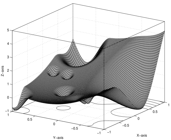
Figure 1: The function number 9 from a class of two-dimensional D-type test functions with 10 local minima

Figure 1 shows an example of the D-type test function. This function is defined in the region $\Omega=[-1,1]^{2}$ and is number 9 in the class of D-type functions with the following parameters:

1. dimension $N=2$;

2. number of local minima $m=10$;

3. value of the global minimum $f^{*}=-1$;

4. radius of the attraction region of the global minimizer $\rho^{*}=\frac{1}{3}$;

5. distance from the global minimizer $x^{*}$ to the vertex $T$ of the paraboloid from (3) is $r^{*}=\frac{2}{3}$.

The generated global minimizer of this function is $x^{*}=(-0.911,0.989)$ and the paraboloid minimizer is $T=(-0.711,0.353)$.

4 Usage of the test classes generator

The generator package has been written in ANSI Standard C and successfully tested on Windows and UNIX platforms. Our implementation follows the procedure described in Section 3. First, the general structure of the package is described, then instructions for using the test classes generator (called hereafter GKLS-generator) are given.

4.1 Structure of the package

The package includes the following files:

gkls.c

– the main file;

gkls.h

– the header file that users should include in their application projects in order to call subroutines from the file gkls.c;

rnd_gen.c

– the file containing the uniform random number generator proposed in Knuth [[10]; [11]];

rnd_gen.h

– the header file for linkage to the file rnd_gen.c;

example.c

– an example of the GKLS-generator usage;

Makefile

– an example of a UNIX makefile provided to UNIX users for a simple compilation and linkage of separate files of the application project.

For implementation details the user can consult the C codes. Note that the random number generator in rnd_gen.c uses the logical-and operation ‘&’ for efficiency, so it is not strictly portable unless the computer uses two’s complement representation for integer. It does not limit portability of the package because almost all modern computers are based on two’s complement arithmetic.

4.2 Calling sequence for generation and usage of the tests classes

Here we describe how to generate and use classes of the ND-, D-, and D2-type test functions. Again, we concentrate on the D-type functions. The operations for the remaining two types are analogous.

To utilize the GKLS-generator the user must perform the following steps:

Step 1.

Input of the parameters defining a specific test class.

Step 2.

Generating a specific test function of the defined test class.

Step 3.

Evaluation of the generated test function and, if necessary, its partial derivatives.

Step 4.

Memory deallocating.

Let us consider these steps in turn.

4.2.1 Input of the parameters defining a specific test class

This step is subdivided into: (a) defining the parameters of the test class, (b) defining the admissible region $\Omega$, and (c) checking (if necessary).

– (a) Defining the parameters of the test class. The parameters to be defined by the user determine a specific class (of the ND-, D- or D2-type) of 100 test functions (a specific function is retrieved by its number). There are the following parameters:

GKLS_dim

– (unsigned int) dimension $N$ (from (1)) of test functions; $N\geq 2$ (since multidimensional problems are considered in (1)) and $N<$ NUM_RND in rnd_gen.h; this value is limited by the power of unsigned int-representation; default $N=2$;

GKLS_num_minima

– (unsigned int) number $m$ (from (4)) of local minima including the paraboloid $Z$ minimum (from (3)) and the global minimum; $m\geq 2$; the upper bound of this parameter is limited by the power of unsigned int-representation; default $m=10$;

GKLS_global_value

– (double) global minimum value $f^{*}$ of $f(x)$; condition (16) must be satisfied; the default value is $-1.0$ (defined in the file gkls.h as a constant GKLS_GLOBAL_MIN_VALUE);

GKLS_global_dist

– (double) distance $r^{*}$ from the paraboloid vertex $T$ in (3) to the global minimizer $x^{*}\in\Omega$ of $f(x)$; condition (17) must be satisfied; the default value is

$${\rm GKLS\_global\_dist}\ \stackrel{{\scriptstyle\rm def}}{{=}}\ \min_{1\leq j\leq N}|b(j)-a(j)|/\,3,$$

where the vectors $a$ and $b$ determine the admissible region $\Omega$ in (2);

GKLS_global_radius

– (double) radius $\rho^{*}$ of the attraction region of the global minimizer $x^{*}\in\Omega$ of $f(x)$; condition (18) must be satisfied; the default value is

$${\rm GKLS\_global\_radius}\ \stackrel{{\scriptstyle\rm def}}{{=}}\ \min_{1\leq j\leq N}|b(j)-a(j)|/\,6.$$

The user may call subroutine GKLS_set_default() to set the default values of these five variables.

– (b) Defining the admissible region $\Omega$. With $N$ determined, the user must allocate dynamic arrays GKLS_domain_left and GKLS_domain_right to define the boundary of the hyperrectangle $\Omega$. This is done by calling subroutine

int GKLS_domain_alloc ();
which has no parameters and returns the following error codes defined in gkls.h:

GKLS_OK

– no errors;

GKLS_DIM_ERROR

– the problem dimension is out of range; it must be greater than or equal to 2 and less than NUM_RND defined in rnd_gen.h;

GKLS_MEMORY_ERROR

– there is not enough memory to allocate.

The same subroutine defines the admissible region $\Omega$. The default value $\Omega=[-1,1]^{N}$ is set by GKLS_set_default().

– (c) Checking. The following subroutine allows the user to check validity of the input parameters:

int GKLS_parameters_check ().
It has no parameters and returns the following error codes (see gkls.h):

GKLS_OK

– no errors;

GKLS_DIM_ERROR

– problem dimension error;

GKLS_NUM_MINIMA_ERROR

– number of local minima error;

GKLS_BOUNDARY_ERROR

– the admissible region boundary vectors are ill-defined;

GKLS_GLOBAL_MIN_VALUE_ERROR

– the global minimum value is not less than the paraboloid (3) minimum value $t$ defined in gkls.h as a constant GKLS_PARABOLOID_MIN;

GKLS_GLOBAL_DIST_ERROR

– the parameter $r^{*}$ does not satisfy (17);

GKLS_GLOBAL_RADIUS_ERROR

– the parameter $\rho^{*}$ does not satisfy (18).

4.2.2 Generating a specific test function of the defined test class

After a specific test class has been chosen (i.e., the input parameters have been determined) the user can generate a specific function that belongs to the chosen class of 100 test functions. This is done by calling subroutine

int GKLS_arg_generate (unsigned int nf);
where

nf

– the number of a function from the test class (from 1 to 100).

This subroutine initializes the random number generator, checks the input parameters, allocates dynamic arrays, and generates a test function following the procedure of Section 3. It returns an error code that can be the same as for subroutines GKLS_parameters_check() and GKLS_domain_alloc(), or additionally:

GKLS_FUNC_NUMBER_ERROR

– the number of a test function to generate exceeds 100 or it is less than 1.

GKLS_arg_generate() generates the list of all local minima and the list of the global minima as parts of the structures GKLS_minima and GKLS_glob, respectively. The first structure gathers the following information about all local minima (including the paraboloid minimum and the global one): coordinates of local minimizers, local minima values, and attraction regions radii. The second structure contains information about the number of global minimizers and their indices in the set of local minimizers. It has the following fields:

num_global_minima

– (unsigned int) total number of global minima;

gm_index

– (unsigned int *) list of indices of generated minimizers, which are the global ones (elements 0 to ($\mbox{\it num\_global\_minima}-1$) of the list) and the local ones (the remaining elements of the list).

The elements of the list GKLS_glob.gm_index are indices to a specific minimizer in the first structure GKLS_minima characterized by the following fields:

local_min

– (double **) list of local minimizers coordinates;

f

– (double *) list of local minima values;

rho

– (double *) list of attraction regions radii;

peak

– (double *) list of parameters $\gamma_{i}$ values from (10);

w_rho

– (double *) list of parameters $w_{i}$ values from (23).

The fields of these structures can be useful if one needs to study properties of a specific generated test function more deeply.

4.2.3 Evaluation of a generated test function or its partial derivatives

While there exists a structure GKLS_minima of local minima, the user can evaluate a test function (or partial derivatives of D- and D2-type functions) that is determined by its number (a parameter to the subroutine GKLS_arg_generate()) within the chosen test class. If the user wishes to evaluate another function within the same class he should deallocate dynamic arrays (see the next subsection) and recall the generator GKLS_arg_generate() (passing it the corresponding function number) without resetting the input class parameters (see subsection 4.2.1). If the user wishes to change the test class properties he should reset also the input class parameters.

Evaluation of an ND-type function is done by calling subroutine

double GKLS_ND_func (x).
Evaluation of a D-type function is done by calling subroutine

double GKLS_D_func (x).
Evaluation of a D2-type function is done by calling subroutine

double GKLS_D2_func (x).
All these subroutines have only one input parameter

x

– (double *) a point $x\in\mathbb{R}^{N}$ where the function must be evaluated.

All the subroutines return a test function value corresponding to the point $x$. They return the value GKLS_MAX_VALUE (defined in gkls.h) in two cases: (a) vector $x$ does not belong to the admissible region $\Omega$ and (b) the user tries to call the subroutines without generating a test function.

The following subroutines are provided for calculating the partial derivatives of the test functions (see Appendix).

Evaluation of the first order partial derivative of the D-type test functions with respect to the variable $x_{j}$ (see (A.1)–(A) in Appendix) is done by calling subroutine

double GKLS_D_deriv (j, x).
Evaluation of the first order partial derivative of the D2-type test functions with respect to the variable $x_{j}$ (see (A.3)–(A) in Appendix) is done by calling subroutine

double GKLS_D2_deriv1 (j, x).
Evaluation of the second order partial derivative of the D2-type test functions with respect to the variables $x_{j}$ and $x_{k}$ (see in Appendix the formulae (A.5)–(A) for the case $j\neq k$ and (A.7)–(A) for the case $j=k$) is done by calling subroutine

double GKLS_D2_deriv2 (j, k, x).
Input parameters for these three subroutines are:

j, k

– (unsigned int) indices of the variables (that must be in the range from 1 to GKLS_dim) with respect to which the partial derivative is evaluated;

x

– (double *) a point $x\in\mathbb{R}^{N}$ where the derivative must be evaluated.

All subroutines return the value of a specific partial derivative corresponding to the point $x$ and to the given direction. They return the value GKLS_MAX_VALUE (defined in gkls.h) in three cases: (a) index ($j$ or $k$) of a variable is out of the range [1,GKLS_dim]; (b) vector $x$ does not belong to the admissible region $\Omega$; (c) the user tries to call the subroutines without generating a test function.

Subroutines for calculating the gradients of the D- and D2-type test functions and for calculating the Hessian matrix of the D2-type test functions at a given feasible point are also provided. These are

int GKLS_D_gradient (x, g),

int GKLS_D2_gradient (x, g),

int GKLS_D2_hessian (x, h).
Here

x

– (double *) a point $x\in\mathbb{R}^{N}$ where the gradient or Hessian matrix must be evaluated;

g

– (double *) a pointer to the gradient vector calculated at x;

h

– (double **) a pointer to the Hessian matrix calculated at x.

Note that before calling these subroutines the user must allocate dynamic memory for the gradient vector g or the Hessian matrix h and pass the pointers g or h as parameters of the subroutines.

These subroutines call the subroutines described above for calculating the partial derivatives and return an error code (GKLS_DERIV_EVAL_ERROR in the case of an error during evaluation of a particular component of the gradient or the Hessian matrix, or GKLS_OK if there are no errors).

4.2.4 Memory deallocating

When the user concludes his work with a test function he should deallocate dynamic arrays allocated by the generator. This is done by calling subroutine

void GKLS_free (void);
with no parameters.

When the user abandons the test class he should deallocate dynamic boundaries vectors GKLS_domain_left and GKLS_domain_right by calling subroutine

void GKLS_domain_free (void);
again with no parameters.

It should be finally highlighted that if the user, after deallocating memory, wishes to return to the same class, generation of the class with the same parameters produces the same 100 test functions.

An example of the generation and use of some of the test classes can be found in the file example.c.

Acknowledgement. This research was partially supported by the following projects: FIRB RBAU01JYPN, FIRB RBNE01WBBB, and RFBR 01-01-00587. The authors thank Associate Editor Michael Saunders and an anonymous referee for their subtle suggestions.

Appendix A APPENDIX

Formulae of derivatives of the D- and D2-type test functions

In this section, analytical expressions of the partial derivatives of the D- and D2-type test functions are given. We denote by $T=(T_{1},\ldots,T_{N})$ the minimizer of the paraboloid $Z$ from (3) and by $M_{i}=(m^{i}_{1},...,m^{i}_{N})$, $i=2,...m$, the local minima (from (4)) of a test function. Thus, for a D-type test function $f(x)$ given by (7)–(8) we have (see [6]):

$$\frac{\partial f(x)}{\partial x_{j}}=\left\{\begin{array}[]{ll}\frac{\partial C_{i}(x)}{\partial x_{j}},&x\in S_{i},\,i\in\{2,\ldots,m\},\\ 2(x_{j}-T_{j}),&x\notin S_{2}\cup\ldots\cup S_{m}\,,\end{array}\right.$$ (A.1)

for $j=1,\ldots,N$, and

$$\frac{\partial C_{i}(x)}{\partial x_{j}} = \frac{2}{\rho_{i}^{2}}h_{j}(x)\|x-M_{i}\|+3\left(\frac{2}{\rho_{i}^{2}}\frac{<\!x-M_{i},T-M_{i}\!>}{\|x-M_{i}\|}-\frac{2}{\rho_{i}^{3}}A_{i}\right)\times$$

$$\times\;(x_{j}-m^{i}_{j})\|x-M_{i}\|-\frac{4}{\rho_{i}}h_{j}(x)+$$

$$+\;2\left(1-\frac{4}{\rho_{i}}\frac{<\!x-M_{i},T-M_{i}\!>}{\|x-M_{i}\|}+\frac{3}{\rho_{i}^{2}}A_{i}\right)(x_{j}-m^{i}_{j}),$$

with $h_{j}(x)=(T_{j}-m^{i}_{j})\|x-M_{i}\|-<\!x-M_{i},T-M_{i}\!>(x_{j}-m^{i}_{j})/\|x-M_{i}\|$.

The first order partial derivatives of the D2-type test functions $f(x)$ given by (12)–(13) are calculated as follows (see [6]):

$$\frac{\partial f(x)}{\partial x_{j}}=\left\{\begin{array}[]{ll}\frac{\partial Q_{i}(x)}{\partial x_{j}},&x\in S_{i},\,i\in\{2,\ldots,m\},\\ 2(x_{j}-T_{j}),&x\notin S_{2}\cup\ldots\cup S_{m}\,,\end{array}\right.$$ (A.3)

for $j=1,\ldots,N$, and

$$\frac{\partial Q_{i}(x)}{\partial x_{j}} = -\frac{6}{\rho_{i}^{4}}h_{j}(x)\|x-M_{i}\|^{3}+5(x_{j}-m^{i}_{j})\|x-M_{i}\|^{3}\times$$

$$\times\left[-\frac{6}{\rho_{i}^{4}}\frac{<\!x-M_{i},T-M_{i}\!>}{\|x-M_{i}\|}+\frac{6}{\rho_{i}^{5}}A_{i}+\frac{1}{\rho_{i}^{3}}(1-\frac{\delta}{2})\right]+$$

$$+\;\frac{16}{\rho_{i}^{3}}h_{j}(x)\|x-M_{i}\|^{2}+4(x_{j}-m^{i}_{j})\|x-M_{i}\|^{2}\times$$

$$\times\left[\frac{16}{\rho_{i}^{3}}\frac{<\!x-M_{i},T-M_{i}\!>}{\|x-M_{i}\|}-\frac{15}{\rho_{i}^{4}}A_{i}-\frac{3}{\rho_{i}^{2}}(1-\frac{\delta}{2})\right]-$$

$$-\;\frac{12}{\rho_{i}^{2}}h_{j}(x)\|x-M_{i}\|+3(x_{j}-m^{i}_{j})\|x-M_{i}\|\times$$

$$\times\left[-\frac{12}{\rho_{i}^{2}}\frac{<\!x-M_{i},T-M_{i}\!>}{\|x-M_{i}\|}+\frac{10}{\rho_{i}^{3}}A_{i}+\frac{3}{\rho_{i}}(1-\frac{\delta}{2})\right]+$$

$$+\;\delta(x_{j}-m^{i}_{j}),$$

with $h_{j}(x)=(T_{j}-m^{i}_{j})\|x-M_{i}\|-<\!x-M_{i},T-M_{i}\!>(x_{j}-m^{i}_{j})/\|x-M_{i}\|$.

Let us now consider the second order derivatives $\partial^{2}f(x)/\partial x_{j}\partial x_{k}$ and $\partial^{2}f(x)/\partial x_{j}^{2}$ of the D2-type test functions $f(x)$. For mixed partial derivatives $\partial^{2}f(x)/\partial x_{j}\partial x_{k}$ we have

$$\frac{\partial^{2}f(x)}{\partial x_{j}\partial x_{k}}=\left\{\begin{array}[]{ll}\frac{\partial^{2}Q_{i}(x)}{\partial x_{j}\partial x_{k}},&x\in S_{i},\,i\in\{2,\ldots,m\},\\ 0,&x\notin S_{2}\cup\ldots\cup S_{m}\,,\end{array}\right.$$ (A.5)

for $j,k=1,\ldots,N,\ j\neq k$, and

$$\frac{\partial^{2}Q_{i}(x)}{\partial x_{j}\partial x_{k}} = -\frac{6}{\rho_{i}^{4}}\left[\frac{\partial h_{j}(x)}{\partial x_{k}}\|x-M_{i}\|^{3}+3h_{j}(x)(x_{k}-m^{i}_{k})\|x-M_{i}\|\right]-$$

$$-\;\frac{30}{\rho_{i}^{4}}h_{k}(x)(x_{j}-m^{i}_{j})\|x-M_{i}\|+15(x_{j}-m^{i}_{j})(x_{k}-m^{i}_{k})\|x-M_{i}\|\times$$

$$\times\left[-\frac{6}{\rho_{i}^{4}}\frac{<\!x-M_{i},T-M_{i}\!>}{\|x-M_{i}\|}+\frac{6}{\rho_{i}^{5}}A_{i}+\frac{1}{\rho_{i}^{3}}(1-\frac{\delta}{2})\right]+$$

$$+\;\frac{16}{\rho_{i}^{3}}\left[\frac{\partial h_{j}(x)}{\partial x_{k}}\|x-M_{i}\|^{2}+2h_{j}(x)(x_{k}-m^{i}_{k})\right]+$$

$$+\;\frac{64}{\rho_{i}^{3}}h_{k}(x)(x_{j}-m^{i}_{j})+8(x_{j}-m^{i}_{j})(x_{k}-m^{i}_{k})\times$$

$$\times\left[\frac{16}{\rho_{i}^{3}}\frac{<\!x-M_{i},T-M_{i}\!>}{\|x-M_{i}\|}-\frac{15}{\rho_{i}^{4}}A_{i}-\frac{3}{\rho_{i}^{2}}(1-\frac{\delta}{2})\right]-$$

$$-\;\frac{12}{\rho_{i}^{2}}\left[\frac{\partial h_{j}(x)}{\partial x_{k}}\|x-M_{i}\|+h_{j}(x)\frac{(x_{k}-m^{i}_{k})}{\|x-M_{i}\|}\right]-$$

$$-\;\frac{36}{\rho_{i}^{2}}h_{k}(x)\frac{(x_{j}-m^{i}_{j})}{\|x-M_{i}\|}+3(x_{j}-m^{i}_{j})\frac{(x_{k}-m^{i}_{k})}{\|x-M_{i}\|}\times$$

$$\times\left[-\frac{12}{\rho_{i}^{2}}\frac{<\!x-M_{i},T-M_{i}\!>}{\|x-M_{i}\|}+\frac{10}{\rho_{i}^{3}}A_{i}+\frac{3}{\rho_{i}}(1-\frac{\delta}{2})\right],$$

with

$$\frac{\partial h_{j}(x)}{\partial x_{k}}=(T_{j}-m^{i}_{j})\frac{(x_{k}-m^{i}_{k})}{\|x-M_{i}\|}-\frac{h_{k}(x)}{\|x-M_{i}\|^{2}}(x_{j}-m^{i}_{j}),$$

and

$$h_{k}(x)=(T_{k}-m^{i}_{k})\|x-M_{i}\|-<\!x-M_{i},T-M_{i}\!>\frac{(x_{k}-m^{i}_{k})}{\|x-M_{i}\|},$$

while for pure partial derivatives $\partial^{2}f(x)/\partial x_{j}^{2}$ we have

$$\frac{\partial^{2}f(x)}{\partial x_{j}^{2}}=\left\{\begin{array}[]{ll}\frac{\partial^{2}Q_{i}(x)}{\partial x_{j}^{2}},&x\in S_{i},\,i\in\{2,\ldots,m\},\\ 2,&x\notin S_{2}\cup\ldots\cup S_{m}\,,\end{array}\right.$$ (A.7)

for $j=1,\ldots,N,$ and

$$\frac{\partial^{2}Q_{i}(x)}{\partial x_{j}^{2}} = -\frac{6}{\rho_{i}^{4}}\left[\frac{\partial h_{j}(x)}{\partial x_{j}}\|x-M_{i}\|^{3}+3h_{j}(x)(x_{j}-m^{i}_{j})\|x-M_{i}\|\right]+$$

$$+\;\left[5\|x-M_{i}\|^{3}+15(x_{j}-m^{i}_{j})^{2}\|x-M_{i}\|\right]\times$$

$$\times\left[-\frac{6}{\rho_{i}^{4}}\frac{<\!x-M_{i},T-M_{i}\!>}{\|x-M_{i}\|}+\frac{6}{\rho_{i}^{5}}A_{i}+\frac{1}{\rho_{i}^{3}}(1-\frac{\delta}{2})\right]-$$

$$-\;\frac{30}{\rho_{i}^{4}}h_{j}(x)(x_{j}-m^{i}_{j})\|x-M_{i}\|+$$

$$+\;\frac{16}{\rho_{i}^{3}}\left[\frac{\partial h_{j}(x)}{\partial x_{j}}\|x-M_{i}\|^{2}+2h_{j}(x)(x_{j}-m^{i}_{j})\right]+$$

$$+\;\frac{64}{\rho_{i}^{3}}h_{j}(x)(x_{j}-m^{i}_{j})+\left[4\|x-M_{i}\|^{2}+8(x_{j}-m^{i}_{j})^{2}\right]\times$$

$$\times\left[\frac{16}{\rho_{i}^{3}}\frac{<\!x-M_{i},T-M_{i}\!>}{\|x-M_{i}\|}-\frac{15}{\rho_{i}^{4}}A_{i}-\frac{3}{\rho_{i}^{2}}(1-\frac{\delta}{2})\right]-$$

$$-\;\frac{12}{\rho_{i}^{2}}\left[\frac{\partial h_{j}(x)}{\partial x_{j}}\|x-M_{i}\|+h_{j}(x)\frac{(x_{j}-m^{i}_{j})}{\|x-M_{i}\|}\right]-$$

$$-\;\frac{36}{\rho_{i}^{2}}h_{j}(x)\frac{(x_{j}-m^{i}_{j})}{\|x-M_{i}\|}+\left[3\|x-M_{i}\|+3\frac{(x_{j}-m^{i}_{j})^{2}}{\|x-M_{i}\|}\right]\times$$

$$\times\left[-\frac{12}{\rho_{i}^{2}}\frac{<\!x-M_{i},T-M_{i}\!>}{\|x-M_{i}\|}+\frac{10}{\rho_{i}^{3}}A_{i}+\frac{3}{\rho_{i}}(1-\frac{\delta}{2})\right]+\delta,$$

with

$$\frac{\partial h_{j}(x)}{\partial x_{j}}=(T_{j}-m^{i}_{j})\frac{(x_{j}-m^{i}_{j})}{\|x-M_{i}\|}-\frac{h_{j}(x)}{\|x-M_{i}\|^{2}}(x_{j}-m^{i}_{j})-\frac{<\!x-M_{i},T-M_{i}\!>}{\|x-M_{i}\|}.$$

References

- [1] M. M. Ali, C. Khompatraporn, and Z. B. Zabinsky. A numerical evaluation of several global optimization algorithms on selected benchmark test problems. Submitted, 2003.
- [2] L. C. W. Dixon and G. P. Szegö, editors. Towards Global Optimization, volume 2. North-Holland, Amsterdam, 1978.
- [3] F. Facchinei, J. Júdice, and J. Soares. Generating box-constrained optimization problems. ACM Trans. Math. Soft., 23(3):443–447, September 1997.
- [4] C. A. Floudas and P. M. Pardalos. A collection of test problems for constrained global optimization algorithms. In G. Goos and J. Hartmanis, editors, Lecture Notes in Computer Science, volume 455. Springer Verlag, Berlin–New York, 1990.
- [5] C. A. Floudas, P. M. Pardalos, C. Adjiman, W. Esposito, Z. Gümüs, S. Harding, J. Klepeis, C. Meyer, and C. Schweiger. Handbook of Test Problems in Local and Global Optimization. Kluwer Academic Publishers, Dordrecht, 1999.
- [6] M. Gaviano and D. Lera. Test functions with variable attraction regions for global optimization problems. J. Global Optimizat., 13(2):207–223, September 1998.
- [7] R. Horst and P. M. Pardalos, editors. Handbook of Global Optimization. Kluwer Academic Publishers, Dordrecht, 1995.
- [8] B. Kalantari and J. B. Rosen. Construction of large-scale global minimum concave quadratic test problems. J. Optim. Theory Appl., 48(2):303–313, 1986.
- [9] B. N. Khoury, P. M. Pardalos, and D.-Z. Du. A test problem gnerator for the Steiner problem in graphs. ACM Trans. Math. Soft., 19(4):509–522, December 1993.
- [10] D. Knuth. The Art of Computer Programming, Vol. 2: Seminumerical Algorithms. Addison-Wesley, Reading, Massachusetts, third edition, 1997.
- [11] D. Knuth. Home page at: http://sunburn.stanford.edu/ knuth/, 2002.
- [12] Y. Li and P. M. Pardalos. Generating quadratic assignement test problems with known optimal permutations. Comp. Optim. Appl., 1(2):163–184, 1992.
- [13] M. Locatelli. A note on the Griewank test function. J. Global Optimizat., 25(2):169–174, February 2003.
- [14] J. Moré, B. Garbow, and K. Hillstrom. Testing unconstrained optimization software. ACM Trans. Math. Soft., 7(1):17–41, March 1981.
- [15] K. Moshirvaziri. Construction of test problems for a class of reverse convex programs. J. Optim. Theory Appl., 81(2):343–354, 1994.
- [16] K. Moshirvaziri, M. A. Amouzegar, and S. E. Jacobsen. Test problem construction for linear bilevel programming problem. Special Issue: Hierarchical and Bilevel Programming, J. Global Optimizat., 8(3):235–244, April 1996.
- [17] P. M. Pardalos. Generation of large-scale quadratic programs for use as global optimization test problems. ACM Trans. Math. Soft., 13(2):133–137, June 1987.
- [18] P. M. Pardalos. Construction of test problems in quadratic bivalent programming. ACM Trans. Math. Soft., 17(1):74–87, March 1991.
- [19] J. Pintér. Global optimization: Software, test problems, and applications. In P. M. Pardalos and H. E. Romeijn, editors, Handbook of Global Optimization, volume 2, pages 515–569. Kluwer Academic Publishers, Dordrecht, 2002.
- [20] K. Schittkowski. Nonlinear Programming Codes. Springer Verlag, Berlin–New York, 1980.
- [21] K. Schittkowski. More Test Examples for Nonlinear Programming Codes. Springer Verlag, Berlin–New York, 1987.
- [22] F. Schoen. A wide class of test functions for global optimization. J. Global Optimizat., 3:133–137, 1993.
- [23] Y. Y. Sung and J. B. Rosen. Global minimum test problem construction. Math. Progr., 24:353–355, 1982.