Sparsity with sign-coherent groups of variables via the cooperative-Lasso

Abstract

We consider the problems of estimation and selection of parameters endowed with a known group structure, when the groups are assumed to be sign-coherent, that is, gathering either nonnegative, nonpositive or null parameters. To tackle this problem, we propose the cooperative-Lasso penalty. We derive the optimality conditions defining the cooperative-Lasso estimate for generalized linear models, and propose an efficient active set algorithm suited to high-dimensional problems. We study the asymptotic consistency of the estimator in the linear regression setup and derive its irrepresentable conditions, which are milder than the ones of the group-Lasso regarding the matching of groups with the sparsity pattern of the true parameters. We also address the problem of model selection in linear regression by deriving an approximation of the degrees of freedom of the cooperative-Lasso estimator. Simulations comparing the proposed estimator to the group and sparse group-Lasso comply with our theoretical results, showing consistent improvements in support recovery for sign-coherent groups. We finally propose two examples illustrating the wide applicability of the cooperative-Lasso: first to the processing of ordinal variables, where the penalty acts as a monotonicity prior; second to the processing of genomic data, where the set of differentially expressed probes is enriched by incorporating all the probes of the microarray that are related to the corresponding genes.

d

, and au2Supported in part by the PASCAL2 Network of Excellence, the European ICT FP7 Grant 247022—MASH and the French National Research Agency (ANR) Grant ClasSel ANR-08-EMER-002.

1 Introduction

This paper addresses the problems of estimation and inference of parameters when a group structure among parameters is known. We propose a new penalty for the case where the groups are assumed to gather either nonpositive, nonnegative or null parameters. All such groups will be referred to as sign-coherent.

As the main motivating example, we consider the linear regression model

$$Y=X\bm{\beta}^{\star}+\varepsilon=\sum_{k=1}^{K}\sum_{j\in\mathcal{G}_{k}}X_{j}\beta_{j}^{\star}+\varepsilon,$$ (1)

where $Y$ is a continuous response variable, $X=(X_{1},\ldots,X_{p})$ is a vector of $p$ predictor variables, $\bm{\beta}^{\star}$ is the vector of unknown parameters and $\varepsilon$ is a zero-mean Gaussian error variable with variance $\sigma^{2}$. The set of indexes $\{1,\ldots,p\}$ is partitioned into $K$ groups $\{\mathcal{G}_{k}\}_{k=1}^{K}$ corresponding to predictors and parameters. We will assume throughout this paper that $\bm{\beta}^{\star}$ has few nonzero coefficients, with sparsity and sign patterns governed by the groups $\mathcal{G}_{k}$, that is, groups being likely to gather either positive, negative or null parameters.

The estimation and inference of $\bm{\beta}^{\star}$ is based on training data, consisting of a vector $\mathbf{y}=(y_{1},\ldots,y_{n})^{\intercal}$ for responses and a $n\times p$ design matrix $\mathbf{X}$ whose $j$th column contains $\mathbf{x}_{j}=(x_{j}^{1},\ldots,x_{j}^{n})^{\intercal}$, the $n$ observations for variable $X_{j}$. For clarity, we assume that both $\mathbf{y}$ and $\{\mathbf{x}_{j}\}_{j=1,\ldots,p}$ are centered so as to eliminate the intercept from fitting criteria.

Penalization methods that build on the $\ell_{1}$-norm, referred to as Lasso procedures (Least Absolute Shrinkage and Selection Operator), are now widely used to tackle simultaneously variable estimation and selection in sparse problems. Among these, the group-Lasso, independently proposed by Grandvalet and Canu (1999) and Bakin (1999) and later developed by Yuan and Lin (2006), uses the group structure to define a shrinkage estimator of the form

$$\hat{\bm{\beta}}{}^{\mathrm{group}}=\operatorname{\arg\min}\limits_{\bm{\beta}\in\mathbb{R}^{p}}\Biggl{\{}\frac{1}{2}\|\mathbf{y}-\mathbf{X}\bm{\beta}\|^{2}+\lambda\sum_{k=1}^{K}w_{k}\|\bm{\beta}_{\mathcal{G}_{k}}\|\Biggr{\}},$$ (2)

where $\mathcal{G}_{k}$ is the subset of indices defining the $k$th group of variables and $\|\cdot\|$ is the Euclidean norm. The tuning parameter $\lambda\geq 0$ controls the overall amount of penalty and weights $w_{k}>0$ adapt the level of penalty within a given group. Typically, one sets $w_{k}=\sqrt{p_{k}}$, where $p_{k}$ is the cardinality of $\mathcal{G}_{k}$ in order to adjust shrinkage according to group sizes. The penalizer in (2) is known to induce sparsity at the group level, setting a whole group of parameters to zero for values of $\lambda$ which are large enough. Note that when we assign one group to each predictor, we recover the original Lasso [Tibshirani (1996)].

The algorithms for finding the group-Lasso estimator have considerably improved recently. Foygel and Drton (2010) develop a block-wise algorithm, where each group of coefficients is updated at a time, using a single line search that provides the exact optimal value for one group, considering all other coefficients fixed. Meier, van de Geer and Bühlmann (2008) depart from linear regression in problem (2) by studying group-Lasso penalties for logistic regression. Their block-coordinate descent method is applicable to generalized linear models. Here, we build on the subdifferential calculus approach originally proposed by Osborne, Presnell and Turlach (2000) for the Lasso, whose active set algorithm has been adapted to the group-Lasso [Roth and Fischer (2008)].

Compared to the group-Lasso, this paper deals with a stronger assumption regarding the group structure. Groups should not only reveal the sparsity pattern, but they should also be relevant for sign patterns: all coefficients within a group should be sign-coherent, that is, they should either be null, nonpositive or nonnegative. This desideratum arises often when the groups gather redundant or consonant variables (a usual outcome when groups are defined from clusters of correlated variables). To perform this sign-coherent grouped variable selection, we propose a novel penalty that we call the cooperative-Lasso, in short the coop-Lasso.

The coop-Lasso is amenable to the selection of patterns that cannot be achieved with the group-Lasso. This ability, which can be observed for finite samples, also leads to consistency results under the mildest assumptions. Indeed, the consistency results for the group-Lasso assume that the set of nonzero coefficients of $\bm{\beta}^{\star}$ is an exact union of groups [Bach (2008); Nardi and Rinaldo (2008)], while exact support recovery may be achieved with coop-Lasso when some zero coefficients belong to a group having either positive or negative coefficients. For example, with groups $\mathcal{G}_{1}=\{1,2\}$ and $\mathcal{G}_{2}=\{3,4,5\}$, the support of $\bm{\beta}^{\star}=(-1,1,0,1,1)^{\intercal}$ may be recovered with the coop-Lasso, but not with the group-Lasso, which may then deteriorate the performances of the Lasso [Huang and Zhang (2010)]. Friedman, Hastie and Tibshirani (2010) propose to overcome this restriction by adding an $\ell_{1}$ penalty to the objective function in (2), in the vein of the hierarchical penalties of Zhao, Rocha and Yu (2009). The new term provides additional flexibility but demands an additional tuning parameter, while our approach takes a different stance by assuming sign-coherence, with the benefit of requiring a single tuning parameter.

Section 6 describes two applications where sign-coherence is a sensible assumption. The first one considers ordered categorical data, which are common in regression and classification. The coop-Lasso can then be used to induce a monotonic response to the ordered levels of a covariate, without translating each level of the categorical variable into a prescribed quantitative value. The second application describes the situation where redundancy in measurements causes sign-coherence to be expected. Similar behaviors should be observed when features have been grouped by a clustering algorithm such as average linkage hierarchical clustering, which are nowadays routinely used for grouping genes in microarray data analysis [Eisen et al. (1998); Park, Hastie and Tibshirani (2007); Ma, Song and Huang (2007)].

Finally, in numerous problems of multiple inference, the sign-coherence assumption is also reasonable: when predicting closely related responses (e.g., regressing male and female life expectancy against economic and social variables) or when analyzing multilevel data (e.g., predicting academic achievement against individual factors across schools), the set of coefficients associated to a predictor (resp., for all response variables or all data clusters) forms a group that can often be considered as sign-coherent because effects can be assumed to be qualitatively similar. Along these lines, we successfully applied the coop-Lasso penalizer for the joint inference of several network structures [Chiquet, Grandvalet and Ambroise (2011)].

The rest of the paper is organized as follows: Section 2 presents the coop-Lasso penalty, with the derivation of the optimality conditions which are the basis for an active set algorithm. Consistency results and the associated irrepresentable conditions are given in Section 3. In Section 4 we derive an approximation of the degrees of freedom that can be used in the Bayesian Information Criterion (BIC) and the Akaike Information Criterion (AIC) for model selection. Section 5 is dedicated to simulations assessing the performances of the coop-Lasso in terms of sparsity pattern recovery, parameters estimation and robustness. Section 6 considers real data sets, with ordinal and continuous covariates. Note that all proofs are postponed until the Appendix.

2 Cooperative-Lasso

2.1 Definitions and optimality conditions

Group-norm and coop-norm. We define a group structure by setting a partition of the index set $\mathcal{I}=\{1,\ldots,p\}$, that is,

$$\mathcal{I}=\bigcup_{k=1}^{K}\mathcal{G}_{k}\qquad\mbox{with }\mathcal{G}_{k}\cap\mathcal{G}_{\ell}=\varnothing\mbox{ for }k\neq\ell.$$

Let $\mathbf{v}=(v_{1},\ldots,v_{p})^{\intercal}\in\mathbb{R}^{p}$ and $p_{k}$ denote the cardinality of group $k$. We define $\mathbf{v}_{\mathcal{G}_{k}}\in\mathbb{R}^{p_{k}}$ as the vector $(v_{j})_{j\in\mathcal{G}_{k}}$. For the chosen groups $\{\mathcal{G}_{k}\}_{k=1}^{K}$, the group-Lasso norm reads

$$\|\mathbf{v}\|_{\mathrm{group}}=\sum_{k=1}^{K}w_{k}\|\mathbf{v}_{\mathcal{G}_{k}}\|,$$ (3)

where $w_{k}>0$ are fixed parameters enabling to adapt the amount of penalty for each group. Likewise, the sparse group-Lasso norm [Friedman, Hastie and Tibshirani (2010)] is defined as a convex combination of the group-Lasso and the $\ell_{1}$ norms:

$$\|\mathbf{v}\|_{\mathrm{sgl}}=\alpha\|\mathbf{v}\|_{\mathrm{group}}+(1-\alpha)\|\mathbf{v}\|_{\mathrm{1}},$$ (4)

where $\alpha$ is meant to be a tuning parameter, but may be fixed to $1/2$ [Friedman, Hastie and Tibshirani (2010); Zhou et al. (2010)]. We will always set it to this default value in what follows.

Let $\mathbf{v}^{+}=(v^{+}_{1},\ldots,v^{+}_{p})^{\intercal}$ and $\mathbf{v}^{-}=(v^{-}_{1},\ldots,v^{-}_{p})^{\intercal}$ be the componentwise positive and negative part of $\mathbf{v}$, that is, $v^{+}_{j}=\max(0,v_{j})$ and $v^{-}_{j}=\max(0,-v_{j})$, respectively. We call coop-norm of $\mathbf{v}$ the sum of group-norms on $\mathbf{v}^{+}$ and $\mathbf{v}^{-}$,

$$\|\mathbf{v}\|_{\mathrm{coop}}=\|\mathbf{v}^{+}\|_{\mathrm{group}}+\|\mathbf{v}^{-}\|_{\mathrm{group}}=\sum_{k=1}^{K}w_{k}(\|\mathbf{v}_{\mathcal{G}_{k}}^{+}\|+\|\mathbf{v}_{\mathcal{G}_{k}}^{-}\|),$$

which is clearly a norm on $\mathbb{R}^{p}$.

The coop-Lasso estimate of $\bm{\beta}^{\star}$ as defined in (1) is

$$\hat{\bm{\beta}}{}^{\mathrm{coop}}=\operatorname{\arg\min}\limits_{\bm{\beta}\in\mathbb{R}^{p}}L(\bm{\beta})\qquad\mbox{with }L(\bm{\beta})=\frac{1}{2}\|\mathbf{y}-\mathbf{X}\bm{\beta}\|^{2}+\lambda\|\bm{\beta}\|_{\mathrm{coop}},$$ (5)

where $\lambda\geq 0$ is a tuning parameter common to all groups. Appropriate choices for $\lambda$ will be discussed in Sections 4 and 3 dealing with model selection and consistency, respectively.

Illustrations of the group, sparse group and coop norms are given in Figure 1 for a vector $\bm{\beta}=(\beta_{1},\beta_{2},\beta_{3},\beta_{4})^{\intercal}$ with two groups $\mathcal{G}_{1}=\{1,2\}$ and $\mathcal{G}_{2}=\{3,4\}$. We represent several views of the unit ball for each of these norms. For the coop-norm, this ball represents the set of feasible solutions for an optimization problem equivalent to (5), where the sum of squared residuals is minimized under unitary constraints on $\|\bm{\beta}\|_{\mathrm{coop}}$. The same interpretation holds for the group and sparse group norms, provided the sum of squared residuals is minimized under unitary constraints on $\|\bm{\beta}\|_{\mathrm{group}}$ and $\|\bm{\beta}\|_{\mathrm{sgl}}$, respectively.

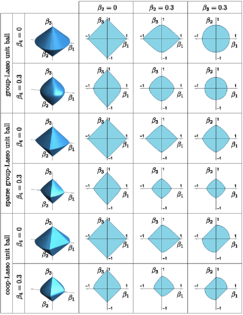
Figure 1: Feasible sets for the coop-Lasso, group-Lasso and sparse group-Lasso penalties. First column: cuts through $(\beta_{1},\beta_{2},\beta_{3})$ at $\beta_{4}=0$ and $\beta_{4}=0.3$: $(\beta_{1},\beta_{2})$ span the horizontal plane and $\beta_{3}$ is on the vertical axis; second and third columns: cuts through $(\beta_{1},\beta_{3})$ at various values of $(\beta_{2},\beta_{4})$; last column: cuts through $(\beta_{1},\beta_{2})$ at various values of $(\beta_{3},\beta_{4})$.

These plots provide some insight into the sparsity pattern that originates from the penalties, since sparsity is related to the singularities of the boundary of the feasible set. First, consider the group-Lasso: the first row illustrates that when $\beta_{4}$ is null its group companion $\beta_{3}$ may also be exactly zero (corners on the boundary at $\beta_{3}=0$), while the second row shows that this event is improbable when $\beta_{4}$ differs from zero (smooth boundary at $\beta_{3}=0$). The second and third columns display the same type of relationships within $\mathcal{G}_{1}$ between $\beta_{2}$ and $\beta_{1}$, which are expected due to the symmetries of the unit ball. The last column displays $\ell_{2}$ balls, which characterize the within-groups feasibility subsets, showing that once a group is activated, all its members will be nonzero.

Now, consider the sparse group-norm: the combination of the group and Lasso penalties has uniformly shrunk the feasible set toward the Lasso $\ell_{1}$ unit ball, thus creating new edges that provide a chance to zero any parameter in any situation, with an elastic-net-like penalty [Zou and Hastie (2005)] within and between groups. The comparison of the last two columns illustrates that the differentiation between the within-group and between group penalties is less marked than for the group-Lasso.

Finally, consider the coop-norm: compared to the group-norm, there are also additional discontinuities resulting in new edges on the 3-D plots. While the sparse group-Lasso edges where created by a uniform shrinking toward the $\ell_{1}$ unit ball, the coop-Lasso new edges result from slicing the group-Lasso unit ball, depriving sign-incoherent orthants from some of the group-Lasso feasible solutions ($\|\bm{\beta}\|_{\mathrm{coop}}>\|\bm{\beta}\|_{\mathrm{group}}$ in these regions). Note that, in general, there are less new edges than with the sparse group-Lasso, since the new opportunities to zero some coefficients are limited to the case where the group-Lasso would have allowed a solution with opposite signs within a group. The crucial difference with the group and sparse group-Lasso is the loss of the axial symmetry when some variables are nonzero: decoupling the positive and negative parts of the regression coefficients favors solutions where signs match within a group. Slicing of the unit group-norm ball does not affect the positive and negative orthants, but large areas corresponding to sign mismatches have been peeled off, as best seen on the last column, which also illustrates the strong differentiation between within-group and between-group penalties.

Before stating the optimality conditions for problem (5), we introduce some notation related to the sparsity pattern of parameters, which will be required to express the necessary and sufficient condition for optimality. First, we recall that the unknown vector of parameters $\bm{\beta}^{\star}$ is typically sparse; its support is denoted $\mathcal{S}=\{j,\bm{\beta}_{j}^{\star}\neq 0\}$ and $\mathcal{S}^{c}=\{j,\bm{\beta}_{j}^{\star}=0\}$ is the complementary set of true zeros. Once the problem has been supplied with a group structure, we define $\mathcal{S}_{k}=\mathcal{S}\cap\mathcal{G}_{k}$ and $\mathcal{S}_{k}^{c}=\mathcal{S}^{c}\cap\mathcal{G}_{k}$ as the sets of relevant, respectively irrelevant, predictors within group $k$, for all $k=1,\ldots,K$. Similar notation $\mathcal{S}(\bm{\beta})$, $\mathcal{S}_{k}(\bm{\beta})$ and $\mathcal{S}_{k}^{c}(\bm{\beta})$ is defined for an arbitrary vector $\bm{\beta}\in\mathbb{R}^{p}$. Furthermore, for clarity and brevity, we introduce the functions $\{\bm{\varphi}_{j}\}_{j=1}^{p}$, which return the componentwise positive or negative part of a vector according to the sign of its $j$th element, that is, $\forall k\in\{1,\ldots,K\},\forall j\in\mathcal{G}_{k},\forall\mathbf{v}\in\mathbb{R}^{p_{k}},$

$$\bm{\varphi}_{j}(\mathbf{v})=(\operatorname{sign}(v_{j})\mathbf{v})^{+}=\cases{\displaystyle\mathbf{0},&\quad if $v_{j}=0$,\cr\displaystyle\mathbf{v}^{+},&\quad if $v_{j}>0$,\cr\displaystyle\mathbf{v}^{-},&\quad if $v_{j}<0$.}$$ (6)

Optimality conditions. The objective function $L$ in (5) is continuous and coercive, thus problem (5) admits at least one minimum. If $\mathbf{X}$ has rank $p$, then the minimum is unique since $L$ is strictly convex. Furthermore, $L$ is smooth, except at some locations with zero coefficients, due to the singularities of the coop-norm. Since $L$ is convex, a necessary and sufficient condition for the optimality of $\bm{\beta}$ is that the null vector $\mathbf{0}$ belongs to the subdifferential of $L$ whose expression is provided in the following lemma.

Lemma 1

For all $\bm{\beta}\in\mathbb{R}^{p}$, the subdifferential of the objective function of problem (5) is

$$\partial_{\bm{\beta}}L(\bm{\beta})=\{\mathbf{v}\in\mathbb{R}^{p}\dvtx\mathbf{v}=\mathbf{X}^{\intercal}(\mathbf{X}\bm{\beta}-\mathbf{y})+\lambda\bm{\theta}\},$$ (7)

where $\bm{\theta}\in\mathbb{R}^{p}$ is any vector belonging to the subdifferential of the coop-norm, that is,

$$\forall k \in \{1,\ldots,K\},\forall j\in\mathcal{S}_{k}(\bm{\beta})\qquad\theta_{j}=\frac{w_{k}\beta_{j}}{\|\bm{\varphi}_{j}(\bm{\beta}_{\mathcal{G}_{k}})\|},$$ (8a)

$$\forall k \in \{1,\ldots,K\},\forall j\in\mathcal{S}_{k}^{c}(\bm{\beta})\qquad\|\bm{\varphi}_{j}(\bm{\theta}_{\mathcal{G}_{k}})\|\leq w_{k}.$$ (8b)

The following optimality conditions, which result directly from Lemma 1, are an essential building block of the algorithm we propose to compute the coop-Lasso estimate. They also provide an important basis for showing the consistency results.

Theorem 1

Problem (5) admits at least one solution, which is unique if $\mathbf{X}$ has rank $p$. All critical points $\bm{\beta}$ of the objective function $L$ verifying the following conditions are global minima:

$$\forall k \in \{1,\ldots,K\},\forall j\in\mathcal{S}_{k}(\bm{\beta})\qquad\mathbf{x}^{\intercal}_{j}(\mathbf{X}\bm{\beta}-\mathbf{y})+\frac{\lambda w_{k}\beta_{j}}{\|\bm{\varphi}_{j}(\bm{\beta}_{\mathcal{G}_{k}})\|}=0,$$ (9a)

$$\forall k \in \{1,\ldots,K\},\forall j\in\mathcal{S}_{k}^{c}(\bm{\beta})\qquad\bigl{\|}\bm{\varphi}_{j}\bigl{(}(\mathbf{X}_{\centerdot\mathcal{G}_{k}})^{\intercal}(\mathbf{X}\bm{\beta}-\mathbf{y})\bigr{)}\bigr{\|}\leq\lambda w_{k},$$ (9b)

where $\mathbf{X}_{\centerdot\mathcal{G}_{k}}$ is the submatrix of $\mathbf{X}$ with all rows and columns indexed by $\mathcal{G}_{k}$.

Note here an important distinction compared to the group-Lasso, where the optimality conditions are expressed solely according to the groups $\mathcal{G}_{k}$ [see, e.g., Roth and Fischer (2008)]. Hence, while the sparsity pattern of the solution is strongly constrained by the predefined group structure in the group-Lasso, deviations from this structure are possible for the coop-Lasso. The asymptotic analysis of Section 3 confirms that exact support recovery is possible even when the support of $\bm{\beta}^{\star}$ cannot be expressed as a simple union of groups, provided the groups intersecting the true support are sign-coherent.

2.2 Algorithm

The efficient approaches developed for the Lasso take advantage of the sparsity of the solution by solving a series of small linear systems, whose sizes are incrementally increased/decreased [Osborne, Presnell and Turlach (2000)]. This approach was pursued for the group-Lasso [Roth and Fischer (2008)] and we proposed an algorithm in the same vein for the coop-Lasso in the framework of multiple network inference [Chiquet, Grandvalet and Ambroise (2011)]. We provide here a more detailed description of the latter in the specific context of linear regression.

The algorithm starts from a sparse initial guess, say, $\bm{\beta}=0$, and iterates two steps: [2.]

The first step solves problem (5) with respect to $\bm{\beta}_{\mathcal{A}}$, the subset of “active” variables, currently identified as being nonzero. At this stage the current feasible set is restricted to the orthants where the gradient of the coop-norm has no discontinuities: the optimization problem is thus smooth. One or more variables may then be declared inactive if the current optimal $\bm{\beta}_{\mathcal{A}}$ reaches the boundary of the current feasible set.

The second step assesses the completeness of the set $\mathcal{A}$, by checking the optimality conditions with respect to inactive variables. We add a group that violates these conditions. In our implementation, we pick the one that most violates the optimality condition, since this strategy has been observed to require few changes in the active set. When no such violation exists, the current solution is optimal.

        Init. Start from a feasible $\bm{\beta}\leftarrow\bm{\beta}^{0}$ $\displaystyle\mathcal{A}_{+}$ $\displaystyle\leftarrow$ $\displaystyle\{j\in\mathcal{G}_{k}\dvtx\|\bm{\beta}_{\mathcal{G}_{k}}^{+}\|>0,k=1,\ldots,K\},$ $\displaystyle\mathcal{A}_{-}$ $\displaystyle\leftarrow$ $\displaystyle\{j\in\mathcal{G}_{k}\dvtx\|\bm{\beta}_{\mathcal{G}_{k}}^{-}\|>0,k=1,\ldots,K\}.$ Step 2.2 On $\mathcal{A}\leftarrow\mathcal{A}_{+}\cup\mathcal{A}_{-}$, find a solution to the smooth problem $\displaystyle\bm{\beta}_{\mathcal{A}}\leftarrow\operatorname{\arg\min}\limits_{\mathbf{v}\in\mathbb{R}^{|\mathcal{A}|}}\frac{1}{2}\|\mathbf{y}-\mathbf{X}_{\centerdot\mathcal{A}}\mathbf{v}\|^{2}+\lambda\|\mathbf{v}\|_{\mathrm{coop}}$ $\displaystyle\eqntext{\mbox{s.t. }\cases{\displaystyle v_{j}\geq 0,&\quad if $j\in\mathcal{A}_{+}\cap\mathcal{A}_{-}^{c}$,\cr\displaystyle v_{j}\leq 0,&\quad if $j\in\mathcal{A}_{-}\cap\mathcal{A}_{+}^{c}$,}}$ (10) where $\mathcal{A}_{-}^{c}$ and $\mathcal{A}_{+}^{c}$ are the complementary sets of $\mathcal{A}_{-}$ and $\mathcal{A}_{+}$, respectively.

Identify groups inactivated during optimization

$$\mathcal{A}_{+} \leftarrow \mathcal{A}_{+}\bigm{\backslash}\Bigl{\{}j\in\mathcal{G}_{k}\subseteq\mathcal{A}_{+}\dvtx\|\bm{\beta}_{\mathcal{G}_{k}}^{+}\|=0$$

$$\hphantom{\mathcal{A}_{+}\setminus\Bigl{\{}}\mbox{and }\min_{\mathbf{v}\in\partial_{\bm{\beta}_{\mathcal{G}_{k}}}L(\bm{\beta})}\|\mathbf{v^{-}}\|=0,k=1,\ldots,K\Bigr{\}},$$

$$\mathcal{A}_{-} \leftarrow \mathcal{A}_{-}\bigm{\backslash}\Bigl{\{}j\in\mathcal{G}_{k}\subseteq\mathcal{A}_{-}\dvtx\|\bm{\beta}_{\mathcal{G}_{k}}^{-}\|=0$$

$$\hphantom{\mathcal{A}_{-}\bigm{\backslash}\Bigl{\{}}\mbox{and }\min_{\mathbf{v}\in\partial_{\bm{\beta}_{\mathcal{G}_{k}}}L(\bm{\beta})}\|\mathbf{v^{+}}\|=0,k=1,\ldots,K\Bigr{\}}.$$

Step 2.2  Identify the greatest violation of optimality conditions:

$$g^{k}_{+} \leftarrow \min_{\mathbf{v}\in\partial_{\bm{\beta}_{\mathcal{G}_{k}}}L(\bm{\beta})}\|\mathbf{v^{+}}\|,\qquad q\leftarrow\operatorname{\arg\max}\limits_{k}g^{k}_{+},$$

$$g^{k}_{-} \leftarrow \min_{\mathbf{v}\in\partial_{\bm{\beta}_{\mathcal{G}_{k}}}L(\bm{\beta})}\|\mathbf{v^{-}}\|,\qquad r\leftarrow\operatorname{\arg\max}\limits_{k}g^{k}_{-}$$

if $\max(g^{q}_{+},g^{r}_{-})=0$ then  Stop and return $\bm{\beta}$, which is optimal else  if $g^{q}_{+}>g^{r}_{-}$ then $\mathcal{A}_{-}\leftarrow\mathcal{A}_{-}\cup\mathcal{G}_{q}$ else  $\mathcal{A}_{+}\leftarrow\mathcal{A}_{+}\cup\mathcal{G}_{r}$ Repeat Steps 1 and 2 until convergence  

Algorithm 1 Coop-Lasso fitting algorithm

These two steps outline the algorithm, which is detailed in more technical terms in Algorithm 1. The principle is readily applied to any generalized linear model by simply defining the appropriate objective function $L$. In our current implementation (a pre-release of our R-package scoop is available at http://stat.genopole.cnrs.fr/logiciels/scoop) the linear and logistic regression models are implemented using either Broyden–Fletcher–Goldfarb–Shanno (BFGS) quasi-Newton updates with box constraints, or proximal methods [Beck and Teboulle (2009)] to solve the smooth optimization problem in Step 2.2.

Finally, note that to compute a series of solutions along the regularization path for problem (5), we simply choose a series of penalties $\lambda^{1}=\lambda_{\mathrm{max}}>\cdots>\lambda^{l}>\cdots>\lambda^{L}=\lambda_{\mathrm{min}}\geq 0$ such that $\hat{\bm{\beta}}{}^{\mathrm{coop}}(\lambda_{\mathrm{max}})=\mathbf{0}$, that is,

$$\lambda_{\mathrm{max}}=\max_{k\in\{1,\ldots,K\}}\max_{j\in\mathcal{G}_{k}}\frac{1}{w_{k}}\|\bm{\varphi}_{j}((\mathbf{X}_{\centerdot\mathcal{G}_{k}})^{\intercal}\mathbf{y})\|.$$

We then use the usual warm start strategy, where the feasible initial guess for $\hat{\bm{\beta}}{}^{\mathrm{coop}}(\lambda^{l})$, the coop-Lasso estimate with penalty parameter $\lambda^{l}$, is initialized with $\hat{\bm{\beta}}{}^{\mathrm{coop}}(\lambda^{l-1})$.

2.3 Orthonormal design case

The orthonormal design case, where$\mathbf{X}^{\intercal}\mathbf{X}=\mathbf{I}_{p}$, has been providing useful insights for penalization techniques regarding the effects of shrinkage. Indeed, in this particular case, most usual shrinkage estimators can be expressed in closed-form as functions of the ordinary least squares (OLS) estimate. These expressions pave the way for the derivation of approximations of the degrees of freedom [Tibshirani (1996); Yuan and Lin (2006) and Section 4], which may be convenient for model selection in the absence of exact formulae.

In the orthonormal setting, for any $\beta_{j}$, we have $\mathbf{x}_{j}^{\intercal}(\mathbf{X}\bm{\beta}-\mathbf{y})=\beta_{j}-\hat{\beta}_{j}^{\mathrm{ols}}$. The optimality conditions (9a) and (9b) can then be written as

$$\forall k\in\{1,\ldots,K\},\forall j\in\mathcal{G}_{k}\qquad\hat{\beta}_{j}^{\mathrm{coop}}=\biggl{(}1-\frac{\lambda w_{k}}{\|\bm{\varphi}_{j}(\hat{\bm{\beta}}{}^{\mathrm{ols}}_{\mathcal{G}_{k}})\|}\biggr{)}^{+}\hat{\beta}_{j}^{\mathrm{ols}}.$$ (11)

For reference, we recall the solution to the group-Lasso [Yuan and Lin (2006)] in the same condition

$$\forall k\in\{1,\ldots,K\},\forall j\in\mathcal{G}_{k}\qquad\hat{\beta}_{j}^{\mathrm{group}}=\biggl{(}1-\frac{\lambda w_{k}}{\|\hat{\bm{\beta}}{}^{\mathrm{ols}}_{\mathcal{G}_{k}}\|}\biggr{)}^{+}\hat{\beta}_{j}^{\mathrm{ols}},$$ (12)

while the Lasso solution [Tibshirani (1996)] is

$$\forall j\in\{1,\ldots,p\}\qquad\hat{\beta}_{j}^{\mathrm{lasso}}=\biggl{(}1-\frac{\lambda}{|\hat{\beta}_{j}^{\mathrm{ols}}|}\biggr{)}^{+}\hat{\beta}_{j}^{\mathrm{ols}}.$$ (13)

Equations (11)–(13) reveal strong commonalities. First, the coefficients of these shrinkage estimators are of the sign of the OLS estimates. Second, the norm used in the penalty defines a region where small OLS coefficients are shrunk to zero, while large ones are shrunk inversely proportional to this norm. Finally, by grouping the terms corresponding to one group in equations (11)–(12), a uniform translation effect, analogous to the one observed for the Lasso, comes into view:

$$\displaystyle\forall k\in\{1,\ldots,K\},\forall j\in\mathcal{G}_{k}\qquad\|\bm{\varphi}_{j}(\hat{\bm{\beta}}{}^{\mathrm{coop}}_{\mathcal{G}_{k}})\|=\bigl{(}\|\bm{\varphi}_{j}(\hat{\bm{\beta}}{}^{\mathrm{ols}}_{\mathcal{G}_{k}})\|-\lambda w_{k}\bigr{)}^{+},$$

$$\displaystyle\forall k\in\{1,\ldots,K\}\qquad\|\hat{\bm{\beta}}{}^{\mathrm{group}}_{\mathcal{G}_{k}}\|=(\|\hat{\bm{\beta}}{}^{\mathrm{ols}}_{\mathcal{G}_{k}}\|-\lambda w_{k})^{+},$$ (14)

$$\displaystyle\forall j\in\{1,\ldots,p\}\qquad|\hat{\beta}_{j}^{\mathrm{lasso}}|=(|\hat{\beta}_{j}^{\mathrm{ols}}|-\lambda w_{k})^{+}.$$

The group-Lasso (12) differs primarily from the Lasso (13) owing to the common penalty ${\lambda w_{k}}/{\|\hat{\bm{\beta}}{}^{\mathrm{ols}}_{\mathcal{G}_{k}}\|}$ for all the coefficients belonging to group $k$. The magnitude of shrinkage is determined by all within-group OLS coefficients, and is thus radically different from a ridge regression penalty in this regard. For the coop-Lasso estimator (11), two penalties possibly apply to group $k$, for the positive and the negative OLS coefficients, respectively. If all within-group OLS coefficients are of the same sign, coop-Lasso is identical to group-Lasso; if some signs disagree, the magnitude of the penalty only depends on the within-group OLS coefficients with an identical sign. In the extreme case where exactly one OLS coefficient is positive/negative, the coop-penalty is identical to a Lasso penalty on this coefficient.

Note that such a simple analytical formulation is not available for the sparse group-Lasso estimate $\hat{\bm{\beta}}{}^{\mathrm{sgl}}$, but an expression can be obtained by chaining two simple shrinkage operations. Introducing an intermediate solution $\tilde{\bm{\beta}}{}^{\mathrm{sgl}}$, we have, $\forall k\in\{1,\ldots,K\}$ and $\forall j\in\mathcal{G}_{k},$

$$\qquad\hat{\beta}_{j}^{\mathrm{sgl}}=\biggl{(}1-\frac{\lambda(1-\alpha)w_{k}}{\|\tilde{\bm{\beta}}{}^{\mathrm{sgl}}_{\mathcal{G}_{k}}\|}\biggr{)}^{+}\tilde{\beta}{}^{\mathrm{sgl}}_{j}\qquad\mbox{where }\tilde{\beta}{}^{\mathrm{sgl}}_{j}=\biggl{(}1-\frac{\lambda\alpha}{|\hat{\beta}_{j}^{\mathrm{ols}}|}\biggr{)}^{+}\hat{\beta}_{j}^{\mathrm{ols}}.$$ (15)

The intermediate solution $\tilde{\bm{\beta}}{}^{\mathrm{sgl}}$ is the Lasso estimator with penalty parameter $\lambda\alpha$, which acts as the OLS estimate for a group-Lasso of parameter $\lambda(1-\alpha)$.

Figure 2 provides a visual representation of equations (11)–(13) and (15) for a group with two components, say, $\mathcal{G}_{k}=\{1,2\}$.

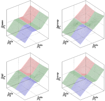
Figure 2: Lasso, group, sparse group and coop Lasso coefficient estimates, for a group with 2 elements $\mathcal{G}_{k}=\{1,2\}$, as a function of the OLS coefficients. The colors emphasize the positive and negative quadrants of the $(\hat{\beta}{}^{\mathrm{ols}}_{1},\hat{\beta}{}^{\mathrm{ols}}_{2})$ plane, with red and blue, respectively.

We plot $\hat{\beta}_{1}^{\mathrm{lasso}},\hat{\beta}_{1}^{\mathrm{group}},\hat{\beta}_{1}^{\mathrm{sgl}}$ and $\hat{\beta}_{1}^{\mathrm{coop}}$ as functions of $(\hat{\beta}_{1}^{\mathrm{ols}},\hat{\beta}_{2}^{\mathrm{ols}})$. Top-left, the Lasso translates the $\hat{\beta}_{1}^{\mathrm{ols}}$ coefficient toward zero, eventually truncating them at zero, regardless of $\hat{\beta}_{2}^{\mathrm{ols}}$: there is no interaction between coefficients. The group-Lasso, top-right, has a nonlinear shrinking behavior (quite different from the Lasso or ridge penalties in this respect) and sets $\hat{\beta}_{1}^{\mathrm{group}}$ to zero within a Euclidean ball centered at zero. The sparse group-Lasso, bottom-left, is a hybrid of Lasso and group-Lasso, whose shrinking behavior lies between its two ancestors. Bottom-right, the coop-Lasso appears as another form of cross-breed, identical to the group-Lasso in the positive and negative quadrants, and identical to the Lasso when the signs of the OLS coefficients mismatch. For groups with more than two components, intermediate solutions would be possible. This behavior is shown to allow for some flexibility with respect to the predefined group structure in the following consistency analysis.

3 Consistency

Beyond its sanity-check value, a consistency analysis brings along an appreciation of the strengths and limitations of an estimation scheme. Here we concentrate on the estimation of the support of the parameter vector, that is, the position of its zero entries. Our proof technique is drawn from the previous works on the Lasso [Yuan and Lin (2007)] and the group-Lasso [Bach (2008)].

In this type of analysis, some assumptions on the joint distribution of $(X,Y)$ are required to guarantee the convergence of empirical covariances. For the sake of simplicity and coherence, we keep assuming that data are centered so that we have zero mean random variables and $\bm{\Psi}=\mathbb{E}[XX^{\intercal}]$ is the covariance matrix of $X$: [(A2)]

$X$ and $Y$ have finite 4th order moments $\mathbb{E}[\|X\|^{4}]<\infty$, $\mathbb{E}[Y^{4}]<\infty$.

The covariance matrix $\bm{\Psi}=\mathbb{E}[XX^{\intercal}]\in\mathbb{R}^{p\times p}$ is invertible.

In addition to these standard technical assumptions, we need a more specific one, substantially avoiding situations where the coop-Lasso will almost never recover the true support: [(A3)]

All sign-incoherent groups are included in the true support: $\forall k\in\{1,\ldots,K\}$, if $\|(\bm{\beta}_{\mathcal{G}_{k}}^{\star})^{+}\|>0$ and $\|(\bm{\beta}_{\mathcal{G}_{k}}^{\star})^{-}\|>0$, then $\forall j\in\mathcal{G}_{k}$, $\bm{\beta}^{\star}_{j}\neq 0$. Note that this latter assumption is less stringent than the one required for the group-Lasso since it does not require that each group of variables should either be included in or excluded from the support. For the coop-Lasso, sign-coherent groups may intersect the support.

The spurious relationships that may arise from confounding variables are controlled by the so-called strong irrepresentable condition, which guarantees support recovery for the Lasso [Yuan and Lin (2007)] and the group-Lasso [Bach (2008)]. We now introduce suitable variants of these conditions for the coop-Lasso. They result in two assumptions: a general one, on the magnitude of correlations between relevant and irrelevant variables, and a more specific one for groups which intersect the support, on the sign of correlations. These conditions will be expressed in a compact vectorial form using the diagonal weighting matrix $\mathbf{D}(\bm{\beta})$ such that,

$$\forall k\in\{1,\ldots,K\},\forall j\in\mathcal{S}_{k}(\bm{\beta})\qquad(\mathbf{D}(\bm{\beta}))_{jj}=w_{k}\|\bm{\varphi}_{j}(\bm{\beta}_{\mathcal{G}_{k}})\|^{-1}.$$ (16)

[(A4)]

For every group $\mathcal{G}_{k}$ including at least one null coefficient (i.e., such that $\beta^{\star}_{j}=0$ for some $j\in\mathcal{G}_{k}$ or, equivalently, $\mathcal{S}^{c}_{k}\neq\varnothing$), there exists $\eta>0$ such that

$$\frac{1}{w_{k}}\max(\|(\bm{\Psi}_{\mathcal{S}_{k}^{c}\mathcal{S}}\bm{\Psi}_{\mathcal{S}\mathcal{S}}^{-1}\mathbf{D}(\bm{\beta}^{\star}_{\mathcal{S}})\bm{\beta}^{\star}_{\mathcal{S}})^{+}\|,\|(\bm{\Psi}_{\mathcal{S}_{k}^{c}\mathcal{S}}\bm{\Psi}_{\mathcal{S}\mathcal{S}}^{-1}\mathbf{D}(\bm{\beta}^{\star}_{\mathcal{S}})\bm{\beta}^{\star}_{\mathcal{S}})^{-}\|)\leq 1-\eta,$$ (17)

where $\bm{\Psi}_{\cal{ST}}$ is the submatrix of $\bm{\Psi}$ with lines and columns respectively indexed by $\cal{S}$ and $\cal{T}$. [(A5)]

For every group $\mathcal{G}_{k}$ intersecting the support and including either positive or negative coefficients, letting $\nu_{k}$ be the sign of these coefficients [$\nu_{k}=1$ if $\|(\bm{\beta}_{\mathcal{G}_{k}}^{\star})^{+}\|>0$ and $\nu_{k}=-1$ if $\|(\bm{\beta}_{\mathcal{G}_{k}}^{\star})^{-}\|>0$], the following inequalities should hold:

$$\nu_{k}\bm{\Psi}_{\mathcal{S}^{c}_{k}\mathcal{S}}\bm{\Psi}_{\mathcal{S}\mathcal{S}}^{-1}\mathbf{D}(\bm{\beta}^{\star}_{\mathcal{S}})\bm{\beta}^{\star}_{\mathcal{S}}\preceq\mathbf{0},$$ (18)

where $\preceq$ denotes componentwise inequality. Note that the irrepresentable condition for the group-Lasso only considers correlations between groups included and excluded from the support. It is otherwise similar to (17), except that the elements of the weighting matrix $\mathbf{D}$ are $w_{k}\|\bm{\beta}_{\mathcal{G}_{k}}\|^{-1}$ and that the $\ell_{2}$ norm replaces $\max(\|(\cdot)^{+}\|,\|(\cdot)^{-}\|)$.

We now have all the components for stating the coop-Lasso consistency theorem, which will consider the following normalized (equivalent) form of the optimization problem (5) to allow a direct comparison with the known similar results previously stated for the Lasso and group-Lasso [Yuan and Lin (2007); Bach (2008)]:

$$\hat{\bm{\beta}}{}^{\mathrm{coop}}_{n}=\operatorname{\arg\min}\limits_{\bm{\beta}\in\mathbb{R}^{p}}\frac{1}{2n}\|\mathbf{y}-\mathbf{X}\bm{\beta}\|^{2}+\lambda_{n}\|\bm{\beta}\|_{\mathrm{coop}},$$ (19)

where $\lambda_{n}=\lambda/n$.

Theorem 2

If assumptions (A1)–(A5) are satisfied, the coop-Lasso estimator is asymptotically unbiased and has the property of exact support recovery:

$$\hat{\bm{\beta}}{}^{\mathrm{coop}}_{n}\stackrel{{\scriptstyle P}}{{\longrightarrow}}\bm{\beta}^{\star}\quad\mbox{and}\quad\mathbb{P}\bigl{(}\mathcal{S}(\hat{\bm{\beta}}{}^{\mathrm{coop}}_{n})=\mathcal{S}\bigr{)}\rightarrow 1,$$ (20)

for every sequence $\lambda_{n}$ such that $\lambda_{n}=\lambda_{0}n^{-\gamma},\gamma\in(0,1/2)$.

Compared to the group-Lasso, the consistency of support recovery for the coop-Lasso differs primarily regarding possible intersection (besides inclusion and exclusion) between groups and support. This additional flexibility applies to every sign-coherent group. Even if the support is the union of groups, when all groups are sign-coherent, the coop-Lasso has still an edge on group-Lasso since the irrepresentable condition (17) is weaker. Indeed, the norm in (17) is dominated by the $\ell_{2}$ norm used for the group-Lasso. The next paragraph illustrates that this difference can have remarkable outcomes. Finally, when the support is the union of groups comprising sign-incoherent ones, there is no systematic advantage in favor of one or the other method. While the norm used by the coop-Lasso is dominated by the norm used by the group-Lasso, the weighting matrix $\mathbf{D}$ has smaller entries for the latter.

Illustration. We generate data from the regression model (1), with $\bm{\beta}^{\star}=(1,1,-1,-1,0,0,0,0)$, equipped with the group structure $\{\mathcal{G}_{k}\}_{k=1}^{4}=\{\{1,2\},\allowbreak\{3,4\},\{5,6\},\{7,8\}\}$. The vector $X$ is generated as a centered Gaussian random vector whose covariance matrix $\bm{\Psi}$ is chosen so that the irrepresentable conditions hold for the coop-Lasso, but not for the group-Lasso, which, we recall, are more demanding for the current situation, with sign-coherent groups. The random error $\varepsilon$ follows a centered Gaussian distribution with standard deviation $\sigma=0.1$, inducing a very high signal to noise ratio ($R^{2}=0.99$ on average), so that asymptotics provide a realistic view of the finite sample situation.

We generated 1000 samples of size $n=20$ from the described model, and computed the corresponding 1000 regularization paths for the group-Lasso, sparse group-Lasso and coop-Lasso. Figure 3 reports the 50% coverage intervals (lower and upper quartiles) along the regularization paths. In this setup, the sparse group-Lasso behaves as the group-Lasso, leading to nearly identical graphs.

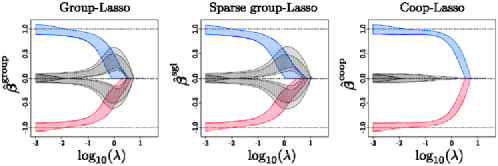
Figure 3: 50% coverage intervals for the group (left), sparse group (center) and (right) Lasso estimated coefficients along regularization paths: coefficients from the support of $\bm{\beta}^{\star}$ are marked by colored horizontal stripes and the other ones by gray vertical stripes.

Estimation is difficult in this small sample problem ($n=20,p=8$), and the two versions of the group-Lasso, which first select the wrong covariates, never reach the situation where they would have a decisive advantage upon OLS, while the coop-Lasso immediately selects the right covariates, whose coefficients steadily dominate the irrelevant ones. Model selection is also difficult, and the BIC criteria provided in Section 4 select often the OLS model (in about $10\%$ and $50\%$ of cases for the coop-Lasso and the group-Lasso, respectively). The average root mean square error on parameters is of order $10^{-1}$ for all methods, with a slight edge for the coop-Lasso. The sign error is much more contrasted: $31\%$ for the coop-Lasso vs. $46\%$ for the group-Lasso, not far better than the $50\%$ of OLS.

4 Model selection

Model selection amounts here to choosing the penalization parameter $\lambda$, which restricts the size of the estimate $\hat{\bm{\beta}}(\lambda)$. Trial values $\{\lambda_{\mathrm{min}},\ldots,\lambda_{\mathrm{max}}\}$ define the set of models we have to choose from along the regularization path. The process aims at picking the model with minimum prediction error, or the one closest to the model from which data have been generated, assuming the model is correct, that is, equation (1) holds. Here “closest” is typically measured by a distance between $\hat{\bm{\beta}}$ and $\bm{\beta}^{\star}$, either based on the value of the coefficients or on their support (true model selection), and sometimes also on the sign correctness of each nonzero entry.

Among the prerequisite for the selection process to be valid, the previous consistency analysis comes up with suitable orders of magnitude for the penalty parameter $\lambda$. However, it does not provide a proper value to be plugged in (5) and the practice is to use data driven approaches for selecting an appropriate penalty parameter.

Cross-validation is a recommended option [Hesterberg et al. (2008)] when looking for the model minimizing the prediction error, but it is slow and not well suited to select the model closest to the true one. Analytical criteria provide a faster way to perform model selection and, though the information criteria AIC and BIC rely on asymptotic derivations, they often offer good practical performances. The BIC and AIC criteria for the Lasso [Zou, Hastie and Tibshirani (2007)] and group-Lasso [Yuan and Lin (2006)] have been defined through the effective degrees of freedom:

$$\mathrm{AIC}(\lambda) = \frac{\|\mathbf{y}-\hat{\mathbf{y}}(\lambda)\|^{2}}{\sigma^{2}}+2\operatorname{df}(\lambda),$$ (21)

$$\mathrm{BIC}(\lambda) = \frac{\|\mathbf{y}-\hat{\mathbf{y}}(\lambda)\|^{2}}{\sigma^{2}}+\log(n)\operatorname{df}(\lambda),$$ (22)

where $\hat{\mathbf{y}}(\lambda)=\mathbf{X}\hat{\bm{\beta}}(\lambda)$ is the vector of predicted values for (5) with penalty parameter $\lambda$, $\sigma^{2}$ is the variance of the zero-mean Gaussian error variable $\varepsilon$ in (1) and $\operatorname{df}(\lambda)$ is the number of degrees of freedom of the selected model. Assuming that equation (1) holds and a differentiability condition on the mapping $\hat{\mathbf{y}}(\lambda)$, Efron (2004), using Stein’s theory of unbiased risk estimate [Stein (1981)], shows that

$$\operatorname{df}(\lambda)\doteq\frac{1}{\sigma^{2}}\sum_{i=1}^{n}\operatorname{cov}(\hat{y}_{i}(\lambda),y_{i})=\mathbb{E}\biggl{[}\operatorname{tr}\biggl{(}\frac{\partial\hat{\mathbf{y}}(\lambda)}{\partial\mathbf{y}}\biggr{)}\biggr{]},$$ (23)

where the expectation is taken with respect to $\mathbf{y}$ or, equivalently, to the noise $\bm{\varepsilon}$. Yuan and Lin (2006) proposed an approximation of the trace term in the right-hand side of (23), which is used to estimate $\operatorname{df}(\lambda)$ for the group-Lasso:

$$\widetilde{\operatorname{df}}_{\mathrm{group}}(\lambda)=\sum_{k=1}^{K}\mathbh{1}\bigl{(}\|\hat{\bm{\beta}}{}^{\mathrm{group}}_{\mathcal{G}_{k}}(\lambda)\|>0\bigr{)}\biggl{(}1+\frac{\|\hat{\bm{\beta}}{}^{\mathrm{group}}_{\mathcal{G}_{k}}(\lambda)\|}{\|\bm{\beta}{}^{\mathrm{ols}}_{\mathcal{G}_{k}}\|}(p_{k}-1)\biggr{)},$$ (24)

where $\mathbh{1}(\cdot)$ is the indicator function and $p_{k}$ is the number of elements in $\mathcal{G}_{k}$. For orthonormal design matrices, (24) is an unbiased estimate of the true degrees of freedom of the group-Lasso and Yuan and Lin (2006) suggest that this approximation is relevant in more general settings, by reporting that “the performance of this approximate $C_{p}$-criterion [directly derived from (24)] is generally comparable with that of fivefold cross-validation and is sometimes better.”

This approximation of $\operatorname{df}(\lambda)$ relies on the OLS estimate and is hence limited to setups where the latter exists and is unique. In particular, the sample size should be larger than the number of predictors ($n\geq p$). To overcome this restriction, we suggest a more general approximation to the degrees of freedom, based on the ridge estimator

$$\hat{\bm{\beta}}{}^{\mathrm{ridge}}(\gamma)=(\mathbf{X}^{\intercal}\mathbf{X}+\gamma\mathbf{I})^{-1}\mathbf{X}^{\intercal}\mathbf{y},$$ (25)

which can be computed even for small sample sizes ($n<p$).

Proposition 1

Consider the coop-Lasso estimator $\hat{\bm{\beta}}{}^{\mathrm{coop}}(\lambda)$ defined by (5). Assuming that data are generated according to model (1), and that $\mathbf{X}$ is orthonormal, the following expression of $\widetilde{\operatorname{df}}_{\mathrm{coop}}(\lambda)$ is an unbiased estimate of $\operatorname{df}(\lambda)$ defined in (23) for the coop-Lasso fit:

$$\widetilde{\operatorname{df}}_{\mathrm{coop}}(\lambda) = \sum_{k=1}^{K}\mathbh{1}\bigl{(}\|(\hat{\bm{\beta}}{}^{\mathrm{coop}}_{\mathcal{G}_{k}}(\lambda))^{+}\|>0\bigr{)}\biggl{(}1+\frac{p^{k}_{+}-1}{1+\gamma}\frac{\|(\hat{\bm{\beta}}{}^{\mathrm{coop}}_{\mathcal{G}_{k}}(\lambda))^{+}\|}{\|(\hat{\bm{\beta}}{}^{\mathrm{ridge}}_{\mathcal{G}_{k}}(\gamma))^{+}\|}\biggr{)}$$

$$\hphantom{\sum_{k=1}^{K}}{}+\mathbh{1}\bigl{(}\|(\hat{\bm{\beta}}{}^{\mathrm{coop}}_{\mathcal{G}_{k}}(\lambda))^{-}\|>0\bigr{)}\biggl{(}1+\frac{p^{k}_{-}-1}{1+\gamma}\frac{\|(\hat{\bm{\beta}}{}^{\mathrm{coop}}_{\mathcal{G}_{k}}(\lambda))^{-}\|}{\|(\hat{\bm{\beta}}{}^{\mathrm{ridge}}_{\mathcal{G}_{k}}(\gamma))^{-}\|}\biggr{)},$$

where $p^{k}_{+}$ and $p^{k}_{-}$ are respectively the number of positive and negative entries in $\hat{\bm{\beta}}{}^{\mathrm{ridge}}_{\mathcal{G}_{k}}(\gamma)$.

Proposition 1 raises a practical issue regarding the choice of a good reference $\hat{\bm{\beta}}{}^{\mathrm{ridge}}(\gamma)$. In our numerous simulations (most of which are not reported here), we did not observe a high sensitivity to $\gamma$, though high values degrade performances. When $\mathbf{X}$ is full rank we use $\gamma=0$ (the OLS estimate) and, correspondingly, a vanishing $\gamma$ (the Moore–Penrose solution) when $\mathbf{X}$ is of smaller rank. More refined strategies are left for future works.

Section 5 illustrates that, even in nonorthonormal settings, plugging expression (1) for the degrees of freedom $\operatorname{df}(\lambda)$ of the coop-Lasso in BIC (22) or AIC (21) provides sensible model selection criteria. As expected, BIC, which is more stringent than AIC, is better at retrieving the sparsity pattern of $\bm{\beta}^{\star}$, while AIC is slightly better regarding prediction error.

5 Simulation study

We report here experimental results in the regression setup, with the linear regression model (1). Our simulation protocol is inspired from the one proposed by Breiman (1995, 1996) to test the nonnegative garrote estimator, which inspired the Lasso.

5.1 Data generation

The structure of $\bm{\beta}^{\star}\in\mathbb{R}^{p}$ is controlled through sparsity at coefficient and group levels. Here we have $p=90$, forming $K=10$ groups of identical size, $p_{k}=9$. All groups of parameters follow the same wave pattern: for $j\in\{1,\ldots,9\}$, $(\bm{\beta}^{\star}_{\mathcal{G}_{k}})_{j}\propto\nu_{k}((h-|5-j|)^{+})^{2}$, where $\nu_{k}\in\{0,1\}$ is a switch at the group level and $h\in\{3,4,5\}$ governs the wave width, that is, the within-group sparsity, with respectively $|\mathcal{S}_{k}|\in\{5,7,9\}$ nonzero coefficients in each group included in the support. The covariates are drawn from a multivariate normal distribution $X\sim\mathcal{N}(\mathbf{0},\bm{\Psi})$ with, for all $(j,j^{\prime})\in\{1,\ldots,p\}^{2}$, covariances $\Psi_{jj^{\prime}}=\rho^{|j-j^{\prime}|}$, where $\rho\in[-1,1]$. Finally, the response is corrupted by an error variable $\varepsilon\sim\mathcal{N}(0,1)$ and the magnitude of the vector of parameters $\bm{\beta}^{\star}$ is chosen to have an $R^{2}$ around $0.75$.

Note that the covariance of the covariates is purposely disconnected from the group structure. This setting may either be considered as unfair to the group methods, or equally adverse for all Lasso-type estimators, in the sense that none of their support recovery conditions are fulfilled when $\rho\neq 0$. Situations more or less advantageous for group methods are then produced thanks to the parameter $h$, which determines how the support of $\bm{\beta}^{\star}$ matches the group structure.

5.2 Results

Model selection is performed with BIC (22) for Lasso, group-Lasso and coop-Lasso. The estimation of the degrees of freedom for the Lasso is the number of nonzero entries in $\hat{\bm{\beta}}{}^{\mathrm{lasso}}(\lambda)$ [Zou, Hastie and Tibshirani (2007)]. As there is no such analytical estimate of the degrees of freedom for the sparse group-Lasso, we tested two alternative model selection strategies: standard five-fold cross-validation (CV), selecting the model with minimum cross-validation error, and the so-called “1-SE rule” [Breiman et al. (1984)], which selects the most constrained model whose cross-validation error is within one standard error of the minimum.

First, we display in Figure 4 an example of the regularization paths obtained for each method for a small training set size ($n=p/2=45$) drawn from the model with three active groups having two zero coefficients each ($|\mathcal{S}_{k}|=7$, $p_{k}=9$) and a moderate positive correlation level ($\rho=0.4$).

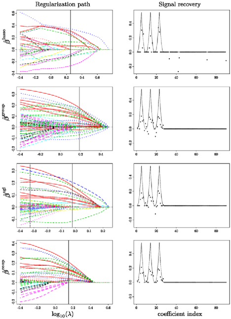
Figure 4: Lasso, group, sparse group and coop Lasso estimates for a training set of size $n=45$ drawn from the generation process of Section 5.1, with 3 active waves out of 10, $|\mathcal{S}_{k}|/p_{k}=7/9$ and $\rho=0.4$. Left: regularization paths, where each line type/color represents a group of parameters and the plain vertical line marks the model selected by the 1-SE rule for sparse group-Lasso and BIC otherwise; right: true signal (dotted line) and estimated parameters for the selected model (filled circles).

As expected, the nonzero coefficients appear one at a time along the Lasso regularization path and groupwise for the other methods, which detect the relevant groups early, with some coefficients kept to zero for the sparse group-Lasso and the coop-Lasso. The sparse group-Lasso is qualitatively intermediate between the group-Lasso and the coop-Lasso, setting many parameters to zero, but keeping a few negative coefficients in the solution. The coefficients of the model estimated by BIC or the 1-SE rule are displayed on the right of each path. The Lasso estimate includes some nonzero coefficients from irrelevant groups, but is otherwise quite conservative, excluding many nonzero parameters from its support. This conservative trend is also observed for the group methods, which exclude all irrelevant groups. The three group estimates mostly agree on truly important coefficients, and differ in the treatment of the spurious negative values that are frequent for group-Lasso, rarer for sparse group-Lasso and do not occur for coop-Lasso.

=330pt Lasso Group Sparse-cv Sparse-1-se Coop Scenario RMSE ($\times 10^{3}$) $|\mathcal{S}_{k}|=5$ $n=45$ 87.1 (0.5) 95.0 (0.5) 82.5 (0.5) 88.1 (0.6) 84.2 (0.5) $n=180$ 43.7 (0.2) 49.1 (0.2) 41.7 (0.2) 44.9 (0.2) 43.5 (0.2) $n=450$ 28.8 (0.1) 33.4 (0.1) 27.2 (0.1) 30.9 (0.1) 29.4 (0.1) $|\mathcal{S}_{k}|=7$ $n=45$ 93.0 (0.5) 85.8 (0.5) 79.7 (0.4) 83.6 (0.5) 76.8 (0.5) $n=180$ 48.4 (0.2) 44.5 (0.2) 42.2 (0.2) 43.7 (0.2) 40.4 (0.2) $n=450$ 31.8 (0.1) 30.3 (0.1) 27.7 (0.1) 30.0 (0.1) 27.6 (0.1) $|\mathcal{S}_{k}|=9$ $n=45$ 99.2 (0.4) 82.0 (0.5) 81.0 (0.4) 83.2 (0.5) 73.7 (0.5) $n=180$ 52.5 (0.2) 41.9 (0.2) 43.3 (0.2) 43.8 (0.2) 39.0 (0.2) $n=450$ 34.1 (0.1) 28.7 (0.1) 28.8 (0.1) 30.6 (0.1) 27.1 (0.1) Scenario Mean sign error ($\%$) $|\mathcal{S}_{k}|=5$ $n=45$ 13.8 (0.1) 18.3 (0.2) 36.7 (0.4) 16.9 (0.3) 13.3 (0.2) $n=180$ 08.4 (0.1) 19.3 (0.2) 36.1 (0.4) 10.7 (0.2) 13.0 (0.2) $n=450$ 06.1 (0.1) 16.7 (0.2) 35.5 (0.4) 07.1 (0.2) 10.3 (0.2) $|\mathcal{S}_{k}|=7$ $n=45$ 18.9 (0.1) 12.9 (0.2) 34.6 (0.4) 16.8 (0.3) 10.1 (0.2) $n=180$ 11.9 (0.1) 12.7 (0.2) 34.5 (0.4) 10.5 (0.2) 09.8 (0.2) $n=450$ 08.8 (0.1) 10.4 (0.2) 34.9 (0.4) 07.1 (0.2) 07.7 (0.2) $|\mathcal{S}_{k}|=9$ $n=45$ 24.4 (0.1) 08.1 (0.2) 34.2 (0.4) 17.3 (0.3) 07.9 (0.2) $n=180$ 15.3 (0.1) 06.3 (0.2) 33.5 (0.4) 10.0 (0.2) 06.7 (0.2) $n=450$ 11.2 (0.1) 04.3 (0.1) 32.6 (0.4) 06.0 (0.2) 04.5 (0.1)

Table 1: Average errors, with standard deviations, on 1000 simulations from the setup described in Section 5.1. Each scenario differs in the number of observations $n$ and the number of active variables per active group $|\mathcal{S}_{k}|$ ($p_{k}=9$). Sparse-cv and sparse-1-se designate the sparse group-Lasso with $\lambda$ selected by cross-validation and by the 1-SE rule, respectively

Table 1 provides a more objective evaluation of the compared methods, based on the root mean square error (RMSE) and the support recovery (more precisely, recovery of the sign of true parameters); prediction error (not shown) is tightly correlated with RMSE in our setup. Regarding the relative merits of the different methods, we did not observe a crucial role of the number of active groups and the covariate correlation level $\rho$. We report results for a true support comprising 3 groups out of 10 and $\rho=0.4$, with various within-group sparsity and sample size scenarios.

All estimators perform about equally in RMSE, the sparse group-Lasso with CV having a slight advantage over the coop-Lasso when many zero coefficients belong to the active groups, and the coop-Lasso being marginally but significantly better elsewhere.

Regarding support recovery, model selection with CV leads to models overestimating the support of parameters. The 1-SE rule, which slightly harms RMSE, is greatly beneficial in this respect. BIC also performs very well, incurring a very small loss due to model selection compared to the oracle solution picking the model with best support recovery. The Lasso dominates all the groups methods when many zero coefficients belong to the active groups. Elsewhere, group methods (with appropriate model selection criteria) perform systematically significantly better for the small sample sizes. The coop-Lasso ranks first or a close second among group methods in all experimental conditions. It thus appears as the method of choice regarding inference issues when groups conform to the sign-coherence assumption.

5.3 Robustness

The robustness to violations of the sign-coherence assumption is assessed by switching a proportion $P_{\sigma}$ of signs in the vector $\bm{\beta}^{\star}$, otherwise generated as before. The sign of the corresponding covariates are switched accordingly, to ensure that only the coop-Lasso estimators are affected in the process.

Table 2 displays the coop-Lasso RMSE that degrades gradually with the amount of perturbation, becoming eventually worse than the Lasso, except for full groups.

=335pt RMSE ($\bm{\times 10^{3}}$) Mean sign error ($\bm{\%}$) $\bm{P_{\sigma}}$ $\bm{|\mathcal{S}_{k}|=5}$ $\bm{|\mathcal{S}_{k}|=7}$ $\bm{|\mathcal{S}_{k}|=9}$ $\bm{|\mathcal{S}_{k}|=5}$ $\bm{|\mathcal{S}_{k}|=7}$ $\bm{|\mathcal{S}_{k}|=9}$ 0.1 46.9 (0.2) 45.3 (0.2) 45.8 (0.2) 15.3 (0.2) 12.4 (0.2) 08.8 (0.2) 0.2 49.5 (0.3) 48.9 (0.2) 48.7 (0.2) 17.8 (0.2) 14.3 (0.2) 09.8 (0.2) 0.3 51.0 (0.3) 50.4 (0.3) 50.4 (0.2) 19.3 (0.2) 14.8 (0.2) 10.3 (0.2) 0.4 51.6 (0.2) 51.0 (0.2) 50.2 (0.2) 19.7 (0.2) 14.8 (0.2) 09.8 (0.2) 0.5 52.3 (0.3) 51.3 (0.2) 50.8 (0.2) 20.0 (0.2) 14.6 (0.2) 09.3 (0.2)

Table 2: Average errors, with standard deviations, on 1000 simulations from the setup of Table 1 with $n=180$, perturbed by switching a proportion $P_{\sigma}$ of signs in $\bm{\beta}^{\star}$

Regarding sign error, for small proportions of sign flip, the coop-Lasso stays at par with either Lasso or group-Lasso (see Table 1), but it eventually becomes significantly worse than both of them in most situations. Thus, if the sign-coherence assumption is not firmly grounded, either group-Lasso or its sparse version seem to be better options: coop-Lasso only remains a second-best choice when there are less than 10% of sign mismatches within groups.

6 Illustrations on real data

This section illustrates the applicability of the coop-Lasso on two types of predictors, that is, categorical and continuous covariates. The first proposal may be widely applied to ordered categorical variables; the second one is specific to microarray data, but should apply more generally when groups of variables are produced by clustering.

In the first application, each group is formed by a set of variables coding an ordered categorical variable. Ordinal data are often processed either by omitting the order property, treating them as nominal, or by replacing each level with a prescribed value, treating them as quantitative. The latter procedure, combined with generalized linear regression, leads to monotone mapping from levels to responses. Section 6.1 describes how coop-Lasso can bias the estimate toward monotone mappings using a categorical treatment of ordinal variables.

In the second application of Section 6.2, the groups are formed by continuous variables that are redundant noisy measurements (probe signals) pertaining to a common higher-level unobserved variable (gene activity). Sign-coherence is expected here, since each measurement should be positively correlated with the activity of the common unobserved variable. A similar behavior should also be anticipated when groups of variables are formed by a clustering preprocessing step based on the Euclidean distance, such as $k$-means or average linkage hierarchical clustering [Eisen et al. (1998); Park, Hastie and Tibshirani (2007); Ma, Song and Huang (2007)].

6.1 Monotonicity of responses to ordinal covariates

Monotonicity is easily dealt with by transforming ordinal covariates into quantitative variables, but this approach is arbitrary and subject to many criticisms when there is no well-defined numerical difference between levels, which often lacks even for interval data when the lower or the upper interval is not bounded [Gertheiss and Tutz (2009)]. Hence, the categorical treatment is often preferred, even if it fails to fully grasp the order relation.

The Lasso, group-Lasso or fused-Lasso have been applied to the categorical treatment of ordinal features, with the aim to select variables or aggregate adjacent levels [see Gertheiss and Tutz (2010) and references within]. The coop-Lasso is used here to make a stronger usage of the order relationship, by biasing the mapping from levels to the response variable toward monotonic solutions. Note that our proposal does not impose monotonicity and neither does it prescribe an order (although several variations would be possible here). In these respects, we depart from the approaches imposing hard constraints on regression coefficients [Rufibach (2010)].

6.1.1 Methodology

When not treated as numerical, ordinal variables are often coded by a set of variables that code differences between levels. Several types of codings have been developed in the ANOVA setting, with relatively little impact in the regression setting, where the so-called dummy codings are intensively used. Indeed, least squares fits are not sensible to coding choices provided there is a one-to-one mapping from one to the other, so that codings only matter regarding the direct interpretation of regression coefficients. However, codings evidently affect the solution in penalized regression, and we will use here specific codings to penalize targeted variations. In order to build a monotonicity-based penalty, we simply use contrasts that compare two adjacent levels. An example of these contrasts is displayed in Table 3, with the corresponding codings, known as backward difference codings, which are simply obtained by solving a linear system [Serlin and Levin (1985)].

=205pt Level Contrasts Codings 0 $-1$ $0$ $0$ $-3/4$ $-1/2$ $-1/4$ 1 $1$ $-1$ $0$ $1/4$ $-1/2$ $-1/4$ 2 $0$ $1$ $-1$ $1/4$ $1/2$ $-1/4$ 3 $0$ $0$ $1$ $1/4$ $1/2$ $3/4$

Table 3: Contrasts and codings for comparing the adjacent levels of a covariate with 4 levels

Note that several codings are possible for the contrasts given in Table 3. They differ in the definition of a global reference level, whose effect is relegated to the intercept. As we do not penalize the intercept here, the particular choice has no outcome on the solution.

Irrespective of the coding, group penalties act as a selection tool for factors, that is, at variable level [Yuan and Lin (2006)]. On top of this, the sparse group penalty usually presents the ability to discard a level. With difference codings, some increments between adjacent levels may be set to zero, that is, levels may be fused [Gertheiss and Tutz (2010)]. With the coop-Lasso penalty, all increments are urged to be sign-coherent, thereby favoring monotonicity. As a side effect, level fusion may also be obtained.

6.1.2 Experimental setup

We illustrate the approach on the Statlog “German Credit” data set [available at the UCI machine learning repository, Frank and Asuncion (2010)], which gathers information about people classified as low or high credit risks. This binary response requires an appropriate model, such as logistic regression. The coop-Lasso fitting algorithm is easily adaptable to generalized linear models, following exactly the structure provided in Algorithm 1, where the appropriate likelihood function replaces the sum of square residuals in Step 2.2.

All quantitative variables are used for the analysis, but we focus here on the regression coefficients of four variables, encoded as integers or nominal in the Statlog project, which seem better interpreted as ordered nominal, namely: history, with 4 levels describing the ability to pay back credits in the past and now; savings, with 4 levels giving the balance of the saving account in currency intervals; employment, with 5 levels reporting the duration of the present employment in year intervals; and job, with 4 levels representing an employment qualification scale. Two other variables, related to the checking account status and property, were also encoded as nominal, but are not described here in full details since they do not show distinct qualitative behaviors between methods. We excluded from the ordinal variables categories merging two subcategories possibly corresponding to different ranks, such as “critical account/other credits existing (not at this bank)” in history, or “unknown/no savings account” in savings. For simplicity, we suppressed the corresponding examples, thus ending with a total of 330 observations, split into three equal-size learning, validation and test sets. We estimate the logistic regression coefficients on the learning set, perform model selection from deviance or misclassification error on the validation set, and finally keep the test set to estimate prediction performances.

6.1.3 Results

The performances of the three group methods are identical, either evaluated in terms of deviance, classification error rate or weighted misclassification (unbalanced misclassification losses are provided with the data set). The regression coefficients differ, however, as shown in Figure 5 displaying the regularization paths for all methods.

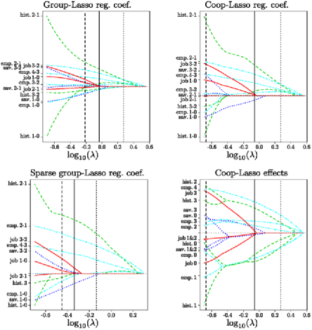
Figure 5: Regularization paths for four ordinal covariates (history, savings, job and employment) for the group, coop, and sparse group-Lasso on the contrast coefficients obtained from backward difference coding (top left, top right and bottom left, respectively). The transcription of contrasts to levels is also displayed for coop-Lasso (bottom right). The vertical lines mark the model selected by cross-validation on the validation set, for different criteria: deviance (plain), misclassification rate (dashed), and weighted misclassification error (dotted).

Recall that we only represent the ordinal covariates history, savings, employement and job. Each coefficient represents the increment between two adjacent levels, with positive and negative values resulting in an increase and decrease, respectively. Monotonicity with respect to all levels is reached if all the values corresponding to a factor are nonnegative or nonpositive. We also provide an alternative view of the coop-Lasso path, with the overall effects corresponding to levels, obtained by summing up the increments.

Most factors are not obviously amenable to quantitative coding since there is no natural distance between levels, but we, however, underline that using the usual quantitative transformation with equidistant values followed by linear regression would correspond here to identical increments between levels. Obviously, all displayed solutions radically contradict this linear trend hypothesis.

Our three solutions differ regarding monotonicity, which is almost never observed along the group-Lasso regularization path. The sparse group-Lasso paths have long sign-coherent sections, where group-Lasso infers slight wiggles. These sections extend further with the coop-Lasso. However, as the coop penalty goes to zero, sign-coherence is no longer preserved, and all methods eventually reach the same solution.

The sparse group and the coop-Lasso set some increments to zero, leading to the fusion of adjacent levels that should be welcomed regarding interpretation. The solutions tend to agree on these fusions on long sections of the paths, with some additional fusions of the sparse group-Lasso when slight monotonic solutions are provided by the coop-Lasso (see employment, levels 2 and 3, and savings levels 1 and 2). These fusions are perceived more directly on the coop-Lasso path of effects, displayed in the bottom right of Figure 5, where the effect of each level is displayed directly.

6.2 Robust microarray gene selection

Most studies on response to chemotherapy have considered breast cancer as a single homogeneous entity. However, it is a complex disease whose strong heterogeneity should not be overlooked. The data set proposed by Hess et al. (2006) consists in gene expression profiling of patients treated with chemotherapy prior to surgery, classified as presenting either a pathologic complete response (pCR) or a residual disease (not-pCR). It records the signal of 22,269 probes examining the human genome, each probe being related to a unique gene. Following Jeanmougin, Guedj and Ambroise (2011), we restrict our analysis to the basal tumors: for this particular subtype of breast cancer, clinical and pathologic features are homogeneous in the data set, whereas the response to chemotherapy is balanced, with 15 tumors being labeled pCR and 14 not-pCR. This setup is thus propitious to the statistical analysis of response to chemotherapy from the sole activity of genes.

6.2.1 Methodology

The usual processing of microarray data relies on probe measurements that are related to genes in the final interpretation of the statistical analysis. Here we would like to take a different stance, by gathering all the measurements associated to gene entities at an early stage of the statistical inference process. As a matter of fact, we typically observe that some probes related to the very same gene have different behaviors. Requiring a consensus at the gene level supports biological coherence, thus exercising caution in an inference process where statistically plausible explanations are numerous, due to the noisy probe signals and to the cumbersome $n\ll p$ setup (here $n=29$ and $p=22\mbox{,}269$). Since the probes related to a given gene relate to sequences that are predominantly cooperating, the sign-coherence assumed by the coop-Lasso is particularly appropriate to improve robustness to the measurement noise and to encourage biologically plausible solutions.

Our protocol includes a preselection of probes that facilitates the analysis for the nonadaptive penalization methods compared here, and also provides an assessment of the benefits of adding seemingly less relevant probes into the statistical analysis. We proceed as follows:

• select a restricted number $d$ of probes from classical differential analysis, where probes are sorted by increasing $p$-values;

• determine the genes associated to these $d$ probes, retrieve all the probes related to these genes, and select the corresponding $p$ probes, $p\geq d$, regardless of their signal;

• fit a model with group penalties where groups are defined by genes.

6.2.2 Experimental setup

We select the first $d=200$ most differentiated probes, as identified by the analysis of Jeanmougin, Guedj and Ambroise (2011), on the 22,269 probes for the $n=29$ patients with basal tumor. These 200 probes correspond to 172 genes, themselves associated to $p=381$ probes on the microarray as a whole, with 1 to 13 probes per gene. We clearly enter the high-dimensional setup with $p>13\times n$.

All signals are normalized to have a unitary within-class variance. We compare then the Lasso on the $d=200$ most differentiated probes, with the Lasso and group, sparse group and coop Lasso on the $p=381$ probes. All fits are produced with our code (available at http://stat.genopole.cnrs.fr/ logiciels/scoop).

Well-motivated analytical model selection criteria are not available today for Lasso-type penalties beyond the regression setup. Here, model selection is carried out by 5-fold cross-validation: we evaluate the $\mathrm{CV}$ error for each method with the same block partition using either the binomial deviance or the unweighted classification error.

6.2.3 Results

The 5-folds $\mathrm{CV}$ scores, either based on deviance or misclassification losses, are reported for each estimation method in Table 4, which also displays the number of selected groups and features for the models selected by minimizing the CV score.

Table 4: $\mathrm{CV}$ scores for misclassification error and binomial deviance on the basal tumor data. The minimizer of $\mathrm{CV}$ for misclassification and deviance are respectively denoted by $\lambda^{\mathrm{err}}$ and $\lambda^{\mathrm{dev}}$; the number of selected groups and features respectively refers to genes and probes

		Probes	Lasso	Group	Sparse	Coop
Model selection rule		CV score $\times 100$ (standard error)
Classification	$\lambda^{\mathrm{err}}$	10.3 (5.8)0	6.9 (4.9)	03.4 (3.5)	3.4 (3.5)	03.4 (3.5)
Deviance	$\lambda^{\mathrm{dev}}$	76.5 (37.6)	67.2 (32.3)	13.7 (8.1)	20.5 (10.0)	13.8 (7.9)
Model selection rule		# selected groups (features)
Classification	$\lambda^{\mathrm{err}}$	17 (17)	16 (17)	11 (15)	14 (21)	09 (11)
Deviance	$\lambda^{\mathrm{dev}}$	19 (19)	17 (18)	13 (21)	16 (26)	14 (18)

Expanding the set of probes from $d$ to $p$ slightly improves the performances of the Lasso, and considerable further progresses are brought by all group methods, which misclassify about 1 patient among the 29 and quarter deviance scores. As expected, less genes are selected by group methods; the difference is more important for the minimizers of the misclassification score, and, among those, for the group-Lasso and coop-Lasso that comply more stringently to the group structure. These observations indicate that the group structure defined by genes provides truly useful guidelines for inference.

The sparsity numbers differ among the group methods, coop-Lasso selecting as many genes as group-Lasso and fewer probes, and sparse group-Lasso retaining slightly more genes and probes. A more detailed picture is provided in Figure 6, which shows the regression coefficients for the three group estimators adjusted on the whole data set with their respective $\lambda^{\mathrm{err}}$ values.

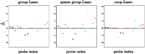
Figure 6: Logistic regression coefficients attached to each probe for group, sparse group and coop Lasso. Each marker (color and symbol) designates the gene associated to the probe: rnps1 (), msh6 (), prps2 (), h1fx (), mfge8 (), sulf1 (), rnf115 (), rnf38 (), thnsl2 () and edem3 ().

Among the three methods, a total of 15 groups (i.e., genes) are selected. For readability, we only represent the 10 leading groups of regression coefficients (according to their average norm). We first oberve that the magnitude of coefficients differs for each method, the coop-Lasso having the smallest one. In fact, there is a wide range of $\lambda^{\mathrm{err}}$ values for which the miclassification score is minimal for the coop-Lasso, enabling to choose a highly penalized solution without affecting accuracy. The magnitude apart, the group methods have qualitatively the same behaviors for all unitary groups but one, with thnsl2 () being set to zero by the coop-Lasso. The same patterns are observed for two other groups, rnps1 () and edem3 (), whose regression coefficients are consistently estimated to be sign-coherent. Then, sulf1 (), though being estimated sign-coherent by the sparse group-Lasso, is excluded from the support of the group and coop Lasso. Finally, msh6 (), estimated as sign incoherent with the two groups methods, is excluded from the support for the coop-Lasso.

Overall, the probe enrichment scheme we propose here leads to considerable improvements in prediction performance. This better statistical explanation is obtained without impairing interpretability, since sign-coherence is actually often satisfied by all methods and strictly enforced by the coop-Lasso. As often in this type of study, several methods provided similar prediction performances, but the explanation provided by the coop-Lasso is simpler, both from a statistical and from a biological viewpoint. Note that the coefficient paths (not shown) diverge early between the group and coop methods, so that the above-mentioned discrepancies are not simply due to model selection issues. As a final remark, we observed qualitatively similar behaviors when the initial number of probes $d$ ranged from 10 to 2000. For $d\leq 1000$, the group methods always performed best, with approximately identical classification errors, the group-Lasso and coop-Lasso slightly dominating the sparse group-Lasso in terms of deviance. With larger initial sets of probes, the enrichment procedure becomes less efficient, and all methods provide similar decaying results. The chosen setup displayed here, with $d=200$, leads to the smallest classification error for all methods, and was chosen for being representative of the most interesting regime.

7 Discussion

The coop-Lasso is a variant of the group-Lasso that was originally proposed in the context of multi-task learning, for inferring related networks with Gaussian Graphical Models [Chiquet, Grandvalet and Ambroise (2011)]. Here we develop its analysis in the linear regression setup and demonstrate its value for prediction and inference with generalized linear models. Along with this paper we provide an implementation of the fitting algorithm in the R package scoop, which makes this new penalized estimate publicly available for linear and logistic regression (the coop-Lasso for multiple network inference is also available in the R package simone).

The coop-Lasso differs from the group-Lasso and sparse group-Lasso [Friedman, Hastie and Tibshirani (2010)] by the assumption that the group structure is sign-coherent, namely, that groups gather either nonpositive, nonnegative or null parameters, enabling the recovery of various within-group sign patterns (positive, negative, null, nonpositive, nonnegative, nonnull). This flexibility greatly reduces the incentive to drive within-group sparsity with an additional parameter that later leads to an unwieldy model selection step. However, the relevance of the sign-coherence assumption should be firmly established since it plays an essential role in the performance of coop-Lasso compared to the sparse group-Lasso.

Under suitable irrepresentable conditions, the proposed penalty leads to consistent model selection, even when the true sparsity pattern does not match the group structure. When the groups are sign-coherent the coop-Lasso compares favorably to the group-Lasso, recovering the true support under the mildest assumptions.

We present an approximation of the effective degrees of freedom of the coop-Lasso which, once plugged into AIC or BIC, provides a fast way to select the tuning parameter in the linear regression setup. We provide empirical results demonstrating the capabilities of the coop-Lasso in terms of prediction and parameter selection, with BIC performing very well regarding support recovery even for small sample sizes.

We illustrate the merits of the coop-Lasso applied to the analysis to ordinal and continuous predictors. With an apposite coding, such as forward or backward difference coding, the sign-coherence assumption is transcribed in a monotonicity assumption, which does not require to stipulate the usual and controversial mapping from levels to quantitative variables. Finally, the application to genomic data opens a vast potential field of great practical interest for this type of penalty, both in terms of prediction and interpretability. Our forthcoming investigations will aim at substantiating this ambition by conducting large scale experiments in this application domain.

Appendix: Proofs

.1 Proof of Lemma 1

Let us use ${\cal T}_{k}$ as a shorthand for ${\cal S}_{k}(\bm{\beta})$, Chiquet, Grandvalet and Ambroise (2011) show that the subdifferential $\bm{\theta}$ obey the following conditions:

$$\displaystyle\max(\|\bm{\theta}_{\mathcal{G}_{k}}^{+}\|,\|\bm{\theta}_{\mathcal{G}_{k}}^{-}\|)\leq w_{k}\qquad\mbox{if }\bm{\beta}_{\mathcal{G}_{k}}=\mathbf{0},$$ (27a)

$$\displaystyle\bm{\theta}_{{\cal T}_{k}}=\frac{w_{k}\bm{\beta}_{{\cal T}_{k}}}{\|\bm{\beta}_{{\cal T}_{k}}\|},\qquad\|\bm{\theta}_{{\cal T}_{k}^{c}}^{-}\|\leq w_{k},\qquad\|\bm{\theta}_{{\cal T}_{k}^{c}}^{+}\|=0$$

$$\eqntext{\mbox{if }\|\bm{\beta}_{\mathcal{G}_{k}}^{+}\|>0,\|\bm{\beta}_{\mathcal{G}_{k}}^{-}\|=0,}$$ (27c)

$$\displaystyle\bm{\theta}_{{\cal T}_{k}}=\frac{w_{k}\bm{\beta}_{{\cal T}_{k}}}{\|\bm{\beta}_{{\cal T}_{k}}\|},\qquad\|\bm{\theta}_{{\cal T}_{k}^{c}}^{+}\|\leq w_{k},\qquad\|\bm{\theta}_{{\cal T}_{k}^{c}}^{-}\|=0$$

$$\eqntext{\mbox{if }\|\bm{\beta}_{\mathcal{G}_{k}}^{-}\|>0,\|\bm{\beta}_{\mathcal{G}_{k}}^{+}\|=0,}$$ (27e)

$$\displaystyle\forall j\in\mathcal{G}_{k}\qquad\bm{\theta}_{j}=w_{k}\bm{\beta}_{j}\|\operatorname{sign}(\beta_{j})\bm{\beta}\|^{-1}$$

$$\eqntext{\mbox{if }\|\bm{\beta}_{\mathcal{G}_{k}}^{-}\|>0,\|\bm{\beta}_{\mathcal{G}_{k}}^{+}\|>0.}$$ (27g)

We thus simply have to prove the equivalence of conditions (1) and (.1) for all $\bm{\beta}_{\mathcal{G}_{k}}$ values.

For $\bm{\beta}_{\mathcal{G}_{k}}=\mathbf{0}$, (1) reads

$$\|\bm{\theta}_{\mathcal{G}_{k}}^{+}\|\leq w_{k}\quad\mbox{and}\quad\|\bm{\theta}_{\mathcal{G}_{k}}^{-}\|\leq w_{k},$$ (28)

which is equivalent to (27a).

For $\bm{\beta}_{\mathcal{G}_{k}}\neq\mathbf{0}$, the equalities for $\bm{\theta}_{{\cal T}_{k}}$ in (.1)–(.1) are equivalent to (8a), thus setting the equivalence between (1) and (.1) for all nonzero coefficients. For $\bm{\beta}_{{\cal T}_{k}^{c}}$, let us consider the case (.1), where all nonzero parameters within group $k$ are positive. The first equation of (.1) implies that $\|\bm{\theta}_{{\cal T}_{k}}^{+}\|=w_{k}$ and $\|\bm{\theta}_{{\cal T}_{k}}^{-}\|=0$. Hence, $\|\bm{\theta}_{{\cal T}_{k}^{c}}^{-}\|\leq w_{k}$ and $\|\bm{\theta}_{{\cal T}_{k}^{c}}^{+}\|=0$ imply (28), so that (.1) implies (1). The contraposition is also easy to check. From (8a), when all coefficients are positive, we have that $\|\bm{\theta}_{{\cal T}_{k}}^{-}\|=0$ and $\|\bm{\theta}_{{\cal T}_{k}}^{+}\|=w_{k}$. Then, this implies that (8b) reads

$$\|\bm{\theta}_{{\cal T}_{k}^{c}}^{-}\|\leq w_{k}\quad\mbox{and}\quad\|\bm{\theta}_{{\cal T}_{k}^{c}}^{+}\|=0,$$

which defines $\bm{\theta}_{{\cal T}_{k}^{c}}$ in (.1). The proof is similar for (.1) where all nonzero parameters within group $k$ are positive.

.2 Proof of Proposition 1

We assume here that $\mathbf{X}^{\intercal}\mathbf{X}=\mathbf{I}_{p}$. We introduce the ridge estimator in the computation of the trace in equation (23), through the chain rule, yielding an unbiased estimate of $\operatorname{df}$:

$$\widetilde{\operatorname{df}}_{\mathrm{coop}}(\lambda) = \operatorname{tr}\biggl{(}\frac{\partial\hat{\mathbf{y}}(\lambda)}{\partial\mathbf{y}}\biggr{)}=\operatorname{tr}\biggl{(}\frac{\partial\mathbf{X}^{\intercal}\hat{\bm{\beta}}{}^{\mathrm{coop}}(\lambda)}{\partial\hat{\bm{\beta}}{}^{\mathrm{ridge}}(\gamma)}\,\frac{\partial\hat{\bm{\beta}}{}^{\mathrm{ridge}}(\gamma)}{\partial\mathbf{y}}\biggr{)}$$

$$= \frac{1}{1+\gamma}\sum_{k=1}^{K}\sum_{j\in\mathcal{G}_{k}}\frac{\partial\hat{\beta}{}^{\mathrm{coop}}_{j}(\lambda)}{\partial\hat{\beta}{}^{\mathrm{ridge}}_{j}(\gamma)},$$

where the last equation derives from the definition (25) of the ridge estimator with regularization parameter $\gamma$. Then, the expression of the coop-Lasso as a function of the ridge regression estimate is simply obtained from equation (11), using that, in the orthonormal case, we have $\hat{\bm{\beta}}{}^{\mathrm{ols}}=(1+\gamma)\hat{\bm{\beta}}{}^{\mathrm{ridge}}(\gamma)$. Dropping the reference to $\lambda$ and $\gamma$ that is obvious from the context, we have, $\forall k\in\{1,\ldots,K\}$ and $\forall j\in\mathcal{G}_{k}$,

$$\hat{\beta}_{j}^{\mathrm{coop}}=\biggl{(}1-\frac{\lambda w_{k}}{(1+\gamma)\|\bm{\varphi}_{j}(\hat{\bm{\beta}}{}^{\mathrm{ridge}}_{\mathcal{G}_{k}})\|}\biggr{)}^{+}(1+\gamma)\hat{\beta}_{j}^{\mathrm{ridge}}.$$ (29)

Then, for $j\in\mathcal{G}_{k}$, routine differentiation gives

$$\frac{1}{1+\gamma}\,\frac{\partial\hat{\beta}{}^{\mathrm{coop}}_{j}}{\partial\hat{\beta}{}^{\mathrm{ridge}}_{j}} = \mathbh{1}(\|\hat{\beta}{}^{\mathrm{coop}}_{j}\|>0)$$

$${}\times\biggl{(}1-\frac{\lambda w_{k}}{(1+\gamma)}\biggl{(}\frac{1}{\|\bm{\varphi}_{j}(\hat{\bm{\beta}}{}^{\mathrm{ridge}}_{\mathcal{G}_{k}})\|}-\frac{(\hat{\beta}{}^{\mathrm{ridge}}_{j})^{2}}{\|\bm{\varphi}_{j}(\hat{\bm{\beta}}{}^{\mathrm{ridge}}_{\mathcal{G}_{k}})\|^{3}}\biggr{)}\biggr{)}.$$

The summation over the positive and negative elements of $\mathcal{G}_{k}$ reduces to two terms

$$\frac{1}{1+\gamma}\sum_{j\in\mathcal{G}_{k}}\frac{\partial\hat{\beta}{}^{\mathrm{coop}}_{j}}{\partial\hat{\beta}{}^{\mathrm{ridge}}_{j}}$$

$$\qquad=\mathbh{1}\bigl{(}\|(\hat{\bm{\beta}}{}^{\mathrm{coop}}_{\mathcal{G}_{k}})^{+}\|>0\bigr{)}\biggl{(}p^{k}_{+}-\frac{\lambda w_{k}}{1+\gamma}\frac{(p^{k}_{+}-1)}{\|(\hat{\bm{\beta}}{}^{\mathrm{ridge}}_{\mathcal{G}_{k}})^{+}\|}\biggr{)}$$

$$\qquad\quad{}+\mathbh{1}\bigl{(}\|(\hat{\bm{\beta}}{}^{\mathrm{coop}}_{\mathcal{G}_{k}})^{-}\|>0\bigr{)}\biggl{(}p^{k}_{-}-\frac{\lambda w_{k}}{1+\gamma}\frac{(p^{k}_{-}-1)}{\|(\hat{\bm{\beta}}{}^{\mathrm{ridge}}_{\mathcal{G}_{k}})^{-}\|}\biggr{)}$$

$$\qquad=\mathbh{1}\bigl{(}\|(\hat{\bm{\beta}}{}^{\mathrm{coop}}_{\mathcal{G}_{k}})^{+}\|>0\bigr{)}+\biggl{(}1-\frac{\lambda w_{k}}{(1+\gamma)\|(\hat{\bm{\beta}}{}^{\mathrm{ridge}}_{\mathcal{G}_{k}})^{+}\|}\biggr{)}^{+}(p^{k}_{+}-1)$$

$$\qquad\quad{}+\mathbh{1}\bigl{(}\|(\hat{\bm{\beta}}{}^{\mathrm{coop}}_{\mathcal{G}_{k}})^{-}\|>0\bigr{)}+\biggl{(}1-\frac{\lambda w_{k}}{(1+\gamma)\|(\hat{\bm{\beta}}{}^{\mathrm{ridge}}_{\mathcal{G}_{k}})^{-}\|}\biggr{)}^{+}(p^{k}_{-}-1).$$

From (29), we have, $\forall k\in\{1,\ldots,K\}$ and $\forall j\in\mathcal{G}_{k},$

$$\biggl{(}1-\frac{\lambda w_{k}}{(1+\gamma)\|\bm{\varphi}_{j}(\hat{\bm{\beta}}{}^{\mathrm{ridge}}_{\mathcal{G}_{k}})\|}\biggr{)}^{+}=\frac{1}{1+\gamma}\frac{\|\bm{\varphi}_{j}(\hat{\bm{\beta}}{}^{\mathrm{coop}}_{\mathcal{G}_{k}})\|}{\|\bm{\varphi}_{j}(\hat{\bm{\beta}}{}^{\mathrm{ridge}}_{\mathcal{G}_{k}})\|},$$

which is used twice to simplify the previous expression. Summing over all groups concludes the proof.

.3 Proof of Theorem 2

Our asymptotic results are established on the scaled problem (19). We then follow the three steps proof technique proposed by Yuan and Lin (2007) for the Lasso and also applied by Bach (2008) for the group-Lasso: [(3)]

restrict the estimation problem to the true support;

complete this estimate by 0 outside the true support;

prove that this artificial estimate satisfies optimality conditions for the original coop-Lasso problem with probability tending to 1. Then, under (A2), the solution is unique, leading to the conclusion that the coop-Lasso estimator is equal to this artificial estimate with probability tending to 1, which ends the proof. Note, however, a slight yet important difference along the discussion: since we authorize divergences between the group structure $\{\mathcal{G}_{k}\}_{k=1}^{K}$ and the true support $\mathcal{S}$, the irrepresentable conditions (A4)–(A5) for the coop-Lasso cannot be expressed simply in terms of coop-norms [as it is done with the group-norm in Bach (2008)]. We will see that this does not impede the development of the proof.

As a first step, we prove two simple lemmas. Lemma 2 states that the coop-Lasso estimate, restricted on the true support $\mathcal{S}$, is consistent when $\lambda_{n}\to 0$. Lemma 3 provides the basis for the inequalities (17) and (18) that express our irrepresentable conditions.

Lemma 2

Assuming (A1)–(A3), let $\tilde{\bm{\beta}}{}_{\mathcal{S}}^{n}$ be the unique minimizer of the regression problem restricted to the true support $\mathcal{S}$:

$$\tilde{\bm{\beta}}{}_{\mathcal{S}}^{n}=\operatorname{\arg\min}\limits_{\mathbf{v}\in\mathbb{R}^{|\mathcal{S}|}}\frac{1}{2}\|\mathbf{y}-\mathbf{X}_{\centerdot\mathcal{S}}\mathbf{v}\|_{n}^{2}+\lambda_{n}\sum_{k\dvtx\mathcal{S}_{k}\neq\varnothing}w_{k}(\|\mathbf{v}_{\mathcal{S}_{k}}^{+}\|+\|\mathbf{v}_{\mathcal{S}_{k}}^{-}\|),$$

where $\|\cdot\|_{n}=\|\cdot\|/n$ denotes the empirical norm.

If $\lambda_{n}\rightarrow 0$, then $\tilde{\bm{\beta}}{}_{\mathcal{S}}^{n}\stackrel{{\scriptstyle P}}{{\longrightarrow}}\bm{\beta}^{\star}_{\mathcal{S}}.$

This lemma stems from standard results of M-estimation [van der Vaart (1998)]. Let $\bm{\varepsilon}=\mathbf{y}-\mathbf{X}\bm{\beta}^{\star}$, and write $\bm{\Psi}^{n}=\mathbf{X}^{\intercal}\mathbf{X}/n$. If $\lambda_{n}\rightarrow 0$, then under (A1)–(A2), for any $\mathbf{v}\in\mathbb{R}^{|\mathcal{S}|}$

$$Z_{n}(\mathbf{v}) = \frac{1}{2}\|\mathbf{y}-\mathbf{X}_{\centerdot\mathcal{S}}\mathbf{v}\|_{n}^{2}+\lambda_{n}\sum_{k\dvtx\mathcal{S}_{k}\neq\varnothing}w_{k}(\|\mathbf{v}_{\mathcal{S}_{k}}^{+}\|+\|\mathbf{v}_{\mathcal{S}_{k}}^{-}\|)$$

$$= \frac{1}{2}(\bm{\beta}^{\star}_{\mathcal{S}}-\mathbf{v})^{\intercal}\bm{\Psi}_{\mathcal{S}\mathcal{S}}^{n}(\bm{\beta}^{\star}_{\mathcal{S}}-\mathbf{v})-\frac{1}{n}\bm{\varepsilon}^{\intercal}\mathbf{X}_{\centerdot\mathcal{S}}(\bm{\beta}^{\star}_{\mathcal{S}}-\mathbf{v})+\frac{\bm{\varepsilon}^{\intercal}\bm{\varepsilon}}{2n}$$

$${}+\lambda_{n}\sum_{k,\mathcal{S}_{k}\neq\varnothing}w_{k}(\|\mathbf{v}_{\mathcal{S}_{k}}^{+}\|+\|\mathbf{v}_{\mathcal{S}_{k}}^{-}\|)$$

tends in probability to

$$Z(\mathbf{v})=\tfrac{1}{2}(\bm{\beta}^{\star}_{\mathcal{S}}-\mathbf{v})^{\intercal}\bm{\Psi}_{\mathcal{S}\mathcal{S}}(\bm{\beta}^{\star}_{\mathcal{S}}-\mathbf{v})+\tfrac{1}{2}\sigma^{2}.$$

It follows from the strict convexity of $Z_{n}$ that $\operatorname{\arg\min}\limits Z_{n}(\mathbf{v})\stackrel{{\scriptstyle P}}{{\longrightarrow}}\operatorname{\arg\min}\limits Z(\mathbf{v})=\bm{\beta}^{\star}_{\mathcal{S}}$ [Knight and Fu (2000)], which ends the proof.

Lemma 3

Consider a sequence of random variables $S_{n}$ such that $S_{n}\stackrel{{\scriptstyle P}}{{\longrightarrow}}S$. Suppose there exists $\delta>0$ such that for a given norm $\mu$ the limit $S$ is bounded away from 1:

$$\mu(S)\leq 1-\delta.$$

Then,

$$\mathbb{P}\bigl{(}\mu(S_{n})\leq 1\bigr{)}\rightarrow 1.$$

By triangular inequality and thanks to the constraint on $\mu(S)$,

$$\mathbb{P}\bigl{(}\mu(S_{n})\leq 1\bigr{)}\geq\mathbb{P}\bigl{(}\mu(S_{n}-S)\leq 1-\mu(S)\bigr{)}\geq\mathbb{P}\bigl{(}\mu(S_{n}-S)\leq\delta\bigr{)},$$

Convergence in probability of $S_{n}$ to $S$ concludes the proof:

$$\mathbb{P}\bigl{(}\mu(S_{n}-S)\leq\delta\bigr{)}\rightarrow 1\qquad\mbox{therefore }\mathbb{P}\bigl{(}\mu(S_{n})\leq 1\bigr{)}\rightarrow 1.$$

Let us consider the full vector $\tilde{\bm{\beta}}{}^{n}$ with coefficients $\tilde{\bm{\beta}}{}_{\mathcal{S}}^{n}$ defined as in Lemma 2 and other coefficients null, $\tilde{\bm{\beta}}{}_{\mathcal{S}^{c}}^{n}=\mathbf{0}$. We now proceed to the last step of the proof of Theorem 2, by proving that $\tilde{\bm{\beta}}{}^{n}$ satisfies the coop-Lasso optimality conditions with probability tending to 1 under the additional conditions (A4)–(A5). The final conclusion then results from the uniqueness of the coop-Lasso estimator.

First, consider optimality conditions with respect to $\bm{\beta}_{\mathcal{S}}$. As a result of Lemma 2, the probability that $\tilde{\bm{\beta}}{}_{j}^{n}\neq 0$ for every $j\in\mathcal{S}$ tends to 1. Thereby, $\tilde{\bm{\beta}}{}_{\mathcal{S}}^{n}$ satisfies (9a) on the restriction of $\mathbf{X}$ to covariates in $\mathcal{S}$ with probability tending to 1. As $\tilde{\bm{\beta}}{}_{\mathcal{S}^{c}}^{n}=\mathbf{0}$, then $\mathbf{X}\tilde{\bm{\beta}}{}^{n}=\mathbf{X}_{\centerdot\mathcal{S}}\tilde{\bm{\beta}}{}_{\mathcal{S}}^{n}$ and for every $j\in\mathcal{S}$, $\|\bm{\varphi}_{j}(\tilde{\bm{\beta}}{}_{\mathcal{S}_{k}})^{n}\|=\|\bm{\varphi}_{j}(\tilde{\bm{\beta}}{}_{\mathcal{G}_{k}}^{n})\|$, therefore, $\tilde{\bm{\beta}}{}_{\mathcal{S}}^{n}$ satisfies (9a) in the original problem with probability tending to 1.

Second, $\tilde{\bm{\beta}}{}_{\mathcal{S}^{c}}^{n}$ should also verify the optimality conditions (1) with probability tending to 1. With assumption (A3), we only have to consider two cases that read:

• if group $k$ is excluded from the support, one must have

  $$\mathbb{P}\bigl{(}\max\bigl{(}\bigl{\|}\bigl{(}(\mathbf{X}_{\centerdot\mathcal{S}_{k}^{c}})^{\intercal}(\mathbf{X}\tilde{\bm{\beta}}{}^{n}-\mathbf{y})\bigr{)}^{+}\bigr{\|}_{n},\bigl{\|}\bigl{(}(\mathbf{X}_{\centerdot\mathcal{S}_{k}^{c}})^{\intercal}(\mathbf{X}\tilde{\bm{\beta}}{}^{n}-\mathbf{y})\bigr{)}^{-}\bigr{\|}_{n}\bigr{)}\leq\lambda_{n}w_{k}\bigr{)}$$

  (30)

  $$\qquad\rightarrow 1;$$

• if group $k$ intersects the support, with either positive ($\nu_{k}=1$) or negative ($\nu_{k}=-1$) coefficients, one must have

  $$\mathbb{P}\bigl{(}\{\nu_{k}(\mathbf{X}_{\centerdot\mathcal{S}_{k}^{c}})^{\intercal}(\mathbf{X}\tilde{\bm{\beta}}{}^{n}-\mathbf{y})\succeq\mathbf{0}\}\cap\{\|(\mathbf{X}_{\centerdot\mathcal{S}_{k}^{c}})^{\intercal}(\mathbf{X}\tilde{\bm{\beta}}{}^{n}-\mathbf{y})\|_{n}\leq\lambda_{n}w_{k}\}\bigr{)}\rightarrow 1.$$ (31)

To prove (• ‣ .3) and (31), we study the asymptotics of $(\mathbf{X}_{\centerdot\mathcal{S}_{k}^{c}})^{\intercal}(\mathbf{X}\tilde{\bm{\beta}}{}^{n}-\mathbf{y})/n$ for any group such that $\mathcal{S}_{k}^{c}$ is not empty. As a consequence of the existence of the fourth order moments of the centered random variables $X$ and $Y$, the multivariate central limit theorem applies, yielding

$$\frac{\mathbf{X}^{\intercal}\mathbf{X}}{n} = \frac{1}{n}\sum_{i=1}^{n}\mathbf{x}_{i}^{\intercal}\mathbf{x}_{i}=\bm{\Psi}+O_{P}(n^{-1/2}),$$

$$\frac{\mathbf{X}^{\intercal}\bm{\varepsilon}}{n} = \frac{1}{n}\sum_{i=1}^{n}\mathbf{x}_{i}\bm{\varepsilon}_{i}=O_{P}(n^{-1/2})$$

Then, we derive from (.3) and the definition of $\tilde{\bm{\beta}}{}^{n}$ that

$$\frac{1}{n}(\mathbf{X}_{\centerdot\mathcal{S}_{k}^{c}})^{\intercal}(\mathbf{X}\tilde{\bm{\beta}}{}^{n}-\mathbf{y}) = \frac{1}{n}(\mathbf{X}_{\centerdot\mathcal{S}_{k}^{c}})^{\intercal}\mathbf{X}(\tilde{\bm{\beta}}{}^{n}-\bm{\beta}^{\star})-\frac{1}{n}(\mathbf{X}_{\centerdot\mathcal{S}_{k}^{c}})^{\intercal}\bm{\varepsilon}$$

$$= \frac{1}{n}(\mathbf{X}_{\centerdot\mathcal{S}_{k}^{c}})^{\intercal}\mathbf{X}_{\centerdot\mathcal{S}}(\tilde{\bm{\beta}}{}_{\mathcal{S}}^{n}-\bm{\beta}_{\mathcal{S}}^{\star})+O_{P}(n^{-1/2})$$

$$= \bm{\Psi}_{\mathcal{S}_{k}^{c}\mathcal{S}}(\tilde{\bm{\beta}}{}_{\mathcal{S}}^{n}-\bm{\beta}_{\mathcal{S}}^{\star})+O_{P}(n^{-1/2}),$$

while the combination of (.3) and optimality conditions (9a) on $\tilde{\bm{\beta}}{}_{\mathcal{S}}^{n}$ leads to

$$\bm{\Psi}_{\mathcal{S}\mathcal{S}}(\tilde{\bm{\beta}}{}_{\mathcal{S}}^{n}-\bm{\beta}_{\mathcal{S}}^{\star})=-\lambda_{n}\mathbf{D}(\tilde{\bm{\beta}}{}_{\mathcal{S}}^{n})\tilde{\bm{\beta}}{}_{\mathcal{S}}^{n}+O_{P}(n^{-1/2}),$$ (33)

where $\mathbf{D}(\cdot)$ is the weighting matrix (16). Put (.3) and (33) together to finally obtain

$$\frac{1}{n}(\mathbf{X}_{\centerdot\mathcal{S}_{k}^{c}})^{\intercal}(\mathbf{X}\tilde{\bm{\beta}}{}^{n}-\mathbf{y})=-\lambda_{n}\bm{\Psi}_{\mathcal{S}_{k}^{c}\mathcal{S}}\bm{\Psi}_{\mathcal{S}\mathcal{S}}^{-1}\mathbf{D}(\tilde{\bm{\beta}}{}_{\mathcal{S}}^{n})\tilde{\bm{\beta}}{}_{\mathcal{S}}^{n}+O_{P}(n^{-1/2}).$$ (34)

Now, define for any $k$ such that $\mathcal{S}_{k}^{c}$ is not empty:

$$R_{k,n}=\frac{1}{w_{k}\lambda_{n}}\frac{1}{n}(\mathbf{X}_{\centerdot\mathcal{S}_{k}^{c}})^{\intercal}(\mathbf{X}\tilde{\bm{\beta}}{}^{n}-\mathbf{y})\quad\mbox{and}\quad R_{k}=-\frac{1}{w_{k}}\bm{\Psi}_{\mathcal{S}_{k}^{c}\mathcal{S}}\bm{\Psi}_{\mathcal{S}\mathcal{S}}^{-1}\mathbf{D}(\bm{\beta}^{\star}_{\mathcal{S}})\bm{\beta}^{\star}_{\mathcal{S}}.$$

Limits (• ‣ .3) and (31) are expressed:

• if group $k$ is excluded from the support, one must have

  $$\mathbb{P}\bigl{(}\max(\|R_{k,n}^{+}\|,\|R_{k,n}^{-}\|)\leq 1\bigr{)}\rightarrow 1;$$

• if group $k$ intersects the support, with either positive ($\nu_{k}=1$) or negative ($\nu_{k}=-1$) coefficients, one must have

  $$\mathbb{P}\bigl{(}\{\nu_{k}R_{k,n}\succeq\mathbf{0}\}\cap\{\|(\nu_{k}R_{k,n})^{+}\|\leq 1\}\bigr{)}\rightarrow 1.$$

Remark that, as a continuous function of $\tilde{\bm{\beta}}{}_{\mathcal{S}}^{n}$, $\mathbf{D}(\tilde{\bm{\beta}}{}_{\mathcal{S}}^{n})\tilde{\bm{\beta}}{}_{\mathcal{S}}^{n}$ converges in probability to $\mathbf{D}(\bm{\beta}^{\star}_{\mathcal{S}})\bm{\beta}^{\star}_{\mathcal{S}}$. Therefore, with a decrease rate for $\lambda_{n}$ chosen such that $n^{1/2}\lambda_{n}\rightarrow\infty$, equation (34) implies

$$R_{k,n}\stackrel{{\scriptstyle P}}{{\longrightarrow}}R_{k}.$$ (35)

It now suffices to successively apply Lemma 3 to the appropriate vectors and norms to show that $\tilde{\bm{\beta}}{}_{\mathcal{S}^{c}}^{n}$ satisfies (• ‣ .3) and (31):

• if group $k$ is excluded from the support, (A4) assumes that there exists $\eta>0$, such that

  $$\max(\|R_{k}^{+}\|,\|R_{k}^{-}\|)\leq 1-\eta,$$

  and Lemma 3 applied to $\mu(u)=\max(\|u^{+}\|,\|u^{-}\|)$ provides

  $$\mathbb{P}\{\max(\|R_{k,n}^{+}\|,\|R_{k,n}^{-}\|)\leq 1\}\rightarrow 1.$$

• if group $k$ intersects the support, with either positive ($\nu_{k}=1$) or negative ($\nu_{k}=-1$) coefficients,

  $$\mathbb{P}\bigl{(}\{\|(\nu_{k}R_{k,n})^{+}\|\leq 1\}\cap\{\nu_{k}R_{k,n}\succeq\mathbf{0}\}\bigr{)}$$

  $$\qquad=1-\mathbb{P}\bigl{(}\{\|(\nu_{k}R_{k,n})^{+}\|>1\}\cup\{\nu_{k}R_{k,n}\prec\mathbf{0}\}\bigr{)}$$

  $$\qquad\geq 1-\mathbb{P}\bigl{(}\|(\nu_{k}R_{k,n})^{+}\|>1\bigr{)}-\mathbb{P}(\nu_{k}R_{k,n}\prec\mathbf{0})$$

  $$\qquad\geq 1-\mathbb{P}\bigl{(}\max(\|R_{k,n}^{+}\|,\|R_{k,n}^{-}\|)>1\bigr{)}-\mathbb{P}(\nu_{k}R_{k,n}\prec\mathbf{0}).$$

  As previously, the first probability in the sum tends to 0 because of (A4) and Lemma 3. The second probability tends to 0 from (A5) and of the convergence in probability of $R_{k,n}$ to $R_{k}$. Therefore, the overall probability tends to 1.

Denote by $A_{k,n}$ these events on which coefficients in $\mathcal{S}_{k}^{c}$ are set to 0. We just showed that individually for each group $k$ with true null coefficients, $P(A_{k,n})\rightarrow 1$. This implies that

$$\mathbb{P}\biggl{(}\bigcup_{k\dvtx\mathcal{S}_{k}^{c}\neq\varnothing}A^{c}_{k,n}\biggr{)}\leq\sum_{k\dvtx\mathcal{S}_{k}^{c}\neq\varnothing}\mathbb{P}(A_{k,n}^{c})\rightarrow 0,$$

which in turn concludes the proof:

$$\mathbb{P}\biggl{(}\bigcap_{k\dvtx\mathcal{S}_{k}^{c}\neq\varnothing}A_{k,n}\biggr{)}\rightarrow 1.$$

References

- Bach (2008) {barticle}[mr] \bauthor\bsnmBach, \bfnmFrancis R.\binitsF. R. (\byear2008). \btitleConsistency of the group lasso and multiple kernel learning. \bjournalJ. Mach. Learn. Res. \bvolume9 \bpages1179–1225. \bidissn=1532-4435, mr=2417268 \bptokimsref \endbibitem
- Bakin (1999) {bphdthesis}[author] \bauthor\bsnmBakin, \bfnmS.\binitsS. (\byear1999). \btitleAdaptive regression and model selection in data mining problems. \btypePh.D. thesis, \bschoolAustralian National Univ., Canberra. \bptokimsref \endbibitem
- Beck and Teboulle (2009) {barticle}[mr] \bauthor\bsnmBeck, \bfnmAmir\binitsA. and \bauthor\bsnmTeboulle, \bfnmMarc\binitsM. (\byear2009). \btitleA fast iterative shrinkage-thresholding algorithm for linear inverse problems. \bjournalSIAM J. Imaging Sci. \bvolume2 \bpages183–202. \bidissn=1936-4954, mr=2486527 \bptokimsref \endbibitem
- Breiman (1995) {barticle}[mr] \bauthor\bsnmBreiman, \bfnmLeo\binitsL. (\byear1995). \btitleBetter subset regression using the nonnegative garrote. \bjournalTechnometrics \bvolume37 \bpages373–384. \bidissn=0040-1706, mr=1365720 \bptokimsref \endbibitem
- Breiman (1996) {barticle}[mr] \bauthor\bsnmBreiman, \bfnmLeo\binitsL. (\byear1996). \btitleHeuristics of instability and stabilization in model selection. \bjournalAnn. Statist. \bvolume24 \bpages2350–2383. \biddoi=10.1214/aos/1032181158, issn=0090-5364, mr=1425957 \bptokimsref \endbibitem
- Breiman et al. (1984) {bbook}[author] \bauthor\bsnmBreiman, \bfnmL.\binitsL., \bauthor\bsnmFriedman, \bfnmJ. H.\binitsJ. H., \bauthor\bsnmOlshen, \bfnmR.\binitsR. and \bauthor\bsnmStone, \bfnmC. J.\binitsC. J. (\byear1984). \btitleClassification and Regression Trees. \bpublisherWadsworth, \baddressBelmont, CA. \bptokimsref \endbibitem
- Chiquet, Grandvalet and Ambroise (2011) {barticle}[author] \bauthor\bsnmChiquet, \bfnmJ.\binitsJ., \bauthor\bsnmGrandvalet, \bfnmY\binitsY. and \bauthor\bsnmAmbroise, \bfnmC.\binitsC. (\byear2011). \btitleInferring multiple graphical structures. \bjournalStatistic and Computing \bvolume21 \bpages537–553. \bptokimsref \endbibitem
- Efron (2004) {barticle}[mr] \bauthor\bsnmEfron, \bfnmBradley\binitsB. (\byear2004). \btitleThe estimation of prediction error: Covariance penalties and cross-validation. \bjournalJ. Amer. Statist. Assoc. \bvolume99 \bpages619–642. \biddoi=10.1198/016214504000000692, issn=0162-1459, mr=2090899 \bptnotecheck related\bptokimsref \endbibitem
- Eisen et al. (1998) {barticle}[pbm] \bauthor\bsnmEisen, \bfnmM. B.\binitsM. B., \bauthor\bsnmSpellman, \bfnmP. T.\binitsP. T., \bauthor\bsnmBrown, \bfnmP. O.\binitsP. O. and \bauthor\bsnmBotstein, \bfnmD.\binitsD. (\byear1998). \btitleCluster analysis and display of genome-wide expression patterns. \bjournalProc. Natl. Acad. Sci. USA \bvolume95 \bpages14863–14868. \bidissn=0027-8424, pmcid=24541, pmid=9843981 \bptokimsref \endbibitem
- Foygel and Drton (2010) {bmisc}[author] \bauthor\bsnmFoygel, \bfnmR.\binitsR. and \bauthor\bsnmDrton, \bfnmM.\binitsM. (\byear2010). \bhowpublishedExact block-wise optimization in group lasso for linear regression. Technical report. Available at arXiv:\arxivurl1010.3320. \bptokimsref \endbibitem
- Frank and Asuncion (2010) {bmisc}[author] \bauthor\bsnmFrank, \bfnmA.\binitsA. and \bauthor\bsnmAsuncion, \bfnmA.\binitsA. (\byear2010). \btitleUCI machine learning repository. \bptokimsref \endbibitem
- Friedman, Hastie and Tibshirani (2010) {bmisc}[author] \bauthor\bsnmFriedman, \bfnmJ.\binitsJ., \bauthor\bsnmHastie, \bfnmT.\binitsT. and \bauthor\bsnmTibshirani, \bfnmR.\binitsR. (\byear2010). \bhowpublishedA note on the group Lasso and a sparse group Lasso. Technical report. Available at arXiv:\arxivurl1001.0736. \bptokimsref \endbibitem
- Gertheiss and Tutz (2009) {barticle}[author] \bauthor\bsnmGertheiss, \bfnmJ.\binitsJ. and \bauthor\bsnmTutz, \bfnmG.\binitsG. (\byear2009). \btitlePenalized regression with ordinal predictors. \bjournalInternational Statistical Review \bvolume77 \bpages345–365. \bptokimsref \endbibitem
- Gertheiss and Tutz (2010) {barticle}[mr] \bauthor\bsnmGertheiss, \bfnmJan\binitsJ. and \bauthor\bsnmTutz, \bfnmGerhard\binitsG. (\byear2010). \btitleSparse modeling of categorial explanatory variables. \bjournalAnn. Appl. Stat. \bvolume4 \bpages2150–2180. \biddoi=10.1214/10-AOAS355, issn=1932-6157, mr=2829951 \bptokimsref \endbibitem
- Grandvalet and Canu (1999) {binproceedings}[author] \bauthor\bsnmGrandvalet, \bfnmY.\binitsY. and \bauthor\bsnmCanu, \bfnmS.\binitsS. (\byear1999). \btitleOutcomes of the equivalence of adaptive ridge with least absolute shrinkage. In \bbooktitleAdvances in Neural Information Processing Systems 11 (NIPS 1998) \bpages445–451. \bptokimsref \endbibitem
- Hess et al. (2006) {barticle}[author] \bauthor\bsnmHess, \bfnmK. R.\binitsK. R., \bauthor\bsnmAnderson, \bfnmK.\binitsK., \bauthor\bsnmSymmans, \bfnmW. F.\binitsW. F., \bauthor\bsnmValero, \bfnmV.\binitsV., \bauthor\bsnmIbrahim, \bfnmN.\binitsN., \bauthor\bsnmMejia, \bfnmJ. A.\binitsJ. A., \bauthor\bsnmBooser, \bfnmD.\binitsD., \bauthor\bsnmTheriault, \bfnmR. L.\binitsR. L., \bauthor\bsnmBuzdar, \bfnmU.\binitsU., \bauthor\bsnmDempsey, \bfnmP. J.\binitsP. J., \bauthor\bsnmRouzier, \bfnmR.\binitsR., \bauthor\bsnmSneige, \bfnmN.\binitsN., \bauthor\bsnmRoss, \bfnmJ. S.\binitsJ. S., \bauthor\bsnmVidaurre, \bfnmT.\binitsT., \bauthor\bsnmGómez, \bfnmH. L.\binitsH. L., \bauthor\bsnmHortobagyi, \bfnmG. N.\binitsG. N. and \bauthor\bsnmPustzai, \bfnmL.\binitsL. (\byear2006). \btitlePharmacogenomic predictor of sensitivity to preoperative chemotherapy with Paclitaxel and Fluorouracil, Doxorubicin, and Cyclophosphamide in breast cancer. \bjournalJournal of Clinical Oncology \bvolume24 \bpages4236–4244. \bptokimsref \endbibitem
- Hesterberg et al. (2008) {barticle}[mr] \bauthor\bsnmHesterberg, \bfnmTim\binitsT., \bauthor\bsnmChoi, \bfnmNam Hee\binitsN. H., \bauthor\bsnmMeier, \bfnmLukas\binitsL. and \bauthor\bsnmFraley, \bfnmChris\binitsC. (\byear2008). \btitleLeast angle and penalized regression: A review. \bjournalStat. Surv. \bvolume2 \bpages61–93. \biddoi=10.1214/08-SS035, issn=1935-7516, mr=2520981 \bptokimsref \endbibitem
- Huang and Zhang (2010) {barticle}[mr] \bauthor\bsnmHuang, \bfnmJunzhou\binitsJ. and \bauthor\bsnmZhang, \bfnmTong\binitsT. (\byear2010). \btitleThe benefit of group sparsity. \bjournalAnn. Statist. \bvolume38 \bpages1978–2004. \biddoi=10.1214/09-AOS778, issn=0090-5364, mr=2676881 \bptokimsref \endbibitem
- Jeanmougin, Guedj and Ambroise (2011) {barticle}[author] \bauthor\bsnmJeanmougin, \bfnmM.\binitsM., \bauthor\bsnmGuedj, \bfnmM.\binitsM. and \bauthor\bsnmAmbroise, \bfnmC.\binitsC. (\byear2011). \btitleDefining a robust biological prior from pathway analysis to drive network inference. \bjournalJ. SFdS \bvolume152 \bpages97–110. \bidmr=2821224 \bptokimsref \endbibitem
- Knight and Fu (2000) {barticle}[mr] \bauthor\bsnmKnight, \bfnmKeith\binitsK. and \bauthor\bsnmFu, \bfnmWenjiang\binitsW. (\byear2000). \btitleAsymptotics for lasso-type estimators. \bjournalAnn. Statist. \bvolume28 \bpages1356–1378. \biddoi=10.1214/aos/1015957397, issn=0090-5364, mr=1805787 \bptokimsref \endbibitem
- Ma, Song and Huang (2007) {barticle}[pbm] \bauthor\bsnmMa, \bfnmShuangge\binitsS., \bauthor\bsnmSong, \bfnmXiao\binitsX. and \bauthor\bsnmHuang, \bfnmJian\binitsJ. (\byear2007). \btitleSupervised group Lasso with applications to microarray data analysis. \bjournalBMC Bioinformatics \bvolume8 \bpages60. \biddoi=10.1186/1471-2105-8-60, issn=1471-2105, pii=1471-2105-8-60, pmcid=1821041, pmid=17316436 \bptokimsref \endbibitem
- Meier, van de Geer and Bühlmann (2008) {barticle}[mr] \bauthor\bsnmMeier, \bfnmLukas\binitsL., \bauthor\bparticlevan de \bsnmGeer, \bfnmSara\binitsS. and \bauthor\bsnmBühlmann, \bfnmPeter\binitsP. (\byear2008). \btitleThe group Lasso for logistic regression. \bjournalJ. R. Stat. Soc. Ser. B Stat. Methodol. \bvolume70 \bpages53–71. \biddoi=10.1111/j.1467-9868.2007.00627.x, issn=1369-7412, mr=2412631 \bptokimsref \endbibitem
- Nardi and Rinaldo (2008) {barticle}[mr] \bauthor\bsnmNardi, \bfnmYuval\binitsY. and \bauthor\bsnmRinaldo, \bfnmAlessandro\binitsA. (\byear2008). \btitleOn the asymptotic properties of the group lasso estimator for linear models. \bjournalElectron. J. Stat. \bvolume2 \bpages605–633. \biddoi=10.1214/08-EJS200, issn=1935-7524, mr=2426104 \bptokimsref \endbibitem
- Osborne, Presnell and Turlach (2000) {barticle}[mr] \bauthor\bsnmOsborne, \bfnmMichael R.\binitsM. R., \bauthor\bsnmPresnell, \bfnmBrett\binitsB. and \bauthor\bsnmTurlach, \bfnmBerwin A.\binitsB. A. (\byear2000). \btitleOn the LASSO and its dual. \bjournalJ. Comput. Graph. Statist. \bvolume9 \bpages319–337. \biddoi=10.2307/1390657, issn=1061-8600, mr=1822089 \bptokimsref \endbibitem
- Park, Hastie and Tibshirani (2007) {barticle}[pbm] \bauthor\bsnmPark, \bfnmMee Young\binitsM. Y., \bauthor\bsnmHastie, \bfnmTrevor\binitsT. and \bauthor\bsnmTibshirani, \bfnmRobert\binitsR. (\byear2007). \btitleAveraged gene expressions for regression. \bjournalBiostatistics \bvolume8 \bpages212–227. \biddoi=10.1093/biostatistics/kxl002, issn=1465-4644, pii=kxl002, pmid=16698769 \bptnotecheck year\bptokimsref \endbibitem
- Roth and Fischer (2008) {binproceedings}[author] \bauthor\bsnmRoth, \bfnmV.\binitsV. and \bauthor\bsnmFischer, \bfnmB.\binitsB. (\byear2008). \btitleThe group-Lasso for generalized linear models: Uniqueness of solutions and efficient algorithms. In \bbooktitleICML’08: Proceedings of the 25th International Conference on Machine Learning \bpages848–855. \bptokimsref \endbibitem
- Rufibach (2010) {barticle}[mr] \bauthor\bsnmRufibach, \bfnmKaspar\binitsK. (\byear2010). \btitleAn active set algorithm to estimate parameters in generalized linear models with ordered predictors. \bjournalComput. Statist. Data Anal. \bvolume54 \bpages1442–1456. \biddoi=10.1016/j.csda.2010.01.014, issn=0167-9473, mr=2600846 \bptokimsref \endbibitem
- Serlin and Levin (1985) {barticle}[author] \bauthor\bsnmSerlin, \bfnmR. C.\binitsR. C. and \bauthor\bsnmLevin, \bfnmJ. R.\binitsJ. R. (\byear1985). \btitleTeaching how to derive directly interpretable coding schemes for multiple regression analysis. \bjournalJournal of Educational Statistics \bvolume10 \bpages223–238. \bptokimsref \endbibitem
- Stein (1981) {barticle}[mr] \bauthor\bsnmStein, \bfnmCharles M.\binitsC. M. (\byear1981). \btitleEstimation of the mean of a multivariate normal distribution. \bjournalAnn. Statist. \bvolume9 \bpages1135–1151. \bidissn=0090-5364, mr=0630098 \bptokimsref \endbibitem
- Tibshirani (1996) {barticle}[mr] \bauthor\bsnmTibshirani, \bfnmRobert\binitsR. (\byear1996). \btitleRegression shrinkage and selection via the lasso. \bjournalJ. Roy. Statist. Soc. Ser. B \bvolume58 \bpages267–288. \bidissn=0035-9246, mr=1379242 \bptokimsref \endbibitem
- van der Vaart (1998) {bbook}[mr] \bauthor\bparticlevan der \bsnmVaart, \bfnmA. W.\binitsA. W. (\byear1998). \btitleAsymptotic Statistics. \bseriesCambridge Series in Statistical and Probabilistic Mathematics \bvolume3. \bpublisherCambridge Univ. Press, \baddressCambridge. \bidmr=1652247 \bptokimsref \endbibitem
- Yuan and Lin (2006) {barticle}[mr] \bauthor\bsnmYuan, \bfnmMing\binitsM. and \bauthor\bsnmLin, \bfnmYi\binitsY. (\byear2006). \btitleModel selection and estimation in regression with grouped variables. \bjournalJ. R. Stat. Soc. Ser. B Stat. Methodol. \bvolume68 \bpages49–67. \biddoi=10.1111/j.1467-9868.2005.00532.x, issn=1369-7412, mr=2212574 \bptokimsref \endbibitem
- Yuan and Lin (2007) {barticle}[mr] \bauthor\bsnmYuan, \bfnmMing\binitsM. and \bauthor\bsnmLin, \bfnmYi\binitsY. (\byear2007). \btitleOn the non-negative garrote estimator. \bjournalJ. R. Stat. Soc. Ser. B Stat. Methodol. \bvolume69 \bpages143–161. \biddoi=10.1111/j.1467-9868.2007.00581.x, issn=1369-7412, mr=2325269 \bptokimsref \endbibitem
- Zhao, Rocha and Yu (2009) {barticle}[mr] \bauthor\bsnmZhao, \bfnmPeng\binitsP., \bauthor\bsnmRocha, \bfnmGuilherme\binitsG. and \bauthor\bsnmYu, \bfnmBin\binitsB. (\byear2009). \btitleThe composite absolute penalties family for grouped and hierarchical variable selection. \bjournalAnn. Statist. \bvolume37 \bpages3468–3497. \biddoi=10.1214/07-AOS584, issn=0090-5364, mr=2549566 \bptokimsref \endbibitem
- Zhou et al. (2010) {barticle}[pbm] \bauthor\bsnmZhou, \bfnmHua\binitsH., \bauthor\bsnmSehl, \bfnmMary E.\binitsM. E., \bauthor\bsnmSinsheimer, \bfnmJanet S.\binitsJ. S. and \bauthor\bsnmLange, \bfnmKenneth\binitsK. (\byear2010). \btitleAssociation screening of common and rare genetic variants by penalized regression. \bjournalBioinformatics \bvolume26 \bpages2375–2382. \biddoi=10.1093/bioinformatics/btq448, issn=1367-4811, pii=btq448, pmcid=3025646, pmid=20693321 \bptokimsref \endbibitem
- Zou and Hastie (2005) {barticle}[mr] \bauthor\bsnmZou, \bfnmHui\binitsH. and \bauthor\bsnmHastie, \bfnmTrevor\binitsT. (\byear2005). \btitleRegularization and variable selection via the elastic net. \bjournalJ. R. Stat. Soc. Ser. B Stat. Methodol. \bvolume67 \bpages301–320. \biddoi=10.1111/j.1467-9868.2005.00503.x, issn=1369-7412, mr=2137327 \bptokimsref \endbibitem
- Zou, Hastie and Tibshirani (2007) {barticle}[mr] \bauthor\bsnmZou, \bfnmHui\binitsH., \bauthor\bsnmHastie, \bfnmTrevor\binitsT. and \bauthor\bsnmTibshirani, \bfnmRobert\binitsR. (\byear2007). \btitleOn the “degrees of freedom” of the lasso. \bjournalAnn. Statist. \bvolume35 \bpages2173–2192. \biddoi=10.1214/009053607000000127, issn=0090-5364, mr=2363967 \bptokimsref \endbibitem