Disentangling star formation and merger growth in the evolution of Luminous Red Galaxies

Abstract

We introduce a novel technique for empirically understanding galaxy evolution. We use empirically determined stellar evolution models to predict the past evolution of the Sloan Digital Sky Survey (SDSS-II) Luminous Red Galaxy (LRG) sample without any a-priori assumption about galaxy evolution. By carefully contrasting the evolution of the predicted and observed number and luminosity densities we test the passive evolution scenario for galaxies of different luminosity, and determine minimum merger rates. We find that the LRG population is not purely coeval, with some of galaxies targeted at $z<0.23$ and at $z>0.34$ showing different dynamical growth than galaxies targeted throughout the sample. Our results show that the LRG population is dynamically growing, and that this growth must be dominated by the faint end. For the most luminous galaxies, we find lower minimum merger rates than required by previous studies that assume passive stellar evolution, suggesting that some of the dynamical evolution measured previously was actually due to galaxies with non-passive stellar evolution being incorrectly modelled. Our methodology can be used to identify and match coeval populations of galaxies across cosmic times, over one or more surveys.

1 Introduction

The most recent observational evidence points towards a model of structure and galaxy formation that is hierarchical in nature: small fluctuations in the matter density field grow via gravity, with their dynamics being governed in detail by dark matter and dark energy. Baryons trace the dark matter and, in regions of sufficient gravitational depth, they accumulate and form stars and galaxies (White & Rees, 1978). As the matter field continues to evolve dynamically - largely oblivious to this process - the stellar content of galaxies grows via a combination of two modes: forming new stars from cold gas, and merging with other galaxies.

LRGs are extensively used as cosmological probes (e.g. Reid et al. 2010; Percival et al. 2010), and are also interesting from a galaxy evolution perspective, as they dominate the galaxy mass function at the massive end. For these reasons, the stellar and dynamical evolution of LRGs and early-type galaxies (ETGs) has been studied extensively (see Tojeiro & Percival 2010; Tojeiro et al. 2011 - henceforth T11 - for a summary and list of references). Studies that address one of these growing modes, however, traditionally assume a model for the other. In this paper we propose and apply a new methodology that solves for these two modes independently. In brief, we use the fossil record of local galaxies to predict number and luminosity densities at past redshifts. The differences between the predicted and the observed quantities, under some simple assumptions, can be interpreted as a merger history.

The idea of inferring the properties of galaxies at a different cosmic time from the one they are observed at, and comparing them to the in-situ properties of galaxies at those cosmic times has been proposed before. Most notably Drory & Alvarez (2008) use the galaxy stellar mass function (GSMF) of galaxies in the FORS Deep Field (Drory et al., 2005) and estimates of the instantaneous star-formation rate as a function of observed stellar mass to separate the evolution of the GSMF in terms of its merging and star formation components. Our approach differs from theirs in terms of the observables (we focus on number and luminosity densities, as opposed to the GSMF), but mainly in how we effectively link the galaxies at different cosmic times. We rely on the fossil record of local galaxies to reconstruct their past stellar build-up, which we get from VESPA (Tojeiro et al., 2007) in a non-parametric way. Drory & Alvarez (2008) use parametric functions for the evolution of the GSMF and for the instantaneous star-formation rate, which they integrate over past cosmic time to predict a mass build up due to star-formation only. In other words, we use present-day information to predict the past Universe, whilst they use past information to predict the present-day Universe. Our reconstruction of stellar mass build-up is less parametric, but arguably more dependent on the underlying stellar population synthesis (SPS) models. The two results are not comparable due to the sample of galaxies studied, but the approaches are similar in terms of philosophy. An approach more similar to ours was very recently presented in Eskew & Zaritsky (2011), where the authors use published estimates of the past star formation histories of three local group galaxies (obtained using resolved stellar populations) to infer where these galaxies would sit in popular diagnostic plots at previous times in their cosmic history. The work we present this paper is similar in terms of concept, but is vastly different in terms of the size and type of galaxies used, as well as overall goal.

This paper is organised as follows: in Section 2 we introduce the data set we use, in Section 3 we introduce our methodology and in Section 4 we define our observables. We present our results in Section 5, which we interpret and discuss in Section 6. We summarise and conclude in Section 7. Throughout this paper we use assume a WMAP7 cosmology (Komatsu et al., 2011).

2 Data

The SDSS is a photometric and spectroscopic survey, undertaken using a dedicated 2.5m telescope in Apache Point, New Mexico. For details on the hardware, software and data-reduction see York et al. (2000) and Stoughton et al. (2002). In summary, the survey was carried out on a mosaic CCD camera (Gunn et al., 1998), two 3-arcsec fibre-fed spectrographs, and an auxiliary 0.5m telescope for photometric calibration. Photometry was taken in five bands: $u,g,r,i$ and $z$, and Luminous Red Galaxies (LRGs) were selected for spectroscopic follow-up according to the target algorithm described in Eisenstein et al. (2001). In this paper we analyse the latest SDSS LRG sample (data release 7, Abazajian et al. 2009), which includes around 180,000 objects with a spectroscopic footprint of around 8000 sq. degrees and a redshift range $0.15<z<0.5$.

The target selection was designed to follow a passive stellar population in colour and apparent magnitude space, and it targets LRGs below and above $z\lesssim 0.4$ with two distinct cuts. Cut I targets low redshift LRGs by using the following cuts:

$$\begin{array}[]{l}\displaystyle r_{p}<13.1+c_{\parallel}/0.3\\ \displaystyle r_{p}<19.2\\ \displaystyle c_{\perp}<0.2\\ \displaystyle\mu_{r,p}<24.2\text{ mag arcsec}^{2}\\ \displaystyle r_{psf}-r_{model}>0.3\\ \end{array}$$ (1)

where the two colours, $c_{\parallel}$ and $c_{\perp}$ are defined as

$$\begin{array}[]{l}\displaystyle c_{\parallel}=0.7(g-r)+1.2[(r-i)-0.18]\\ \displaystyle c_{\perp}=(r-i)-(g-r)/4-0.18.\\ \end{array}$$ (2)

Model magnitudes are used for the colours, and petrosian magnitudes for the apparent magnitude and surface brightness cuts. Cut II targets LRGs at $z\gtrsim 0.4$ following:

$$\begin{array}[]{l}\displaystyle r_{p}<19.5\\ \displaystyle c_{\perp}>0.45-(g-r)/6\\ \displaystyle(g-r)>1.3+0.25(r-i)\\ \displaystyle\mu_{r,p}<24.2\text{ mag arcsec}^{2}\\ \displaystyle r_{psf}-r_{model}>0.5\\ \end{array}$$ (3)

Two separate cuts are necessary as the passive stellar population turns sharply in a $g-r$ vs $r-i$ colour plane, when the 4000Å break moves through the filters. This bend in the colour selection results in a broader colour range of targets around it.

3 Method

Our approach consists of tapping into the fossil record of low-redshift ($z\lesssim 0.25$) LRGs to measure their stellar evolution in terms of their past star-formation and metallicity history out to $z=0.45$ (T11). As discussed in T11, using the fossil record allows us to explore past star-formation histories in a way that is completely decoupled from the survey’s selection function. Although the SDSS selection was designed to follow a passively evolving stellar population, it is not true that all galaxies that pass the selection criteria follow this model.

With the full knowledge of how the selection function of the survey changes with redshift, we predict the number and luminosity densities of LRGs at higher redshifts based on low-redshift samples. In the absence of mergers, the predicted and observed number and luminosity densities should match at high redshift. In Section 6 we show how, by making a few simple assumptions, the difference between the two quantities can be interpreted as a minimum merger history.

3.1 Evolving galaxies back in time

For each galaxy we consider the past history, and at which epochs it would have been included in the survey. To do this we need to consider the following:

1. the stellar evolution of the galaxy;

2. the selection function of the survey;

3. changes in the photometric errors with redshift.

For 1 we use the stellar evolution models for the LRGs of Tojeiro et al. (2011), and refer the reader to that paper for full details of how these models were obtained. For completeness, we present a summary in Section 3.2.

To account for 2, we run the evolution of each individual galaxy through the selection cuts of the LRG sample (see Section 2 and Eisenstein et al. 2001), between the redshift of the galaxy and $z=0.45$, and we construct a vector that tells us exactly when any individual galaxy would have been observed within the survey, were it to exist on our past light cone at all epochs. We call this vector $V_{obs}(z)$ and we set it to unity if the galaxy would have been observed at that redshift, and to zero otherwise.

To incorporate the changing photometric errors (3) into our colour modelling we take the following steps. First we compute the average photometric errors in colour as a function of apparent $r-$band cmodel magnitude, using all LRGs in the sample. Second, for each galaxy we compute the $g-r$ and $r-i$ offsets with respect to their assigned model at the redshift of the galaxy - note that these are not expected to match as each cell used to compute the 124 stacks has a finite width in colour and redshift. We then add a term to their predicted colour evolution which keeps the ratio between this offset and the typical observational error at that redshift constant throughout its whole evolution. For example, to predict the $g-r$ colour of a galaxy observed with a redshift $z_{obs}$ at any other redshift $z>z_{obs}$ we compute

$$[g-r]_{pred}(z)=[g-r]_{model}(z)+\Delta[g-r]\frac{\sigma_{g-r}[r(z)]}{\sigma_{g-r}[r(z_{obs})]},$$ (4)

where $[g-r]_{model}$ is given by the stellar evolution models, $\Delta[g-r]=[g-r]_{obs}-[g-r]_{model}(z_{obs})$, and $r(z)$ is the predicted apparent $r-$band cmodel magnitude at that redshift. When $z=z_{obs}$ this simply returns the observed colour, and the effect at $z>z_{obs}$ is to correctly match wider areas of colour space at larger redshift with narrower cells at low redshift. Note that if there was no change in photometric errors with redshift there would be no need to widen the cells.

3.2 The stellar evolution models, K+e corrections and absolute magnitudes

We follow Tojeiro & Percival (2010) to compute K+e corrections and obtain K+e corrected rest-frame absolute magnitudes - see Section 2.1 of that paper for details - with two differences. First, we do not assume the passive evolution model of Maraston et al. (2009) but rather the stellar evolution models of T11, which computed directly from the fossil record of LRGs. This allows us to proceed without making any assumptions about this evolution - thus making the results scientifically very robust. Secondly, a consequence of not wishing to make unsupported assumptions to construct evolutionary models is that we cannot predict how any galaxy would look like at $z<z_{obs}$. We therefore K+e correct all galaxies to a redshift that is larger than the high-redshift tail of our distribution, and we choose $z_{c}=0.525$ (made to coincide with one of the redshift nodes at which the k+E corrections are explicitly computed).

There are many technical differences between the models of T11 and Maraston et al. (2009) (e.g. Maraston et al. 2009 uses broadband optical colours whereas T11 uses optical spectra; the fitting philosophies are different). For the current work, the primary difference is that T11 uses the fossil record of galaxies at a given redshift to infer their past star formation history. In contrast, Maraston et al. (2009) fits a model to the colours of galaxies observed over a range of redshifts. To do so, they have to apply k+E corrections to all galaxies in order to construct a sample that is potentially coeval. The risk of such an approach is that the inferences about the evolution of the sample reflect the assumptions used to define it, entered here via the k+E corrections - they only retained galaxies at a certain redshift that they predict would have been observed at any other redshift given the survey’s selection function and the assumed stellar evolution model, thus potentially considering a biased subsample of galaxies. In our approach, however, evolutionary colour paths that stray from the colour selection box are acceptable and crucially important for the results of our paper.

In T11 we assumed that that LRGs do not necessarily share the same stellar evolution or dust content, and they naturally allow for any intrinsic variation in LRGs, according to their luminosity, observed $r-i$ colour and redshift.

Briefly, the T11 models are computed by running VESPA (Tojeiro et al., 2007, 2009) on 124 high signal-to-noise stacks of LRG spectra, constructed based on the observed $r-i$ colour, luminosity and redshift of the galaxies. VESPA returns a star-formation and metallicity history, as well as a present-day dust content, for each of the 124 stacks. These stellar evolutionary paths are turned into a spectral energy distribution, which can be computed at any redshift larger than the redshift of the stack and provide any set of colours, magnitudes, stellar masses or rest-frame luminosities.

An added subtlety lies in modelling the evolution the surface brightness of the galaxy, which is needed to fully characterise the survey selection function. This relies on modelling the physical size of a galaxy with redshift. Here we simply assume the physical size of the galaxy does not change with time, and we let the apparent size change with the angular diameter distance. In practice we know this is likely to be a simplification, as a growing body of literature discusses a potential size evolution of early-type galaxies (see the Introduction of Saracco et al. 2011 and references within for a summary). These studies focus on the detection of a population of compact early-type galaxies at $z>1$, with effective radii a few times smaller than the effective radii of their local counterparts of the same stellar mass (e.g. van Dokkum et al. 2008). This does not seem to necessarily be a problem theoretically, as hydrodynamical simulations show that minor mergers can act to increase the effective radius of a galaxy by a factor of a few between $z=3$ and the present day (Naab et al., 2009). Nonetheless, the difficulty in characterising the (small) samples and making the measurements at high redshift, as well as the detection of a population of compact early-type galaxies in the local Universe (e.g. Cappellari et al. 2009) makes any realistic modelling of the size of LRGs with redshift unfeasible. Given the small redshift range of our sample and, crucially, the small number of objects that are discarded solely due to failing the surface brightness cut ($<0.01\%$), assuming no evolution in the physical size of our LRGs has a negligible effect on our results.

4 Measured Quantities

The statistics that we use to test the evolution of the galaxies are the galaxy number and luminosity densities, both as a function of redshift. As in Tojeiro & Percival (2010), we use a proxy for the luminosity of the galaxy as $L=10^{-M_{i}/2.5}$, where $M_{i}$ is K+e corrected to $z_{c}=0.525$, and we work in arbitrary units of luminosity density throughout.

4.1 The observed quantities

We compute

$$n_{obs}(z)=\frac{1}{V_{\Delta z}}\sum_{g\in\Delta z}\frac{1}{c_{g}},$$ (5)

$$\ell_{obs}(z)=\frac{1}{V_{\Delta z}}\sum_{g\in\Delta z}\frac{L_{g}}{c_{g}},$$ (6)

where $c_{g}$ is an estimate of the spectroscopic completeness at the location of each galaxy, and corrects for the small fraction of galaxies in the target sample that were not observed (Percival et al., 2007). $\Delta z$ is the width in redshift in which $n(z)$ and $\ell(z)$ are computed. We sample $n(z)$ and $\ell(z)$ in around 50 bins, between $z_{min}=0.2$ and $z_{max}=0.45$.

4.2 The predicted quantities

We begin by defining a redshift range, at low redshift, that we use to predict the number and luminosity densities to higher redshifts. This redshift bin, which we denote $\Delta z_{\rm base}$, contains galaxies with redshifts in an interval can be varied in order to learn more about the evolution of LRGs. For each redshift greater than those in this bin we compute

$$n_{pred}(z)=\frac{1}{V_{\Delta z_{base}}}\sum_{g\in\Delta z_{base}}\frac{1}{c_{g}}V_{obs,g}(z)$$ (7)

$$\ell_{pred}(z)=\frac{1}{V_{\Delta z_{base}}}\sum_{g\in\Delta z_{base}}\frac{L_{g}}{c_{g}}V_{obs,g}(z).$$ (8)

4.3 Rates of change

We define a number loss rate as

$$r_{n}(z)=\frac{1}{\Delta t}\left(1-\frac{n_{pred}(z)}{n_{obs}(z)}\right),$$ (9)

where $\Delta t=t(\overline{\Delta z})-t(\overline{\Delta z_{base}})$, and a luminosity loss rate as

$$r_{\ell}(z)=\frac{1}{\Delta t}\left(1-\frac{\ell_{pred}(z)}{\ell_{obs}(z)}\right).$$ (10)

We can compute the average luminosity lost per galaxy as

$$r_{g}(z)=\frac{1}{\Delta t}\left(1-\frac{n_{pred}(z)/\ell_{pred}(z)}{n_{obs}(z)/\ell_{obs}(z)}\right).$$ (11)

This is also the best estimate for the true merger rate of the galaxies that are the progenitors of the galaxies in $\Delta z_{base}$, assuming that any contaminants at redshift $z$ have the same luminosity distribution as the progenitors.

5 Results

In this Section we show our results for a selection of $\Delta z_{base}$ and magnitude ranges of local galaxies. If the full sample was made of a coeval population of galaxies changing these values would have no effect on the derived merger rates. From previous work we know this assumption is likely to fail on two accounts: the targeting is less robust at $z\lesssim 0.2$ as can be seen by the fact galaxies at these redshifts tend to have small amounts of recent to intermediate star formation and show an upturn in dust content (Tojeiro et al., 2011); and the fainter objects show stronger evidence of a non-zero merger history (Tojeiro & Percival, 2010). As our stellar evolution models are independent of the selection function to larger redshift, each of these two effects should become apparent as we vary the magnitude and the redshift of our local sample. Our interpretation is presented in Section 6.

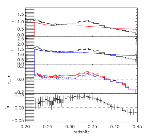
Figure 1: The observed and the predicted number and luminosity densities (first and second panel from the top, respectively). Number density in units of $10^{-4}$ Mpc${}^{-3}h^{3}$ and the luminosity density in arbitrary units and Mpc${}^{-3}h^{3}$. The observed values are in black, and the predicted values are in red for the number and blue for the luminosity densities. The shaded area shows the redshift range used to compute the predicted values. The third panel shows the loss rates in numbers (red) and luminosity (blue) given by Eqs. 9 and 10. Bottom: the galaxy luminosity loss rate given by Eq. 11. All rates are in Gyr^-1.

We begin by making no selection in luminosity, and comparing observed and predicted densities from galaxies with $\Delta z_{base}=[0.20,0.22]$ in the top two panels of Fig. 1. On the data side, we see a roughly constant number density from $z\approx 0.23$ to 0.33, an excess relative to this plateau at $z\lesssim 0.23$, a bump at $z\approx 0.34$, and a steep decline onwards. The roughly constant densities are a direct result of the targeting algorithm, which aimed to select LRGs up to a fixed number density by following a passively evolving stellar population. The fact that these are roughly constant can in itself put some constraints on the dynamical evolution of the sample (Wake et al., 2006, 2008). The excess at low redshift is likely to be contamination to the sample, where the target algorithm has less distinguishing power. The bump at $z\approx 0.34$ is a result of the widening colour cuts at that redshift, as we move from cut I to cut II in the target selection. The steep decline after that is dominated by the apparent magnitude cuts, with the decline in the observed number and luminosity densities being steeper than that predicted from the low redshift data.

The loss rates given by Eqs. 9 and 10 are shown on the third panel of Fig. 1, and we combine the information in all four observables to compute the merger rate, or galaxy luminosity loss rate, given by Eq. 11, which we show on the bottom panel of the same Figure. The merger rate is roughly constant and of the order of 3-4%, up to the point where the sample is dominated by the apparent magnitude limit.

In Fig. 2, we show how the predicted quantities change if we instead compute them from galaxies in different ranges $\Delta z_{base}$. Note that differences in the predicted quantities (in the blue and red lines) across the different plots provides information about the nature and evolution of the galaxies at each of the redshift intervals - this is discussed further in Section 6.

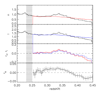
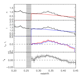
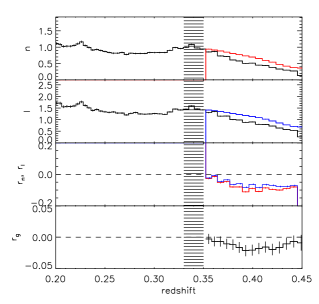
Figure 2: The same as Fig. 1, but exploring different intervals for $\Delta z_{base}$, used to compute the predicted quantities.

We can also investigate how the loss rates change with the magnitude of the galaxies. As all absolute magnitudes are K+e corrected, a flat cut in $M_{i}$ with redshift selects the same population of galaxies in the absence of mergers. In Fig. 3, we show how the observed and predicted quantities change when we restrict the analysis to galaxies with $M_{i}<-23$: this corresponds roughly to the top 30% brightest galaxies in the LRG sample. On the data side, we see many features in the redshift distributions disappear, leading to a flatter curve. The exception is at low redshift, where the excess in density is still present. We show the same redshift ranges of $\Delta z_{base}$ as explored in Figs. 1 and 2. Once again the observed curves are the same across all four panels, with differences in the red and blue curves holding information on the evolution of bright LRGs. We interpret and discuss these results in the next Section.

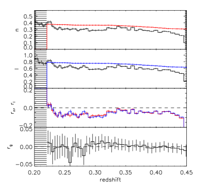
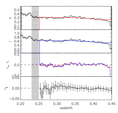
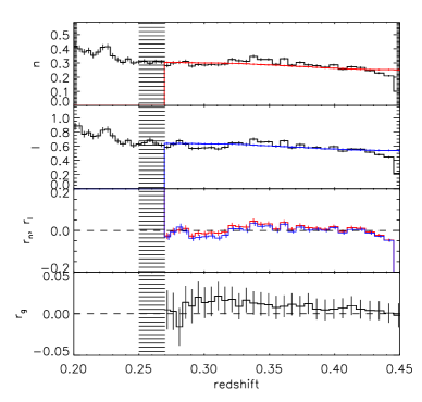
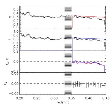
Figure 3: Same as Fig. 1, but using only galaxies with $M_{i}<-23$ and exploring different intervals for $\Delta z_{base}$, used to compute the predicted quantities.

5.1 Errors

The errors quoted throughout this paper are Poisson, and assume that our ability to compare predicted with observed quantities depends only how many objects we have available to do so. We account for the change in photometric errors using Eq. 4, which is folded into the predicted quantities.

It is particularly hard to estimate the effect of errors from the recovered star-formation histories on the computed merger rates. In T11 we presented an extensive analysis of the errors (see their Section 3.4), which we summarise here for completeness. There are two sources of errors that can affect the recovered star formation histories from VESPA: photon noise, which perturbs the spectra in way that we assume we understand; and systematic errors in models or parametrization, which are the result of our imperfect ability to correctly model certain stages of stellar evolution, chemical enrichment or dust extinction. The former is easily estimated, via a Monte Carlo approach that we explain in Tojeiro et al. (2009). In this case we are in the regime of extremely high signal-to-noise spectra and photon error is negligible. In order to understand systematic errors, in T11 we estimated these using the residuals of the best fit solution to the data (see their Fig. 3) - we found these errors to be at least 10 times larger. We use this error vector to obtain the SFHs used in the current analysis.

The effect of the uncertainties in the SFH on the measured rates comes from how many galaxies leave the survey’s selection window as a function of redshift, and how bright they are. The window function of the survey is designed to follow a passive evolution, so only star-formation histories that depart significantly from this model will affect the rates. An episode of recent to intermediate star formation of anything larger than 5% by mass is enough to take galaxies out of the survey box for up to and around 1Gyr (the exact number depends on the length of episode, the Stellar Population Synthesis (SPS) models used, the metallicity and the exact age of the burst) and, even though none of our formal error estimates allow for a discrepancy of this size, solutions obtained with different SPS models can differ by a few times this amplitude - we explicitly address the effect of using different SPS models in our results in Section 6.4.

The effect on the merger rate in turn depends on how many galaxies are removed from the sample. Our assumption in T11 is that all galaxies within a cell follow the SFH given by the stack that represents that cell. Each of our $\Delta z_{base}$ samples is typically represented by 4 to 12 stacks (depending on the luminosity range of the sample), and if one stack predicts a significant star-formation event ($\gtrsim$ 5% by mass), then 1/12 to 1/4 of the galaxies will be predicted to leave the sample for a significant period. This means that the effect on the merger rates are somewhat quantised, rather than a smooth function of an error in the SFHs. The effect can obviously be quite dramatic, and at its extreme it can predict that almost all galaxies would leave the sample, suggesting that the observed red sequence is an intricate combination of galaxies becoming red and blue throughout cosmic history (see Section 6.4 for an example).

6 Discussion

6.1 Interpreting the observables

If the sample of SDSS-II LRGs was not affected by mergers, and assuming the SFHs are correct (see Section 5.1), then the observed luminosity and the number densities would obviously match the extrapolated values. Any deviations from this, implies merger activity and/or a non-zero net flow of galaxies into the sample. We cannot determine a balance between mergers into and out of the sample. However, by comparing number and luminosity evolution we can start to understand the evolution that we do see.

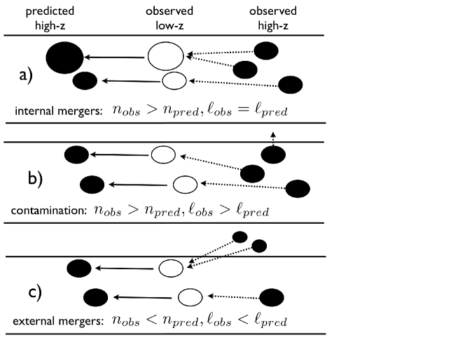
Figure 4: Diagram of possible interpretations for discrepancies in the observed and predicted quantities. The middle column shows the observed luminosity and number densities. The solid arrows show the prediction given by the stellar evolution from VESPA and the survey’s window function, and they lead to the left hand side column that shows the predicted luminosity and number densities. Note that whereas VESPA can only predict changes in the luminosity density, the window function can also affect the number densities. The window function is fully known and introduces no ambiguity when computing the predicted quantities - in here we show the numbers being conserved just for simplicity. The right hand side column shows the observed number and luminosity densities, and the dotted arrows represent our proposed interpretation. See Section 6.1 for more details.

Fig. 4 shows schematically the simplest interpretation for three scenarios:

1. $n_{pred}<n_{obs}$ and $\ell_{pred}=\ell_{obs}$ - the simplest interpretation is that galaxies within the sample have merged together to decrease the predicted number density of objects, whilst retaining the sample luminosity. This assumes no luminosity loss to the intra-cluster medium.

2. shows how contamination from objects at a given redshift could also act to give $n_{pred}<n_{obs}$ in the same way as internal mergers. By contaminants here we refer to objects that would enter the sample for a short time only, and do not evolve to be present in the sample at low redshift. However, the comparison between $\ell_{obs}$ and $\ell_{pred}$ helps to differentiate the two scenarios, as in this case we expect the excess in the observed number density due to contamination to be matched by an excess of luminosity density. The two excesses will be matched in amplitude provided the contaminants have the same luminosity function as the galaxies that evolve through the sample.

3. $n_{pred}>n_{obs}$ and $\ell_{pred}>\ell_{obs}$. This scenario requires an enrichment of the sample towards lower redshift - either by the merging of fainter galaxies becoming brighter and crossing over the faint magnitude cuts, bluer galaxies turning redder and crossing over the colour cuts, or a combination of both.

Note that in the case of fainter galaxies merging together to become brighter and entering the sample by crossing over the magnitude cuts, scenarios (a) and (c) represent the same physical process - the only difference between is where the survey’s magnitude cut lies. We explore this fact in a little more detail in Section 6.3.

Obviously, we can expect multiple scenarios such as those in Fig. 4 to happen simultaneously. If this is the case, under the assumption that the luminosity function of the contaminants matches that of the objects in the sample, and that luminosity is conserved in a merger event, Eq. 11 gives the best estimate for the merger rate required for galaxies within the sample between $\Delta z$ and $\Delta z_{base}$. In fact, even if these assumptions are broken, Eq. 11 still acts as a lower limit on the true merger rate. This is mostly easily seen from Equation (11) - we are effectively under-estimating $\ell_{pred}$, as some luminosity has been lost to the intracluster medium, resulting in an under-estimation of $r_{g}$.

6.2 Interpreting the results

Using the results of Section 5, we can identify redshift intervals that are likely to be dominated by each of the scenarios shown in Fig. 4. Starting with the results for all LRGS, shown in Fig. 1, we see the predicted number and luminosity densities both fall short of the observed values up to $z\approx 0.38$, suggesting a combination of scenarios (a) and (b). The bump at $z\approx 0.34$ is not reproduced by the stellar evolution of present-day galaxies, strongly suggesting that is it caused by contamination of galaxies as the colour cuts widen - in other words, the wider breadth of colour in the sample at those redshifts is not predicted by the stellar evolution of more local galaxies. Therefore the signal here is likely dominated by scenario (b). Finally, the sample of local galaxies predicts a much shallower slope in the number densities as we go towards higher redshifts, suggesting that they were still being assembled (in a dynamical sense) at those epochs - in other words, had the local galaxies still be in one piece at $z\gtrsim 0.4$ they would have been bright enough to be in the sample. This puts us in a regime likely to be dominated by scenario (c) at these high redshifts.

Moreover, at the high-redshift tail where scenario (c) dominates, we note that the number loss rate is higher (in amplitude) than the luminosity loss rate. In other words, the typical luminosity per object at $z\gtrsim 0.38$ is lower than expected. This suggests that the LRG growth due to external merging is happening predominantly at the fainter end of the sample. We will investigate this hypothesis further in Section 6.2.2. Note that if this growth was constant with luminosity then both loss rates would have a negative value, but would be matched in amplitude - resulting in a zero galaxy luminosity loss rate, interpreted in this case as a zero internal merger rate.

6.2.1 Changing $\Delta z_{base}$

We now consider the effect of changing the low redshift intervals $\Delta z_{base}$, from which we infer the galaxy evolution from high redshift as shown in Fig. 2. Changes in the inferred loss and merger rates as we change our low-redshift sample are sensitive to differences in the low redshift population of galaxies.

We find no significant difference in the evolution of galaxies observed between $z=0.23$ and $z=0.27$ - see the first two panels of Fig. 2 - but comparing the rate of luminosity loss per galaxy (lower panels in the figures) to those in Fig. 1 suggests that the lower redshift galaxies experience a more pronounced growth. This is consistent with a hypothesis in which the low redshift end of the sample is not as pure as the rest of the sample - the targeting algorithm is less robust at these redshifts (Eisenstein et al., 2001; Tojeiro et al., 2011). Furthermore, the sample will naturally be more enriched towards fainter galaxies, which could have a different growth rate - see Section 6.2.2 for more details.

Similarly, galaxies observed at redshifts between $0.33$ and $0.35$ are seen to have a different growth compared with galaxies at lower redshifts. This is not unexpected, as the bump in number and luminosity density at $z\approx 0.34$ is not predicted by galaxies at low redshifts. These results suggest that the wider colour selection of cut II selects galaxies not only with a different stellar evolution, but also a different merger growth rate - essentially a different population of galaxies. For the same reasons as before, we argue that this growth must be happening predominantly at the faint end.

6.2.2 Changing the luminosity

In Fig. 3 we restrict our analysis to galaxies with a K+e corrected M${}_{i}<-23$, which corresponds roughly to the brightest third of the galaxies in the sample. We show results for the same four ranges of $\Delta z_{base}$ as before. It is immediately clear that a lot of the features in the observed quantities are less pronounced - the bump at $z\approx 0.34$ almost disappears, and the high-redshift tail flattens out as we restrict ourselves to what is close to magnitude-limited sample (colour cuts excluded). The exception is the bump at low redshifts, which, combined with the measured loss and merger rates for $\Delta z_{base}=[0.20,0.22]$, suggests the luminous galaxies observed at low redshift are still growing, and this growth is approximately matches that of lower luminosity objects. Clearly this also fits with the hypothesis that the lower redshift galaxies form a population with more dynamical evolution than the higher redshift galaxies within the sample.

For all other cases of $\Delta z_{base}$ we find a picture that is consistent with passive dynamical growth, with the only - and marginal - evidence for external growth coming for the galaxies in $\Delta z_{base}=[0.33,0.35]$, perhaps suggesting that not even the brightest galaxies are purely coeval across the two LRG colour cuts described in Section 2.

6.3 Probing the typical luminosity of mergers

We noted in Section 6.1 that scenarios (a) and (c) represent the same physical merger process, but can be distinguished as (c) caused objects to cross the apparent magnitude cut on the sample. In Section 6.2, we suggested than (c) dominates at high redshift, while (a) dominates at low redshift. We can use the information available to define a typical luminosity for the dominant merger process happening.

For each case of $\Delta z_{base}$ we take the redshift at which the number and luminosity loss rates cross the zero line and compute the absolute magnitude that would correspond to the apparent petrosian magnitude equal to the survey’s limit of $r_{p}=19.5$ - in other words, the faintest absolute magnitude observed at that redshift. These are the galaxies that are beginning to enter the sample when dynamical growth transitions from external to internal. Note that the two growth rates change sign at very similar epochs, so we can use either without significant effect on our results. In Fig. 5 we show how this transitional absolute magnitude changes for the four different cases of $\Delta z_{base}$ (those shown in Figs. 1 and 2).

Figure 5: The dots show the transitional absolute magnitude as a function of $\Delta z_{base}$ (on the right-hand side y-axis) - see Section 6.3. This is the absolute $r-band$ magnitude that corresponds to the $r_{p}=19.5$ cut on petrosian magnitude of cut II (Eisenstein et al., 2001) at the redshifts for which we infer a transition from external to external growth. For context we also show the distribution of absolute magnitudes of galaxies in the sample (on the left-hand side y-axis).

Once again our result is that the dynamical growth is happening predominantly at the faint end, for galaxies observed in all the four intervals of $\Delta z_{base}$ we studied.

6.4 Robustness to SPS models

In Tojeiro et al. (2011) we showed how the measured stellar evolution of LRGs depends on the SPS models used - see Fig. 6 in that paper for a summary of the differences. The results presented in this paper thus far assume the stellar and colour evolution given by the Flexible Stellar Population Synthesis (FSPS) models of Conroy et al. (2009); Conroy & Gunn (2010), which gave better fits to the spectral data and resulted in the more passive stellar evolution model in our previous study. However, as we could not conclusively decide which set of SPS models gives a more accurate description of the real stellar evolution of LRGs, in this section we discuss how the stellar evolution given by other models would change the interpretation given above. The results on the recovered merger rate and interpretation of the dynamical evolution can be dramatically affected by events of star formation.

In the case of the Maraston et al. 2011 models (M10, submitted), the amount of recent to intermediate star formation dominates only in galaxies at $z\lesssim 0.3$. The resulting interpretation is that contamination of the LRG sample extends to a larger redshift than what would be assumed using the FSPS models, and that these local galaxies are not the evolutionary products of the LRGs observed at higher redshifts. At $z>0.3$, however, the recovered dynamical evolution is qualitatively similar to that obtained with the FSPS models, although with slightly larger rates.

The interpretation using the stellar evolution given by the models of Bruzual & Charlot (2003) (BC03), however, is incompatible with the hypothesis that the LRGs form a coeval population of galaxies since $z<0.45$. The significant and continuous (with redshift) amount of recent to intermediate star formation lead to a consistently under-prediction of the number and luminosity densities at high redshifts from more local samples, in a way that is only explained by a continuous amount of contamination in the sample.

6.5 Comparison with previous results

The results in this paper are in qualitative agreement with those in Tojeiro & Percival (2010), where we used the luminosity weighted power-spectrum to argue that the LRG population is growing via external mergers at the faint end. Quantitatively, however, the rates we find in this paper are lower by roughly a factor of two. The main difference between the two approaches lies on the treatment of the stellar evolution - whilst in Tojeiro & Percival (2010) we assumed that the passive stellar evolution model of Maraston et al. (2009) was suitable for all galaxies in the sample, in here we instead use the stellar evolution models of Tojeiro et al. (2011) which use the fossil record of LRGs of different colour, luminosity and redshift to infer the most-likely stellar evolution. Furthermore, in Tojeiro & Percival (2010), we assumed that the scatter in colour and magnitude was due to intrinsic or photometric errors, which is a byproduct of assuming that all LRGs in the sample share the same stellar evolution. Instead, the analysis presented in this paper makes no such assumption, and is robust to an influx and/or an outflux of objects if we interpret the measured rates as a lower limit. It is the independent treatment of the stellar evolution, and the detailed comparison of predicted with observed quantities that allows us to make an assessment on the nature of the mergers without the need for a clustering analysis.

Comparisons with other works is less trivial, due to the typically different samples used. We refer the reader to Section 8 of Tojeiro & Percival (2010) for a summary of recent results and comparison. We continue to argue that merging at the faint end of the LRG population is a more likely explanation published for the published evidence for both luminosity growth (Brown et al., 2007; White et al., 2007; Cool et al., 2008; Masjedi et al., 2008) and loss of number density (Masjedi et al., 2006; Wake et al., 2006; White et al., 2007; Wake et al., 2008; De Propris et al., 2010).

7 Summary and conclusions

In this paper we have demonstrated how we can use the fossil record of galaxies to extrapolate from low redshift samples to match samples selected at higher redshift. By comparing against the observed number and luminosities, we can measure growth and consider where the dynamical evolution of galaxies is required. We have applied this technique to consider the dynamical evolution of galaxies in the SDSS-II LRG sample, although the technique could be used to link different surveys at low and high redshift.

For the SDSS-II LRG sample, we have previously predicted the stellar evolution in Tojeiro et al. (2011), by using the fossil record encoded in the spectra of LRGs. This allowed us to compute the most likely stellar evolution of observed LRGs in a way that was decoupled from the survey’s selection function. We used this information to make predictions on the number and luminosity of LRGs at higher redshift from a local sample of galaxies, and we showed how differences in these quantities can be interpreted as a minimum merger rate. Our main conclusions can be summarised as the two following points:

• the LRG population is not purely coeval, with some of galaxies targeted at $z<0.22$ and at $z>0.34$ showing different dynamical growth than galaxies targeted throughout the sample;

• the LRG population is still dynamically growing, and this growth must be limited to the faint end;

Based on these results, we argue that a coeval population of galaxies that has been dynamically passive to less than 1-2% can be robustly selected from the LRG sample, by imposing a cut on the K+e corrected absolute magnitude, and by selecting galaxies with $z\in[0.23,0.45]$. This merger rate is lower than those previously measured by roughly a factor of two, because, by using empirically determined evolutionary tracks we no longer need to assume passive evolution, and this previously led to incorrect evolutionary tracks for some galaxies.

We caution against interpreting these results beyond the limits of the stellar population models, and once again stress the important of good models and statistically good fits for analyses of this type. However, given the power inherent in the type of approach, and improvements in SPS modelling due in the future, we consider this analysis to be a forerunner of significant future work.

8 Acknowledgments

We thank the anonymous referee for a report that helped us clarify a number of issues. We thank David Wake for helpful discussions and encouragement. RT thanks Alan Heavens and Raul Jimenez for help in the development of VESPA. RT thanks the Leverhulme trust for financial support. WJP is grateful for support from the UK Science and Technology Facilities Council (grant ST/I001204/1), the Leverhulme trust and the European Research Council.

Funding for the SDSS and SDSS-II has been provided by the Alfred P. Sloan Foundation, the Participating Institutions, the National Science Foundation, the U.S. Department of Energy, the National Aeronautics and Space Administration, the Japanese Monbukagakusho, the Max Planck Society, and the Higher Education Funding Council for England. The SDSS Web Site is http://www.sdss.org/.

References

- Abazajian et al. (2009) Abazajian K. N., et al., 2009, ApJ Supplement Series, 182, 543
- Brown et al. (2007) Brown M. J. I., Dey A., Jannuzi B. T., Brand K., Benson A. J., Brodwin M., Croton D. J., Eisenhardt P. R., 2007, ApJ, 654, 858
- Bruzual & Charlot (2003) Bruzual G., Charlot S., 2003, MNRAS, 344, 1000
- Cappellari et al. (2009) Cappellari M., di Serego Alighieri S., Cimatti A., Daddi E., Renzini A., Kurk J. D., Cassata P., Dickinson M., Franceschini A., Mignoli M., Pozzetti L., Rodighiero G., Rosati P., Zamorani G., 2009, ApJL, 704, L34
- Conroy & Gunn (2010) Conroy C., Gunn J. E., 2010, ApJ, 712, 833
- Conroy et al. (2009) Conroy C., Gunn J. E., White M., 2009, ApJ, 699, 486
- Cool et al. (2008) Cool R. J., Eisenstein D. J., Fan X., Fukugita M., Jiang L., Maraston C., Meiksin A., Schneider D. P., Wake D. A., 2008, ApJ, 682, 919
- De Propris et al. (2010) De Propris R., Driver S. P., Colless M., Drinkwater M. J., Loveday J., Ross N. P., Bland-Hawthorn J., York D. G., Pimbblet K., 2010, AJ, 139, 794
- Drory & Alvarez (2008) Drory N., Alvarez M., 2008, ApJ, 680, 41
- Drory et al. (2005) Drory N., Salvato M., Gabasch A., Bender R., Hopp U., Feulner G., Pannella M., 2005, ApJL, 619, L131
- Eisenstein et al. (2001) Eisenstein D. J., et al., 2001, AJ, 122, 2267
- Eskew & Zaritsky (2011) Eskew M., Zaritsky D., 2011, AJ, 141, 69
- Gunn et al. (1998) Gunn J. E., et al., 1998, AJ, 116, 3040
- Komatsu et al. (2011) Komatsu E., et al., 2011, ApJ Supplement Series, 192, 18
- Maraston et al. (2009) Maraston C., Strömbäck G., Thomas D., Wake D. A., Nichol R. C., 2009, MNRAS, 394, L107
- Masjedi et al. (2008) Masjedi M., Hogg D. W., Blanton M. R., 2008, ApJ, 679, 260
- Masjedi et al. (2006) Masjedi M., Hogg D. W., Cool R. J., Eisenstein D. J., Blanton M. R., Zehavi I., Berlind A. A., Bell E. F., Schneider D. P., Warren M. S., Brinkmann J., 2006, ApJ, 644, 54
- Naab et al. (2009) Naab T., Johansson P. H., Ostriker J. P., 2009, ApJL, 699, L178
- Percival et al. (2010) Percival W. J., et al., 2010, MNRAS, 401, 2148
- Percival et al. (2007) Percival W. J., Nichol R. C., Eisenstein D. J., Weinberg D. H., Fukugita M., Pope A. C., Schneider D. P., Szalay A. S., Vogeley M. S., Zehavi I., Bahcall N. A., Brinkmann J., Connolly A. J., Loveday J., Meiksin A., 2007, ApJ, 657, 51
- Reid et al. (2010) Reid B. A., et al., 2010, MNRAS, 404, 60
- Saracco et al. (2011) Saracco P., Longhetti M., Gargiulo A., 2011, MNRAS, 412, 2707
- Stoughton et al. (2002) Stoughton C., et al., 2002, AJ, 123, 485
- Tojeiro et al. (2007) Tojeiro R., Heavens A. F., Jimenez R., Panter B., 2007, MNRAS, 381, 1252
- Tojeiro & Percival (2010) Tojeiro R., Percival W. J., 2010, MNRAS, 405, 2534
- Tojeiro et al. (2011) Tojeiro R., Percival W. J., Heavens A. F., Jimenez R., 2011, arXiV:1011.2346
- Tojeiro et al. (2009) Tojeiro R., Wilkins S., Heavens A. F., Panter B., Jimenez R., 2009, ApJ Supplement Series, 185, 1
- van Dokkum et al. (2008) van Dokkum P. G., et al., 2008, ApJL, 677, L5
- Wake et al. (2006) Wake D. A., et al., 2006, MNRAS, 372, 537
- Wake et al. (2008) Wake D. A., et al., 2008, MNRAS, 387, 1045
- White et al. (2007) White M., Zheng Z., Brown M. J. I., Dey A., Jannuzi B. T., 2007, ApJL, 655, L69
- White & Rees (1978) White S. D. M., Rees M. J., 1978, MNRAS, 183, 341
- York et al. (2000) York D. G., et al., 2000, AJ, 120, 1579