Illustrating the Geometry of Coherently Controlled
Unital Open Quantum Systems

Zusammenfassung

We extend standard Markovian open quantum systems (quantum channels) by allowing for Hamiltonian controls and elucidate their geometry in terms of Lie semigroups. For standard dissipative interactions with the environment and different coherent controls, we particularly specify the tangent cones (Lie wedges) of the respective Lie semigroups of quantum channels. These cones are the counterpart of the infinitesimal generator of a single one-parameter semigroup. They comprise all directions the underlying open quantum system can be steered to and thus give insight into the geometry of controlled open quantum dynamics. Such a differential characterisation is highly valuable for approximating reachable sets of given initial quantum states in a plethora of experimental implementations.

I Introduction

Extending quantum channels by allowing for Hamiltonian control turns them into interesting and important examples of geometric control of open systems. While for closed systems, the theory of Lie groups provides a rich structure to address questions of reachability, accessibility, and controllability [1], already simple open quantum systems come with the intricate geometry of Lie semigroups [2, 3]. For instance, in most closed systems the reachable set to an initial state $\rho_{0}$ simply is the orbit $\mathcal{O}_{\textbf{G}}(\rho_{0}):=\{G\rho_{0}G^{-1}\,|\,G\in\textbf{G}\}$ of a unitary subgroup G whose Lie algebra can be identified easily via Lie closure, while in open systems reachable sets are much more difficult to determine explicitly. Thus in view of controlling open quantum dynamics, in [4] we systematically related the framework of completely positive semigroups [5, 6, 7, 8, 9, 10, 11], which is well established in quantum physics, with the more recent mathematical theory of Lie semigroups. An early example confined to single-qubit systems can be found in [12].

More precisely, for exploiting the power of systems and control theory in open quantum dynamics, the system parameters have to be characterised first, e.g., by input-output relations in the sense of quantum process tomography. The decision problem whether the dynamics of the quantum system thus specified is Markovian to good approximation has recently been analysed [13, 14]. Moreover (time-dependent) Markovian quantum channels were elucidated from the viewpoint of divisibility [13] thus paving the way to Lie semigroups [4]. Following up, this work sets out to determine the geometry of quantum channel semigroups in terms of their tangent cones (Lie wedges) for a number of coherently controlled standard unital channels in a unified frame in line with [15].

For the first time, here we explicitly parameterize the set of all possible directions an open quantum system under coherent controls may take — its Lie wedge. Thereby, we heavily exploit the fact that the set of all reachable quantum maps governed by a controlled Markovian master equation constitutes a Lie semigroup [4]. Previous characterizations of reachable sets for unital open quantum systems by majorization techniques, e.g., [16], become increasingly inaccurate once full controllability of the Hamiltonian part (condition (H) vide infra) is violated, which for growing number of qubits happens in all experimentally realistic settings. In contrast, the Lie-semigroup tools presented here do not require condition (H) and carry over to multi-qubit systems without the draw-back of increasing inaccuracy.

II Theory and Background

We start out by recalling some basic notions and notations of Lie subsemigroups [2] and their application for characterising reachable sets of quantum control systems modelled by Lindblad-Kossakowski master equations [4].

II-A Lie Semigroups

To begin with, let G be a matrix Lie group, i.e. a group which is (isomorphic to) a path-connected subgroup of $GL(n,\mathbb{R}^{\,}{})$ or $GL(n,\mathbb{C}^{\,}{})$ for some $n\in\mathbb{N}{}{}$, and let $\mathfrak{g}$ be its corresponding matrix Lie algebra. Thus $\mathfrak{g}$ is (isomorphic to) a Lie subalgebra of $\mathfrak{gl}(n,\mathbb{R}^{\,}{})$ or $\mathfrak{gl}(n,\mathbb{C}^{\,}{})$. Then a subset $\textbf{S}\subset\textbf{G}$ which is closed under the group operation in the sense $\textbf{S}\cdot\textbf{S}\subseteq\textbf{S}$ and which contains the identity ${\rm 1\negthickspace l}{}$ is said to be a subsemigroup of G. The largest subgroup within S is written $E(\textbf{S}):=\textbf{S}\cap\textbf{S}^{-1}$.

Furthermore, a closed convex cone $\mathfrak{w}\subset\mathfrak{g}$ is called a wedge. The largest linear subspace of $\mathfrak{w}$ is denoted $E(\mathfrak{w}):=\mathfrak{w}\cap(\mathfrak{-w})$ and it is termed the edge of the wedge $\mathfrak{w}$. Now, $\mathfrak{w}\subseteq\mathfrak{g}$ is a Lie wedge of $\mathfrak{g}$ if it is invariant under the adjoint action of the subgroup generated by the edge $E(\mathfrak{w})$, i.e. if it satisfies

$$e^{A}\,\mathfrak{w}\,e^{-A}=\mathfrak{w}$$ (1)

(or equivalently $e^{\operatorname{ad}_{A}}(\mathfrak{w})=\mathfrak{w}$) for all $A\in E(\mathfrak{w})$. Note that the edge of a Lie wedge always forms a Lie subalgebra of $\mathfrak{g}$.

Moreover, for any closed subsemigroup S of G we define its tangent cone $L(\textbf{S})$ at the identity ${\rm 1\negthickspace l}{}$ by

$$L(\textbf{S}):=\{A\in\mathfrak{g}\,|\,\exp(tA)\in\textbf{S}\text{\; for all\;}t\geq 0\}\;.$$ (2)

Then one can show that $L(\textbf{S})$ is a Lie wedge of $\mathfrak{g}$ satisfying the identity $E\big{(}L(\textbf{S})\big{)}=L\big{(}E(\textbf{S})\big{)}.$ Yet, the ‘local-to-global’ correspondence between Lie wedges and closed connected subsemigroups is much more subtle than the correspondence between Lie (sub)algebras and Lie (sub)groups: for instance, several connected subsemigroups may share the same Lie wedge $\mathfrak{w}$ in the sense that $L(\textbf{S})=L(\textbf{S}^{\prime})$ for $\textbf{S}\neq\textbf{S}^{\prime}$, or conversely there may be Lie wedges $\mathfrak{w}$ which do not correspond to any subsemigroup, i.e. $\mathfrak{w}=L(\textbf{S})$ fails for all subsemigroups $\textbf{S}\subset\textbf{G}$.

Therefore, one introduces the important notion of a Lie subsemigroup S which is characterised by the equality

$$\textbf{S}=\overline{\langle\exp L(\textbf{S})\rangle{}}_{S}\;,$$ (3)

where the closure is taken in G and $\langle\exp L(\textbf{S})\rangle{}_{S}$ denotes the subsemigroup generated by $\exp L(\textbf{S})$, i.e. $\langle\exp L(\textbf{S})\rangle{}_{S}:=\{e^{A_{1}}\cdots e^{A_{n}}\,|\,n\in\mathbb{N}{},\,A_{1},\dots,A_{n}\in L(\textbf{S})\}$. Moreover, a Lie wedge $\mathfrak{w}$ is said to be global in G, if there is a Lie subsemigroup $\textbf{S}\subset\textbf{G}$ such that

$$L(\textbf{S})=\mathfrak{w}\;.$$ (4)

Thus, one has the identity $\textbf{S}=\overline{\langle\exp\mathfrak{w}\rangle{}}_{S}$.

Whenever a Lie wedge $\mathfrak{w}\subset\mathfrak{g}$ specialises to be compatible with the Baker-Campbell-Hausdorff (BCH) multiplication

$$A\star B:=A+B+\tfrac{1}{2}[A,B]+\dots=\log(e^{A}e^{B})\quad\forall A,B\in\mathfrak{w}$$ (5)

defined via the BCH series, it is termed Lie semialgebra. For this to be the case, there has to be an open BCH neighbourhood $\mathcal{B}\subset\mathfrak{g}$ of the origin in $\mathfrak{g}$ such that $(\mathfrak{w}\cap\mathcal{B})\star(\mathfrak{w}\cap\mathcal{B})\subseteq\mathfrak{w}$. An equivalent definition for being a Lie semialgebra is given by the tangential condition

$$[A,T_{A}\mathfrak{w}]\subset T_{A}\mathfrak{w}\quad\text{for all $A\in\mathfrak{w}$}\;,$$ (6)

where $T_{A}\mathfrak{w}$ denotes the tangent space of $\mathfrak{w}$ at $A$ defined by

$$T_{A}\mathfrak{w}:=\big{(}A^{\perp}\cap\mathfrak{w}^{*}\big{)}^{\perp}\;.$$ (7)

Here $A^{\perp}$ denotes the orthogonal complement of $A$ and $\mathfrak{w}^{*}:=\{A\in\mathfrak{g}\,|\,\langle A,B\rangle\geq 0\text{ for all }B\in\mathfrak{w}\}$ the dual wedge—both taken with respect to the standard trace inner product. The conceptual importance of Lie semialgebras roots in the fact that—in Lie semialgebras—the exponential map of a zero-neighbourhood in $L(\textbf{S})$ yields a ${\rm 1\negthickspace l}{}$-neighbourhood in S. In contrast, as soon as $\mathfrak{w}$ is merely a Lie wedge that fails to carry the stronger structure of a Lie semialgebra, there will be elements in S that are arbitrary close to the identity without belonging to any one-parameter semigroup completely contained in S. For more details and a variety of illustrative examples, we recommend [2] and [17], where the respective introduction does provide a lucid overview of the entire subject. The connection between Lie semialgebras and time-independent Markovian quantum channels has been worked out in detail in [4].

With these stipulations, the frame is set to describe the time evolution of Markovian (i.e., memory-less) open quantum systems in the differential geometric picture of Lie wedges.

II-B Markovian Quantum Dynamics and Quantum Channels

Markovian quantum dynamics is conveniently described by a linear autonomous differential equation

$$\dot{X}(t)=-\mathcal{L}\,X(t)\;,$$ (8)

where $X(t)$ usually denotes the state of a quantum system represented by its density operator $\rho(t)$, i.e. $\rho(t)=\rho(t)^{\dagger}$, $\rho(t)\geq 0$, and $\operatorname{tr}\rho(t)=1$. Here and henceforth, $(\cdot)^{\dagger}$ denotes the adjoint (complex-conjugate transpose). For ensuring complete positivity, $\mathcal{L}$ has to be of Lindblad form [10], i.e.

$$\mathcal{L}(\rho)=i\operatorname{ad}_{H}(\rho)+\Gamma_{L}(\rho)\;,$$ (9)

with $\operatorname{ad}_{H_{j}}(\rho):=[H_{j},\rho]$ and

$$\Gamma_{L}(\rho):=\tfrac{1}{2}\sum_{k}V_{k}^{\dagger}V_{k}\rho+\rho V_{k}^{\dagger}V_{k}-2V_{k}\rho V_{k}^{\dagger}\;,$$ (10)

Here, the Hamiltonian $H$ is assumed to be a Hermitian $N\times N$ matrix while the Lindblad generators $\{V_{k}\}$ may be arbitrary $N\times N$ matrices. The resulting equation of motion (8) acts on the vector space of all Hermitian operators, $\mathfrak{her}{}(N)$, and more precisely, leaves the set of all density operators $\mathfrak{pos}{}_{1}(N):=\left\{\rho\in\mathfrak{her}{}(N)\,|\,\rho=\rho^{\dagger},\rho\geq 0,\operatorname{tr}\rho=1\right\}$ invariant.

In [4] it was shown that the set of all Lindblad generators $\{-\mathcal{L}\}$ has an interpretation as a particular Lie wedge. To see this, consider the group lift of (8), i.e. now $X(t)$ denotes an element in the general linear group $GL(\mathfrak{her}{}(N))$. Moreover, define the set of all completely positive (cp), trace-preserving invertible linear operators acting on $\mathfrak{her}{}(N)$ as $\textbf{P}^{cp}$, i.e.

$$\textbf{P}^{cp}:=\{T\in GL(\mathfrak{her}{}(N))\,|\,T\;\text{is cp and trace-preserving}\}$$

and let $\textbf{P}^{cp}_{0}$ denote its connected component of the identity. Then, $\textbf{P}^{cp}$ is exactly the set of so-called invertible quantum channels. A quantum channel $T$ is said to be time independent Markovian or briefly Markovian, if it is a solution of (8). Thus $T={\rm e}^{-t\mathcal{L}}$ for some fixed Lindblad generators $\mathcal{L}$ and some $t\geq 0$. Furthermore, $T$ is time dependent Markovian if it is a solution of (8), where now $\mathcal{L}=\mathcal{L}(t)$ may vary in time (for terminology see also [13, 14]). Finally, we will denote the set of all time independent Markovian and time dependent Markovian quantum channels by $\mathbf{MQC}$ and $\mathbf{TMQC}$, respectively. Then, with regard to the work by Lindblad [10] and Kossakowski [9], one obtains the following result [4]:

1. The global Lie wedge of $\textbf{P}^{cp}_{0}$ is given by the set of all Lindblad generators of the form

   $$-\mathcal{L}:=-\big{(}i\operatorname{ad}_{H}+\Gamma_{L}\big{)}$$ (11)

   with $H\in\mathfrak{her}{}(N)$ and $\Gamma_{L}$ as in (10).

2. The Lie semigroup

   $$\overline{\langle\exp L(\textbf{P}^{cp}_{0})\rangle{}}_{S}$$ (12)

   clearly contains $\mathbf{MQC}$ and moreover it exactly coincides with the closure of $\mathbf{TMQC}$ thus excluding the non-Markovian ones in $\textbf{P}^{cp}_{0}$, which is most remarkable.

While assertion (a) reformulates previous results by Lindblad and Kossakowski [6, 9, 10], part (b) is noteworthy as it also says that $\textbf{P}^{cp}_{0}$ is not a Lie subsemigroup of $GL(\mathfrak{her}{}(N))$.

II-C Coherently controlled Master Equations

Controlled Markovian quantum dynamics is appropriately addressed as right-invariant bilinear control system [4, 18, 19, 20]

$$\dot{\rho}(t)=-\mathcal{L}_{u(t)}\big{(}\rho(t)\big{)}\quad,\quad\rho(0)\in\mathfrak{pos}{}_{1}(N)\;,$$ (13)

where $\mathcal{L}_{u}$ now depends on some control variable $u\in\mathbb{R}^{\,}{}^{m}$.

Here, we focus on coherently controlled open systems. This means that $\mathcal{L}_{u}$ has the following special from

$$\mathcal{L}_{u}(\rho)=-i\operatorname{ad}_{H_{u}}(\rho)-\Gamma_{L}(\rho)\quad\text{with}$$ (14)

$$\operatorname{ad}_{H_{u}}:=\operatorname{ad}_{H_{d}}+\sum_{j=1}^{m}u_{j}\operatorname{ad}_{H_{j}}\;.$$ (15)

Note that the control terms $i\operatorname{ad}_{H_{j}}$ with control Hamiltonians $H_{j}\in\mathfrak{her}{}(N)$ are usually switched by piecewise constant control amplitudes $u_{j}(t)\in\mathbb{R}^{\,}{}$. The drift term of (14) is then composed of two parts, (i) the term $i\operatorname{ad}_{H_{d}}$ (in abuse of language sometimes called ‘Hamiltonian’ drift) accounting for the coherent time evolution and (ii) a dissipative Lindblad part $\Gamma_{L}$. So $\mathcal{L}_{u}$ denotes the coherently controlled Lindbladian. As in the uncontrolled case, system (13) acts on the vector space of all Hermitian operators leaving the set of all density operators invariant. Equivalently, one can regard (13) as an affine system on $\mathfrak{her}_{0}(N):=\{H\in\mathfrak{her}{}(N)\;|\;\operatorname{tr}H=0\}$.

In the following, we further impose unitality, i.e. we assume $\Gamma_{L}({\rm 1\negthickspace l}{})=0$. This ensures that (13) actually yields a bilinear control system on $\mathfrak{her}_{0}(N)$ instead of an affine one. Therefore, it allows a group lift to $GL\big{(}\mathfrak{her}_{0}(N)\big{)}$ which henceforth is referred to as ($\Sigma$), i.e.

$$(\Sigma)\quad\dot{X}(t)=-\mathcal{L}_{u(t)}\,X(t)\,,\;X(0)\in GL\big{(}\mathfrak{her}_{0}(N)\big{)}\;.$$ (16)

The corresponding group lift in the affine case is more involved [19, 4]. Now, the system semigroup $\textbf{P}_{\Sigma}$ associated to ($\Sigma$) reads

$$\textbf{P}_{\Sigma}=\langle T_{u}(t)=\exp(-t\mathcal{L}_{u})\,|\,t\geq 0,u\in\mathbb{R}^{\,}{}^{m}\rangle_{S}$$ (17)

and lends itself to exemplify the notion of a Lie wedge. To distinguish between different notions of controllability in open systems, we define three algebras: the control algebra $\mathfrak{k}_{c}$, the extended algebra $\mathfrak{k}_{d}$, and the system algebra $\mathfrak{s}$ as follows

$$\begin{split}\mathfrak{k}_{c}&:=\langle i\operatorname{ad}_{H_{j}}\,|\,j=1,\dots,m\rangle{}_{\sf Lie}\;,\\[5.69054pt] \mathfrak{k}_{d}&:=\langle i\operatorname{ad}_{H_{d}},i\operatorname{ad}_{H_{j}}\,|\,j=1,\dots,m\rangle{}_{\sf Lie}\;,\\[5.69054pt] \mathfrak{s}&:=\langle\mathcal{L}_{u}|\,u_{j}\in\mathbb{R}\rangle{}_{\sf Lie}\\[5.69054pt] &=\langle i\operatorname{ad}_{H_{d}}+\Gamma_{L},i\operatorname{ad}_{H_{j}}|\,j=1,\dots,m\rangle{}_{\sf Lie}\;.\end{split}$$ (18)

Note that $\mathfrak{s}$ is different from $\mathfrak{k}_{d}$, because it contains the entire drift term $(i\operatorname{ad}_{H_{d}}+\Gamma_{L})$ for the Lie closure, while $\mathfrak{k}_{d}$ only takes its Hamiltonian component $i\operatorname{ad}_{H_{d}}$. Then $(\Sigma)$ is said to fulfill condition (H), (WH), and (A), respectively, if

$$(H)\qquad\mathfrak{k}_{c} =\;\operatorname{ad}_{\mathfrak{su}(N)}$$ (19)

$$(W\negthinspace H)\quad\mathfrak{k}_{d} =\;\operatorname{ad}_{\mathfrak{su}(N)}\;\text{while}\;\;\mathfrak{k}_{c}\neq\operatorname{ad}_{\mathfrak{su}(N)}$$ (20)

$$(A)\qquad\mathfrak{s} =\;\mathfrak{gl}(\mathfrak{her}{}_{0}(N))$$ (21)

While condition (A) respects a standard construction of non-linear control theory [1, 21] to express accessibility, conditions (H) and (WH) serve to characterize different types of controllability of the Hamiltonian part of ($\Sigma$) in the absence of relaxation: Condition (H) says that the Hamiltonian part is fully controllable even without resorting to the drift Hamiltonian, whereas condition (WH) yields full controllabilty of the Hamiltonian part with the drift Hamiltonian being necessary. We refer to the first scenario as (fully) $H$-controllable and to the second as satisfying the (WH)-condition. Generically, open systems ($\Sigma$) given by (16) meet the accessibility condition (A) [22, 23].

Finally, note that via ${\rm e}^{i\operatorname{ad}_{H}}(\rho)={\rm e}^{iH}\rho\,{\rm e}^{-iH}$ the Lie algebra $\operatorname{ad}_{\mathfrak{su}(N)}$ generates the Lie group $\operatorname{Ad}_{SU(N)}\overset{\rm iso}{=}PSU(N)$ here acting on $\mathfrak{her}{}_{0}(N)$ by conjugation.

II-D Computing Lie Wedges for Controlled Master Equations

Here, the goal is to determine the (global) Lie wedge of a coherently controlled unital open system ($\Sigma$) given in terms of its Markovian master equation (16) of GKS-Lindblad form. In view of the examples worked out in detail in Sec. III, here we sketch how to approximate a Lie wedge of a controlled Markovian systems in two ways, (i) by an inner approximation and (ii) by an outer approximation thus following [3, 4]. Moreover for unital systems, we present two results which guarantee that the inner approximation is global and thus coincides with the Lie wedge $L(\overline{\textbf{P}}_{\Sigma})$ sought for.

Let ($\Sigma$) be a unital open control system as in (16) where, for simplicity, the system algebra $\mathfrak{s}$ fulfills the accessibility condition (A). Moreover, let

$$\Omega_{\Sigma}:=\{\mathcal{L}_{u}|u\in\mathbb{R}^{\,}{}^{m}\}\subset\mathfrak{gl}(\mathfrak{her}_{0}(N))$$ (22)

be the set of all directions specified by (16). The reachable set $\operatorname{Reach}{}(\Omega_{\Sigma},{\rm 1\negthickspace l}{})$ of ($\Sigma$) is defined as the set of all states $X(T)$, $T\geq 0$ that can be reached from the unity $X(0)={\rm 1\negthickspace l}{}$ under the dynamics of ($\Sigma$), while the controls $u(t)\in\mathbb{R}^{\,}{}^{m}$ are assumed to be piecewise constant functions. In general, one could allow for larger classes of admissible controls, such as locally bounded or locally integrable ones. Yet, the closure of the corresponding reachable sets will not differ [21, 24, 20].

Clearly, $\operatorname{Reach}{}(\Omega_{\Sigma},{\rm 1\negthickspace l}{})$ takes the form of a subsemigroup within the embedding Lie group $GL(\mathfrak{her}_{0}(N))$ in the sense of Sec. II-A. For instance, restricting the control amplitudes $\{u_{j}\}$ to be piecewise constant yields the equality $\operatorname{Reach}{}(\Omega_{\Sigma},{\rm 1\negthickspace l}{})=\textbf{P}_{\Sigma}$. More generally, the following result holds.

Theorem 1 ([3])

Let $\textbf{P}_{\Sigma}$ be defined as in (17). Then

$$\overline{\textbf{P}}_{\Sigma}\;=\;\overline{\operatorname{Reach}{}(\Omega_{\Sigma},{\rm 1\negthickspace l}{})}\;=\;\overline{\operatorname{Reach}{}(L(\textbf{P}_{\Sigma}),{\rm 1\negthickspace l}{})}\;.$$ (23)

In particular, $\overline{\textbf{P}}_{\Sigma}$ is a Lie subsemigroup. Furthermore, $L(\overline{\textbf{P}}_{\Sigma})$ is the smallest global Lie wedge containing $\Omega_{\Sigma}$ as well as the largest subset $\Omega^{\prime}$ of $\mathfrak{gl}(\mathfrak{her}_{0}(N))$ which satisfies the equality

$$\overline{\operatorname{Reach}{}(\Omega^{\prime},{\rm 1\negthickspace l}{})}\;=\;\overline{\operatorname{Reach}{}(\Omega_{\Sigma},{\rm 1\negthickspace l}{})}\;.$$ (24)

Due to the last property, the Lie wedge $L(\overline{\textbf{P}}_{\Sigma})$ is also called the Lie saturate of $\Omega_{\Sigma}$, cf. [25, 26, 3].

Unfortunately, for an arbitrary system ($\Sigma$), currently no procedure is known to explicitly determine its global Lie wedge. Yet there is a straightforward strategy to compute an inner approximation [3, 4]. It consists of the following steps:

1. form the smallest closed convex cone $\mathfrak{w}$ containing $\Omega_{\Sigma}$;

2. compute the edge $E(\mathfrak{w})$ of the wedge and the smallest Lie algebra $\mathfrak{e}$ containing $E(\mathfrak{w})$, i.e. $\mathfrak{e}:=\langle E(\mathfrak{w})\rangle_{\rm Lie}$;

3. make the wedge invariant under the $\operatorname{Ad}$-action of $\mathfrak{e}$ by forming the set $\bigcup_{A\in\mathfrak{e}}\operatorname{Ad}_{\exp A}(\mathfrak{w})$;

4. update by taking the convex hull $\operatorname{conv}{}\{S\}$ of the set $S$ obtained in step (3);

5. repeat steps (2) through (4) until nothing new is added: the resulting final wedge $\mathfrak{w}_{0}$ is henceforth referred to as inner approximation to the global Lie wedge $L(\overline{\textbf{P}}_{\Sigma})$.

Now, the crucial question arises whether the inner approximation $\mathfrak{w}_{0}$ is global or not. If it is global, Theorem 1 guarantees that $\mathfrak{w}_{0}$ is equal to $L(\overline{\textbf{P}}_{\Sigma})$. Next we present two results which proved quite helpful to decide the globality problem: The first one yields a global outer approximation $\mathfrak{w}^{0}$ of $L(\overline{\textbf{P}}_{\Sigma})$. Combining inner and outer approximation, the Lie wedge $L(\overline{\textbf{P}}_{\Sigma})$ sought for can be determined via the inclusions

$$\mathfrak{w}_{0}\subseteq L(\overline{\textbf{P}}_{\Sigma})\subseteq\mathfrak{w}^{0}.$$ (25)

Clearly, if the outer and inner approximations coincide, one is done. The second one based on the so-called Principal Theorem of Globality from [2] (see also Appendix A) provides a ‘direct’ method for proving globality. It will be the key tool to show that the inner approximations given in the worked examples of Secs. III and IV are in fact global Lie wedges.

Theorem 2 ([4])

Let ($\Sigma$) be a unital controlled open system as in (16). If there exists a pointed cone $\mathfrak{c}$ in the set of all positive semidefinite operators that act on $\mathfrak{her}_{0}(N)$ so that

1. $\Gamma_{L}\in\mathfrak{c}$
   

2. $[\mathfrak{c},\mathfrak{c}]\subset\operatorname{ad}_{\mathfrak{su}(N)}$
   

3. $[\mathfrak{c},\operatorname{ad}_{\mathfrak{su}(N)}]\subset(\mathfrak{c}-\mathfrak{c})$
   

4. $\operatorname{Ad}_{U}\mathfrak{c}\operatorname{Ad}_{U^{\dagger}}\subset\mathfrak{c}$ for all $U\in SU(N)$,

then the subsemigroup associated to ($\Sigma$) follows the inclusion $\overline{\textbf{P}}_{\Sigma}\subseteq\operatorname{Ad}_{SU(N)}\cdot\exp(-\mathfrak{c})$ and hence its Lie wedge obeys the relation $L(\overline{\textbf{P}}_{\Sigma})\subseteq\operatorname{ad}_{\mathfrak{su}(N)}\oplus(-\mathfrak{c})$, i.e. $\operatorname{ad}_{\mathfrak{su}(N)}\oplus(-\mathfrak{c})$ is a global outer approximation to $L(\overline{\textbf{P}}_{\Sigma})$.

Corollary II.1

([4, 12]) Let ($\Sigma$) be a unital single-qubit system satisfying condition (H) with a generic Lindblad term $\Gamma_{L}$. Then $\overline{\textbf{P}}_{\Sigma}=\operatorname{Ad}_{SU(2)}\cdot\exp(-\mathfrak{c})$, where the cone

$$\mathfrak{c}:=\mathbb{R}^{\,}{}_{0}^{+}\operatorname{conv}{}\left\{\operatorname{Ad}_{U}\,\Gamma_{L}\,\operatorname{Ad}_{U^{\dagger}}\;|\;U\in SU(2)\right\}$$

is contained in the set of all positive semidefinite elements in $\mathfrak{gl}(\mathfrak{her}_{0})$. Furthermore $L(\overline{\textbf{P}}_{\Sigma})=\operatorname{ad}_{\mathfrak{su}(2)}\oplus(-\mathfrak{c})$.

Theorem 3

Let ($\Sigma$) be a unital controlled open system given by (16). In addition assume that ($\Sigma$) meets the accessibility condition (A) and that the Lie subgroup K which corresponds to the control algebra $\mathfrak{k}_{c}$ is closed within $SU(N)$. Then, $\mathfrak{w}:=\mathfrak{k}_{c}\oplus(-\mathfrak{c})$ is a global Lie wedge in $\mathfrak{gl}(\mathfrak{her}_{0}(N))$, where $\mathfrak{c}:=\mathbb{R}^{\,}{}_{0}^{+}\operatorname{conv}{}\big{\{}\operatorname{Ad}_{U}\,\big{(}\operatorname{ad}_{{\rm i}H_{d}}+\Gamma_{L}\big{)}\,\operatorname{Ad}^{\dagger}_{U}\;|\;U\in\textbf{K}\big{\}}\;.$ Moreover, $\mathfrak{w}$ is the global Lie wedge of ($\Sigma$), i.e. $\mathfrak{w}=L(\overline{\textbf{P}}_{\Sigma})$.

Proof:

(Sketch) The full proof will be given elsewhere in a more general context. For applying the ‘Principal Theorem of Globality’ [2] (see Appendix A), the following steps have to be established:

1. The edge of $\mathfrak{w}$ coincides with $\mathfrak{k}_{c}$.

2. $\mathfrak{w}$ is a Lie wedge in $\mathfrak{g}:=\mathfrak{gl}(\mathfrak{her}_{0}(N))$.

3. There exists a function $\varphi:GL(\mathfrak{her}_{0}(N))\to\mathbb{R}^{\,}{}$ such that its differential satisfies ${\rm d}\varphi(X)\,AX\geq 0$ for all $X\in GL(\mathfrak{her}_{0}(N))$ and all $A\in\mathfrak{w}$.

4. The differential of $\varphi$ fulfills ${\rm d}\varphi({\rm 1\negthickspace l}{})\,A>0$ for all $A\in\mathfrak{w}\setminus E(\mathfrak{w})$.

Note that step (3) is the essential one, and an appropriate candidate for $\varphi$ is given by $X\mapsto-\langle X,X\rangle:=-\sum_{k=1}^{N^{2}-1}\operatorname{tr}\big{(}X(B_{k})X(B_{k})\big{)}\;,$ where $B_{1},\dots,B_{N^{2}-1}$ is any orthonormal basis of $\mathfrak{her}_{0}(N)$. ∎

As a useful tool, we add the following Corollary, which is put into a broader context in Appendix A:

Corollary II.2 ([2])

Let G be a Lie group with Lie algebra $\mathfrak{g}$ and let $\mathfrak{w}_{0}\subseteq\mathfrak{w}$ be two Lie wedges in $\mathfrak{g}$. Provided one has $\mathfrak{w}_{0}\setminus-\mathfrak{w}_{0}\subseteq\mathfrak{w}\setminus-\mathfrak{w}$ [or equivalently $E(\mathfrak{w}_{0})=E(\mathfrak{w})\cap\mathfrak{w}_{0}$], then $\mathfrak{w}_{0}$ is global in G if the following conditions are satisfied: (i) $\mathfrak{w}$ is global in G; (ii) the edge of $\mathfrak{w}_{0}$ is the Lie algebra of a closed Lie subgroup of G.

Guideline through Applications

For illustrating the power of the Lie-semigroup formalism by applications, we follow a two-fold route: Sec. III addresses three paradigmatic types of bilinear control systems on $\mathbb{R}^{3}$, where the control parts of the dynamics generate easy-to-visualise rotations in $SO(3)$. Thus Sec. III is meant to be readable without any background in quantum mechanics, yet it directly corresponds to single-qubit systems undergoing relaxation as the presented examples coincide with the so-called coherence-vector representation of such systems [27]. Therefore, the results obtained in Sec. III can readily be transferred to Sec. IV, where we address quantum channels in the customary explicit $\mathfrak{su}(2)$-representation of qubits. By the isomorphism $\mathfrak{so}(3)\overset{\rm iso}{=}\mathfrak{su}(2)$, the geometry in Sec. III thus illustrates key results in Sec. IV for qubit channels.

III Geometry of Open Systems in $\mathbb{R}^{3}$

In this section, we discuss three simple introductory examples of ‘open’ systems, the geometry of which can be envisaged as rotations in $\mathbb{R}^{3}$ concomitant to relaxation. To fix notations, define the following

$$H_{x}:=\left[\begin{smallmatrix}0&0&0\\ 0&0&-1\\ 0&1&0\end{smallmatrix}\right]\;,\quad H_{y}:=\left[\begin{smallmatrix}0&0&1\\ 0&0&0\\ -1&0&0\end{smallmatrix}\right]\;,\quad H_{z}:=\left[\begin{smallmatrix}0&-1&0\\ 1&0&0\\ 0&0&0\end{smallmatrix}\right]\;\quad$$ (26)

as generators of the rotations $R_{\nu}(\theta):={\rm e}^{\theta H_{\nu}}$ reading

$$\begin{split}R_{x}(\theta)&:=\left[\begin{smallmatrix}1&0&0\\ 0&\cos(\theta)&-\sin(\theta)\\ 0&\sin(\theta)&\cos(\theta)\end{smallmatrix}\right],\;R_{y}(\theta):=\left[\begin{smallmatrix}\cos(\theta)&0&\sin(\theta)\\ 0&1&0\\ -\sin(\theta)&0&\cos(\theta)\end{smallmatrix}\right],\\[5.69054pt] R_{z}(\theta)&:=\left[\begin{smallmatrix}\cos(\theta)&-\sin(\theta)&0\\ \sin(\theta)&\cos(\theta)&0\\ 0&0&1\end{smallmatrix}\right]\;.\end{split}$$ (27)

So we have $\langle H_{x},H_{y},H_{z}\rangle{}_{\sf Lie}=\mathfrak{so}(3)$ and thereby a basis for the skew-symmetric matrices forming the $\mathfrak{k}$-part in the Cartan decomposition $\mathfrak{gl}(3,\mathbb{R})=\mathfrak{so}(3)\oplus\mathfrak{sym}(3)$, where the $\mathfrak{p}$-part is spanned by the symmetric matrices

$$p_{x}:=\left[\begin{smallmatrix}0&0&0\\ 0&0&1\\ 0&1&0\end{smallmatrix}\right]\;,\quad p_{y}:=\left[\begin{smallmatrix}0&0&1\\ 0&0&0\\ 1&0&0\end{smallmatrix}\right]\;,\quad p_{z}:=\left[\begin{smallmatrix}0&1&0\\ 1&0&0\\ 0&0&0\end{smallmatrix}\right]\;\quad$$ (28)

and the diagonal $3\times 3$-matrices $E_{ii}:=e_{i}e_{i}^{\top}$ for $i=1,2,3$. Recall that the skew-symmetric $\mathfrak{k}$-part and a symmetric $\mathfrak{p}$-part obeying the usual commutator relations $[\mathfrak{k},\mathfrak{k}]\subseteq\mathfrak{k}$, $[\mathfrak{k},\mathfrak{p}]\subseteq\mathfrak{p}$ and $[\mathfrak{p},\mathfrak{p}]\subseteq\mathfrak{k}$. For later convenience, we note commutation relations for the above basis in Tab. I.

III-A Example 1: Corresponds to a Qubit System with Condition (H) Satisfied and General Relaxation Operator

Using definitions from above, consider the control system in $GL(3,\mathbb{R})$ given by the equation

$$\dot{X}=-(A+B_{u})X\;,$$ (29)

where the control term $B_{u}:=u_{x}H_{x}+u_{y}H_{y}$ shall have independent controls $u_{x},u_{y}\in\mathbb{R}^{\,}{}$, and the drift term $A:=H_{z}+\Gamma_{0}$ is composed of a ‘Hamiltonian’ component, $H_{z}$, and a relaxation component given by the matrix

$$\Gamma_{0}:=\operatorname{diag}{}(a,b,c)$$ (30)

with relaxation-rate constants $a,b,c\geq 0$. Since $\langle H_{x},H_{y}\rangle{}_{\sf Lie}=\mathfrak{so}(3)$, system (29) satisfies in fact condition (H) in the sense of Sec. II-C (i.e. without resorting to the drift component $H_{z}$).

For explicitly computing the Lie wedge of (29) we proceed as in Sec. II-D. For the following calculations observe that $H_{x},H_{y},H_{z}$ belong to the $\mathfrak{k}$-part, while $\Gamma_{0}$ is contained in the $\mathfrak{p}$-part of ‘the’ Cartan decomposition of $\mathfrak{gl}(3,\mathbb{R}^{\,}{})$.

Tabelle I: Commutation Table

$[H_{\nu},(\cdot)]$	$E_{11}$	$E_{22}$	$E_{33}$	$p_{x}$	$p_{y}$	$p_{z}$
$H_{x}$	0	$p_{x}$	$-p_{x}$	$-2\Delta_{23}$	$-p_{z}$	$p_{y}$
$H_{y}$	$-p_{y}$	$0$	$p_{y}$	$p_{z}$	$-2\Delta_{31}$	$-p_{x}$
$H_{z}$	$p_{z}$	$-p_{z}$	$0$	$-p_{y}$	$p_{x}$	$-2\Delta_{12}$
define $\Delta_{ij}:=E_{ii}-E_{jj}$

Step (1) of the algorithm gives the initial wedge approximation

$$\mathfrak{w}_{1}:=\mathbb{R}^{\,}{}H_{x}\oplus\mathbb{R}^{\,}{}H_{y}\oplus(-\mathfrak{c}_{1})\;,$$ (31)

where $\mathfrak{c}_{1}:=\mathbb{R}^{\,}{}^{+}_{0}\big{(}H_{z}+\Gamma_{0}\big{)}$. In step (2) one then readily finds

$$E(\mathfrak{w}_{1})=\mathbb{R}^{\,}{}H_{x}\oplus\mathbb{R}^{\,}{}H_{y}$$ (32)

so $\mathfrak{e}=\langle H_{x},H_{y}\rangle_{\rm Lie}=\mathfrak{so}(3)$. Hence, step (3) and (4) give

$$\mathfrak{w}_{0}=\mathfrak{so}(3)\;\oplus\;\mathbb{R}^{-}_{0}\,\operatorname{conv}{}\mathcal{O}_{SO(3)}(\Gamma_{0})\;,$$ (33)

where $\mathcal{O}_{SO(3)}(\Gamma_{0}):=\{\Theta\Gamma_{0}\Theta^{\top}\,|\,\Theta\in SO(3)\}$ denotes the orthogonal orbit of $\Gamma_{0}$. Here we used the trivial fact that $\mathfrak{so}(3)$ is $\operatorname{Ad}_{SO(3)}$-invariant. By a well-known result of Uhlmann the convex hull of the isospectral set $\mathcal{O}_{SO(3)}(\Gamma_{0})$ simplifies to

$$\operatorname{conv}{}\mathcal{O}_{SO(3)}(\Gamma_{0})=\{S\in\mathfrak{sym}(3)\,|\,S\prec\Gamma_{0}\}=:\mathcal{M}(\Gamma_{0})\;.$$ (34)

Defining the pointed convex cone $\mathfrak{c}_{0}:=\mathbb{R}^{+}_{0}\,\mathcal{M}(\Gamma_{0})$, we obtain

$$\mathfrak{w}_{0}=\mathfrak{so}(3)\;\oplus\;(-\mathfrak{c}_{0})\;,$$ (35)

as final inner approximation to the global Lie wedge of (29).

Lemma III.1

The set $\mathfrak{w}_{0}$ is a Lie wedge of $\mathfrak{gl}(3,\mathbb{R})$. Its edge $E(\mathfrak{w}_{0})$ is given by $\mathfrak{so}(3)$.

Proof:

It suffices to show that the edge of $\mathfrak{w}_{0}$ is given by $\mathfrak{so}(3)$. Then the invariance of $\mathfrak{w}_{0}$ under the $\operatorname{Ad}$-action of $E(\mathfrak{w}_{0})$ is obviously guaranteed by construction. Clearly, one has the inclusion $\mathfrak{so}(3)\subset E(\mathfrak{w}_{0})$. Conversely, let $W\in E(\mathfrak{w}_{0})$. Then, $W=A+B$ with $A\in\mathfrak{so}(3)$ and $B\in\mathfrak{c}_{0}$. Since $-W\in E(\mathfrak{w}_{0})$, there exits $A^{\prime}\in\mathfrak{so}(3)$ and $B^{\prime}\in\mathfrak{c}_{0}$ such that $-W=A^{\prime}+B^{\prime}$. Hence $A+B=-(A^{\prime}+B^{\prime})$ and thus $A+A^{\prime}=-(B+B^{\prime})$. Since $\mathfrak{c}_{0}\in\mathfrak{sym}(3)$, it is trivial that $\mathfrak{so}(3)\cap\mathfrak{c}_{0}=\{0\}$. Therefore, $A+A^{\prime}=-(B+B^{\prime})=0$ and hence $A^{\prime}=-A$ and $B^{\prime}=-B$. Now, $B,-B\in\mathfrak{c}_{0}=\mathbb{R}^{+}_{0}\,\mathcal{M}(\Gamma_{0})$. But $\mathcal{M}(\Gamma_{0})$ is contained in the set of all positive semidefinite matrices and therefore we conclude $B=0$. Thus we obtain $E(\mathfrak{w}_{0})=\mathfrak{so}(3)$. ∎

Proposition III.1

The set $\mathfrak{w}_{0}=\mathfrak{so}(3)\oplus(-\mathfrak{c}_{0})$ is the global Lie wedge to control system (29).

Proof:

This is an immediate consequence of Theorem 3 and the fact that (29) comes from a unital GKS-Lindblad master equation in the coherence-vector representation. ∎

Remark 1

Alternatively to the above proof, one could apply Corollary II.1, because $\mathfrak{w}_{0}$ is a matrix representation of the global Lie wedge described therein.

For general $\Gamma_{0}=\operatorname{diag}{}(a,b,c)$, the Lie wedge $\mathfrak{w}_{0}$ in Example 1 does not carry the special structure of a Lie semialgebra, cf. Sec. II-A. This can be shown by choosing a suitable $A^{\prime}\in\mathfrak{w}_{0}$ which violates the inclusion $[A^{\prime},T_{A^{\prime}}\mathfrak{w}_{0}]\subset T_{A^{\prime}}\mathfrak{w}_{0}$. — In contrast, for the case $\Gamma_{0}=\lambda\cdot{\rm 1\negthickspace l}{}$, indeed we obtain a Lie semialgebra, because the BCH-product $A\star B$ obviously stays inside $\mathfrak{w}_{0}$, whenever $A,B\in\mathfrak{w}_{0}$. Further details and proofs are given in Appendix B.

III-B Example 2: Corresponds to a Qubit System with Condition (WH) Satisfied and Control Invariant Relaxation Operator

Consider the control system in $GL(3,\mathbb{R}^{\,}{})$ given by

$$\dot{X}=-(A+B_{u})\,X\;,$$ (36)

where the control term $B_{u}$ is of the form $B_{u}:=uH_{y}$ with $u\in\mathbb{R}^{\,}{}$ and the drift term $A:=\Gamma_{0}+H_{z}$ is composed of a ‘Hamiltonian’ part, $H_{z}$, and a relaxation part

$$\Gamma_{0}:=\gamma\,\operatorname{diag}{}(1,0,1)$$ (37)

with $\gamma\geq 0$. Since $\langle H_{y},H_{z}\rangle_{\sf Lie}=\mathfrak{so}(3)$ the system (36) fulfills condition (WH) in the sense of Sec. II-C but obviously not condition (H).

Now in step (1) of the inner approximation procedure to the global Lie wedge of (36) one finds

$$\mathfrak{w}_{1}=\mathbb{R}H_{y}\oplus(-\mathfrak{c}_{1})$$ (38)

with $\mathfrak{c}_{1}:=\mathbb{R}_{0}^{+}(H_{z}+\Gamma_{0})$ whose edge is given by

$$E(\mathfrak{w}_{1})=\mathbb{R}H_{y}\;.$$ (39)

In step (3) we include elements obtained by conjugations generated by edge elements identified in step (2), i.e. elements of the form

$${\rm e}^{\theta H_{y}}\,\mathfrak{c}_{1}\,{\rm e}^{-\theta H_{y}}=\lambda\;(\cos(\theta)H_{z}+\sin(\theta)H_{x}+\Gamma_{0})\qquad$$ (40)

for $\theta\in\mathbb{R}^{\,}{}$ and $\lambda\geq 0$. By orthogonality $\langle\Gamma_{0}|H_{\nu}\rangle=0$ for $\nu=x,y,z$ one readily gets a Hilbert space $\mathcal{H}:=\mbox{span}\left\{H_{x},H_{z},\Gamma_{0}\right\}$, in which the edge-invariant cone elements of (40) can be expanded using the following short-hand

$$\lambda\big{(}\sin(\theta)H_{x}+\cos(\theta)H_{z}+\Gamma_{0}\big{)}=:\lambda\left[\begin{smallmatrix}\sin(\theta)\\ \cos(\theta)\\ 1\end{smallmatrix}\right]\cdot\left[\begin{smallmatrix}H_{x}\\ H_{z}\\ \Gamma_{0}\end{smallmatrix}\right]\;.$$ (41)

Then its convex hull gives the final cone

$$\mathfrak{c}_{0}:=\mathbb{R}^{\,}{}^{+}_{0}\operatorname{conv}{}\left\{\left[\begin{smallmatrix}\sin(\theta)\\ \cos(\theta)\\ 1\end{smallmatrix}\right]\cdot\left[\begin{smallmatrix}H_{x}\\ H_{z}\\ \Gamma_{0}\end{smallmatrix}\right]\;|\;\theta\in\mathbb{R}^{\,}{}\right\}$$ (42)

— a classical $3$-dimensional ‘ice cone’, cf. Fig. 1(a). By construction, $\mathfrak{c}_{0}$ remains $\operatorname{Ad}_{\exp E(\mathfrak{w})}$-invariant. Finally, since $H_{y}\perp\mathfrak{c}_{0}$, the Lie wedge itself admits the orthogonal decomposition

$$\mathfrak{w}_{0}:=\mathbb{R}H_{y}\oplus(-\mathfrak{c}_{0})\;.$$ (43)

(a)

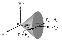
(b)

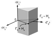
Abbildung 1: The Lie wedge for the system of Example 2 satisfying the (WH)-condition is four-dimensional: it contains (a) the convex cone $\mathfrak{c}_{0}$ (see (42) with $\lambda=1$) generated by $e^{\theta H_{y}}(\Gamma_{0}+H_{z})e^{-\theta H_{y}}$ and shown in the projection into the subspace spanned by $\{H_{x},H_{z},\Gamma_{0}\}$; and it comprises (b) the prism-shaped wedge projected into the subspace spanned by $\{H_{y},H_{z},\Gamma_{0}\}$. Note that the edge of the wedge is spanned by the control Hamiltonian $H_{y}$. Both parts of the figure scale with $\lambda\to\infty$.

Proposition III.2

The set $\mathfrak{w}_{0}=\mathbb{R}H_{y}\oplus(-\mathfrak{c}_{0})$ is the global Lie wedge to control system (36).

Proof:

The Lie wedge property of $\mathfrak{w}_{0}$ can be derived as in Example 1. Then the globality of $\mathfrak{w}_{0}$ follows again from Theorem 3. ∎

Remark 2

For clarity, let us denote the Lie wedge of Example 1 for $\Gamma_{0}$ as in (37) by $\mathfrak{w}^{\prime}_{0}$ while $\mathfrak{w}_{0}$ still refers to the Lie wedge of Example 2. Clearly, one has $\mathfrak{w}_{0}\subset\mathfrak{w}^{\prime}_{0}$ and $E(\mathfrak{w}_{0})=E(\mathfrak{w}^{\prime}_{0})\cap\mathfrak{w}_{0}$. Hence globality of $\mathfrak{w}_{0}$ also follows by Corollary II.2 and the globality of $\mathfrak{w}^{\prime}_{0}$.

Note that the Lie wedge $\mathfrak{w}_{0}$ in Example 2 does not specialise to the form of a Lie semialgebra as can readily be verified by a counter example: According to (42), choose $B\in\mathfrak{w}_{0}$ as $B=\Gamma_{0}+H_{x}$ (recalling $\Gamma_{0}:=E_{11}+E_{33}$ and $A=\Gamma_{0}+H_{z}$). Then by the commutator relations of Tab. I, the BCH product

$$A\star B=2\Gamma_{0}+H_{x}+H_{z}+\tfrac{1}{2}(H_{y}+p_{x}+p_{z})\,+\,\dots$$ (44)

immediately leads outside the Lie wedge $\mathfrak{w}_{0}$, e.g., by the non-vanishing component $p_{x}+p_{z}$. (NB: This argument can be made rigorous by introducing a scaling factor $t$ to give $tA\star tB$).

Finally, the edge of $\mathfrak{w}_{0}$ in Example 2 is $E(\mathfrak{w}_{0})=\mathbb{R}H_{y}$ (for $\gamma>0$, see Fig. 1) while in the limit of a closed system, i.e. for $\gamma=0$, it turns into the entire Lie algebra $\mathfrak{so}(3)$.

III-C Example 3: Corresponds to a Qubit System with Condition (WH) Satisfied and General Diagonal Relaxation Operator

Consider the contol system in $GL(3,\mathbb{R}^{\,}{})$ given by

$$\dot{X}=-(A+B_{u})X\;,$$ (45)

where $A:=\Gamma_{0}+H_{z}$, $B:=uH_{y}$, and

$$\Gamma_{0}:=\gamma\,\operatorname{diag}{}(1,1,2)$$ (46)

with $u\in\mathbb{R}$ and $\gamma\geq 0$. So for approximating the corresponding Lie wedge, we take the first step to be

$$\mathfrak{w}_{1}:=\mathbb{R}H_{y}\oplus(-\mathfrak{c}_{1})\;,$$ (47)

with $\mathfrak{c}_{1}:=\mathbb{R}_{0}^{+}(H_{z}+\Gamma_{0})$ and edge given by the span of $H_{y}$ — the control ‘Hamiltonian’. Again, in step (2) we identify the conjugation to be brought about by $\operatorname{Ad}_{\exp E(\mathfrak{w})}$ acting on the drift terms such as to give in step (3) the set

$$\mathfrak{c}_{3}=\mathbb{R}_{0}^{+}\{R_{y}(\theta)(\Gamma_{0}+H_{z})R_{y}(\theta)^{\top}\;|\;\theta\in\mathbb{R}\}$$ (48)

with the $\mathfrak{k}$-component brought about by the conjugated drift

$$R_{y}(\theta)H_{z}R_{y}(\theta)^{\top}=\cos(\theta)H_{z}+\sin(\theta)H_{x}$$ (49)

and the $\mathfrak{p}$-component reading

$$\begin{split}R_{y}&(\theta)\Gamma_{0}R_{y}(\theta)^{\top}\;=\;\gamma\left[\begin{smallmatrix}1+\sin^{2}(\theta)&&0&&\sin(\theta)\cos(\theta)\\ 0&&1&&0\\ \sin(\theta)\cos(\theta)&&0&&1+\cos^{2}(\theta)\end{smallmatrix}\right]\\[5.69054pt] &=\Gamma_{0}+\tfrac{\gamma}{2}\Delta_{13}-\tfrac{\gamma}{2}\big{(}\cos(2\theta)\Delta_{13}-\sin(2\theta)p_{y}\big{)}\\[5.69054pt] &=\tfrac{11+\cos(2\theta)}{12}\Gamma_{0}+\tfrac{\gamma}{2}\big{(}(1-\cos(2\theta))\Delta+\sin(2\theta)p_{y}\big{)}\;,\\ \end{split}$$ (50)

where the matrices $\Delta_{ij}$ and $p_{y}$ are defined as in Tab. I, and, for the sake of orthogonality, $\Delta:=\tfrac{2}{9}{\rm 1\negthickspace l}{}+\tfrac{1}{18}\Delta_{12}+\tfrac{8}{9}\Delta_{13}$.

Therefore, the Lie wedge can be expanded within the five-dimensional Hilbert space $\mathcal{H}:=\mbox{span}\{H_{x},H_{z},p_{y},\Delta,\Gamma_{0}\}$ and the final inner approximation to the Lie wedge takes the form

$$\mathfrak{w}_{0}:=\mathbb{R}H_{y}\oplus-\mathfrak{c}_{0}\;,$$ (51)

where $\mathfrak{c}_{0}$ is parameterised (again in the short-hand of (41)) as

$$\mathfrak{c}_{0}:=\mathbb{R}^{\,}{}_{0}^{+}\operatorname{conv}{}\Big{\{}\left[\begin{smallmatrix}2\sin(\theta)\\ 2\cos(\theta)\\ \gamma\sin(2\theta)\\ \gamma(1-\cos(2\theta))\\[1.42262pt] (11+\cos(2\theta))/6\end{smallmatrix}\right]\cdot\left[\begin{smallmatrix}H_{x}\\ H_{z}\\ p_{y}\\ \Delta\\[1.42262pt] \Gamma_{0}\end{smallmatrix}\right]\;\Big{|}\;\theta\in\mathbb{R}^{\,}{}\Big{\}}.$$ (52)

It is shown in Fig. 2. — As in Example 2, letting $\operatorname{Ad}_{\exp E(\mathfrak{w})}$ act on the drift terms adds no further elements to the edge of the wedge, so one gets:

Proposition III.3

The set $\mathfrak{w}_{0}=\mathbb{R}H_{y}\oplus(-\mathfrak{c}_{0})$ is the global Lie wedge to control system (45).

Proof:

The Lie wedge property of $\mathfrak{w}_{0}$ can be derived as in Example 1. Then the globality of $\mathfrak{w}_{0}$ follows again from Theorem 3. ∎

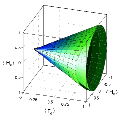
Abbildung 2: (Colour online) The Lie wedge of the more general system in Example 3 is five-dimensional. Here the surface of the convex cone $\mathfrak{c}_{0}$ generated by $e^{\theta H_{y}}(\Gamma_{0}+H_{z})e^{-\theta H_{y}}$ (see (52) with $\lambda=1$) is projected into the subspace $\mbox{span}\{H_{x},H_{z},\Gamma_{0}\}$. Since $[\Gamma_{0},H_{y}]\neq 0$ it deviates from the rotational symmetry of Example 2 given in the inner part for comparison, cp Fig. 1(a). The figure scales with $\lambda\to\infty$. The prism-shaped projection into the subspace $\mbox{span}\{H_{y},H_{z},\Gamma_{0}\}$ (not shown) is similar to that of Example 2 already given in Fig. 1(b).

Generalising the relaxation operator in Example 3 to $\Gamma_{0}:=\gamma\,\operatorname{diag}{}(a,b,c)$ with $a,b,c,\gamma\geq 0$ results in a generalised $\mathfrak{p}$-component replacing (50) by

$$\begin{split}&R_{y}(\theta)\Gamma_{0}R_{y}(\theta)^{\top}\;=\;\gamma\left[\begin{smallmatrix}a+(c-a)\sin^{2}(\theta)&&0&&(c-a)\sin(\theta)\cos(\theta)\\ 0&&b&&0\\ (c-a)\sin(\theta)\cos(\theta)&&0&&c-(c-a)\sin^{2}(\theta)\end{smallmatrix}\right]\\[5.69054pt] &=\Gamma_{0}+\gamma(c-a)\sin^{2}(\theta)\Delta_{13}+\gamma(c-a)\sin(\theta)\cos(\theta)p_{y}\\[5.69054pt] &=\Gamma_{0}+\tfrac{\gamma(c-a)}{2}\Delta_{13}-\tfrac{\gamma(c-a)}{2}\big{(}\cos(2\theta)\Delta_{13}-\sin(2\theta)p_{y}\big{)}\end{split}$$

This leads to a cone $\mathfrak{c}_{0}$ for (51) that keeps the structure of (52) in a slightly more general form, where Example 2 is readily reproduced by $c=a$, while Example 3 follows for $a=b=1$ and $c=2$.

The Lie wedge in Example 3 and its generalised form treated above do not take the form of a Lie semialgebra either. Choose $B:=H_{y}$ from the wedge $\mathfrak{w}_{0}$ of (51) and recall $A:=\Gamma_{0}+H_{z}$. Then the BCH product

$$A\star B=\Gamma_{0}+H_{y}+H_{z}-\tfrac{1}{2}(H_{x}+p_{y})\,+\,\dots$$ (53)

leads outside the Lie wedge of (51) since the component $H_{x}+p_{y}$ is not within the cone (52).

As pointed out already, in this section, we have chosen a representation in $\mathbb{R}^{3}$ in order to visualise the Hamiltonian parts of the respective quantum dynamics by $SO(3)$-rotations. In quantum mechanics, this picture can be recovered in the so-called coherence-vector representation [27]. Therefore, when taking an explicit spin-$\tfrac{1}{2}$ representation of $\operatorname{ad}_{\mathfrak{su}(2)}$ in the following chapter, the key results obtained here in Examples 1 through 3 will show up again.

IV Open Single-Qubit Quantum Systems

In this section, we analyze the standard single-qubit unital quantum systems beyond their purely dissipative evolution by allowing for Hamiltonian drifts and controls. In view of steering open quantum systems, this is an important generalisation.

IV-A Markovian Master Equation in Qubit Representation

Based on the Pauli matrices

$$\sigma_{x}:=\left[\begin{matrix}0&1\\ 1&0\end{matrix}\right],\quad\sigma_{y}:=\left[\begin{matrix}0&-i\\ i&0\end{matrix}\right],\quad\sigma_{z}:=\left[\begin{matrix}1&0\\ 0&-1\end{matrix}\right]$$ (54)

in this section we deliberately depart from the previous notation by using the explicit spin-$\tfrac{1}{2}$ adjoint representation carrying the spin-quantum number $j=\tfrac{1}{2}$ as prefactor in given by

$$\hat{\sigma}_{\nu}:=\tfrac{1}{2}({\rm 1\negthickspace l}{}_{2}\otimes\sigma_{\nu}-\sigma_{\nu}^{\top}\otimes{\rm 1\negthickspace l}{}_{2})\;,$$ (55)

for $\nu\in\{x,y,z\}$, where $\otimes$ denotes the Kronecker product of matrices. One easily recovers the $\mathfrak{su}(2)$ commutation relations

$$[i\,\hat{\sigma}_{p},i\,\hat{\sigma}_{q}]=-\varepsilon_{pqr}\;i\,\hat{\sigma}_{r}$$ (56)

to convince oneself of $\widehat{\operatorname{ad}}_{\mathfrak{su}(2)}:=\langle i\hat{\sigma}_{x},i\hat{\sigma}_{y},i\hat{\sigma}_{z}\rangle{}_{\sf Lie}\overset{\rm iso}{=}\operatorname{ad}_{\mathfrak{su}(2)}$. Here and henceforth we use $\varepsilon_{pqr}$ to discriminate even and odd permutations of $(x,y,z)$ by their signs, i.e. $\varepsilon_{pqr}=+1$ if $(p,q,r)$ is an even permutation of $(x,y,z)$, while $\varepsilon_{pqr}=-1$ for an odd permutation.

Thus for a single open qubit system in the above representation the controlled master equation (13) or rather its group lift (16) takes the explicit form

$$\dot{X}(t)=-\Big{(}i\big{(}\hat{H}_{d}+\sum_{j}u_{j}\hat{H}_{j}\big{)}+\hat{\Gamma}_{L}\Big{)}\,X(t)\,.$$ (57)

Here, $X(t)$ may be a density operator regarded (via the so-called $\operatorname{vec}{}$-representation or a qubit quantum channel represented in $GL(4,\mathbb{C})$. Moreover, $\hat{H}_{d}$ and $\hat{H}_{j}$ are in general of the from $\hat{H}_{d}:=({\rm 1\negthickspace l}{}_{2}\otimes H_{d}-H_{d}^{\top}\otimes{\rm 1\negthickspace l}{}_{2})$ and similar $\hat{H}_{j}$. To ensure complete positivity, the relaxation term $\hat{\Gamma}_{L}$ shall be again of Lindblad-Kossakowski form which for the standard unital single-qubit systems (with $V_{k}$ Hermitian) simply reads $\hat{\Gamma}_{L}=2\sum_{k}\gamma_{k}\;\hat{\sigma}_{k}^{2}$ to give the nicely structured generator

$$\mathcal{L}_{u}=i\big{(}\hat{H}_{d}+\sum_{j}u_{j}\hat{H}_{j}\big{)}+\;2\negthickspace\negthickspace\sum_{k\in\{x,y,z\}}\negthickspace\negthickspace\gamma_{k}\;\hat{\sigma}_{k}^{2}\;.$$ (58)

The generator is of this form because the $i\hat{H}$ terms are in the $\mathfrak{k}$-part of the Cartan decomposition of $\mathfrak{gl}(4,\mathbb{C})$ into skew-Hermitian ($\mathfrak{k}$) and Hermitian ($\mathfrak{p}$) matrices, whereas the $\hat{\sigma}_{k}^{2}$ terms are in the $\mathfrak{p}$-part.

IV-B Single-Qubit Systems Satisfying Condition (H)

Here we consider the class of fully Hamiltonian controllable unital single-qubit systems whose dissipation is governed by a single Lindblad operator $\hat{\sigma}_{k}^{2}$ for some $k\in\{x,y,z\}$ i.e. two of the three prefactors $\gamma_{x},\gamma_{y},\gamma_{z}$ have to vanish.

Similar to Example 1 of Sec. III, choose the controls $\hat{\sigma}_{x}$ and $\hat{\sigma}_{y}$ to see that such a system fulfills condition (H), since $\langle i\hat{\sigma}_{x},i\hat{\sigma}_{y}\rangle{}_{\sf Lie}=\widehat{\operatorname{ad}}_{\mathfrak{su}(2)}$. Then it is actually immaterial which single Pauli matrix is chosen as the Lindblad operator $\hat{\sigma}^{2}_{k}$, because all of the Pauli matrices are unitarily equivalent. So without loss of generality, one may choose $k=z$, i.e. $\gamma_{x}=0$, $\gamma_{y}=0$, and $\gamma_{z}=:\gamma$.

Therefore the fully Hamiltonian controllable version of the bit-flip, phase-flip, and bit-phase-flip channels are dynamically equivalent in as much as they have (up to unitary equivalence) a common global Lie wedge

$$\mathfrak{w}_{0}:=\widehat{\operatorname{ad}}_{\mathfrak{su}(2)}\oplus-\mathfrak{c}_{0}\;,$$ (59)

where the cone $\mathfrak{c}_{0}$ is defined by

$$\mathfrak{c}_{0}:=\mathbb{R}^{\,}{}_{0}^{+}\mbox{conv}\left\{\hat{U}\,\hat{\sigma}_{z}^{2}\,\hat{U}^{\dagger}\;\big{|}\;U\in SU(2)\right\}\\ \quad$$ (60)

with

$$\hat{U}:=\bar{U}\otimes U\;.$$ (61)

Clearly, the wedge $\mathfrak{w}_{0}$ is global by Corollary II.1 or, alternatively, by Theorem 3 and its edge $E(\mathfrak{w}_{0})$ is given by the Lie subalgebra $\widehat{\operatorname{ad}}_{\mathfrak{su}(2)}$. The above Lie wedge is isomorphic to the one in Example 1 of Sec. III for the particular choice that $\Gamma_{0}=\operatorname{diag}{}(1,1,0)$.

IV-C Single-Qubit Systems Satisfying Condition (WH): One Lindblad Operator

Here we discuss an important class of standard single-qubit systems which are particularly simple in three regards

1. their dissipative term is governed by a single Lindblad operator, $\Gamma_{0}:=2\gamma\hat{\sigma}^{2}_{k}$ for some $k\in\{x,y,z\}$;

2. their switchable Hamiltonian control is brought about by a single Hamiltonian $\hat{\sigma}_{c}$ for some $c\in\{x,y,z\}$;

3. their non-switchable Hamiltonian drift is $\hat{\sigma}_{d}$ for some $d\in\{x,y,z\}$.

Applying the algorithm for the inner approximation of the Lie wedge, we get in step (1)

$$\mathfrak{w}^{c}_{dk}(1):=i\;\mathbb{R}\hat{\sigma}_{c}\oplus\,-\mathbb{R}_{0}^{+}\big{(}i\hat{\sigma}_{d}+2\gamma\hat{\sigma}_{k}^{2}\big{)}\;,$$ (62)

where again we note the separation by $\mathfrak{k}$-$\mathfrak{p}$ components. In step (2) we identify the span generated by the control $i\hat{\sigma}_{c}$ as the edge $E(\mathfrak{w})$ of the wedge. So the conjugation has to be by the control subgroup, i.e. by $e^{-i2\theta\hat{\sigma}_{c}}=e^{+i\theta\sigma_{c}^{\top}}\otimes e^{-i\theta\sigma_{c}}$. Thus in step (3) one obtains as $\mathfrak{k}$-component of the conjugated drift

$$\begin{split}K_{d}^{c}(\theta):=&\quad e^{-i\theta\hat{\sigma}_{c}}(i\hat{\sigma}_{d})e^{i\theta\hat{\sigma}_{c}}\\ =&\begin{cases}i\,\hat{\sigma}_{d}&\text{for $c=d$}\\ i\,\cos(\theta)\hat{\sigma}_{d}+i\,\varepsilon_{cdq}\sin(\theta)\hat{\sigma}_{q}&\text{else}\end{cases}\end{split}$$ (63)

and as $\mathfrak{p}$-component

$$\begin{split}P_{k}^{c}(\theta):=&\quad e^{-i\theta\hat{\sigma}_{c}}(2\gamma\,\hat{\sigma}_{k}^{2})e^{i\theta\hat{\sigma}_{c}}\\[2.84526pt] =&\begin{cases}2\gamma\,\hat{\sigma}_{k}^{2}&\text{for $c=k$}\\[2.84526pt] 2\gamma\,\big{(}\cos(\theta)\hat{\sigma}_{k}+\,\varepsilon_{ckr}\sin(\theta)\hat{\sigma}_{r}\big{)}^{2}&\text{else}\;.\end{cases}\end{split}$$ (64)

The last expression (for $c\neq k$) can be further resolved using the anticommutator $\left\{A,B\right\}_{+}:=AB+BA$

$$\begin{split}P^{c}_{k}(\theta)&=2\gamma\left[\begin{smallmatrix}\cos^{2}(\theta)\\ \sin^{2}(\theta)\\ \cos(\theta)\sin(\theta)\end{smallmatrix}\right]\cdot\left[\begin{smallmatrix}\hat{\sigma}_{k}^{2}\\ \hat{\sigma}_{r}^{2}\\ \varepsilon_{ckr}\{\hat{\sigma}_{k},\hat{\sigma}_{r}\}_{+}\end{smallmatrix}\right]\,.\\[5.69054pt] &=\tfrac{\gamma}{2}\left[\begin{smallmatrix}2\\ 1+\cos(2\theta)\\ 1-\cos(2\theta)\\ \sin(2\theta)\end{smallmatrix}\right]\cdot\left[\begin{smallmatrix}{\rm 1\negthickspace l}{}\\ -(\sigma^{\top}_{k}\otimes\sigma_{k})\\ -(\sigma^{\top}_{r}\otimes\sigma_{r})\\ -\varepsilon_{ckr}((\sigma^{\top}_{k}\otimes\sigma_{r})+(\sigma^{\top}_{r}\otimes\sigma_{k}))\end{smallmatrix}\right]\;,\\ \end{split}$$ (65)

where the latter identity gives a decomposition into mutually orthogonal Pauli-basis elements.

To summarize, if the control Hamiltonian neither commutes with the Hamiltonian part nor with the dissipative part of the drift, one obtains in terms of the above $K_{d}^{c}(\theta)$ and $P_{k}^{c}(\theta)$

$$\mathfrak{c}_{dk}^{c}:=\mathbb{R}_{0}^{+}\operatorname{conv}{}\{K_{d}^{c}(\theta)+P_{k}^{c}(\theta)\,|\,\theta\in\mathbb{R}^{\,}{}\,\}$$ (66)

However, if $[\hat{\sigma}_{c},\Gamma_{0}]=0$, then the convex cone in equation (66) simplifies by $P_{k}^{c}(\theta)=\Gamma_{0}$ to

$$\mathfrak{c}_{dk}^{c}=\mathbb{R}^{\,}{}_{0}^{+}\operatorname{conv}{}\Big{\{}\left[\begin{smallmatrix}\cos(\theta)\\ \sin(\theta)\\ 1\end{smallmatrix}\right]\cdot\left[\begin{smallmatrix}i\hat{\sigma}_{d}\\ i\varepsilon_{cdq}\hat{\sigma}_{q}\\ \Gamma_{0}\end{smallmatrix}\right]\;\Big{|}\;\theta\in\mathbb{R}^{\,}{}\Big{\}}\quad$$ (67)

in entire analogy to Example 2 of Sec. III.

The final Lie wedge admits the orthogonal decomposition

$$\mathfrak{w}^{c}_{dk}:=i\mathbb{R}\,\hat{\sigma}_{c}\oplus-\mathfrak{c}^{c}_{dk}$$ (68)

and moreover by Theorem 3 (or alternatively by Corollary II.2) it is global. For $\gamma>0$, the edge $E(\mathfrak{w})=\langle i\,\hat{\sigma}_{c}\rangle{}$ is again the span generated by the control, yet it flips into the full algebra $E(\mathfrak{w})=\widehat{\operatorname{ad}}_{\mathfrak{su}(2)}$ in the limit $\gamma=0$.

The relation to Examples 2 and 3 of Sec. III is obvious: Let a unital qubit system satisfy the (WH)-condition and have a dissipative Lindbladian $\Gamma_{0}:=2\gamma\hat{\sigma}_{k}^{2}$ induced by a single Lindblad operator $V_{k}=\sigma_{k}$. If $[\hat{\sigma}_{c},\Gamma_{0}]\neq 0$, one arrives at a situation resembling Example 3, whereas if $[\hat{\sigma}_{c},\Gamma_{0}]=0$, one obtains a result analogous to Example 2.

Application: Bit-Flip and Phase-Flip Channels

Also the relation to standard unital qubit channels is immediate: Note that in the bit-flip channel the noise is generated by $\hat{\sigma}_{x}^{2}$, while it is $\hat{\sigma}_{y}^{2}$ in the bit-phase-flip channel and $\hat{\sigma}_{z}^{2}$ in the phase-flip channel, see Tab. II. In the absence of any coherent drift or control brought about by the respective Hamiltonians $H_{d}=\hat{\sigma}_{d}$ or $H_{j}=\hat{\sigma}_{j}$, the Kraus representations are standard. By allowing for drifts and controls, the Kraus rank $K$ of the channel usually increases to $K$=$4$ with exception of a single $\hat{\sigma}_{d}$ or $\hat{\sigma}_{j}$ commuting with the single Lindblad operator $\hat{\sigma}_{k}^{2}$ keeping $K$=$2$. Also the time dependences become more involved. Hence explicit results will be given elsewhere.

Under full H-controllability, the Lie wedges of all the three channels become equivalent as the Pauli matrices and thus the corresponding noise generators are unitarily similar.

In contrast, for the case satisfying the (WH)-condition, assume a control system with a Hamiltonian drift term governed by $\hat{\sigma}_{z}$. Upon including relaxation, now there are two different scenarios: if the control Hamiltonian (indexed by $c\in\{x,y,z\}$) commutes with the noise generator (indexed by $k\in\{x,y,z\}$), one finds a situation as in Example 2 and (67), otherwise the scenario is more general as in (66).

Tabelle II: Controlled Single-Qubit Channels and Their Lie Wedges

Channel	Primary∗ Lindblad Operators	Primary∗ Kraus Operators	———————— Lie Wedges ————————- XXXX
			case satisfying (WH)-condition	H-controllable case
Bit Flip	$V_{1}=\sqrt{a_{11}}\;\sigma_{x}$	$E_{1}=\sqrt{r_{11}}\;\sigma_{x}$	$\mathfrak{w}_{dx}^{c}=\langle i\hat{\sigma}_{c}\rangle\oplus-\mathfrak{c}_{dx}^{c}$	$\mathfrak{w}=\widehat{\operatorname{ad}}_{\mathfrak{su}(2)}\oplus-\mathfrak{c}_{0}$
		$E_{0}=\sqrt{q_{11}}\;{\rm 1\negthickspace l}{}$	[see Eqns. (66,67)]	[see Eqn. (60)]
Phase Flip	$V_{1}=\sqrt{a_{22}}\;\sigma_{z}$	$E_{1}=\sqrt{r_{22}}\;\sigma_{z}$	$\mathfrak{w}_{dz}^{c}=\langle i\hat{\sigma}_{c}\rangle\oplus-\mathfrak{c}_{dz}^{c}$	—same as above—
		$E_{0}=\sqrt{q_{22}}\;{\rm 1\negthickspace l}{}$	[see Eqns. (66,67)]
Bit-Phase Flip	$V_{1}=\sqrt{a_{33}}\;\sigma_{y}$	$E_{1}=\sqrt{r_{33}}\;\sigma_{y}$	$\mathfrak{w}_{dy}^{c}=\langle i\hat{\sigma}_{c}\rangle\oplus-\mathfrak{c}_{dy}^{c}$	—same as above—
		$E_{0}=\sqrt{q_{33}}\;{\rm 1\negthickspace l}{}$	[see Eqns. (66,67)]
Depolarizing	$V_{1}=\sqrt{a_{11}}\;\sigma_{x}$	$E_{1}=\sqrt{r_{1}}\;\sigma_{x}$	$\mathfrak{w}_{d,xyz}^{c}=\langle i\hat{\sigma}_{c}\rangle\oplus-\mathfrak{c}_{d,xyz}^{c}$	$\mathfrak{w}=\widehat{\operatorname{ad}}_{\mathfrak{su}(2)}\oplus-\mathfrak{c}_{xyz}$
	$V_{2}=\sqrt{a_{22}}\;\sigma_{y}$	$E_{2}=\sqrt{r_{2}}\;\sigma_{y}$	[see Eqn. (63) and Eqns. (70,71)]	[see Eqns. (72,73)]
	$V_{3}=\sqrt{a_{33}}\;\sigma_{z}$	$E_{3}=\sqrt{r_{3}}\;\sigma_{z}$
		$E_{0}=\sqrt{r_{0}}\;{\rm 1\negthickspace l}{}$
∗) Primary operators are for purely dissipative time evolutions (no Hamiltonian drift no control). Then the time dependence of the
Kraus operators roots in the GKS matrix $\{a_{ii}\}_{i=1}^{3}$. Define: $\lambda_{1}:=a_{22}+a_{33},\lambda_{2}:=a_{22}-a_{33},\lambda_{3}:=a_{11}+a_{22}$, and thereby $q_{ii}:=\tfrac{1}{2}(1+e^{-a_{ii}t}),$
$r_{ii}:=\tfrac{1}{2}(1-e^{-a_{ii}t})$ and $r_{0}:=\tfrac{1}{4}(1+e^{-\lambda_{1}t}+e^{-\lambda_{2}t}+e^{-\lambda_{3}t}),\;r_{1}:=\tfrac{1}{4}(1-e^{-\lambda_{1}t}+e^{-\lambda_{2}t}-e^{-\lambda_{3}t}),\;r_{2}:=\tfrac{1}{4}(1+e^{-\lambda_{1}t}-e^{-\lambda_{2}t}-e^{-\lambda_{3}t})$,
$r_{3}:=\tfrac{1}{4}(1-e^{-\lambda_{1}t}-e^{-\lambda_{2}t}+e^{-\lambda_{3}t})$. — Under Hamiltonian drift and control the Kraus-rank gets $K=4$ except for one single control $H_{c}$ or drift $H_{d}$
that commutes with the only Lindblad operator $V_{k}$: in this case the Kraus rank is $K=2$. Time-dependences are involved and will be given elsewhere.
The Pauli matrices $\sigma_{\nu}$ are defined in Eqn. (54).

IV-D Single-Qubit Systems Satisfying Condition (WH): Several Lindblad Operators

Consider a unital qubit system satisfying the (WH)-condition and whose Lindbladian $\Gamma_{0}$ is generated by $\ell=2$ or $\ell=3$ different Lindblad operators $\hat{\sigma}_{k}^{2}$. Then one obtains the following generalisations of the symmetric component $P_{k}^{c}(\theta)\in\mathfrak{c}_{dk}^{c}$.
For $\ell=2$ and $\sigma_{c}\perp\sigma_{k}$, $\sigma_{c}=\sigma_{k^{\prime}}$

$$\begin{split}P^{c}_{kk^{\prime}}(\theta)&=2\left[\begin{smallmatrix}\gamma^{\prime}\\ \gamma\cos^{2}(\theta)\\ \gamma\sin^{2}(\theta)\\ \gamma\cos(\theta)\sin(\theta)\end{smallmatrix}\right]\cdot\left[\begin{smallmatrix}\hat{\sigma}^{2}_{k^{\prime}}\\ \hat{\sigma}^{2}_{k}\\ \hat{\sigma}_{r}^{2}\\ \varepsilon_{ckr}\{\hat{\sigma}_{k},\hat{\sigma}_{r}\}_{+}\end{smallmatrix}\right]\\[5.69054pt] =\tfrac{1}{2}&\left[\begin{smallmatrix}\gamma^{\prime}\\ 2(\gamma+\gamma^{\prime})\\ \gamma(1+\cos(2\theta))\\ \gamma(1-\cos(2\theta))\\ \gamma\sin(2\theta)\end{smallmatrix}\right]\cdot\left[\begin{smallmatrix}-(\sigma^{\top}_{k^{\prime}}\otimes\sigma_{k^{\prime}})\\ {\rm 1\negthickspace l}{}\\ -(\sigma^{\top}_{k}\otimes\sigma_{k})\\ -(\sigma^{\top}_{r}\otimes\sigma_{r})\\ -\varepsilon_{ckr}((\sigma^{\top}_{r}\otimes\sigma_{k})+(\sigma^{\top}_{k}\otimes\sigma_{r}))\end{smallmatrix}\right].\\[5.69054pt] \end{split}$$ (69)

while for $\ell=3$ and $\sigma_{c}\perp\sigma_{k}$, $\sigma_{c}\perp\sigma_{k^{\prime}}$, $\sigma_{c}=\sigma_{k^{\prime\prime}}$

$$\begin{split}&P^{c}_{kk^{\prime}k^{\prime\prime}}(\theta)=2\left[\begin{smallmatrix}\gamma^{\prime\prime}\\ \gamma\cos^{2}(\theta)+\gamma^{\prime}\sin^{2}(\theta)\\ \gamma^{\prime}\cos^{2}(\theta)+\gamma\sin^{2}(\theta)\\ (\gamma-\gamma^{\prime})\cos(\theta)\sin(\theta)\end{smallmatrix}\right]\cdot\left[\begin{smallmatrix}\hat{\sigma}^{2}_{k^{\prime\prime}}\\ \hat{\sigma}^{2}_{k}\\ \hat{\sigma}^{2}_{k^{\prime}}\\ \varepsilon_{ckk^{\prime}}\{\hat{\sigma}_{k},\hat{\sigma}_{k^{\prime}}\}_{+}\end{smallmatrix}\right]\\[5.69054pt] =\tfrac{1}{2}&\left[\begin{smallmatrix}\gamma^{\prime\prime}\\ 2(\gamma+\gamma^{\prime}+\gamma^{\prime\prime})\\ \gamma+\gamma^{\prime}+(\gamma-\gamma^{\prime})\cos(2\theta)\\ \gamma+\gamma^{\prime}-(\gamma-\gamma^{\prime})\cos(2\theta)\\ (\gamma-\gamma^{\prime})\sin(2\theta)\end{smallmatrix}\right]\cdot\left[\begin{smallmatrix}-(\sigma^{\top}_{k^{\prime\prime}}\otimes\sigma_{k^{\prime\prime}})\\ {\rm 1\negthickspace l}{}\\ -(\sigma^{\top}_{k}\otimes\sigma_{k})\\ -(\sigma^{\top}_{k^{\prime}}\otimes\sigma_{k^{\prime}})\\ -\varepsilon_{ckk^{\prime}}((\sigma^{\top}_{k^{\prime}}\otimes\sigma_{k})+(\sigma^{\top}_{k}\otimes\sigma_{k^{\prime}}))\end{smallmatrix}\right].\\[5.69054pt] \end{split}$$ (70)

which for $\gamma=\gamma^{\prime}=\gamma^{\prime\prime}$ simplifies to

$$P^{c}_{kk^{\prime}k^{\prime\prime}}(\theta)=\Gamma_{0}=2\gamma(\hat{\sigma}^{2}_{k}+\hat{\sigma}^{2}_{k^{\prime}}+\hat{\sigma}^{2}_{k^{\prime\prime}})\;.$$ (71)

Note that (69) with $\gamma=\gamma^{\prime}$ precisely corresponds to Example 3 in Sec. III.

Application: Depolarising Channel

Treating the depolarising channel also becomes immediate, since one has three noise generators governed by all of $\hat{\sigma}_{x},\hat{\sigma}_{y}$, and $\hat{\sigma}_{z}$. Thus the fully Hamiltonian controllable version of the depolarising channel follows the bit-flip and phase-flip channels in the structure of its global Lie wedge

$$\mathfrak{w}_{0}:=\widehat{\operatorname{ad}}_{\mathfrak{su}(2)}\oplus-\mathfrak{c}_{xyz}\;,$$ (72)

where the cone $\mathfrak{c}_{xyz}$ now reads

$$\mathfrak{c}_{xyz}:=\mathbb{R}^{\,}{}_{0}^{+}\mbox{conv}\big{\{}\hat{U}(\gamma_{x}\hat{\sigma}_{x}^{2}+\gamma_{y}\hat{\sigma}_{y}^{2}+\gamma_{z}\hat{\sigma}_{z}^{2})\hat{U}^{\dagger}\;|\;U\in SU(2)\big{\}}$$ (73)

with $\hat{U}$ of the form (61). Again, the edge of the wedge is given by the entire algebra $E(\mathfrak{w})=\widehat{\operatorname{ad}}_{\mathfrak{su}(2)}$ and globality of the wedge follows by Theorem 3 or Corollary II.1. — Moreover, note that the Lie wedge in the fully Hamiltonian controllable depolarising channel with isotropic noise takes the structure of a Lie semialgebra as (in the coherence-vector representation) it corresponds to the special case of Example 1 in Sec. III, where the relaxation operator is a scalar multiple of the unity, $\Gamma_{0}=\lambda\cdot{\rm 1\negthickspace l}{}$. For anisotropic relaxation, however, this feature does not arise.

If only condition (WH) is satisfied, there are two distinctions: if the noise contributions are isotropic (i.e. with equal contribution by all the Paulis through $\gamma_{x}=\gamma_{y}=\gamma_{z}$), one finds a cone expressed by (63) and (71). However, in the generic anisotropic case, the cone can be expressed by (63) and (70), see also Tab. II.

V Open Two-Qubit Quantum Systems

In this section we extend the notions introduced in the previous chapter to three types of two-qubit quantum systems with uncorrelated noise. The two qubits will be denoted $\sf{A}$ and $\sf{B}$, respectively. Moreover, we use the short-hands $\sigma_{\mu\nu}:=\sigma_{\mu}\otimes\sigma_{\nu}$ with $\mu,\nu\in\{x,y,z,1\}$, where $\sigma_{1}:={\rm 1\negthickspace l}{}$ as well as the corresponding ‘commutator superoperators’ $\hat{\sigma}_{\mu\nu}:=\tfrac{1}{2}({\rm 1\negthickspace l}{}\otimes\sigma_{\mu\nu}-\sigma_{\mu\nu}^{t}\otimes{\rm 1\negthickspace l}{})$.

V-A Fully H-Controllable Two-Qubit Channels

A fully Hamiltonian controllable two-qubit toy-model system with switchable Ising-coupling is given by the master equation

$$\dot{\rho}=-\big{(}i\sum_{j}u_{j}\hat{\sigma}_{j}+\Gamma_{0}\big{)}\rho\;$$ (74)

where $\hat{\sigma}_{j}\in\{\hat{\sigma}_{x1},\hat{\sigma}_{y1};\hat{\sigma}_{1x},\hat{\sigma}_{1y};\hat{\sigma}_{zz}\}$ are the Hamiltonian control terms with amplitudes $\left\{u_{j}\right\}_{j=1}^{5}\in\mathbb{R}$.

Since $\langle i\hat{\sigma}_{j}\,|\,j=1,2,\dots,5\rangle{}_{\sf Lie}=\widehat{\operatorname{ad}}_{\mathfrak{su}(4)}$, the edge of the wedge is $E(\mathfrak{w})=\widehat{\operatorname{ad}}_{\mathfrak{su}(4)}$. Following the algorithm for an inner approximation of the Lie wedge, step (1) thus gives

$$\mathfrak{w}_{1}:=\widehat{\operatorname{ad}}_{\mathfrak{su}(4)}\oplus-\mathbb{R}^{+}_{0}\Gamma_{0}\;.$$ (75)

Conjugating the dissipative component by the exponential map of the edge and then taking the convex hull yields the convex cone

$$\mathfrak{c}_{0}:=\mbox{conv}\big{\{}\lambda\hat{U}\Gamma_{0}\hat{U}^{\dagger}|\hat{U}:=\bar{U}\otimes U,U\in SU(4),\lambda\geq 0\big{\}}\;,$$ (76)

which is the two-qubit analogue of the cone in Eqn. (60). The resulting Lie wedge

$$\mathfrak{w}_{0}:=\widehat{\operatorname{ad}}_{\mathfrak{su}(4)}\oplus-\mathfrak{c}_{0}$$ (77)

is global by Theorem 3.

V-B Two-Qubit Channels Satisfying the (H)-Condition Locally and the (WH)-Condition Globally

By shifting the Ising coupling term from the set of switchable control Hamiltonians into the (non-switchable) drift term, $\hat{\sigma}_{d}=\hat{\sigma}_{zz}$, one obtains the realistic and actually widely occuring type of system

$$\dot{\rho}=-\big{(}i\hat{\sigma}_{d}+i\sum_{j}u_{j}\hat{\sigma}_{j}+\Gamma_{0}\big{)}\rho\;$$ (78)

where now one just has the local control terms $\hat{\sigma}_{j}\in\{\hat{\sigma}_{x1},\hat{\sigma}_{y1};\hat{\sigma}_{1x},\hat{\sigma}_{1y}\}$. Since $\langle i\hat{\sigma}_{x1},i\hat{\sigma}_{y1}\rangle{}_{\sf Lie}=\widehat{\operatorname{ad}}_{\mathfrak{su}_{\sf{A}}(2)}\otimes{\rm 1\negthickspace l}{}_{\sf{B}}$, whereas on the other hand $\langle i\hat{\sigma}_{1x},i\hat{\sigma}_{1y}\rangle{}_{\sf Lie}={\rm 1\negthickspace l}{}_{\sf{A}}\otimes\widehat{\operatorname{ad}}_{\mathfrak{su}_{\sf{B}}(2)}$, the edge of the wedge

$$E(\mathfrak{w})=\widehat{\operatorname{ad}}_{\mathfrak{su}_{\sf{A}}(2)\widehat{\oplus}\mathfrak{su}_{\sf{B}}(2)}$$ (79)

is in fact brought about by the Kronecker sum of local algebras

$$\mathfrak{su}_{\sf{A}}(2)\otimes{\rm 1\negthickspace l}{}_{\sf{B}}+{\rm 1\negthickspace l}{}_{\sf{A}}\otimes\mathfrak{su}_{\sf{B}}(2)=:\mathfrak{su}_{\sf{A}}(2)\widehat{\oplus}\mathfrak{su}_{\sf{B}}(2)$$ (80)

forming the generator of the group of local unitary actions

$$\exp\big{(}\mathfrak{su}_{\sf{A}}(2)\widehat{\oplus}\mathfrak{su}_{\sf{B}}(2)\big{)}=SU_{\sf{A}}(2)\otimes SU_{\sf{B}}(2)\;.$$ (81)

Remarkably, in this important class of open quantum-dynamical systems, qubits $\sf{A}$ and $\sf{B}$ are locally (H)-controllable, respectively, while globally the system satisfies but the (WH)-condition.

The final Lie wedge in these systems reads as

$$\mathfrak{w}_{dk}^{2\oplus 2}=\widehat{\operatorname{ad}}_{\mathfrak{su}_{\sf{A}}(2)\widehat{\oplus}\mathfrak{su}_{\sf{B}}(2)}\oplus-\mathfrak{c}_{dk}^{2\oplus 2}$$ (82)

with the convex cone

$$\mathfrak{c}_{dk}^{2\oplus 2}:=\mathbb{R}^{+}_{0}\operatorname{conv}{}\big{\{}K_{d}^{2\oplus 2}+P_{k}^{2\oplus 2}\big{\}}$$ (83)

being given in terms of the respective $\mathfrak{k}$ and $\mathfrak{p}$-components. Here we use the short-hand of (61) in the sense of $\hat{U}_{2\otimes 2}:=\bar{U}_{2\otimes 2}\otimes U_{2\otimes 2}$ to arrive at

$$K_{d}^{2\oplus 2} := \{\hat{U}_{2\otimes 2}(i\hat{\sigma}_{d})\hat{U}^{\dagger}_{2\otimes 2}\,|\,U_{2\otimes 2}\in SU(2)\otimes SU(2)\}\qquad$$ (84)

$$P_{k}^{2\oplus 2} := \{\hat{U}_{2\otimes 2}(\Gamma_{0})\hat{U}^{\dagger}_{2\otimes 2}\,|\,U_{2\otimes 2}\in SU(2)\otimes SU(2)\}\,.$$ (85)

As before, this immediately results from the initial wedge approximation by step (1)

$$\mathfrak{w}_{1}^{2\oplus 2}:=\widehat{\operatorname{ad}}_{\mathfrak{su}_{\sf{A}}(2)\widehat{\oplus}\mathfrak{su}_{\sf{B}}(2)}\oplus-\mathbb{R}^{+}_{0}(i\hat{\sigma}_{d}+\Gamma_{0})$$ (86)

followed by conjugation with $\operatorname{Ad}_{\exp E(\mathfrak{w})}=\operatorname{Ad}_{2\otimes 2}$ to give

$$K_{d}^{2\oplus 2}+P_{k}^{2\oplus 2}:=\mathcal{O}_{SU(2)\otimes SU(2)}\big{(}i\hat{\sigma}_{d}+\Gamma_{0}\big{)}\;.\quad$$ (87)

Step (3) then takes the convex hull. — To show globality, let $\mathfrak{w}^{\prime}$ denote the global Lie wedge corresponding to the fully H-controllable system given in Eqn.  (74). Then $\mathfrak{w}_{dk}^{2\oplus 2}\subset\mathfrak{w}^{\prime}$, and it can be shown that $\mathfrak{w}_{dk}^{2\oplus 2}$ satisfies the conditions of Corollary II.2 and therefore is global.

V-C Two-Qubit Channels Satisfying Only the (WH)-Condition

In the final example of a two-qubit system, the independent local controls shall even be limited to either $x$ or $y$-controls on the two qubits according to

$$\dot{\rho}=-\big{(}i(\hat{\sigma}_{d}+u_{\sf{A}}\hat{\sigma}_{c1}+u_{\sf{B}}\hat{\sigma}_{1c^{\prime}})+\Gamma_{0}\big{)}\rho\;,$$ (88)

where now $\hat{\sigma}_{d}:=i\big{(}\hat{\sigma}_{z1}+\hat{\sigma}_{1z}+\hat{\sigma}_{zz}\big{)}$ and $\hat{\sigma}_{c1}$ with a single $c\in\{x,y\}$ and likewise $\hat{\sigma}_{1c^{\prime}}$ with a single $c^{\prime}\in\{x,y\}$ and $u_{\sf{A}},u_{\sf{B}}\in\mathbb{R}$. Furthermore, assume the system undergoes local uncorrelated noise in each of the two subsystems in the sense that the Lindblad operators are of local form

$$V_{k} \in \{\sigma_{k1}\;|\;k\in\{x,y,z\}\}$$ (89)

$$V_{k^{\prime}} \in \{\hat{\sigma}_{1k^{\prime}}\;|\;k^{\prime}\in\{x,y,z\}\}\;,$$ (90)

where $k$ and $k^{\prime}$ are chosen independently $k,k^{\prime}\in\{x,y,z\}$ so that in the convention of (55) one finds

$$\Gamma_{0}\;:=\;2\gamma\hat{\sigma}_{k1}^{2}\;+\;2\gamma^{\prime}\hat{\sigma}^{2}_{1k^{\prime}}\;.$$ (91)

This system satisfies but the (WH)-condition both locally and globally, the latter following from

$$\langle i\hat{\sigma}_{c1},i\hat{\sigma}_{1c^{\prime}},i\hat{\sigma}_{d}\rangle{}_{\sf Lie}=\widehat{\operatorname{ad}}_{\mathfrak{su}(4)}\;.$$ (92)

The Lie wedge is given by

$$\mathfrak{w}^{cc^{\prime}}_{kk^{\prime}}:=\langle i\hat{\sigma}_{c}\rangle{}+\langle i\hat{\sigma}_{c^{\prime}}\rangle{}\oplus-\mathfrak{c}^{cc^{\prime}}_{kk^{\prime}}\;,$$ (93)

where the two-dimensional edge of the wedge is generated by the rays $\langle i\hat{\sigma}_{c1}\rangle{}$, $\langle i\hat{\sigma}_{1c^{\prime}}\rangle{}$ and the cone

$$\begin{split}\mathfrak{c}^{cc^{\prime}}_{kk^{\prime}}:=\mathbb{R}_{0}^{+}\operatorname{conv}{}\big{\{}&K^{c}(\theta)+K^{c^{\prime}}(\theta^{\prime})+K^{cc^{\prime}}(\theta,\theta^{\prime})\\ &+P_{k}^{c}(\theta)+P^{c^{\prime}}_{k^{\prime}}(\theta^{\prime})\,|\,\theta,\theta^{\prime}\in\mathbb{R}\,\big{\}}\end{split}$$ (94)

is given in terms of the $\mathfrak{k}$- and $\mathfrak{p}$-components (setting $\theta:=u_{\sf{A}}$ and $\theta^{\prime}:=u_{\sf{B}}$ and using the relations in (63)) as

$$K^{c}(\theta)+K^{c^{\prime}}(\theta^{\prime})+K^{cc^{\prime}}(\theta,\theta^{\prime})=\left[\begin{smallmatrix}\cos(\theta)\\ \sin(\theta)\\ \cos(\theta^{\prime})\\ \sin(\theta^{\prime})\\ \cos(\theta)\cos(\theta^{\prime})\\ \cos(\theta)\sin(\theta^{\prime})\\ \cos(\theta^{\prime})\sin(\theta)\\ \sin(\theta)\sin(\theta^{\prime})\end{smallmatrix}\right]\cdot i\left[\begin{smallmatrix}\hat{\sigma}_{z1}\\ \varepsilon_{czq}\hat{\sigma}_{q1}\\ \hat{\sigma}_{1z}\\ \varepsilon_{c^{\prime}zq^{\prime}}\hat{\sigma}_{1q^{\prime}}\\ \hat{\sigma}_{zz}\\ \varepsilon_{c^{\prime}zq^{\prime}}\hat{\sigma}_{zq^{\prime}}\\ \varepsilon_{czq}\hat{\sigma}_{qz}\\ \hat{\sigma}_{qq^{\prime}}\end{smallmatrix}\right]\qquad$$ (95)

and (as in (65))

$$\begin{split}P^{c}_{k}&(\theta)=2\gamma\left[\begin{smallmatrix}\cos^{2}(\theta)\\ \sin^{2}(\theta)\\ \cos(\theta)\sin(\theta)\end{smallmatrix}\right]\cdot\left[\begin{smallmatrix}\hat{\sigma}^{2}_{k1}\\ \hat{\sigma}^{2}_{r1}\\ \varepsilon_{ckr}\{\hat{\sigma}_{k1},\hat{\sigma}_{r1}\}_{+}\end{smallmatrix}\right]\\[5.69054pt] &=\tfrac{\gamma}{2}\left[\begin{smallmatrix}2\\ 1+\cos(2\theta)\\ 1-\cos(2\theta)\\ \sin(2\theta)\end{smallmatrix}\right]\cdot\left[\begin{smallmatrix}{\rm 1\negthickspace l}{}\\ -(\sigma^{\top}_{k}\otimes\sigma_{k})\otimes{\rm 1\negthickspace l}{}_{\sf{B}}\\ -(\sigma^{\top}_{r}\otimes\sigma_{r})\otimes{\rm 1\negthickspace l}{}_{\sf{B}}\\ -\varepsilon_{ckr}((\sigma^{\top}_{k}\otimes\sigma_{r})+(\sigma^{\top}_{r}\otimes\sigma_{k}))\otimes{\rm 1\negthickspace l}{}_{\sf{B}}\end{smallmatrix}\right]\\[5.69054pt] \end{split}$$ (96)

as well as

$$\begin{split}P^{c^{\prime}}_{k^{\prime}}&(\theta^{\prime})=2\gamma^{\prime}\left[\begin{smallmatrix}\cos^{2}(\theta^{\prime})\\ \sin^{2}(\theta^{\prime})\\ \cos(\theta^{\prime})\sin(\theta^{\prime})\end{smallmatrix}\right]\cdot\left[\begin{smallmatrix}\hat{\sigma}_{1k^{\prime}}^{2}\\ \hat{\sigma}_{1r^{\prime}}^{2}\\ \varepsilon_{c^{\prime}k^{\prime}r^{\prime}}\{\hat{\sigma}_{1k^{\prime}}^{2},\hat{\sigma}_{1r^{\prime}}^{2}\}_{+}\end{smallmatrix}\right]\\[5.69054pt] &=\tfrac{\gamma}{2}\left[\begin{smallmatrix}2\\ 1+\cos(2\theta^{\prime})\\ 1-\cos(2\theta^{\prime})\\ \sin(2\theta^{\prime})\end{smallmatrix}\right]\cdot\left[\begin{smallmatrix}{\rm 1\negthickspace l}{}\\ -{\rm 1\negthickspace l}{}_{\sf{A}}\otimes(\sigma^{\top}_{k}\otimes\sigma_{k})\\ -{\rm 1\negthickspace l}{}_{\sf{A}}\otimes(\sigma^{\top}_{r}\otimes\sigma_{r})\\ -\varepsilon_{c^{\prime}k^{\prime}r^{\prime}}{\rm 1\negthickspace l}{}_{\sf{A}}\otimes((\sigma^{\top}_{k^{\prime}}\otimes\sigma_{r^{\prime}})+(\sigma^{\top}_{r^{\prime}}\otimes\sigma_{k^{\prime}}))\end{smallmatrix}\right].\\[5.69054pt] \end{split}$$ (97)

To see this, observe that by step (1), the initial wedge approximation is given by

$$\mathfrak{w}_{1}:=\langle i\hat{\sigma}_{c}\rangle{}+\langle i\hat{\sigma}_{c^{\prime}}\rangle{}\oplus-\mathbb{R}^{+}_{0}(i\hat{\sigma}_{d}+2\gamma\hat{\sigma}_{k}^{2}+2\gamma^{\prime}\hat{\sigma}^{2}_{k^{\prime}})\,,\\$$ (98)

which has to be conjugated by $\operatorname{Ad}_{\exp(E(\mathfrak{w}))}$. As usual, the edge of the wedge is invariant under such a conjugation, so we need only determine the effects on the drift components of the system as is done in Eqns. (95) through (97). Moreover, the wedge is global by application of Corollary II.2.

Now, the generalisation to systems with more than two qubits satisfying the (H)- or (WH)-condition is obvious: assuming uncorrelated noise, the $\mathfrak{p}$-parts of the Lie wedges can be immediately extended on the grounds of the previous description, since all processes are local on each qubit. Though straightforward, calculating the $\mathfrak{k}$-components becomes a bit more tedious: but the many-body coherences have to be considered just as in (95).

VI Outlook: Approximating Reachable Sets

Knowing the global Lie wedge of a coherently controlled Markovian system provides a convenient means to efficiently approximate its reachable sets. As in the case of a Lie algebra, the image of the wedge $\mathfrak{w}$ under the exponential map yields a first approximation of the corresponding Lie semigroup S. Unfortunately, this image is in general only a proper subset of S—this, however, may happen also for Lie algebras when the corresponding Lie group is non-compact. Therefore, one has to allow for finite products of the form ${\rm e}^{A_{1}}{\rm e}^{A_{2}}\cdots{\rm e}^{A_{\ell}}$ with $A_{1},A_{2},\dots,A_{\ell}\in\mathfrak{w}$ to obtain the entire semigroup S. Although the minimal number $\ell_{*}$ of factors to generate S (called number of intrinsic control-switches) is in general unknown, this approach provides a much more effective parametrization of the reachable sets than the standard method which works with the original control directions and piecewise constant controls as parameter space. Thereby one can optimize target functions almost directly over the reachable sets thus complementing standard optimal control methods of open systems [32, 33, 34]. Particularly simple are systems whose Lie wedges do carry a Lie-semialgebra structure (like in isotropoic depolarising channels). Here one knows a priori that only a few (or sometimes even zero) intrinsic control-switches are necessary, so some control problems may actually be solved by constant controls.

VII Conclusions

We have generalised standard unital quantum channels (bit-flip, phase-flip, bit-phase-flip, and depolarising) by allowing for different degree of coherent Hamiltonian control. For the first time, here we have characterized their respective global Lie wedges governing all directions the controlled open system can possibly take. The results have been further generalised to various types of two-qubit systems with uncorrelated noise. Since controlled multi-qubit channels can be treated likewise, the geometrical Lie-semigroup approach taken is anticipated to find wide applications in quantum systems theory and engineering: this is because knowing the global Lie wedge of a controlled Markovian system paves the way to efficiently approximate its reachable sets. Thus this knowledge will be very useful for improving known bounds (cf. [16]) on the corresponding system semigroup $\textbf{P}_{\Sigma}$ in follow-up work.

Finally, our results demonstrate that the Lie wedges associated to most of the controlled quantum systems do not take the special form of Lie semialgebras, an important exception being the fully controlled isotropic depolarising channel.

VIII Appendix

VIII-A The Principal Theorem of Globality

For the reader’s convenience, we state the ‘Principal Globality Theorem’ with minor simplifications. For the full version and its (quite involved) proof we refer to [2], which we sketch in the sequel.

Let G be a matrix Lie group with Lie algebra $\mathfrak{g}$, so

$$\mathfrak{g}\,X:=\{AX\;|\;A\in\mathfrak{g}\}$$ (99)

can be envisaged as tangent space $T_{X}\textbf{G}$ at $X\in\textbf{G}$, while $T\textbf{G}$ and $T^{*}\textbf{G}$ shall denote the tangent bundle and, respectively, cotangent bundle of G. Thus, one has the isomorphisms

$$T\textbf{G}\cong\mathfrak{g}\times\textbf{G}\quad\text{and}\quad T^{*}\textbf{G}\cong\mathfrak{g}^{*}\times\textbf{G}.$$ (100)

Now, let $\mathfrak{w}$ be any wedge of $\mathfrak{g}$. A 1-form on G is a smooth cross section of the cotangent bundle, i.e. $\omega:\textbf{G}\to T^{*}\textbf{G}$ with $\omega(X)\in T^{*}_{X}\textbf{G}$. Moreover, $\omega$ is called

1. exact if there exists a smooth function $\varphi:\textbf{G}\to\mathbb{R}^{\,}{}$ such that ${\rm d}\varphi=\omega$;

2. $\mathfrak{w}$-positive at $X\in\textbf{G}$ if $\langle\omega(X),AX\rangle\geq 0$ for all $A\in\mathfrak{w}$;

3. strictly $\mathfrak{w}$-positive at $X\in\textbf{G}$ if $\mathfrak{w}$-positivity holds at $X\in\textbf{G}$ and one has $\langle\omega(X),AX\rangle{}>0$ for all $A\in\mathfrak{w}\setminus-\mathfrak{w}$;

The existence of a strictly $\mathfrak{w}$-positive 1-form is ensured in the following scenario [2]: If G is a Lie group with Lie algebra $\mathfrak{g}$ and H a closed subgroup with Lie algebra $\mathfrak{h}$, then for any Lie wedge $\mathfrak{w}\subset\mathfrak{g}$ whose edge $E(\mathfrak{w})$ coincides with $\mathfrak{h}$ one can construct strictly $\mathfrak{w}$-positive 1-forms on G. Note, however, that these 1-forms on G are in general not exact. Yet, whenever exactness can be guaranteed in addition, one has the following equivalences.

Theorem 4 ([2])

Let G denote a finite-dimensional real matrix Lie group with Lie algebra $\mathfrak{g}$ and let $\mathfrak{w}$ be a Lie wedge of $\mathfrak{g}$. Moreover, let $\mathfrak{g}_{0}:=\langle\mathfrak{w}\rangle_{\rm Lie}$ be the Lie subalgebra generated by $\mathfrak{w}$ and let $\mathbf{G}_{0}$ be the corresponding Lie subgroup of G. Further, assume that $\mathbf{G}_{0}$ is closed within G. Then the following statements are equivalent:

1. $\mathfrak{w}$ is global in G.

2. $\mathfrak{w}$ is global in $\mathbf{G}_{0}$.

3. There is a closed connected subgroup H of $\mathbf{G}_{0}$ with $L(\textbf{H})=E(\mathfrak{w})$ and a $1$-from $\omega$ on $\mathbf{G}_{0}$ which satisfies the following conditions:

   1. $\omega$ is exact.

   2. $\omega$ is $\mathfrak{w}$-positive for all $X\in\mathbf{G}_{0}$.

   3. $\omega$ is strictly $\mathfrak{w}$-positive at the identity ${\rm 1\negthickspace l}{}$.

Now, the following consequence of the ‘Principal Globality Theorem’ already mentioned in the main text is a useful tool whenever a global Lie wedge $\mathfrak{w}$ embracing the Lie wedge $\mathfrak{w}_{0}$ of interest is already known.

Corollary II.2 ([2]) Let G be a Lie group with Lie algebra $\mathfrak{g}$ and let $\mathfrak{w}_{0}\subseteq\mathfrak{w}$ be two Lie wedges in $\mathfrak{g}$. Provided

$$\mathfrak{w}_{0}\setminus-\mathfrak{w}_{0}\subseteq\mathfrak{w}\setminus-\mathfrak{w}\;,$$ (101)

then $\mathfrak{w}_{0}$ is global in G if the following conditions are satisfied:

1. $\mathfrak{w}$ is global in G.

2. The edge of $\mathfrak{w}_{0}$ is the Lie algebra of a closed Lie subgroup of G.

In other words, if the edge of the wedge follows the intersection $E(\mathfrak{w}_{0})=E(\mathfrak{w})\cap\mathfrak{w}_{0}$ and $\mathfrak{w}$ is global, then $\mathfrak{w}_{0}$ is also a global Lie wedge, whenever $\exp E(\mathfrak{w}_{0})$ generates a closed subgroup.

VIII-B Lie Semialgebra Structure in Example 1

In Sec. III we stated that the Lie wedge of Example 1

$$\mathfrak{w}_{0}:=\mathfrak{so}(3)\;\oplus\;(-\mathfrak{c}_{0}),$$ (102)

where $\mathfrak{c}_{0}:=\mathbb{R}^{\,}{}^{+}_{0}\mathcal{M}(\Gamma_{0})$ and $M(\Gamma_{0}):=\{S\in\mathfrak{sym}(3)\,|\,S\prec\Gamma_{0}\}$, is in fact a Lie semialgebra for $\Gamma_{0}=\lambda\cdot{\rm 1\negthickspace l}{}$ (corresponding to the isotropic depolarising channel), whereas it fails to be a Lie semialgebra for any other $\Gamma_{0}$. Recall, here $\mathfrak{sym}(3)$ is the set of all symmetric $3\!\times\!3$-matrices. For proving the above statement, we distinguish the following cases:

1. $\Gamma_{0}$ is a multiple of the identity, thus we can assume without loss of generality $\Gamma_{0}:={\rm 1\negthickspace l}{}$;

2. $\Gamma_{0}$ has zero as eigenvalue with multiplicity $2$, thus we can assume $\Gamma_{0}:=\operatorname{diag}{}(1,0,0)$.

3. $\Gamma_{0}$ has an eigenvalue different to zero with multiplicity $2$, thus without loss of generality $\Gamma_{0}:=\mbox{diag}(1,1,0)$.

4. $\Gamma_{0}$ has three distinct eigenvalues, i.e. $\Gamma_{0}:=\mbox{diag}(a,b,c)$ with $a>b>c\geq 0$.

In all cases, the identification of the dual wedge of $\mathfrak{w}_{0}$ is crucial for the compution of the tangent space $T_{A}\mathfrak{w}_{0}$ at $A\in\mathfrak{w}_{0}$ via (6). Therefore, we first provide an auxiliary result characterizing the dual cone of $\mathfrak{c}_{0}$ within $\mathfrak{sym}(3)$.

Lemma VIII.1

Let $\Gamma_{0}:=\operatorname{diag}{}(a,b,c)$ with $a\geq b\geq c\geq 0$ and let $\mathfrak{c}_{0}:=\mathbb{R}^{\,}{}^{+}_{0}\mathcal{M}(\Gamma_{0})$ with $\mathcal{M}(\Gamma_{0}):=\{S\in\mathfrak{sym}(3)\,|\,S\prec\Gamma_{0}\}$. Then the dual cone of $\mathfrak{c}_{0}$ within $\mathfrak{sym}(3)$ is given by

$$\mathfrak{c}_{\mathfrak{p}}^{*}:=\left\{S\in\mathfrak{sym}(3)\,|\,c\lambda_{1}(S)+b\lambda_{2}(S)+a\lambda_{3}(S)\geq 0\right\},$$ (103)

provided $\lambda_{1}(S)\geq\lambda_{2}(S)\geq\lambda_{3}(S)$ are the eigenvalues of $S$.

Proof:

By definition, one has the equivalence $S\in\mathfrak{c}_{\mathfrak{p}}^{*}$ if and only if $\langle S,S^{\prime}\rangle\geq 0$ for all $S^{\prime}\in\mathfrak{c}_{0}$. Since $\mathfrak{c}_{0}=\mathbb{R}^{\,}{}_{0}^{+}\operatorname{conv}{}\mathcal{O}_{SO(3)}(\Gamma_{0})$ this condition reduces to $\langle S,\Theta\Gamma_{0}\Theta^{\top}\rangle\geq 0$ for all $\Theta\in SO(3)$. Then von Neumann’s inequality [35] provides the equivalence: $\langle S,\Theta\Gamma_{0}\Theta^{\top}\rangle\geq 0$ for all $\Theta\in SO(3)$ if and only if $c\lambda_{1}(S)+b\lambda_{2}(S)+a\lambda_{3}(S)\geq 0$, where $\lambda_{1}(S)\geq\lambda_{2}(S)\geq\lambda_{3}(S)$ are the eigenvalues of $S$. Hence the result follows. ∎

Now, we are prepared to prove the above claim about the Lie semialgebra property of $\mathfrak{w}_{0}$

Proof:

(i) In case $\Gamma_{0}={\rm 1\negthickspace l}{}$, the pointed cone $\mathfrak{c}_{0}:=\mathbb{R}^{\,}{}^{+}_{0}\mathcal{M}(\Gamma_{0})$ equals the ray $\mathbb{R}^{\,}{}^{+}_{0}{\rm 1\negthickspace l}{}$. By Lemma VIII.1, we obtain $\mathfrak{c}_{\mathfrak{p}}^{*}=\{S\in\mathfrak{sym}(3)\,|\,\operatorname{tr}S\geq 0\}$ and thus $\mathfrak{c}_{0}^{*}=\mathfrak{sl}(3,\mathbb{R})\oplus\mathbb{R}^{+}_{0}\Gamma_{0}$, where $\mathfrak{sl}(3,\mathbb{R}^{\,}{})$ denotes the set of all $3\!\times\!3$-matrices with trace zero. Hence

$$\mathfrak{w}^{*}_{0}=\mathfrak{so}(3)^{\perp}\cap\mathfrak{c}^{*}_{0}=\{S\in\mathfrak{sym}(3)\;|\;\operatorname{tr}S\geq 0\}\;.$$ (104)

For $A:=\lambda{\rm 1\negthickspace l}{}+\Omega\in\mathfrak{w}_{0}$ with $\lambda\geq 0$ and $\Omega\in\mathfrak{so}(3)$ it follows

$$A^{\perp}\cap\mathfrak{w}^{*}_{0}=\begin{cases}\{S\in\mathfrak{sym}(3)\;|\;\operatorname{tr}S=0\}&\text{for }\lambda>0,\\[5.69054pt] \{S\in\mathfrak{sym}(3)\;|\;\operatorname{tr}S\geq 0\}&\text{for }\lambda=0,\end{cases}$$ (105)

and thus

$$T_{A}\mathfrak{w}_{0}=(A^{\perp}\cap\mathfrak{w}^{*}_{0})^{\perp}=\begin{cases}\mathfrak{so}(3)\oplus\mathbb{R}^{\,}{}{\rm 1\negthickspace l}{}&\text{for }\lambda>0,\\[5.69054pt] \mathfrak{so}(3)&\text{for }\lambda=0.\end{cases}$$ (106)

Thereby the inclusion $[A,T_{A}\mathfrak{w}_{0}]\subset T_{A}\mathfrak{w}_{0}$ is obviously always satisfied and hence $\mathfrak{w}_{0}$ is a Lie semialgebra for $\Gamma_{0}={\rm 1\negthickspace l}{}$.

(ii) In case $\Gamma_{0}=\operatorname{diag}{}(1,0,0)$, it is easy to see that the pointed cone $\mathfrak{c}_{0}:=\mathbb{R}^{\,}{}^{+}_{0}\mathcal{M}(\Gamma_{0})$ actually consists of all positive semidefinite $3\!\times\!3$-matrices. Here, Lemma VIII.1 yields $\mathfrak{c}_{\mathfrak{p}}^{*}=\mathfrak{c}_{0}$. This reflects the well-known fact that the cone of all positive semidefinite matrices is self-dual within the space of all symmetric matrices. Hence

$$\mathfrak{w}^{*}_{0}=\mathfrak{so}(3)^{\perp}\cap\mathfrak{c}^{*}_{0}=\mathfrak{sym}(3)\cap\mathfrak{c}^{*}_{0}=\mathfrak{c}_{0}\;.$$ (107)

Now, for $A:=\Gamma_{0}+H_{z}=\left[\begin{smallmatrix}1&0&0\\ 0&0&0\\ 0&0&0\end{smallmatrix}\right]+\left[\begin{smallmatrix}0&-1&0\\ 1&0&0\\ 0&0&0\end{smallmatrix}\right]\in\mathfrak{w}_{0}$ we obtain

$$A^{\perp}\cap\mathfrak{w}^{*}_{0}=\left\{\begin{bmatrix}0&0\\ 0&S\end{bmatrix}\;\Big{|}\;S\;\in\mathfrak{sym}(2)\,,\,S\geq 0\right\}$$ (108)

and therefore

$$T_{A}\mathfrak{w}_{0}=(A^{\perp}\cap\mathfrak{w}^{*}_{0})^{\perp}=\mathfrak{so}(3)\oplus\text{span}\left\{\Gamma_{0},p_{y},p_{z}\right\}.$$ (109)

Finally, for disproving the inclusion $[A,T_{A}\mathfrak{w}_{0}]\subset T_{A}\mathfrak{w}_{0}$ consider the commutator of $A\in\mathfrak{w}_{0}$ and $B:=p_{z}\in\;T_{A}\mathfrak{w}_{0}\;.$ It follows $[A,B]=-H_{z}+\operatorname{diag}{}(-2,2,0)$ which clearly violates the inclusion $[A,T_{A}\mathfrak{w}_{0}]\subset T_{A}\mathfrak{w}_{0}$. Thus $\mathfrak{w}_{0}$ is not a Lie semialgebra for $\Gamma_{0}=\operatorname{diag}{}(1,0,0)$.

(iii) In case $\Gamma_{0}=\operatorname{diag}{}(1,1,0)$, we obtain by Lemma VIII.1 the following description

$$\mathfrak{w}^{*}_{0}=\mathfrak{so}(3)^{\perp}\cap\mathfrak{c}^{*}_{0}=\mathfrak{c}^{*}_{\mathfrak{p}}=\{S\in\mathfrak{sym}(3)\,|\,\lambda_{2}(S)+\lambda_{3}(S)\geq 0\}\;.$$

Now, let $A:=\Gamma_{0}+H_{y}$. Then, it is easy to see that

$$\begin{split}A^{\perp}&\cap\mathfrak{w}^{*}_{0}\supseteq\\ &\mathbb{R}^{\,}{}^{+}_{0}\text{conv}\left\{\operatorname{diag}{}(1,-1,1),\operatorname{diag}{}(-1,1,1),(p_{z}+E_{33})\right\}\,.\end{split}$$

Moreover, for $S\in A^{\perp}\cap\mathfrak{w}^{*}_{0}$ one has the conditions

$$\langle\Gamma_{0},S\rangle=0\quad\text{and}\quad\langle\Theta\Gamma_{0}\Theta^{\top},S\rangle\geq 0$$

for all $\Theta\in SO(3)$. Now, differentiating the second condition with respect to $\Theta\in SO(3)$ shows $\langle[\Omega,\Gamma_{0}],S\rangle=0$ for all $\Omega\in\mathfrak{so}(3)$, i.e. $[\Omega,\Gamma_{0}]$ belongs to $(A^{\perp}\cap\mathfrak{w}^{*}_{0})^{\perp}$. Thus one has

$$T_{A}\mathfrak{w}_{0}=(A^{\perp}\cap\mathfrak{w}^{*}_{0})^{\perp}\supseteq\mathfrak{so}(3)\oplus\mathbb{R}^{\,}{}A\oplus\text{span}\left\{p_{x},p_{y}\right\}.$$

Hence, counting dimensions finally yields

$$T_{A}\mathfrak{w}_{0}=\mathfrak{so}(3)\oplus\text{span}\left\{\Gamma_{0},p_{x},p_{y}\right\}\,.$$

To disprove the set inclusion $[A,T_{A}\mathfrak{w}_{0}]\subset T_{A}\mathfrak{w}_{0}$ consider the commutator of $A\in\mathfrak{w}_{0}$ and $B:=p_{y}\in\;T_{A}\mathfrak{w}_{0}\;.$ The computation is left to the reader (see Tab. I). The result clearly violates the inclusion $[A,T_{A}\mathfrak{w}_{0}]\subset T_{A}\mathfrak{w}_{0}$ and thus $\mathfrak{w}_{0}$ is not a Lie semialgebra for $\Gamma_{0}=\operatorname{diag}{}(1,1,0)$ either.

(iv) For $\Gamma_{0}=\operatorname{diag}{}(a,b,c)$ with $a>b>c\geq 0$ and $A:=\Gamma_{0}+H_{\nu}$ with $\nu\in\{x,y,z\}$, the same arguments as above show that $T_{A}\mathfrak{w}_{0}$ is given by

$$T_{A}\mathfrak{w}_{0}=\mathfrak{so}(3)\oplus\text{span}\left\{\Gamma_{0},p_{x},p_{y},p_{z}\right\}\,.$$

Therefore, an appropriate choice of $B=p_{\nu}$ with $\nu\in\{x,y,z\}$ demostrates again that $\mathfrak{w}_{0}$ is not a Lie semialgebra in the general case $\Gamma_{0}=\operatorname{diag}{}(a,b,c)$ with $a>b>c\geq 0$ either. ∎

Note that in all the above cases the tangent space of $\mathfrak{w}_{0}$ has the following form

$$T_{A}\mathfrak{w}_{0}=\mathfrak{so}(3)\oplus\mathbb{R}^{\,}{}\Gamma_{0}\oplus{\rm T}_{\Gamma_{0}}\mathcal{O}_{SO(3)}(\Gamma_{0})\,,$$

where the tangent space of the orbit $\mathcal{O}_{SO(3)}(\Gamma_{0})$ at $\Gamma_{0}$ is given by ${\rm T}_{\Gamma_{0}}\mathcal{O}_{SO(3)}(\Gamma_{0})=\{[\Omega,\Gamma_{0}]\,|\,\Omega\in\mathfrak{so}(3)\}$.

- [1] V. Jurdjevic, Geometric Control Theory. Cambridge University Press, Cambridge, 1997.
- [2] J. Hilgert, K. Hofmann, and J. Lawson, Lie Groups, Convex Cones, and Semigroups. Clarendon Press, Oxford, 1989.
- [3] J. D. Lawson, “Geometric Control and Lie Semigroup Theory,” in Proceedings of Symposia in Pure Mathematics, Vol. 64. American Mathematical Society, Providence, 1999, pp. 207–221.
- [4] G. Dirr, U. Helmke, I. Kurniawan, and T. Schulte-Herbrüggen, “Lie Semigroup Structures for Reachability and Control of Open Quantum Systems,” Rep. Math. Phys., vol. 64, pp. 93–121, 2009.
- [5] K. Kraus, “General State Changes in Quantum Theory,” Ann. Phys., vol. 64, pp. 311–335, 1971.
- [6] A. Kossakowski, “On Necessary and Sufficient Conditions for a Generator of a Quantum Dynamical Semigroup,” Bull. Acad. Pol. Sci., Ser. Sci. Math. Astron. Phys., vol. 20, pp. 1021–1025, 1972.
- [7] ——, “On Quantum Statistical Mechanics of Non-Hamiltonian Systems,” Rep. Math. Phys., vol. 3, pp. 247–274, 1972.
- [8] M. D. Choi, “Completely Positive Linear Maps on Complex Matrices,” Lin. Alg. Appl., vol. 10, pp. 285–290, 1975.
- [9] V. Gorini, A. Kossakowski, and E. Sudarshan, “Completely Positive Dynamical Semigroups of -Level Systems,” J. Math. Phys., vol. 17, pp. 821–825, 1976.
- [10] G. Lindblad, “On Quantum Statistical Mechanics of Non-Hamiltonian Systems,” Commun. Math. Phys., vol. 48, pp. 119–130, 1976.
- [11] K. Kraus, States, Effects, and Operations, ser. Lecture Notes in Physics, Vol. 190. Springer, Berlin, 1983.
- [12] C. Altafini, “Controllability Properties of Finite Dimensional Quantum Markovian Master Equations,” J. Math. Phys., vol. 46, pp. 2357–2372, 2003.
- [13] M. M. Wolf and J. I. Cirac, “Dividing Quantum Channels,” Commun. Math. Phys., vol. 279, pp. 147–168, 2008.
- [14] M. M. Wolf, J. Eisert, T. S. Cubitt, and J. I. Cirac, “Assessing Non-Markovian Quantum Dynamics,” Phys. Rev. Lett., vol. 101, p. 150402, 2008.
- [15] I. Kurniawan, G. Dirr, and U. Helmke, “Controllability Aspects of Quantum Dynamics: A Unified Approach for Closed and Open Systems,” 2011, submitted.
- [16] H. Yuan, “Characterization of Majorization Monotone Quantum Dynamics,” IEEE. Trans. Autom. Contr., vol. 55, pp. 955–959, 2010.
- [17] K. H. Hofmann and W. A. F. Ruppert, Lie Groups and Subsemigroups with Surjective Exponential Function, ser. Memoirs Amer. Math. Soc. American Mathematical Society, Providence, 1997, vol. 130.
- [18] D. D’Alessandro, Introduction to Quantum Control and Dynamics. Chapman & Hall/CRC, Boca Raton, 2008.
- [19] G. Dirr and U. Helmke, “Lie Theory for Quantum Control,” GAMM-Mitteilungen, vol. 31, pp. 59–93, 2008.
- [20] D. Elliott, Bilinear Control Systems: Matrices in Action. Springer, London, 2009.
- [21] V. Jurdjevic and H. Sussmann, “Control Systems on Lie Groups,” J. Diff. Equat., vol. 12, pp. 313–329, 1972.
- [22] C. Altafini, “Coherent Control of Open Quantum Dynamical Systems,” Phys. Rev. A, vol. 70, p. 062321, 2004.
- [23] I. Kurniawan, Controllability Aspects of the Lindblad-Kossakowski Master Equation—A Lie-Theoretical Approach. PhD Thesis, Universität Würzburg, 2009.
- [24] H. J. Sussmann, Differential Geometric Control Theory, ser. Progress in Mathematics. Birkhäuser, Boston, 1983, ch. Lie Brackets, Real Analyticity, and Geometric Control, pp. 1–116.
- [25] V. Jurdjevic and I. Kupka, “Control Systems Subordinated to a Group action: Accessibility,” J. Diff. Equat., vol. 39, pp. 186–211, 1981.
- [26] ——, “Control Systems on Semisimple Lie Groups and Their Homogeneous Spaces,” Ann. Inst. Fourier, vol. 31, pp. 151–179, 1981.
- [27] R. Alicki and K. Lendi, Quantum Dynamical Semigroups and Applications, ser. Lecture Notes in Physics, Vol. 286. Springer, Berlin, 1987.
- [28] T. Ando, “Majorization, Doubly Stochastic Matrices, and Comparison of Eigenvalues,” Lin. Multilin. Alg., vol. 118, pp. 163–248, 1989.
- [29] A. Uhlmann, “Sätze über Dichtematrizen,” Wiss. Z. Karl-Marx-Univ. Leipzig, Math. Nat. R., vol. 20, pp. 633–637, 1971.
- [30] A. Marshall, I. Olkin, and B. Arnold, Inequalities: Theory of Majorization and Its Applications, 2nd ed. Springer, New York, 2011.
- [31] R. A. Horn and C. R. Johnson, Topics in Matrix Analysis. Cambridge University Press, Cambridge, 1991.
- [32] K. L. Teo, C. J. Goh, and K. H. Wong, A Unified Computational Approach to Optimal Control Problems. Longman, New-York, 1991.
- [33] T. Schulte-Herbrüggen, A. Spörl, N. Khaneja, and S. J. Glaser, “Optimal Control for Generating Quantum Gates in Open Dissipative Systems,” J. Phys. B, vol. 44, p. 154013, 2011, for an early version see e-print: http://arXiv.org/pdf/quant-ph/0609037.
- [34] M. Grace, C. Brif, H. Rabitz, I. Walmsley, R. Kosut, and D. Lidar, “Optimal Control of Quantum Gates and Suppression of Decoherence in a System of Interacting Two-Level Particles ,” J. Phys. B., vol. 40, pp. S103–S125, 2007, for an early version see e-print: http://arXiv.org/pdf/quant-ph/0611189.
- [35] J. von Neumann, “Some Matrix-Inequalities and Metrization of Matrix-Space,” Tomsk Univ. Rev., vol. 1, pp. 286–300, 1937, [reproduced in: John von Neumann: Collected Works, A.H. Taub, Ed., Vol. IV: Continuous Geometry and Other Topics, Pergamon Press, Oxford, 1962, pp 205-219].