Cold, tenuous solar flare: acceleration without heating

Abstract

We report the observation of an unusual cold, tenuous solar flare, which reveals itself via numerous and prominent non-thermal manifestations, while lacking any noticeable thermal emission signature. RHESSI hard X-rays and 0.1-18 GHz radio data from OVSA and Phoenix-2 show copious electron acceleration ($10^{35}$ electrons per second above 10 keV) typical for GOES M-class flares with electrons energies up to $100$ keV, but GOES temperatures not exceeding $6.1$ MK. The imaging, temporal, and spectral characteristics of the flare have led us to a firm conclusion that the bulk of the microwave continuum emission from this flare was produced directly in the acceleration region. The implications of this finding for the flaring energy release and particle acceleration are discussed.

1. Introduction

An outstanding question regarding solar flares is where, when, and how electrons are accelerated. The direct detection of X-ray and radio emission from an acceleration region has proved difficult. The detection of X-rays from the acceleration site is challenging due to firstly a relatively low density of the surrounding coronal plasma and secondly due to the presence of competing emissions, i.e., emission from hot flare loop plasma and trapped electron populations. In addition, as the hard X-ray (HXR) flux is proportional to the plasma density, the bulk of HXRs are emitted in the dense plasma of the chromosphere (HXR footpoints) making X-ray imaging of tenuous coronal emission problematic (Lin et al., 2003; Emslie et al., 2003; Brown et al., 2007). Studies of flares with footpoints occulted by the solar disk (Krucker & Lin, 2008; Krucker et al., 2010) provide direct imaging of the looptop X-ray emission, but are hampered because essential information on the flare energy release contained in the precipitating electrons becomes unavailable. What is needed is to cleanly separate the acceleration and precipitation regions while retaining observations of both. Having both radio and X-ray observations of a flare without significant plasma heating and without noticeable magnetic trapping would provide the needed information on both components to make characterization of the acceleration region possible.

Recently Bastian et al. (2007) have reported a cold flare observed from a very dense loop, where no significant heating occurred simply because the flare energy was deposited to denser than usual plasma resulting in lower than usual flaring plasma temperature. Although in their case highly important implications for the plasma heating and electron acceleration have been obtained, the strong Coulomb losses in the dense coronal loop did not allow observing the acceleration and thick-target regions separately. From this perspective it would be better to have a cold and tenuous, rather than dense, flare. However, such cold, tenuous flares seem to be unlikely because the energy deposition from non-thermal particles should result in even greater plasma heating in the case of tenuous than dense plasma. Nevertheless, inspection of available X-ray and radio databases reveals a number of cold flare candidates, one of the most vivid examples of which is presented in this letter.

Specifically, we present and discuss an event (i) lacking any noticeable GOES enhancement, (ii) not showing any coronal X-ray source between the footpoint sources, (iii) with X-ray spectra well fitted by a thick-target model without any thermal component, and (iv) producing relatively low-frequency GS microwave continuum emission, which all together proves the phenomenon of the cold, tenuous flare in the case under study. The available data offer evidence that the observed microwave GS emission is produced directly in the acceleration region of the flare, and hence, parameters derived from microwave spectrum pertain to the directly accelerated electron population.

2. X-ray and radio observations

The July 30, 2002 flare appeared close to the disk center (W10S07, NOAA AR10050) and is brightly visible in HXR images obtained by the RHESSI spacecraft (Lin et al., 2002). Although the radio emission recorded by Phoenix-2 spectrometer at 0.1–4 GHz (Messmer et al., 1999) and Owens Valley Solar Array (OVSA) at 1–18 GHz also indicate an abundance of non-thermal electrons, the flare has weak or nonexistent thermal soft X-ray emission (Figures  1–3). The GOES light curves are almost flat at the C2.2 level and the temperature inferred does not exceed $6.1$ MK. The OVSA dynamic spectrum (4 s time resolution) displays a low-frequency microwave continuum burst with a peak frequency at 2–3 GHz. The Phoenix-2 dynamic spectrum obtained with higher (0.1 s) time resolution shows that a few type III-like features are superimposed on this continuum at 1–4 GHz. There are also nonthermal emissions below 1 GHz.

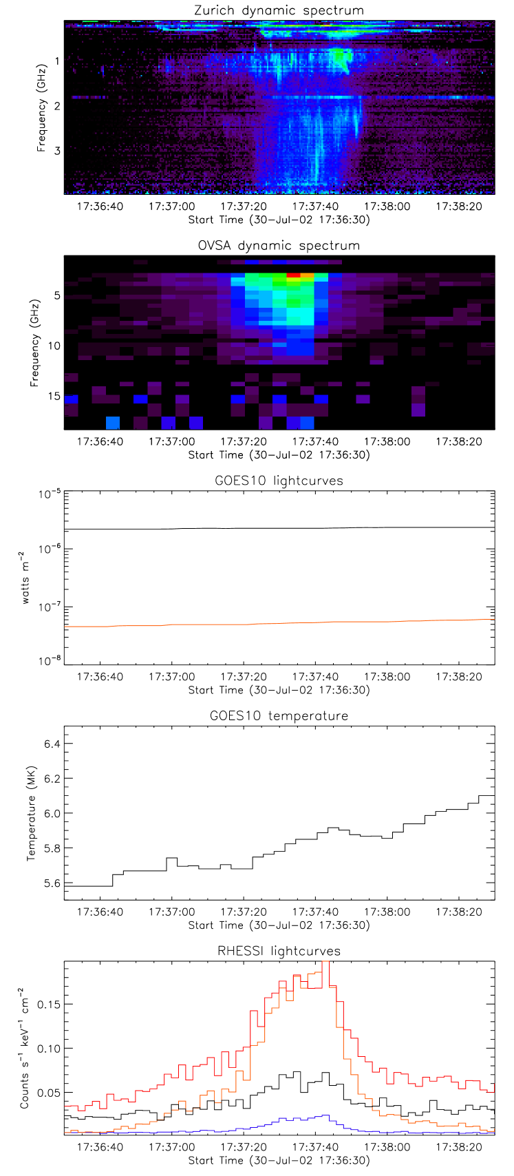
Figure 1.— Overview of July 30, 2002 flare: Phoenix-2 and OVSA dynamic spectra, top panels. GOES (3 s) lightcurves and temperature as measured by GOES-10 spacecraft assuming photospheric abundances from CHIANTI v5.2 (middle panels). RHESSI (2 second bins) lightcurves (bottom panel) in: 3-9 keV (black), 9-15 keV (red), 15-30 keV (orange), 30-100 keV (blue).

The spatially integrated RHESSI (Lin et al., 2002) X-ray spectrum (Figure  2) over the duration of the peak of the flare indicates strong non-thermal emission above $6$ keV and very weak or no thermal emission. Spectral analysis (for spectroscopy, detectors 2 and 7 were avoided) was done using OSPEX (Schwartz et al., 2002) with systematic errors set to zero (e.g. Su et al., 2009). Since the flare was close to the disk center (heliocentric angle $\sim 20^{o}$), albedo correction was applied (Kontar et al., 2006) assuming isotropic emission and hence minimum correction. The spectrum was fitted with the standard thermal plus non-thermal thick-target model (Brown, 1971) with $\chi^{2}{\sim}0.7$ (Figure  2). Bremsstrahlung cross-section following Haug (1997) has been utilized (Brown et al., 2006). However, given the clear lack of the thermal emission attributes in the event, we also used a purely non-thermal fit and found that the count spectrum can be nearly as well-fitted ($\delta_{x}{\sim}3.55$) without any thermal component, $\chi^{2}\sim 1.8$ (Figure  2).

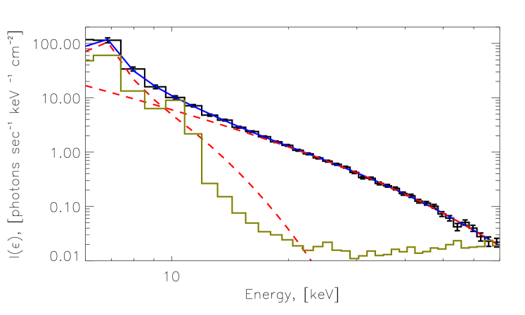
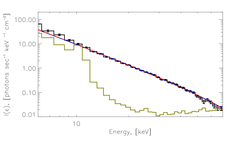
Figure 2.— RHESSI X-ray spectrum (black) above 6 keV near the peak of the event from $17:37:30-17:37:44$ UT using thermal (red-dashed) and thick-target model (red-dashed) (top panel) with best fit (blue) parameters: emission measure $EM=9.7\times 10^{45}$ cm^-3, temperature $16$ MK, $N_{e}(>6keV)=2.7\times 10^{35}$ s^-1, $\delta_{x}=3.56$. Thick-target model only (bottom panel): $N_{e}(>6keV)=2.8\times 10^{35}$ s^-1, $\delta_{x}=3.56$. The pre-flare background is shown in brown.

We have considered the variation of spectral parameters over time using the thick-target model and fitting data above 10 keV (strong background below 10 keV does not allow reliable time-dependent fit at lower energies, Figure  2). Both the number of accelerated electrons and the spectral index demonstrate typical soft-hard-soft behavior (e.g. Dennis, 1985). The hardest electron spectra $\delta_{x}{\sim}3.5$ are reached around $17:37:40$ UT. At the same time, the electron acceleration rate has its maximum $F_{e\max}(>10keV){\simeq}10^{35}$ electrons per second.

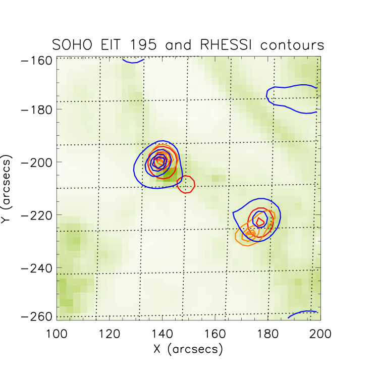
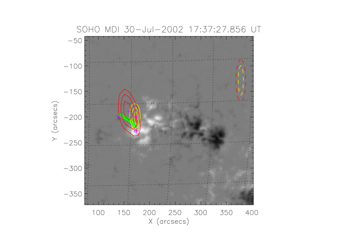
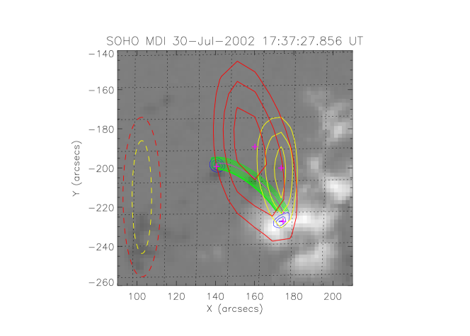
Figure 3.— Top panel: Spatial distribution of X-ray emission from July 30, 2002 flare in various energy ranges contours at 30, 50, 70, 90% levels: $9-15$ keV (red) $15-30$ keV (orange), $30-100$ keV (blue). Time accumulation interval for RHESSI images is $17:37-17:38$ UT. Background image is SoHO EIT 195 taken just before the flare at $17:36$ UT. Middle and bottom panels: the full and close-up view of the active region and a potential flux tube (green) connecting two X-ray footpoints (blue contours), $2.6-3.2$ GHz radio image (red contours) and $4.2-8.2$ GHz (yellow contours). Magenta plus signs mark the spatial peaks of the HXR and radio sources. Dashed ellipses display the sizes of the synthesized beams.

X-ray image reconstruction (Hurford et al., 2002) performed with Pixon algorithm (Pina & Puetter, 1993) shows that the flare has two well defined footpoints (Figure  3), which are well visible over the entire range of the X-ray spectrum $6-80$ keV. The imaging below $10$ keV does not demonstrate any thermal component in a separate location as is often seen at the top of a loop in flares (Kosugi et al., 1992; Aschwanden et al., 2002; Emslie et al., 2003; Kontar et al., 2008), so all the detectable X-ray emission down to the lowest energy $\sim 6$ keV comes from the footpoints. The flare occurred at the extreme eastern edge of the active region (Figure  3) with the weaker X-ray source projected onto the photosphere in a region of strong positive magnetic field, while the stronger X-ray source projects onto a small region of weaker negative magnetic field, as has commonly been observed from asymmetric flaring loops.

OVSA radio imaging for this flare is limited because only four (of six) antennas (two big and two small antennas) recorded the radio emission at the time of flare. To improve the image quality a frequency synthesis in two separate bands, $2.6-3.2$ GHz and $4.2-8.2$ GHz, with the synthesized beam sizes of $19^{\prime\prime}\times 81^{\prime\prime}$ and $10^{\prime\prime}\times 58^{\prime\prime}$, respectively, was used. This suggests that the both low- and high-frequency radio sources are unresolved. The corresponding radio images (Figure  3) are located between the X-ray footpoints although with an offset from their connecting line, which is consistent with the radio sources placement in a coronal part of a magnetic loop connecting the X-ray footpoints. The higher-frequency radio source is displaced compared with the lower-frequency one towards the stronger magnetic field (weaker X-ray) footpoint. No spatial displacement with time is detected for either of the radio sources. Based on the source separation, implied magnetic topology, and the northern HXR source size, in what follows we adopt the area of $10^{\prime\prime}$(transverse the loop)$\times 15^{\prime\prime}$(along the loop), and the depth of $10^{\prime\prime}$ for the lower-frequency radio source, which suggests the radio source volume of $V_{radio}\sim 6\times 10^{26}$ cm³, and roughly half of that for transverse sizes of the higher-frequency source.

3. Data Analysis

Generally, GS continuum radio emission can be produced by any of (i) a magnetically trapped component (trap-plus-precipitation model, Melrose & Brown, 1976), or (ii) a precipitating component, or (iii) the primary component within the acceleration region.

These three populations of fast electrons produce radio emission with distinctly different characteristics. Indeed, (i) in the case of magnetic trapping the electrons are accumulated at the looptop (Melnikov et al., 2002), and the radio light curves are delayed by roughly the trapping time $\tau_{trap}$ relative to accelerator/X-ray light curves. (ii) In the case of free electron propagation, untrapped precipitating electrons are more evenly distributed in a tenuous loop, and no delay longer than $L/v$ is expected. However, even with a roughly uniform electron distribution, most of the radio emission comes from loop regions with the strongest magnetic field. Spectral indices of the radio- and X-ray- producing fast electrons differ by 1/2 from each other, because $L/v{\propto}E^{-1/2}$. (iii) In the case of radio emission from the acceleration region, even though the residence time ($\tau_{l}$) that fast electrons spend in the acceleration region can be relatively long, the radio and X-ray light curves are proportional to each other simply because the flux of the X-ray producing electrons is equivalent to the electron loss rate from the acceleration region, $F_{e}(t)=N_{r}(t)/\tau_{l}$.

Figure 4.— RHESSI 30-100 keV (thick line) and Phoenix-2 3.2 to 3.6 GHz (thin line) lightcurves of July 30, 2002 flare with 2 s time resolution both. The  light curves are highly correlated; no significant delay is present: the lag correlation plot is given in the insert; negative delay means the radio emission comes first.

The analysis of the radio data requires, therefore, (in addition to the electron injection rate and spectrum derived from RHESSI) some information of the fast electron residence time at the radio source. To address the timing, we use Phoenix-2 (rather than the OVSA) data because of its higher time resolution. We select the frequency range of 3.2 to 3.6 GHz corresponding to the optically thin part of the radio spectrum and almost free of fine structures and interference, see Figure  1. The cross-correlation (Figure  4) displays clearly that the radio and HXR light curves are very similar to each other and there is no measurable delay in the radio component. In fact, the cross-correlation is consistent with the radio emission peaking $\sim 130$ ms earlier. The lack of noticeable delay between the radio and X-ray light curves is further confirmed by considering the OVSA light curves (4 s time resolution) at different optically thin frequencies. Therefore, the magnetically trapped electron component appears to be absent, and the radio emission is formed by either (ii) precipitating electrons or (iii) electrons in the acceleration region or both.

With the spectrum of energetic electrons from HXR data, it is easy to estimate the radio emission produced by the precipitating electron component. Taking the electron flux, the  spectral index of the radio-producing electrons $\delta_{r}{\approx}\delta_{x}+1/2$, and the electron lifetime at the loop $L/v$ (the time of flight), we can vary the magnetic field at the source in an attempt to match the spectrum shape and flux level. However, if we match the spectrum peak position, we strongly underestimate the radio flux, while if we match the flux level at the peak frequency or at an optically thin frequency, we overestimate the spectrum peak frequency; examples of such spectra are given in Figure  5 by the dotted curves. We conclude that precipitating electrons only [option (ii)] cannot make a dominant contribution to the observed radio spectrum.

Figure 5.— OVSA radio spectra obtained by two small antennas (pluses and asterisks; differences between them offer an idea about the data scatter vs frequency) and model GS emission from the acceleration region (dashed lines), precipitating electrons (dotted lines), and sum of these components (solid line). Total number and number density of the fast electrons at the radio source as derived from the OVSA radio spectrum.

To quantify the third option, we have to consider further constraints to estimate the electron residence time in the main radio source. On one hand, this residence time must be shorter than the radio light curve decay time, $\sim 10$ s; otherwise, the decay of the radio emission would be longer than observed. On the other hand, the extremely low frequency of the microwave spectrum peak implies the magnetic field is well below $100$ G at the radio source, i.e., much smaller than the footpoint magnetic field values ($\sim-130$ G and $\sim+1000$ G). This implies that the residence time in the main radio source must be noticeably larger than the time of flight, which is a fraction of second: otherwise, the fast electron density would be evenly distributed over the loop and the gyrosynchrotron (GS) microwave emission would be dominantly produced at the large field regions, resulting in a spectrum with much higher peak frequency than the observed one (as in the already considered case of the precipitating electron population). Thus, a reasonable estimate of this lifetime is somewhere between those two extremes, $\tau_{l}\sim 3$ s.

The quality of the OVSA data available for this event appears insufficient to perform a complete forward fit with all model parameters being free (Fleishman et al., 2009), which would require better calibrated imaging spectroscopy data. Instead, we have to fix as many parameters as possible (Bastian et al., 2007; Altyntsev et al., 2008) and estimate one or two remaining parameters from the fit. To do so we adopt the maximum total electron number $N_{r\max}(>6keV)=\tau_{l}F_{e\max}(>6keV)$ with a value of $F_{e\max}(>6keV)=2\times 10^{35}$ electrons/s and $\tau_{l}=3$ s, and the time evolution of $N_{r}(>6keV)$ to be proportional to an optically thin gyrosynchrotron light curve. The total lifetime of the electrons in the flaring loop is a sum of the residence time at the radio source and the time of flight between the radio source and the footpoints. As we adopted a constant, energy-independent, electron lifetime $\tau_{l}$ to be much larger than the time of flight ${\sim}L/v$ we have to accept for consistency that the spectral index of the radio emitting fast electrons is roughly the same as the spectral index of HXR emitting fast electrons determined above, $\delta_{r}=3.5$. The radio source sizes are taken as estimated in § 2. The thermal electron number density is adopted to be $n_{th}=1.5\times 10^{9}$ cm^-3 (see the next section); the GS spectra are not sensitive to this parameter until $n_{th}\lesssim 2\times 10^{9}$ cm^-3. The remaining radio source parameter, not constrained by other observations, is the magnetic field $B$, which is determined by comparing the observed (symbols) microwave and calculated (dashed curves) GS spectra (Fleishman & Kuznetsov, 2010) in Figure  5. Remarkably, that the whole time sequence of the radio spectra is reasonably fitted with a single magnetic field strength of $B\approx 60$ G; the only source parameter changing with time is the instantaneous number of the fast electrons, see Figure  5. The OVSA spectra, however, deviate from the model dashed curves by the presence of a higher-frequency bump at $f\sim 4-8$ GHz. Nevertheless, adding the contribution produced by precipitating electrons (dotted curves) at a larger magnetic field strength $B_{leg}$ peaking somewhere at the western leg (60G$<B_{leg}<$1000G) of the  loop (perhaps, around the mirror point) as follows from the OVSA imaging, Figure  3, offers a nice, consistent overall fit (solid curves) to the spectra. We conclude that the radio spectrum is dominated by the GS emission from the electron acceleration region with a distinct weaker contribution from the precipitating electrons.

4. Discussion

In order to complete a model for this cold flare event we have to estimate the flaring loop geometry. As a zero-order approximation we utilize a potential field extrapolation (Rudenko, 2001) based on the SoHO/MDI line-of-sight magnetogram. Figure  3 shows that there is a flux tube connecting the two X-ray footpoints, which confirms the existence of the required magnetic connectivity. This magnetic loop is highly asymmetric with the magnetic field reaching its minimum value (around 130 G) at the northern footpoint (stronger X-ray source). The length of the central field line is about $55^{\prime\prime}\approx 4\times 10^{9}$ cm. We know, however, that the flare phenomenon requires a non-potential magnetic loop. Furthermore, the magnetic field at the radio source (which is likely to belong to the same magnetic structure because of excellent light curve correlation) is below 100 G, which is likely to be located higher than the potential loop in Figure  3. We, therefore, propose that the true flaring loop is higher and the length of the central field line is somewhat longer; for the estimate we adopt $L\sim 100^{\prime\prime}\sim 7\times 10^{9}$ cm that yields the loop volume $V_{loop}\sim 4\times 10^{27}$ cm³ roughly 5 times larger than the radio source volume.

The next needed step is an estimate of the thermal density in the flaring loop. From the radio spectra and from the absence of any coronal X-ray source we already know that this density is low. In fact, both radio and X-ray data can be fit without any thermal plasma at all. Let us consider the 10keV electron Coulomb losses to quantify the thermal density. The collisional lifetime of the fast electrons is $t_{E}\approx 20E_{100}^{3/2}n_{10}^{-1}$ s (Bastian et al., 2007), which yields $t_{10keV}\lesssim 3$ s for the background plasma density $n_{th}\gtrsim 2\times 10^{9}$ cm^-3, which would imply the presence of a coronal 10keV X-ray component in contradiction with observations. We conclude that $2\times 10^{9}$ cm^-3 is an upper bound for the thermal electron density. To estimate the lower bound of the density, we consider the efficiency of the electron accelerator. From the X-ray fit we know that the peak acceleration efficiency is at least $F_{e\max}(>6keV)\sim 2{\times}10^{35}$ electrons per second. The duration of the flare at the half of the peak level is about $t_{1/2}\approx 25$ s, thus the total number of accelerated electrons is $N_{tot}{\sim}t_{1/2}F_{e\max}\sim\hskip 2.84544pt5\times 10^{36}$. These electrons must apparently be taken from the thermal electrons available in the flaring loop prior to the flare, thus, the ratio of $N_{tot}/V_{loop}{\sim}10^{9}$ cm^-3 represents a lower bound of the thermal electron density. These estimates justify the $n_{th}$ value adopted in the previous section.

Let us proceed now to the energy release and plasma heating efficiency. The energy release rate $dW/dt$ is estimated as the product of the minimum energy (6keV) and the acceleration rate $F_{e}(>6keV)$, which yields $\sim 2\times 10^{27}$ ergs/s at the flare peak time. Being evenly distributed over the loop volume this corresponds to the averaged density of the energy release of $\sim 0.5$ erg/cm^-3/s and, being multiplied by the effective duration $t_{1/2}$, the energy density deposition of $w\sim 12$ erg/cm^-3. Most of this energy is produced in the form of accelerated electrons around 10 keV. During the time of flight in the loop (with density $1.5\times 10^{9}$ cm^-3 and half length $\sim 3\times 10^{9}$ cm) these electrons lose about $\Delta\simeq 15\%$ of their initial energy. Thus, we can estimate the plasma heating by the accelerated electrons up to $T{\simeq}w/(k_{B}n_{th})\times\Delta\sim 7$ MK, where $k_{B}$ is the Boltzman constant. Combined with a relatively low emission measure of the tenuous loop, this heating is undetectable by GOES and RHESSI, even though the acceleration efficiency is extremely high.

Many acceleration mechanisms require the particles to be confined in the acceleration region. In particular, this is the case for acceleration in collapsing magnetic traps (e.g. Brown & Hoyng, 1975; Somov & Kosugi, 1997; Karlický & Kosugi, 2004) and for stochastic acceleration (e.g. Larosa & Moore, 1993; Miller et al., 1996; Bykov & Fleishman, 2009; Bian et al., 2010), but not for a DC field acceleration. This flare does not display any characteristics expected for the collapsing trap scenario (e.g., a spatial displacement of the source, the magnetic field growth, the radio peak frequency increase, or a time delay between radio light curves at different frequencies; Li & Fleishman, 2009), while it is consistent with the stochastic acceleration (Park & Fleishman, 2010) in a magnetic loop, when a standard, relatively narrowband, GS emission is produced at a given volume (permitted with a loop magnetic field) by the electrons accelerated there by a turbulence, whose side effect is to enhance the electron trapping and so increase, as observed, their residence time at the  acceleration region. We conclude that detection of GS radio emission from a region of stochastic acceleration of electrons is likely in the event under study. Various stochastic acceleration scenarios differ from each other in some predictions, and so in principle are distinguishable by observations. One of them is the energy dependence of the fast electron lifetime at the acceleration region. Our data are consistent with $\tau_{l}(E)=const$, which is the case, in particular, for acceleration by strong turbulence (Bykov & Fleishman, 2009). However, the precision of this constancy is insufficient in our observations to exclude competing versions of the stochastic acceleration.

What is special about this flare, which allowed detecting the radio emission from the acceleration region, compared with other flares where the radio emission is often dominated by trapped population of fast electrons? Possibly, an important aspect is the exceptional asymmetry of the flare loop; recall that the corresponding potential loop displays the minimum strength of the magnetic field absolute value at the northern photospheric footpoint (rather than coronal level), making the magnetic trapping of fast electrons totally inefficient in this case. A further important point is the somewhat low initial plasma density of the loop. This low density maintains relatively low coronal Coulomb losses of the accelerated electrons, which allows them to freely stream towards the chromosphere to produce the X-ray emission. In addition, the low density cannot supply the accelerator with seed electrons longer than half a minute or so, thus, the accelerator becomes exhausted very quickly, before the energy needed for substantial (measurable) plasma heating has been released. This explains why the main plasma remains relatively cold although the acceleration efficiency is exceptionally high (almost all available electrons are being eventually accelerated).

5. Conclusions

We have reported the observations and analysis of a cold, tenuous flare, which displays prominent and numerous non-thermal signatures, while not showing any evidence for thermal plasma heating or chromospheric evaporation. A highly asymmetric flaring loop, combined with rather low thermal electron density, made it possible to detect the GS radio emission directly from the acceleration site. We found that the electron acceleration efficiency is very high in the flare, so almost all available thermal electrons are eventually accelerated. Some sort of stochastic acceleration process is needed to account for an approximately energy-independent lifetime of about 3 s for the electrons in the acceleration region. We emphasize that the numbers derived for the quantity of accelerated electrons offer a lower bound for this measure because for our estimates we adopted a lower bound of the electron flux ($F_{e\max}(>6keV)\simeq 2\times 10^{35}$ electrons per second) and lowest electron spectral index ($\delta_{r}=3.5$) compatible with the HXR fit; taking mean values would result in even more powerful acceleration. However, given a relatively small flaring volume and rather low thermal density at the flaring loop, the total energy release turned out to be insufficient for a significant heating of the coronal plasma or for a prominent chromospheric response giving rise to chromospheric evaporation.

References

- Altyntsev et al. (2008) Altyntsev, A. T., Fleishman, G. D., Huang, G.-L., & Melnikov, V. F. 2008, ApJ, 677, 1367
- Aschwanden et al. (2002) Aschwanden, M. J., Brown, J. C., & Kontar, E. P. 2002, Sol. Phys., 210, 383
- Bastian et al. (2007) Bastian, T. S., Fleishman, G. D., & Gary, D. E. 2007, ApJ, 666, 1256
- Bian et al. (2010) Bian, N. H., Kontar, E. P., & Brown, J. C. 2010, A&A, 519, A114
- Brown (1971) Brown, J. C. 1971, Sol. Phys., 18, 489
- Brown et al. (2006) Brown, J. C., Emslie, A. G., Holman, G. D., Johns-Krull, C. M., Kontar, E. P., Lin, R. P., Massone, A. M., & Piana, M. 2006, ApJ, 643, 523
- Brown & Hoyng (1975) Brown, J. C. & Hoyng, P. 1975, ApJ, 200, 734
- Brown et al. (2007) Brown, J. C., Kontar, E. P., & Veronig, A. M. 2007, in Lecture Notes in Physics, Berlin Springer Verlag, Vol. 725, Lecture Notes in Physics, Berlin Springer Verlag, ed. K.-L. Klein & A. L. MacKinnon, 65
- Bykov & Fleishman (2009) Bykov, A. M. & Fleishman, G. D. 2009, ApJ, 692, L45
- Dennis (1985) Dennis, B. R. 1985, Sol. Phys., 100, 465
- Emslie et al. (2003) Emslie, A. G., Kontar, E. P., Krucker, S., & Lin, R. P. 2003, ApJ, 595, L107
- Fleishman & Kuznetsov (2010) Fleishman, G. D. & Kuznetsov, A. A. 2010, ApJ, 721, 1127
- Fleishman et al. (2009) Fleishman, G. D., Nita, G. M., & Gary, D. E. 2009, ApJ, 698, L183
- Haug (1997) Haug, E. 1997, A&A, 326, 417
- Hurford et al. (2002) Hurford, G. J., Schmahl, E. J., Schwartz, R. A., Conway, A. J., Aschwanden, M. J., Csillaghy, A., Dennis, B. R., Johns-Krull, C., Krucker, S., Lin, R. P., McTiernan, J., Metcalf, T. R., Sato, J., & Smith, D. M. 2002, Sol. Phys., 210, 61
- Karlický & Kosugi (2004) Karlický, M. & Kosugi, T. 2004, A&A, 419, 1159
- Kontar et al. (2008) Kontar, E. P., Hannah, I. G., & MacKinnon, A. L. 2008, A&A, 489, L57
- Kontar et al. (2006) Kontar, E. P., MacKinnon, A. L., Schwartz, R. A., & Brown, J. C. 2006, A&A, 446, 1157
- Kosugi et al. (1992) Kosugi, T., Sakao, T., Masuda, S., Makishima, K., Inda, M., Murakami, T., Ogawara, Y., Yaji, K., & Matsushita, K. 1992, PASJ, 44, L45
- Krucker et al. (2010) Krucker, S., Hudson, H. S., Glesener, L., White, S. M., Masuda, S., Wuelser, J., & Lin, R. P. 2010, ApJ, 714, 1108
- Krucker & Lin (2008) Krucker, S. & Lin, R. P. 2008, ApJ, 673, 1181
- Larosa & Moore (1993) Larosa, T. N. & Moore, R. L. 1993, ApJ, 418, 912
- Li & Fleishman (2009) Li, Y. & Fleishman, G. D. 2009, ApJ, 701, L52
- Lin et al. (2002) Lin, R. P. et al, 2002, Sol. Phys., 210, 3
- Lin et al. (2003) Lin, R. P., Krucker, S., Hurford, G. J., Smith, D. M., Hudson, H. S., Holman, G. D., Schwartz, R. A., Dennis, B. R., Share, G. H., Murphy, R. J., Emslie, A. G., Johns-Krull, C., & Vilmer, N. 2003, ApJ, 595, L69
- Melnikov et al. (2002) Melnikov, V. F., Shibasaki, K., & Reznikova, V. E. 2002, ApJ, 580, L185
- Melrose & Brown (1976) Melrose, D. B. & Brown, J. C. 1976, MNRAS, 176, 15
- Messmer et al. (1999) Messmer, P., Benz, A. O., & Monstein, C. 1999, Sol. Phys., 187, 335
- Miller et al. (1996) Miller, J. A., Larosa, T. N., & Moore, R. L. 1996, ApJ, 461, 445
- Park & Fleishman (2010) Park, S. & Fleishman, G. D. 2010, Sol. Phys., 266, 323
- Pina & Puetter (1993) Pina, R. K. & Puetter, R. C. 1993, PASP, 105, 630
- Rudenko (2001) Rudenko, G. V. 2001, Sol. Phys., 198, 5
- Schwartz et al. (2002) Schwartz, R. A., Csillaghy, A., Tolbert, A. K., Hurford, G. J., Mc Tiernan, J., & Zarro, D. 2002, Sol. Phys., 210, 165
- Somov & Kosugi (1997) Somov, B. V. & Kosugi, T. 1997, ApJ, 485, 859
- Su et al. (2009) Su, Y., Holman, G. D., Dennis, B. R., Tolbert, A. K., & Schwartz, R. A. 2009, ApJ, 705, 1584