Abstract

PPAD refers to a class of computational problems for which solutions are guaranteed to exist due to a specific combinatorial principle. The most well-known such problem is that of computing a Nash equilibrium of a game. Other examples include the search for market equilibria, and envy-free allocations in the context of cake-cutting. A problem is said to be complete for PPAD if it belongs to PPAD and can be shown to constitute one of the hardest computational challenges within that class.

In this paper, I give a relatively informal overview of the proofs used in the PPAD-completeness results. The focus is on the mixed Nash equilibria guaranteed to exist by Nash’s theorem. I also give an overview of some recent work that uses these ideas to show PSPACE-completeness for the computation of specific equilibria found by homotopy methods. I give a brief introduction to related problems of searching for market equilibria.

1 Total Search Problems

Suppose that you enter a maze without knowing anything in advance about its internal structure. Let us assume that it has only one entrance. To solve the maze, we do not ask to find some central chamber whose existence has been promised by the designer. Instead you need to find either a dead end, or else a place where the path splits, giving you a choice of which way to go; see Figure 1. Observe that this kind of solution is guaranteed to exist, and does not require any kind of promise. This is because, if there are no places where the explorer has a choice, then the interior of the maze (at least, the parts accessible from the entrance) is, topologically, a single path leading to a dead end. If you are asked to find either a dead end or a split of a path, this is informally an example of a (syntactic) total search problem — the problem description has been set up so as to guarantee that there exists a solution; the word “total” refers to the fact that every problem instance has a solution.

A maze of the sort in Figure 1 could of course be solved in linear time by checking each location. Consider now a more challenging problem defined as follows:

Definition 1.1

Circuit maze is a search problem on a $2^{n}\times 2^{n}$ grid — the maze is specified using a boolean circuit $C$ that takes as input a bit string of length $O(n)$ that represents the location (coordinates) of a possible wall or barrier between 2 adjacent grid points. $C$ has a single output bit that indicates whether in fact a barrier exists at that location.

A naive search for a grid point that corresponds to a dead end or a split of a path is no longer feasible, so the search problem becomes nontrivial. Notice that not only must some solution exist, but in addition it is easy to use $C$ to check the validity of a claimed solution.

The problem of finding, or computing, a Nash equilibrium of a game (defined in Section 3) is analogous. Nash’s theorem [53] assures us in advance that every game has a Nash equilibrium, and ultimately it works by applying a similar combinatorial principle (explained below) to the one that is being used to assure ourselves that maze problems of the sort defined above must have a solution.

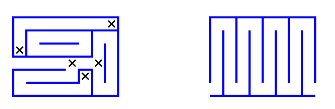
Figure 1: The left-hand maze (with a single entrance on the left) has 5 solutions marked with crosses. Note that while solutions need not be accessible starting from the entrance, at least one will be accessible. The right-hand maze illustrates how there need not be any solutions when there are 2 entrances. In general, an odd number of entrances guarantees the existence of a solution.

1.1 NP Total Search Problems

Why can we not apply a more standard notion of computational hardness, such as NP-hardness, to the problem of Nash equilibrium computation? It turns out to be due precisely to its special status as a total  search problem, as informally defined above.

Standard NP-hard problems do indeed have associated optimisation problems that are total search problems, but they are not NP total search problems. Consider for example the (NP-complete) travelling salesman problem, commonly denoted TSP. This has an associated optimisation problem, in which we seek a tour of minimal length that visits all the cities. By definition, such a minimal-length tour must exist, so this total search problem is NP-hard. But it is not, as far as we know, a member of NP — given a solution there is no obvious efficient way to check its optimality.

The complexity class PPAD (along with related classes introduced by Papadimitriou [57]) was intended to capture the computational complexity of a relatively small number of problems that seem not to have polynomial-time algorithms, but where there is a mathematical guarantee that every instance has a solution, and furthermore, given a solution, the validity of that solution may be checked in polynomial time. Each class of problems (see Section 1.3) has an associated combinatorial principle that guarantees that one has a total search problem.

A simple result due to Megiddo [51] shows that if such a problem is NP-complete, then NP would have to be equal to co-NP— it is proved as follows.

Suppose we have a reduction from any NP-hard problem (e.g. sat) to any NP total search problem (e.g. Nash). Thus, from any sat-instance (a propositional formula) we can efficiently construct a Nash-instance (a game) so that given any solution (Nash equilibrium) to that Nash-instance we can (efficiently) derive an answer to the sat-instance. That reduction could then be used to construct a nondeterministic algorithm for verifying that an unsatisfiable instance of sat indeed has no solution: Just guess a solution of the Nash-instance, and check that it indeed fails to identify a solution for the sat-instance.

The existence of such a nondeterministic algorithm for sat (one that can verify that an unsatisfiable formula is indeed unsatisfiable, hence implying that NP=co-NP) is an eventuality that is considered by complexity theorists almost as unlikely as P=NP. We conclude that Nash is very unlikely to be NP-complete.

1.2 Reducibility among total search problems

Suppose we have two total search problems $X$ and $Y$. We say that $X$ is reducible to $Y$ in polynomial time if the following holds. There should be functions $f$ and $g$ both computable in polynomial time, such that given an instance $I_{X}$ of $X$, $f(I_{X})$ is an instance of $Y$, and given any solution $S$ to $f(I_{X})$, $g(S)$ is a solution to $I_{X}$. Thus, if we had a polynomial-time algorithm that solves $Y$, the reduction would construct a polynomial-time algorithm for $X$. So, such a reduction shows that $Y$ is “at least as hard” as $X$.

While reductions in the literature are of the above form, one could use a less restrictive definition, called a Turing reduction, in which problem $X$ reduces to problem $Y$ provided that we we can write down an algorithm that solves $X$ in polynomial time, provided that it has access to an “oracle” for problem $Y$. As a consequence, if $Y$ does in fact have a polynomial-time algorithm then so does $X$. However, the reductions used in the literature to date about total search problems, are of the more restricted type.

1.3 PPAD, and some related concepts

PPAD, introduced in [57], stands for “polynomial parity argument on a directed graph”. It is defined in terms of a rather artificial-looking problem End of the line, which is the following:

Definition 1.2

An instance of End of the line consists of two boolean circuits $S$ and $P$ each of which has $n$ inputs and $n$ outputs, such that $P(0^{n})=0^{n}\not=S(0^{n})$. Find a bit vector $x$ such that $P(S(x))\not=x$ or $S(P(x))\not=x\not=0^{n}$.

$S$ and $P$ (standing for successor and predecessor) implicitly define a digraph $G$ on $2^{n}$ vertices (bit strings of length $n$) in which each vertex has indegree and outdegree at most 1. $(v,w)$ is an arc of $G$ (directed from $v$ to $w$) if and only if $S(v)=w$ and $P(w)=v$. By construction, $0^{n}$ has indegree 0, and either has outdegree 1, or $P(S(0^{n}))\not=0^{n}$ (in which case $0^{n}$ is a solution). Notice that $G$ permits efficient local exploration (the neighbours of any vertex $v$ are easy to compute from $v$) but non-local properties are opaque. We shall refer to a graph $G$ that is represented in this way as an $(S,P)$-graph.

The “parity argument on a directed graph” refers to a more general observation: define an “odd” vertex of a graph to be one where the total number of incident edges is an odd number. Then notice that the number of odd vertices must be an even number. Indeed, this observation applies generally to undirected graphs, but we apply it here to $(S,P)$-graphs, in particular those $(S,P)$-graphs where vertex $0^{n}$ actually has an outgoing arc (so has odd degree). These $(S,P)$-graphs have an associated total search problem, of finding an alternative odd-degree vertex. One could search for such a vertex by, for example

• checking each bit string in order, looking up its neighbours to see if it’s an odd vertex, or

• following a directed path starting at some vertex; an endpoint other than $0^{n}$ must be reached,

but since $G$ is exponentially large, these naive approaches will take exponential time in the worst case.

Definition 1.3

A computational problem $X$ belong to the complexity class PPAD provided that $X$ reduces to End of the line in polynomial time. Problem $X$ is PPAD-complete provided that $X$ is in PPAD, and in addition End of the line reduces to $X$ in polynomial time.

Thus End of the line stands in the same relationship to PPAD, that Circuit sat does to NP (although NP is not actually defined in terms of Circuit sat, an equivalent definition would say that NP-complete problems are those that are polynomial-time equivalent to Circuit sat, and a member of NP is a problem that can be reduced to Circuit sat).

The above definition of PPAD is the one used in [22]; it is noted there that there are many alternative equivalent definitions. Since End of the line is by construction a total search problem, it follows that members of PPAD are necessarily also total search problems.

How hard is “PPAD-complete”?

PPAD lies “between P and NP” in the sense that if P were equal to NP, then all PPAD problems would be polynomial-time solvable, while the assumption that “PPAD-complete problems are hard” implies P not equal to NP. It is a fair criticism of these results that they do not carry as much weight as do NP-hardness results, partly for this reason, and partly because there are only a handful of PPAD-complete problems, while thousands of problems have been shown to be NP-complete.

Why, then, do we take PPAD-completeness as evidence that a problem cannot be solved in polynomial time? One argument is that End of the line is defined in terms of unrestricted circuits, and general boolean circuits seem to be hard to analyse via polynomial-time algorithms. We should also note the oracle separation results of [4] in this context.

Related complexity classes

Other combinatorial principles are considered in [57], that guarantee totality of corresponding search problems. For example, consider the pigeonhole principle, that given a function $f:X\longrightarrow Y$, if $X$ and $Y$ are finite and $|X|>|Y|$, there must exist $x,x^{\prime}\in X$ such that $f(x)=f(x^{\prime})$. Now define an associated computational problem:

Definition 1.4

The problem Pigeonhole circuit has as instances, directed boolean circuits having the same number of inputs and outputs. Let $f$ be the function computed by the circuit. The problem is to identify either two distinct bit strings $x$, $x^{\prime}$ with $f(x)=f(x^{\prime})$, or a bit string $x$ with $f(x)=0$ (where $0$ is the all-zeroes bit string).

Note that by construction, this a total search problem, and it is an NP total search problem since it is computationally easy to check that a given solution is valid. At the same time, it seems to be hard to find a solution, although it is unlikely to be NP-hard, due to Megiddo’s result. The complexity class PPP [57] (for “polynomial pigeonhole principle”) is defined as the set of all total search problems that are reducible to Pigeonhole circuit.

The pigeonhole principle is a generalisation of the parity argument on a directed graph. To see this, notice that the function $f:X\longrightarrow Y$ can map a vertex $v$ of an End of the line graph to the adjacent vertex connected by an arc from $v$, or to itself if $v$ has outdegree 0. PPAD is a subclass of PPP— End of the line reduces to Pigeonhole circuit; it would be nice to obtain a reduction the other way and show equivalence, but that has not been achieved.

If we have an undirected graph of degree at most 2 with a known endpoint, then the search for another endpoint is also a total search problem. The corresponding complexity class defined in [57] is PPA. The Circuit maze problem that we considered informally at the start, belongs to PPA. As it happens, the problem is likely to be complete for PPA.

2 Sperner’s lemma, and an associated computational problem

Sperner’s lemma is the following combinatorial result, that can be used to prove Brouwer’s fixed point theorem.

Theorem 2.1

[64] Let $\{v_{0},v_{1},\ldots,v_{d}\}$ be the vertices of a $d$-simplex $S$, and suppose that the interior of $S$ is decomposed into smaller simplices using additional vertices. Assign each vertex a colour from $\{0,1,\ldots d\}$ such that $v_{i}$ gets colour $i$, and a vertex on any face of $S$ must get one of the colours of the vertices of that face. Interior vertices may be coloured arbitrarily. Then, this simplicial decomposition must include a panchromatic simplex, i.e. one whose vertices has all distinct colours.

• The proof can be found in many places, so here we just give a sketch for the 2-dimensional case. Let us define the computational problem Sperner (discussed in more detail below) to be the problem of exhibiting a trichromatic triangle. Essentially, the proof consists of a reduction from Sperner to End of the line!

  Choose any two of the colours, say 0 and 1. We begin by adding some further triangles to the triangulation as shown in Figure 2 by the dotted lines: by adding a sequence of triangles that have the original extremal vertex coloured 1, together with two consecutive vertices on the 1-0 edge, we end up with a triangulation that has only one 0/1-coloured edge on the exterior.

  Construct a directed graph $G$ whose vertices are triangles of this extended triangulation. Add a directed edge of $G$ between any two triangles that are adjacent and separated by a 0/1-edge; the direction of the edge is so as to cross with 0 on its left and 1 on its right. Consequently, there is a single edge coming into the triangulation from the outside. It is simple to check that in $G$, trichromatic triangles correspond exactly with degree-1 vertices, solutions to End of the line. This completes the reduction.       $\square$

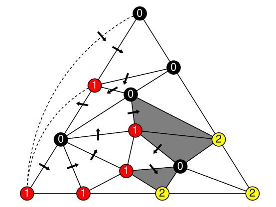
Figure 2: An example to illustrate Sperner’s lemma.
The solid lines show the triangle and the simplicisation (triangulation, since we are in 2 dimensions.) The dashed lines add an additional sequence of topological triangles along one side of the triangulation; as a result of those lines, there is only one edge coloured 0-1 when viewed from the exterior.
The arrows are the directed edges of the corresponding graph.
The shaded triangles are trichromatic (End-of-line solutions in the corresponding graph).

To define a challenging computational problem involved with searching for a panchromatic Sperner simplex, we need to work with Sperner triangulations that are represented so compactly that it becomes infeasible to just check every simplex. Hence, we consider exponentially-large simplicial decompositions that satisfy the boundary conditions required for Sperner’s lemma.

Informally, the computational problem Sperner [57] (with parameter $n$) takes as input a Sperner triangulation that contains an number of vertices that is exponential in $n$. The vertices —and their colours— cannot be explicitly listed, since problem instances are supposed to be written down with a syntactic description length that is polynomial in $n$. Instead, an instance is specified by a circuit $C$ that takes as input the coordinates of a vertex and outputs its colour. This means that the vertices should lie on a regular grid, and $C$ takes as input a bit string that represents the coordinates of a vertex.

Figure 3 shows one way to do this in 2 dimensions (assume that the central grid has exponentially-many points). There is no restriction on how $C$ may colour the vertices labelled $*$; the other labels are fixed boundary conditions to ensure that any trichromatic triangle lies within the grid. A 3-dimensional version would just require some choice of simplicial decomposition of a cube, which would then be applied to each small cube in the corresponding 3-d grid.

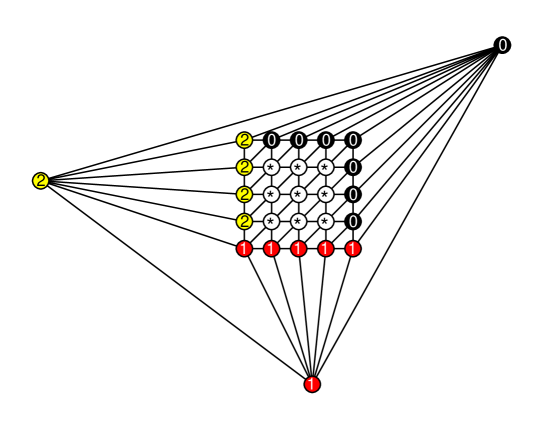
Figure 3: Embedding a triangulated grid inside an instance of Sperner’s lemma

2-dimensional Sperner is known to be PPAD-complete [10]; previously it was known from [57] that 3-dimensional Sperner is PPAD-complete. One interesting feature of the PPAD-completeness results for Nash equilibrium computation, is that normal-form games do not incorporate generic boolean circuits in an obvious way. Contrast that with Sperner as defined above, where a problem instance incorporates a generic boolean circuit to determine the colour of a vertex. We continue by explaining Nash equilibrium computation in more detail, and how it is polynomial-time equivalent to Sperner.

3 Games and Nash Equilibria

A game ${\mathcal{G}}$ specifies a finite set of $k\geq 2$ players, where each player $i$ has a finite set $S_{i}$ of (at least two) actions or pure strategies. Let $S=S_{1}\times\ldots\times S_{k}$ be the set of pure strategy profiles, thus an element of $S$ represents a choice made by each player $i$ of a single pure strategy from his set $S_{i}$. Finally, given any member of $S$, ${\mathcal{G}}$ needs to specify real-valued utilities or payoffs to each player that result from that pure strategy profile. Let $u^{i}_{s}$ denote the payoff to player $i$ that results from $s\in S$.

Informally, a Nash equilibrium is a set of strategies —one for each player— where no player has an “incentive to deviate” i.e. play some alternative strategy. After giving some examples, we provide a precise definition, along with some notation. In general, Nash equilibria do not exist for pure strategies; it is usually necessary to allow the players to randomise over them, as shown in the following examples.

Rock-paper-scissors: $$\begin{array}[]{rcccc}&\vline&rock&paper&scissors\\ \hline\cr rock&\vline&(0,0)&(-1,1)&(1,-1)\\ paper&\vline&(1,-1)&(0,0)&(-1,1)\\ scissors&\vline&(-1,1)&(1,-1)&(0,0)\\ \end{array}$$ A typical payoff matrix for Stag hunt: $$\begin{array}[]{rccc}&\vline&hunt~{}stag&hunt~{}hare\\ \hline\cr hunt~{}stag&\vline&(8,8)&(0,1)\\ hunt~{}hare&\vline&(1,0)&(1,1)\\ \end{array}$$ Generalised matching pennies: the row player “wins” (and collects a payment from the column player) whenever both players play the same strategy. $$\begin{array}[]{rccccc}&\vline&1&2&\cdots&n\\ \hline\cr 1&\vline&(1,-1)&(0,0)&\cdots&(0,0)\\ 2&\vline&(0,0)&(1,-1)&&(0,0)\\ \vdots&\vline&\vdots&&\ddots&(0,0)\\ n&\vline&(0,0)&\cdots&(0,0)&(1,-1)\\ \end{array}$$

Figure 4: Payoff matrices for example games. Each entry of a matrix contains two numbers: the row player’s payoff and the column player’s payoff.

Example 3.1

The traditional game of rock-paper-scissors fits in to the basic paradigm considered here. The standard payoff matrix shown in Figure 4 awards one point for winning and a penalty of one point for losing. The unique Nash equilibrium has both players randomising uniformly over their strategies, for an expected payoff of zero.

Example 3.2

The stag hunt game [60] has two players, each of whom has two actions, corresponding to hunting either a stag, or a hare. In order to catch a stag, both player must cooperate (choose to hunt a stag), but either player can catch a hare on his own. The benefit of hunting a stag is that the payoff (half share of a stag) is presumed to be substantially larger than an entire hare.

A typical choice of payoffs (Figure 4) to reflect this dilemma could award 8 to both players when they both hunt a stag, 0 to a player who hunts a stag while the other player hunts a hare, and 1 to a player who hunts a hare. Using these payoffs, there are 3 Nash equilibria: one where both players hunt a stag, one where both players hunt a hare, and one where each player hunts a stag with probability $\frac{1}{8}$ and a hare with probability $\frac{7}{8}$.

Example 3.3

Generalised matching pennies (Figure 4) is a useful example to present here, since it is used as an ingredient of the PPAD-completeness proof for Nash.

The game of matching pennies is a 2-player game, whose basic version has each player having just two strategies, “heads” and “tails”. The row player wins whenever both players make the same choice, otherwise the column player wins. In the original version, a win effectively means that the losing player pays one unit to the winning player; here we modify payoffs so that a win for the column player just results in zero payoffs (he avoids paying the row player). With that modification, generalised matching pennies is the extension to $n$ actions rather than just 2.

There is a unique Nash equilibrium in which both players use the uniform distribution over their pure strategies, and it is easy to see that no other solution is possible.

Comments.

The Stag Hunt example shows that there may be multiple equilibria, that some equilibria have more social welfare than others, and that some are more “plausible” that others (thus, it seems reasonable to expect one of the two pure-strategy equilibria to be played, rather than the randomised one). The topic of equilibrium selection considers formalisations of the notion of plausibility, and the problem of computing the relevant equilibria. Of course, it is at least as hard to compute one of a subset of equilibria as it is to compute an unrestricted one. For example, it is NP-complete to compute equilibria that guarantee one or both players a certain level of payoff, or that satisfy various other properties that are efficiently checkable [18, 35].

If we know the supports of a Nash equilibrium (the strategies played with non-zero probability) then it would be straightforward to compute a Nash equilibrium, since it then reduces to a linear programming problem. Thus (as noted by Papadimitriou in [55]) the search for a Nash equilibrium is —in the 2-player case— essentially a combinatorial problem.

Nash equilibrium and $\epsilon$-Nash equilibrium; definition and notation.

A mixed strategy for player $i$ is a distribution on $S_{i}$, that is, $|S_{i}|$ nonnegative real numbers summing to 1. We will use $x^{i}_{j}$ to denote the probability that player $i$ allocates to strategy $j\in S_{i}$. If some or all players use mixed strategies, this results in expected payoffs for the players. A best response by a player is a strategy (possibly mixed) that maximises that player’s expected payoff; the assumption is that players do indeed play to maximise expected payoffs.

Call a set of $k$ mixed strategies $x^{i}_{j}$ a Nash equilibrium if, for each player $i$, $i$’s expected payoff $\sum_{s\in S}u^{i}_{s}\prod_{r=1}^{k}x^{r}_{s_{r}}$ is maximized over all mixed strategies of $i$. That is, a Nash equilibrium is a set of mixed strategies from which no player has an incentive to deviate. Let $S_{-i}=S_{1}\times\ldots\times S_{i-1}\times S_{i+1}\times\ldots\times S_{k}$, the set of pure strategy profiles of players other than $i$. For $s\in S_{-i}$, let $x_{s}=\prod_{r\not=i;r\in[k]}x^{r}_{s_{r}}$ and $u^{i}_{js}$ be the payoff to $i$ when $i$ plays $j$ and the other players play $s$. It is well-known (see, e.g., [56]) that the following is an equivalent condition for a set of mixed strategies to be a Nash equilibrium:

$$\forall i,j,j^{\prime}\sum_{s\in S_{-i}}u^{i}_{js}x_{s}>\sum_{s\in S_{-i}}u^{i}_{j^{\prime}s}x_{s}\Longrightarrow x^{i}_{j^{\prime}}=0.$$ (3.1)

Also, a set of mixed strategies is an $\epsilon$-Nash equilibrium for some $\epsilon>0$ if the following holds:

$$\forall i,j,j^{\prime}\sum_{s\in S_{-i}}u^{i}_{js}x_{s}>\sum_{s\in S_{-i}}u^{i}_{j^{\prime}s}x_{s}+\epsilon\Longrightarrow x^{i}_{j^{\prime}}=0.$$ (3.2)

The celebrated theorem of Nash [53] states that every game has a Nash equilibrium.

Comments.

An $\epsilon$-Nash equilibrium is a weaker notion than a Nash equilibrium; a Nash equilibrium is an $\epsilon$-Nash equilibrium for $\epsilon=0$, and generally an $\epsilon$-Nash equilibrium is an $\epsilon^{\prime}$-Nash equilibrium for any $\epsilon^{\prime}>\epsilon$.

Why focus on approximate equilibria?

Approximate equilibria matter from the computational perspective, because for games of more than 2 players, a solution (Nash equilibrium) may be in irrational numbers, even when the utilities $u^{i}_{s}$ that specify a game, are themselves rational numbers [53]. The problem of computing a Nash equilibrium —as opposed to just knowing that one exists— requires us to specify a format or syntax in which to output the quantities that make up a solution (i.e. the probabilities $x^{i}_{s}$).

In [23] (an expository paper on the results of [22]) we noted an analogy between equilibrium computation and the computation of a root of an odd-degree polynomial $f$ in a single variable. For both problems, there is a guarantee that a solution really exists, and the guarantee is based on the nature of the problem rather than a promise that the given instance has a solution. Furthermore, in each problem we have to deal with the issue of how to represent a solution, since a solution need not necessarily be a rational number. And, in both cases a natural approach is to switch to some notion of approximate solution: instead of searching for $x$ with $f(x)=0$, search for $x$ with $|f(x)|<\epsilon$, which ensures that $x$ can be written down in a standard syntax.

3.1 Some reductions among equilibrium problems

By way of example, consider the well-known result (that predates the PPAD-hardness of Nash; see [55] Chapter 2 for further background) that symmetric 2-player games are as hard to solve as general ones.

Given a $n\times n$ game ${\mathcal{G}}$, construct a symmetric $2n\times 2n$ game ${\mathcal{G}}^{\prime}=f({\mathcal{G}})$, such that given any Nash equilibrium of ${\mathcal{G}}^{\prime}$ we can efficiently reconstruct a Nash equilibrium of ${\mathcal{G}}$. To begin, let us assume that all payoffs in ${\mathcal{G}}$ are positive — the reason why this assumption is fine, is that if there are any negative payoffs, then we can add a sufficiently large constant to all payoffs and obtain a strategically equivalent version (i.e. one that has the same Nash equilibria).

Now suppose we solve the $2n\times 2n$ game ${\mathcal{G}}^{\prime}=\left(\begin{array}[]{cc}0&{\mathcal{G}}\\ {\mathcal{G}}^{T}&0\end{array}\right)$, where we assume that entries contain payoffs to both players, and the zeroes represent $n\times n$ matrices of payoffs of zero to both players.

Let $p$ and $q$ denote the probabilities that players 1 and 2 use their first $n$ actions, in some given solution. If we label the rows and columns of the payoff matrix with the probabilities assigned to them by the players, we have

$$\begin{array}[]{cc}&{~{}~{}q~{}~{}~{}1-q}\\ \begin{array}[]{r}{p}\\ {1-p}\end{array}&\left(\begin{array}[]{cc}0&{\mathcal{G}}\\ {\mathcal{G}}^{T}&0\end{array}\right)\end{array}$$

If $p=q=1$, both players receive payoff 0, and both have an incentive to change their behaviour, by the assumption that ${\mathcal{G}}$’s payoffs are all positive (and similarly if $p=q=0$). So we have $p>0$ and $1-q>0$, or alternatively, $1-p>0$ and $q>0$.

Assume $p>0$ and $1-q>0$ (the analysis for the other case is similar). Let $\{{p_{1},...,p_{n}}\}$ be the probabilities used by player 1 for his first $n$ actions, $\{{q_{1},\ldots q_{n}}\}$ the probabilities for player 2’s second $n$ actions.

$$\begin{array}[]{cc}&{~{}~{}~{}q~{}~{}~{}~{}(q_{1}...q_{n})}\\ \begin{array}[]{r}{(p_{1},...p_{n})}\\ {1-p}\end{array}&\left(\begin{array}[]{cc}0&{\mathcal{G}}\\ {\mathcal{G}}^{T}&0\end{array}\right)\end{array}$$

Note that ${p_{1}+\ldots+p_{n}=p}$ and ${q_{1}+\ldots+q_{n}=1-q}$. Then ${(p_{1}/p,\ldots,p_{n}/p)}$ and ${(q_{1}/(1-q),\ldots,q_{n}/(1-q))}$ are a Nash equilibrium of ${\mathcal{G}}$. To see this, consider the diagram; they should form a best response to each other for the top-right part.

This is an example of the kind of reduction defined in Section 1.2. In the context of games, this kind of reduction is called in [1] a Nash homomorphism. Abbott et al. [1] reduce general 2-player games to win-lose 2-player games (where payoffs are 0 or 1). Various other Nash homomorphisms have been derived independently of the work relating Nash to PPAD. An important one is Bubelis [8] that reduces (in a more algebraic style) $k$-player games to 3-player games. The result also highlights a key distinction between $k$-player games (for $k\geq 3$) and 2-player games; in 2-player games the solutions are rational numbers (provided that the payoff in the games are rational) while for 3 or more players, the solutions may be irrational. The reduction of [8] preserves key algebraic properties of the quantities $x^{i}_{j}$ in a solution, such as their degree (i.e the degree of the lowest-degree polynomial with integer coefficients satisfied by $x^{i}_{j}$). Since we have noted that 2-player games have solutions in rational numbers, this kind of reduction could not apply to 2-player games.

3.2 The “in PPAD” result

A proof that Nash equilibrium computation belongs to PPAD necessarily incorporates a proof of Nash’s theorem itself (for approximate equilibrium), in that a reduction from $\epsilon$-Nash to End of the line assures us that $\epsilon$-Nash is a total search problem, since it is clear that End of the line is. To derive Nash’s theorem itself, that an exact equilibrium exists, the summary as in [57] is as follows: Consider an infinite sequence of solutions to $\epsilon$-Nash for smaller and smaller $\epsilon$. Since the space of mixed-strategy profiles is compact, these solutions have a limit point, which must be an exact solution.

3.3 The Algebraic Properties of Nash Equilibria

A reader who is interested on the combinatorial aspects of the topic can skip most of this subsection; the main point to note is that since a Nash equilibrium is not necessarily in rational numbers, this motivates the focus on approximate equilibria (i.e. $\epsilon$-Nash equilibria), to ensure that there is a natural syntax in which to output a computed solution to a game. Since any exact equilibrium is an approximate one, any hardness result for approximate equilibria applies automatically to exact ones. The question of polynomial-time computation of approximate equilibria was introduced in [37] in order to finesse the irrationality of exact solutions. However, algorithms for approximate equilibria go back earlier, notably Scarf’s algorithm [62].

For positive $\epsilon$, an $\epsilon$-Nash equilibrium need not be at all close to a true Nash equilibrium. Etessami and Yannakakis [31] show that even for exponentially small $\epsilon$, an $\epsilon$-Nash equilibrium may be at variation distance 1 from any true Nash equilibrium, for a 3-player game. Furthermore, they also show that computing an approximate equilibrium that is within variation distance $\epsilon$ from a true one (an $\epsilon$-near equilibrium) is square-root-sum hard. This refers to the following well-known computational problem:

Definition 3.4

The square root sum problem takes as input two sets of positive integers, say $\{x_{1},\ldots,x_{n}\}$ and $\{y_{1},\ldots,y_{n}\}$. The question is: is the sum of the square roots of the first set, greater than the sum of square roots of the second?

The problem is not known to belong to NP, although neither is it known to be hard for any well-known complexity class. In terms of upper-bounding the complexity of this problem, and also for that matter, computing an $\epsilon$-near equilibrium, we may note that the criteria for a set of numbers $x^{i}_{j}$ to be an $\epsilon$-near equilibrium can be expressed in the existential theory of real arithmetic, which places the problem in PSPACE [58].

The fact that Nash equilibrium probabilities can be irrational numbers (while payoffs are rational numbers) appears in an example in Nash’s paper [53]. He describes a simple poker-style game with 3 players and a unique (irrational) Nash equilibrium. We noted earlier that any game with rational payoffs has Nash equilibria probabilities that are algebraic numbers. But even for a 3-player game, if $n$ is the number of actions, the solution may require algebraic numbers of degree exponentially large in $n$; as noted in [37], the constructions introduced there give us a flexible way to construct, from a given polynomial $p$, an arithmetic circuit whose fixpoints are the roots of $p$, and [37] shows how to construct a 4-player game whose equilibria encode those fixpoints. The paper of Bubelis [8] gave an “algebraic” reduction from any $k$-player game (for $k>3$) to a corresponding 3-player game, in a way that preserves the algebraic properties of the solutions. Consequently 3-player games have the same feature of 4-player games identified in [37]. The reduction of [8] can in addition be used to show that 3-player games are as computationally hard to solve as $k$-players, but it does not highlight the expressive power of games as arithmetic circuits. Recently, Feige and Talgam-Cohen [32] give a reduction from (approximate) $k$-player Nash to 2-player Nash, that does not explicitly proceed via End of the line.

Is Nash equilibrium computation ever harder than PPAD?

Daskalakis et al. [20] show that most standard classes of concisely-represented games (such as graphical games and polymatrix games) have equilibrium computation problems that reduce to 2-Nash and so belong to PPAD. Schoenebeck and Vadhan [63] study the question for “circuit games”, a very general concise representation of games where payoffs are given by a boolean circuit. In this context they obtain hardness results, but this is not an NP total search problem. The zero-sum version [33] is also hard.

4 Brouwer functions, and discrete Brouwer functions

Brouwer’s fixpoint theorem states that every continuous function from a convex compact domain to itself, must have a fixpoint, a point $x$ for which $f(x)=x$.

Proving Brouwer’s fixpoint theorem using Sperner’s lemma

Suppose to begin with that the domain in question is the $d$-simplex $\Delta^{d}$. We have continuous $f:\Delta^{d}\longrightarrow\Delta^{d}$ and we seek a point $x\in\Delta^{d}$ with $f(x)=x$. Suppose $f$ is evaluated on a set $S$ of “sample points” in $\Delta^{d}$, and at each point $x\in S$, consider the value of $f(x)-x$. If the $d+1$ vertices of $\Delta^{d}$ are given distinct colours $\{0,1,\ldots,d\}$, we colour-code any $x\in S$ according to the direction of $f(x)-x$: we give it the colour of a vertex which is at least as distant from $f(x)$ as from $x$. Such a colouring respects the constraints of Sperner’s lemma. If $S$ is used as the vertices of a simplicial decomposition, a panchromatic simplex becomes a plausible location for a fixpoint ($f$ is displacing co-located vertices in all different directions). One obtains a fixpoint from the limit of increasingly fine simplicial decompositions.

The result can then be extended to other domains that are topologically equivalent to simplices, such as cubes/cuboids, as used in the constructions we describe here.

In defining an associated computational total search problem “find the point $x$”, we need to identify a syntax or format in which to represent a class of continuous functions. The format should ensure that $f$ can be computed in time polynomial in $f$’s description length (so that solutions $x$ are easily checkable, and the search problem is in NP). The class of functions that we define are based on discrete Brouwer functions, defined in detail below in Section 4.1.

Discrete Brouwer functions form the bridge between the discrete circuit problem End of the line and the continuous, numerical problem of computing a Nash equilibrium.

Consider the following obvious fact that if we colour the integers $\{0,\ldots,n\}$ such that

• each integer is coloured either red or black, and

• 0 is coloured red, and $n$ is coloured black

then there must be two consecutive numbers that have different colours.

Now suppose that $n$ is exponentially large, but for any number $x$ in the range $\{0,\ldots,n\}$ we have an efficient test to identify the colour of $x$. In that case, we still have an efficient search for consecutive numbers that have opposite colours, namely we can use binary search. If $\lfloor n/2\rfloor$ is coloured black, we would search for the pair of numbers in the range $\{0,\ldots,\lfloor n/2\rfloor\}$, otherwise we would search in the range $\{\lfloor n/2\rfloor,\ldots,n\}$, and so on.

Now consider a 2-dimensional version with pairs of numbers $(x,y)$, $x,y\in\{0,\ldots,n\}$, where pairs of numbers are coloured as follows.

• if $x=0$, $(x,y)$ is coloured red,

• if $y=0$ and $x>0$ then $(x,y)$ is coloured yellow,

• if $x,y>0$ and either $x=n$ or $y=n$ (or both), then $(x,y)$ is coloured black.

Thus, we have fixed the colouring of the perimeter of the grid of points, but we impose no constraints on how the interior should be coloured. We claim that there exists a square of size 1 that has all 3 colours, but notice that binary search no longer finds such a square efficiently. The fact that such a square exists is due to Sperner’s lemma, whose proof envisages following a path that enters the $n\times n$ grid, ending up at a trichromatic square; intuitively, this can be achieved by entering at the point on the perimeter where red and yellow are adjacent, and walking around the outside of the red region. Since there is only one exterior red/yellow interval, we are guaranteed to reach a stage where the red region is no longer bounded by yellow points, but by black points.

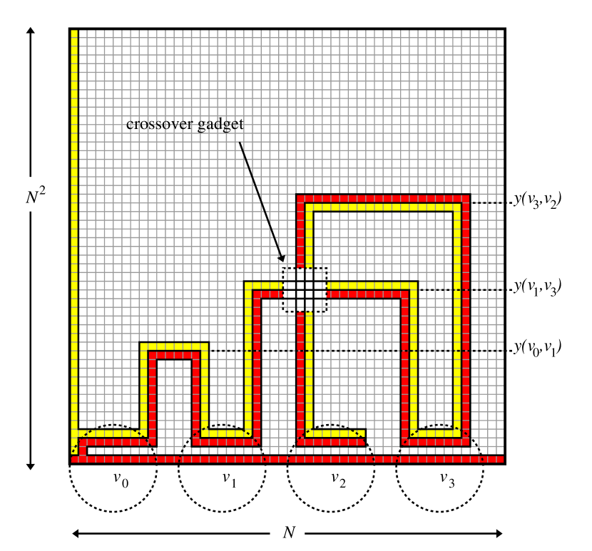
Figure 5: The figure shows how the line graph $(v_{0},v_{1}),(v_{1},v_{3}),(v_{3},v_{2})$ is encoded as a discrete Brouwer function in two dimensions.
The function colours the grid as a long thin red/yellow strip on a black background. Each vertex $v_{i}$ is associated with a horizontal line segment close to the $x$-axis (circled in the diagram). Each edge $(v_{i},v_{j})$ is associated with a “bridge” from the right-hand side of $v_{i}$’s line segment to the left-hand side of $v_{j}$’s.
Each bridge consists of three red/yellow line segments, going up, across and down. The $y$-coordinate of the horizontal segment $y(i,j)$ should efficiently encode the values $i$ and $j$ (for example, $y(i,j)=i+N.j$ where $N$ is the number of $x$-values possible).
Hence no two bridges can have overlapping horizontal sections. Unfortunately, a horizontal section may need to cross a vertical section of a different bridge, as shown in the diagram. Here a crossover gadget of [10] (Figure 6) may be used.

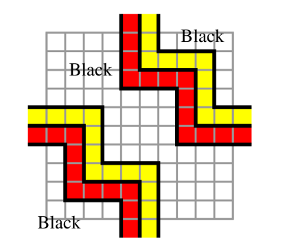
Figure 6: The crossover gadget referred to in Figure 5.
To avoid all three colours meeting in the vicinity of the crossing of two red/yellow path segments: the simple solution is to re-connect the paths in a way that the topological structure of the red-yellow line no longer mimics the structure of the End of the line graph from which it was derived. The 3-dimensional version, invented in [57] and refined in [22] does not require crossover gadgets.

4.1 Discrete Brouwer functions

We next give a detailed definition of discrete Brouwer functions (DBFs), together with an associated total search problem (on an exponential-sized domain), that is used in the reductions from End of the line to the search for a Nash equilibrium of a game. Figure 5 shows how an End of the line graph is encoded by a DBF.

Definition 4.1

Partition the unit $d$-dimensional cube $K$ into “cubelets”— $2^{dn}$ axis aligned cubes of edge length $2^{-n}$. A Brouwer-mapping circuit (in $d$ dimensions) takes as input a bit string of length $dn$ that represents the coordinates of a cubelet, and outputs its colour, subject to boundary constraints that generalise the 2-D case discussed above. A Discrete Brouwer function (DBF) is the function computed by such a circuit, and its syntactic complexity is the size of the circuit that represents it, which we restrict to be polynomial in $n$.

This gives rise to the total search problem of finding a vertex that belongs to cubelets of all the different colours (a “panchromatic cubelet”). A superficial difference between the presentation of this concept in [22] compared with [13] is that [22] associates each cubelet with a colour while [13] associated each vertex with a colour, and the search is for a cubelet that has vertices of all colours.

5 From Discrete Brouwer functions to Games

The reduction is broken down into two stages: first we take a circuit $C$ representing a DBF and encode it as an arithmetic circuit $C^{\prime}$ that computes a continuous function from $K^{d}$ to $K^{d}$, where $K^{d}$ is the $d$-dimensional unit cube. Then we express $C^{\prime}$ as a game ${\mathcal{G}}$ in such a way that given any Nash equilibrium of ${\mathcal{G}}$, we can efficiently extract the coordinates of a fixpoint of $C^{\prime}$.

Figure 7 gives the general idea of how to construct a continuous function $f$ from a DBF, in such a way that fixpoints of the continuous function correspond to solutions of the DBF. The idea is that each colour in the range of the DBF corresponds to a direction of $f(x)-x$. For a colour that lies on the boundary of the discretised cube, we choose a direction away from that boundary, so that $f$ avoids displacing points outside the cube. Indeed, this is where we require the boundary constraints on the colouring of DBFs. Points at the centres of the cubelets of the DBF will be displaced in the direction of that cubelet’s colour, while points on or near the boundary of two or more cubelets should get directions that interpolate the individual colour-directions (which is necessary for continuity). A natural choice for these colour-directions results in the following property: For a proper subset of these directions, their average cannot be zero. On the other hand, a weighted average of all the directions can indeed be zero.

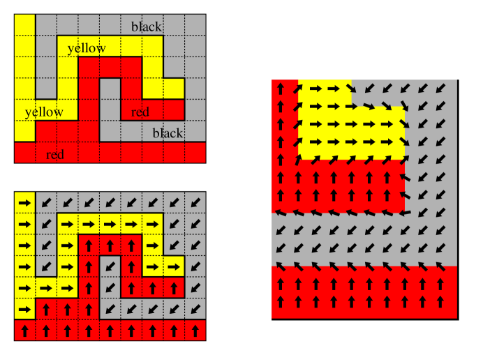
Figure 7: The top left-hand diagram shows a simple discrete Brouwer function in 2 dimensions, and the arrows in the bottom left-hand diagram show the direction of the corresponding continuous Brouwer function $f$ within each small square.
The right-hand diagram is a magnified view of the bottom right-hand section of the continuous Brouwer function, showing how the direction of the function (i.e the direction of $f(x)-x$) can be interpolated on the boundaries of the small squares.
It is always possible to smoothly interpolate between 2 different directions without introducing fixed points of $f$. But, in the vicinity of the point where all 3 colours meet, there will necessarily be a point $x$ where $f(x)=x$.

Arithmetic circuits

The papers [13, 22] show how to construct arithmetic circuits that compute these kinds of continuous functions. An arithmetic circuit consists of a directed graph each of whose nodes belongs to one of a number of distinct types, such as addition and multiplication. Each node will compute a real number, and the type of a node dictates how that number is obtained. For example, an addition node should have 2 incoming arcs, and it will compute the sum of the values located at the adjacent nodes for those two arcs; it may also have a number of outgoing arcs that allow its value to feed in to other nodes.

A significant difference between the circuits of [22] and those of [13] is that the latter do not allow nodes that compute the product of two computed quantities (located at other nodes with incoming edges). They do allow the multiplication of a computed quantity by a constant. The result of this is

• The functions that can be computed are more constrained; however they are still expressive enough to simulate the behaviour of DBF circuits,

• two-player normal-form games can simulate the circuits of [13], while three-player games are required to simulate circuits that can multiply a pair of computed quantities.

The more general circuits introduced in [22] correspond to the algebraic complexity class FIXP of Etessami and Yannakakis [31]; the ones without these product nodes correspond to PPAD, the linear version of FIXP, called LINEAR-FIXP in [31].

Interpolating the directions

For a point $x$ that is not on a cubelet boundary, one can design a polynomial-sized arithmetic circuit that compares the values of its coordinates against various numbers, eventually determining which cubelet it belongs to. Its colour assigned by the original DBF can be computed using a further component of the arithmetic circuit, that simulates the DBF. A further component of the circuit can translate the colour to a direction-vector, which gets added to $x$ to yield $f(x)$.

For $x$ on or close to a cubelet boundary, both papers [13, 22] perform the interpolation as follows. $f$ is computed not just at $x$, but also at a small cluster of points in the vicinity of $x$. Then the average value of $f(x^{\prime})$ is computed, for all points $x^{\prime}$ in this cluster. [13] show how this can be done in non-constant dimension, which allows a stronger hardness-of-approximation result to be obtained; see below. For constant dimension this clustering trick can be avoided; [38] shows the interpolation can be done more directly, and without the multiplication nodes discussed above.

Encoding approximate solutions, and snake embeddings

Snake embeddings, invented by Chen et al. [13] allow hardness results for $\epsilon$-approximate solutions where $\epsilon$ is inverse polynomial in $n$. A snake embedding maps a discrete Brouwer function ${\cal F}$ to a lower-dimension DBF ${\cal F}^{\prime}$, in such a way that a solution to ${\cal F}^{\prime}$ efficiently encodes a solution to ${\cal F}$, and the number of cubelets along the edges decreases by a constant factor. Applying these repeatedly, we obtain a DBF in $\Theta(n)$ dimensions where the cubelets have $O(1)$ edge length. The coordinates of points in the cube can be perturbed by relatively large amounts without leaving a cubelet.

5.1 Graphical Games

Graphical games were introduced in [47, 50] as a succinct means of representing certain games having many players. In a graphical game, each player has an associated vertex of an underlying graph $G$. The payoff to a player at vertex $v$ is assumed to depend only on the behaviour of himself and his neighbours. Consequently, for a low-degree graph, the payoffs can be described much more concisely than would be allowed by normal form.

Graphical games were used by Daskalakis et al. [22] as an intermediate stage between discrete Brouwer functions, and normal-form games. That is, it was shown in [22] how a discrete Brouwer function can be converted into a graphical game ${\mathcal{G}{\mathcal{G}}}$ such that any Nash equilibrium of ${\mathcal{G}{\mathcal{G}}}$ encodes a solution to the discrete Brouwer function. Essentially, the underlying graph of ${\mathcal{G}{\mathcal{G}}}$ has the same structure as the arithmitic circuit derived from the DBF, and the probabilities in the Nash equilibrium correspond to the quantities computed in the circuit. Chen et al [13] reduce more directly from discrete Brouwer functions to 2-player games.

5.2 From graphical to normal-form games

Recall the game of generalised matching pennies (GMP) from Example 3.3. The construction used in [13, 22] starts with a “prototype” zero-sum game consisting of a version of GMP where all strategies have been duplicated, as shown in the following payoff matrix $R$ for the row player ($M$ is some large positive quantity).

$$R=\left(\begin{array}[]{ccccccc}M&M&0&0&\cdots&0&0\\ M&M&0&0&\cdots&0&0\\ 0&0&M&M&\cdots&0&0\\ 0&0&M&M&\cdots&0&0\\ \vdots&\vdots&\vdots&\vdots&\ddots&\vdots&\vdots\\ 0&0&0&0&\cdots&M&M\\ 0&0&0&0&\cdots&M&M\\ \end{array}\right)$$

Having noted that GMP has a unique equilibrium in which both players randomise uniformly, we next note that in the above game, each player will randomise uniformly over pairs of duplicated strategies. So, each player allocates probability $\frac{1}{n}$ to each such pair. Within each pair, that allocation of $\frac{1}{n}$ may be split arbitrarily; ${\mathcal{G}}$ imposes no constraints on how to divide it.

The idea next, is to add certain quantities to the payoffs (that are relatively small in comparison with $M$) so that a player’s choice of how to split between a pair of “duplicated” strategies may affect the opponents’ choice for other pairs of his strategies. It can be shown that in Nash equilibria of the resulting game,

• the probability allocated to any strategy-pair is not exactly $\frac{1}{n}$ but is fairly close, since the value of $M$ dominates the other payoffs that are introduced,

• the probabilities $p$ and $p^{\prime}$ allocated to the members of a strategy-pair are used to represent the number $p/(p+p^{\prime})\in[0,1]$,

• the numbers thus represented can be made to affect each others’ values in the same way that players in a graphical game, having just 2 pure strategies $\{0,1\}$, affect each others’ probabilities of playing 1.

6 Easy and hard classes of games

The PPAD-completeness results for normal-form games have led to a line of research addressing the very natural question of what types of games admit polynomial-time algorithms, and which ones are also PPAD-hard. In particular, with regard to PPAD-hardness, the general aim is to obtain hardness results for games that are more and more syntactically restricted; the first results, for 4 players [21], then 3 players [12, 25], and then 2 players [11] can be seen as the initial chapter in this narrative. In this section, our focus is on results on the frontier of PPAD-completeness and membership of P. We do not consider games where solutions can be shown to exist by means of a potential function argument (known to be equivalent to congestion games [52, 59]).

While normal-form games are the most natural ones to consider from a theoretical perspective, there are many alternative ways to specify a game. It is, after all, unnatural to write down a description of a game in normal form; only for very small games is this feasible.

6.1 Hard equilibrium computation problems

So, one natural direction is to look for PPAD-hardness results for more restricted types of games than the ones currently known to be PPAD-hard.

Restricted 2-player games

We currently know that 2-player games are hard to solve even when they are sparse [13, 14]; the problem Sparse bimatrix denotes the problem of computing a Nash equilibrium for 2-player games having a constant bound on the number of non-zero entries in each row and column. (For example, Theorem 10.1 of [13] show that 2-player games remain PPAD-hard when rows and columns have up to 10 non-zero entries.) 2-player games are also PPAD-complete to solve when they have 0/1 payoffs [1].

Restricted graphical games

It is shown in [30] that degree-2 graphical games are solvable in polynomial time, but PPAD-complete for graphs with constant pathwidth (it is an open question precisely what pathwidth is required to make the problem PPAD-complete).

Ranking games

Brandt et al. [5] study ranking games from a computational-complexity viewpoint. Ranking games are proposed as model of various real-world competitions; the outcome of the players’ behaviour is a ranking of its participants, thus is maps any pure-strategy profile to a ranking of the players. Let $u^{i}_{r}$ be the payoff to player $i$ that results from being ranked $r$-th, where we assume $u^{i}_{r}\geq u^{i}_{r+1}$ (players prefer to be ranked first to being ranked second, and so on.)

In the 2-player case, any ranking game is strategically equivalent to a zero-sum game. For more than 2 players, one can apply the observation of [54] that any $k$-player game is essentially equivalent to a $k+1$-player zero-sum game, where the additional player is given payoffs that set the total payoff to zero, but takes no part in the game, in that his actions do not affect the other players’ payoffs. Using this, it is easy to reduce 2-player win-lose games to 3-player ranking games.

Polymatrix games

A polymatrix game is a multiplayer game in which any player’s payoff is the sum of payoffs he obtains from bimatrix games with the other players. A special case of interest is where there is a limit on the number of pure strategies per player. In general, these polymatrix games are PPAD-complete [20], which also follows from [22] — specifically Section 6 of [22] presents a PPAD-hardness proof for 2-Nash by using graphical game gadgets that have the feature that the payoff to a vertex can be expressed as the sum of payoffs of 2-player games with his neighbours. (This extension to 2-Nash applies the observation that it is unnecessary to have a player who computes the product of his neighbours; such a vertex has payoffs that cannot decompose as the sum of bimatrix games.)

6.2 Polynomial-time equilibrium computation problems

In reviewing some of the computational positive results (types of games that have polynomial-time algorithms) we focus on games where the search problem is guaranteed to be total due to being in PPAD, as opposed to potential games for example, where equilibria can be shown to exist due to a potential function argument.

Restricted win-lose games

The papers [2, 16] identify polynomial-time algorithms for subclasses of the win-lose games shown to be hard by [1]. A win-lose game has an associated bipartite graph whose vertices are the pure strategies of the two players. We add an edge from $s$ to $s^{\prime}$ if when the players play $s$ and $s^{\prime}$, the player of $s$ obtains a payoff of 1. Addario-Berry et al. [2] study the special case when this graph is planar, and obtain an algorithm based on a search in the graph for certain combinatorial structures within the graph, that runs in polynomial time for planar graphs. Codenotti et al. [16] study win-lose games in which the number of winning entries in each row or column is at most 2. Their approach also involves searching for certain structures within a corresponding digraph.

Approximate equilibria

The main question is: for what values of $\epsilon>0$ can one compute $\epsilon$-Nash equilibria in polynomial time? The question has mainly been considered in the 2-player case. Note that [13] established that there is not a fully polynomial-time approximation scheme for computing $\epsilon$-Nash equilibria. However, it is also known that for any constant $\epsilon>0$, the problem is subexponential [49].

There has not been much progress in the past couple of years on reducing the value of $\epsilon$ that is obtainable; the papers cited in [22] represent the state of the art in this respect. Perhaps the simplest non-trivial algorithm for computing approximate Nash equilibria is the following, due to Daskalakis et al. [24]. Figure 8 shows a generalisation of the algorithm of [24], to $k$ players, obtained independently in [6, 40]. These papers also obtain the lower bounds for solutions having constant support. The approximation guarantee is $1-\frac{1}{k}$; it is noted in [6] that one can do slightly better by using a more sophisticated 2-player algorithm at the midpoint of the procedure.

1. For $i=1,2,\ldots,k-1$ (a) Player $i$ allocates probability $1-\frac{1}{k+1-i}$ to some arbitrary strategy 2. For $i=k,k-1,\ldots,1$ (a) Player $i$ allocates his remaining probability to a best response to the strategy combination played so far.

Figure 8: Approximation algorithm for $k$-player Nash

Ranking games

A restriction of the ranking games mentioned above, to those having “competitiveness-based strategies” were recently proposed in [36] as a subclass of ranking games that seems to have better computational properties, while still being able to capture features of many real-world competitions for rank. In these games, a player’s strategies may be ordered in a sequence that reflects how “competitive” they are. If we let $\{a_{1},\ldots,a_{n}\}$ be the actions available to a player, then each $a_{j}$ has two associated quantities, a cost $c_{j}$ and a return $r_{j}$, where return is a monotonically increasing function of cost. Given any pure-strategy profile, players are ranked on the returns of their actions and awarded prizes from that ranking. The payoff to a player is the value of the prize he wins, minus the cost of his action. This results in a trade-off between saving on cost, versus spending more with the aim of a larger prize. Notice that, in contrast to unrestricted ranking games [5], this restriction allows games with many players to be written down concisely.

Anonymous games

Anonymous games represent a useful way to concisely describe certain games having a large number of players — in an anonymous game, each player has the same set of pure strategies $\{a_{1},\ldots,a_{k}\}$, and the payoff to player $i$ for playing $a_{j}$ depends only on $i$ and the total number of players to play $a_{j}$ (but not the identities of those players; hence the phrase “anonymous game”). Daskalakis and Papadimitriou [26] give a polynomial-time approximation scheme for these games, but note that it is an open problem whether an exact equilibrium may be computed in polynomial time.

Polymatrix games

Daskalakis and Papadimitriou [27] show that polymatrix games may be solved exactly when the bimatrix games between pairs of players are zero-sum. This result is applied in [36] to a subclass of the games studied there, specifically ranking games where prize values are a linearly decreasing function of rank placement.

7 The Complexity of Path-following Algorithms

In this section we report on recent progress [38] that shows an even closer analogy between equilibrium computation and the problem End of the line. Namely, that the solutions found by certain well-known “path-following” algorithms have the same computational complexity as the search for the solution to End of the line that is obtained by following the line. Specifically, both are PSPACE-complete.

Consider the algorithm for End of the line that works by simply “following the line” from the given starting-point $0^{n}$ until an endpoint is reached. Clearly this takes exponential time in the worst case, but in fact we can say something stronger. Let Oeotl denote the problem “other end of this line”, which requires as output, the endpoint reached by following directed edges from the given starting-point. Papadimitriou observed in [57] that the following holds:

Theorem 7.1

[57] Oeotl is PSPACE-complete.

Notice that a solution to Oeotl is apparently no longer in NP, since while we can check that it solves End of the line, there is no obvious way to efficiently check that it is the correct end-of-line, i.e. the one connected to the given starting-point.

• (sketch) We reduce from the problem of computing the final configuration of a polynomial space bounded Turing machine (TM).

  The proof uses the fact that polynomial-space-bounded Turing machines can be simulated by polynomial-space-bounded reversible Turing machines [19]. By a configuration of a TM computation we mean a complete description of an intermediate state of computation, including the contents of the tape, and the state and location of the TM on the tape. Reversible TMs have the property that given an intermediate configuration, one can readily obtain not just the subsequent configuration, but also the previous one; this is done by memorising a carefully-chosen subset of previous configurations that the machine uses in the course of a computation [19].

  From there, it is straightforward to simulate a reversible Turing machine using the two circuits $S$ and $P$ of an instance of Oeotl. Each vertex $v$ of an $(S,P)$-graph encodes a configuration of a linear-space-bounded TM; $S$ computes the subsequent configuration, and $P$ computes the previous configuration.       $\square$

In the context of searching for Nash equilibria, a number of algorithms have been proposed that work by following paths is a graph $G$ associated with game ${\mathcal{G}}$, where $G$ is derived from ${\mathcal{G}}$ via a reduction to End of the line. Examples include Scarf’s algorithm [62] (for approximate solutions of $k$-player games) and the Lemke-Howson algorithm [48] (an exact algorithm for 2-player games). These algorithms were proposed as being in practice more computationally efficient than a brute-force approach. Related algorithms include the linear tracing procedure and homotopy methods [39, 41, 42, 43, 44] discussed below: in these papers the motivation is equilibrium selection — in cases where multiple equilibria exist, we seek a criterion for identifying a “plausible” one.

Homotopy methods for Game Theory

In topology, a homotopy refers to a continuous deformation from some geometrical object to another one. Suppose we want to solve game ${\mathcal{G}}$. Let ${\mathcal{G}}_{0}$ denote another game obtained by changing the numerical utilities of ${\mathcal{G}}$ in such a way that there is some “obvious” equilibrium; for example, we could change the payoffs so that each player obtains 1 for playing his first strategy, and 0 for any other strategy, regardless of the behaviour of the other player(s). Then, we can continuously deform ${\mathcal{G}}_{0}$ to get back to ${\mathcal{G}}$. For $t\in[0,1]$ let ${\mathcal{G}}_{t}$ be a game whose payoffs are weighted averages of those in ${\mathcal{G}}_{0}$ with those in ${\mathcal{G}}$: we write this as ${\mathcal{G}}_{t}=(1-t){\mathcal{G}}_{0}+t{\mathcal{G}}$. A homotopy method for solving ${\mathcal{G}}$ involves keeping track of the equilibria of ${\mathcal{G}}_{t}$, which should move continuously as $t$ increases from $0$ to $1$. There should be a continuous path from the known equilibrium of ${\mathcal{G}}_{0}$ to some equilibrium of ${\mathcal{G}}$ (an application of Browder’s fixed point theorem [7].) The catch is, that in following this path it may be necessary for $t$ to go down as well as up.

The Lemke-Howson algorithm is usually presented as a discrete path-following algorithm, in which a 2-player game has an associated degree-2 graph $G$ as follows. Vertices of $G$ are mixed strategy profiles that are characterised by the subset of the players’ strategies that are either played with probability zero, or are best responses to the other player’s mixed strategy. To be a vertex of $G$, a mixed-strategy profile should satisfy one of the following: • All pure strategies are labelled, or • All but one pure strategies are labelled, and one pure strategy is labelled twice, due to being both a best response, and for being played with probability zero. In the first case, we either have a Nash equilibrium, or else we have assigned probability zero to all strategies. In the second case, it can be shown that there are two “pivot” operations that we may perform, that remove one of the duplicate labels of the doubly-labelled strategy, and add a label to some alternative strategy; see von Stengel [65] for details. These operations correspond to following edges on a degree-2 graph. Viewed as a homotopy method (see Herings and Peeters [44] Section 4.1) the algorithm works as follows. For a $n\times n$ game ${\mathcal{G}}$ with players 1 and 2, choose any $i\in\{1,2\}$ and $j\in[n]$ and give player $i$ a large bonus payoff for using strategy $a^{i}_{j}$; the bonus should be large enough to make $a^{i}_{j}$ a dominating strategy for player $i$. Hence, there is a unique Nash equilibrium consisting of pure-strategy $a^{i}_{j}$ together with the pure best response to $a^{i}_{j}$. Now, we reduce that bonus to zero, and the equilibrium should change continuously; however, the requirement that we keep track of a continuously changing equilibrium means that in general, the bonus cannot reduce monotonically to zero; it may have to go up as well as down. The choice of $a^{i}_{j}$ at the start of the homotopy corresponds to the initial “dropped label” in the discrete path-following description.

Figure 9: Two views of the Lemke-Howson algorithm

The main theorem of [38] is that

Theorem 7.2

[38] It is PSPACE-complete to compute any of the equilibria that are obtained by the Lemke-Howson algorithm.

Savani and von Stengel [61] established earlier that the Lemke-Howson does indeed take exponentially many steps in the worst case; this new result, then, says that moreover there are no “short cuts” to the solution obtained by Lemke-Howson, subject only to the very weak assumption that PSPACE-hard problems require exponential time in the worst case. (The PPAD-hardness of Nash already established that these solutions are hard to find subject to the hardness of PPAD, but the hardness of PPAD is a stronger assumption.)

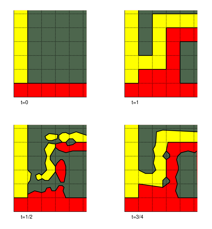
Figure 10: Homotopy for Brouwer function in the plane

• (the main ideas) Recall the role of discrete Brouwer functions in the reductions from End of the line to Nash, as discussed in Section 4. Suppose ${\mathcal{G}}={\mathcal{G}}_{1}$ is associated with a discrete Brouwer function having the kind of structure indicated in Figure 5; the bottom left-hand corner looks roughly like the top right-hand “$t=1$” diagram in Figure 10. Suppose that ${\mathcal{G}}_{0}$ is associated with a DBF in which the line-encoding structure has been stripped out: the top left “$t=0$” diagram in Figure 10.

  Consider the linear homotopy between the corresponding continuous Brouwer functions ${\mathcal{F}}_{0}$ and ${\mathcal{F}}_{1}$; ${\mathcal{F}}_{t}(x)=(1-t){\mathcal{F}}_{0}(x)+{\mathcal{F}}_{1}(x)$. ${\mathcal{F}}_{t}$ colours the square according to the direction of ${\mathcal{F}}_{t}(x)-x$. Figure 10 (the bottom half) shows how these colourings may evolve for intermediate values of $t$. For intermediate values of $t$, in regions where ${\mathcal{F}}_{0}={\mathcal{F}}_{1}$ we have ${\mathcal{F}}_{t}(x)={\mathcal{F}}_{0}(x)={\mathcal{F}}_{1}(x)$ for all $t$. This means that fixpoints of ${\mathcal{F}}_{t}$ cannot be located in the region where ${\mathcal{F}}_{1}$ gets the colour 0 (or black). So, a continuous path of fixpoints necessarily follows the line of non-black regions of ${\mathcal{F}}_{1}$, and necessarily ends up at the end of that particular line. The crossover gadget (Figure 6) would break this correspondence with Oeotl; we fix that by moving to 3-dimensions, where the gadget is not needed.       $\square$

8 From Games to Markets

The PPAD-completeness results for variants of Nash has led, more recently, to PPAD-completeness results for the problems of computing certain types of market equilibria. We continue by giving the general idea and intuition, then we proceed to the formal definitions. For more details on the background to this topic, see Chapters 5,6 of [55]; here we aim to focus on giving a brief overview of more recent PPAD-completeness results.

Suppose we have a set $G$ of goods and a set $T$ of traders. Each trader $i$ in $T$ has a utility function $f^{i}$ that maps bundles of goods to non-negative real values. Assume the goods are divisible, so $f^{i}$ is a mapping from vectors of non-negative numbers (the quantity of each good in a bundle) to non-negative real numbers. A standard assumption is that $f^{i}$ should be continuous, and non-decreasing when restricted to an individual good (it doesn’t hurt to receive a bigger quantity), and concave (there is non-increasing marginal utility). Now, suppose that each good $j$ gets a (non-negative real) unit price $p_{j}$. A trader with some given budget can then identify (from $f^{i}$) the optimal bundle of goods that his budget will purchase (where optimal bundles need not be unique). In general, the aim is to identify prices for goods such that each trader can exchange an initial allocation for an optimal one that has the same total price, so that the total quantity of each good is conserved. Under some fairly mild conditions, it can be shown that such prices always exist. Intuitively, if all traders try to exchange their initial allocations for ones that are optimal, and there is too much demand for good $j$ as a result, then we can fix that problem by raising the price of $j$.

Definition 8.1

In an Arrow-Debreu market [3], each trader has an initial endowment consisting of a bundle of goods. Suppose that the prices are set such that the following can happen: each trader exchanges his endowment for an optimal bundle having the same total value, and furthermore, the total quantity of each good is conserved. In that case, we say that these prices allow the market to clear. It is shown in [3] that there always exist prices that allow the market to clear.

A Fisher market is a special case of an Arrow-Debreu market, in which traders are initially endowed with quantities of money, and there are fixed quantities of goods for sale; in this case the prices should ensure that if each trader buys a bundle of goods that is optimal for his budget, then all goods are sold. This can be seen to be a special case of Arrow-Debreu market, by regarding money as one of the goods in $G$.

The existence proof of market-clearing prices [3] works by expressing a market satisfying the relevant constraints in terms of an abstract economy, a generalisation of the standard notion of a game, and applying Nash’s theorem. So, indirectly the proof uses Brouwer’s fixed point theorem. This indicates that PPAD is the relevant complexity class for studying the hardness of computing a price equilibrium. Results about the computational complexity of finding market-clearing prices are in terms of the types of utility functions of the traders.

Interesting classes of utility functions include the following (where $(x_{1},\ldots,x_{m})$ denotes a vector of quantities of $m$ goods):

1. Additively separable functions, where a trader’s function $f^{i}(x_{1},\ldots,x_{m})$ is of the form $f^{i}(x_{1},\ldots,x_{m})=\sum_{j=1}^{m}f^{i}_{j}(x_{j})$. We still need to specify the structure of the functions $f^{i}_{j}$ in order to have a well-defined problem.

2. piecewise linear: in conjunction with additively separable, this would require that each function $f^{i}_{j}(x_{j})$ be piecewise linear, and the syntactic complexity of such a function would be the total number of pieces of the functions $f^{i}_{j}$. More generally, without the additively separable property, $f^{i}$ could take the form $f^{i}(x_{1},\ldots,x_{m})=\min_{a\in A}f^{i}_{a}(x_{1},\ldots,x_{m})$ where $A$ indexes a finite set of linear functions, and $f^{i}_{a}(x_{1},\ldots,x_{m})=\sum_{j=1}^{m}\lambda^{a}_{j}x_{j}$ for non-negative coefficients $\lambda^{a}_{j}$.

3. Leontiev economies: In a Leontiev economy we have $f^{i}(x_{1},\ldots,x_{m})=\min_{j\in[m]}\lambda^{i}_{j}x_{j}$, a special case of the piecewise linear functions above; note that these functions are not however additively separable.

Polynomial-time algorithms

Linear utility functions take the form $f^{i}(x_{1},\ldots,x_{m})=\sum_{j=1}^{m}\lambda^{i}_{j}x_{j}$ — they are both additively separable and piecewise linear, but not Leontiev; they were initially considered in [34], and are known to be solvable in polynomial time [28, 46] in the case of Fisher markets. For the Arrow-Debreu case, Devanur and Vazirani [29] give a strongly polynomial-time approximation scheme but leave open the problem of finding an exact one in polynomial time.

PPAD-hardness results

The first such result applied to Leontiev economies, for which there is a reduction from 2-player games [17]. Chen et al. [9] show that it is PPAD-complete to compute an Arrow-Debreu market equilibrium for the case of additively separable, piecewise linear and concave utility functions. Chen and Teng [15] show that it is PPAD-hard to compute Fisher equilibrium prices, from utility functions that are additively separable and piecewise linear concave; this is done by reduction from Sparse bimatrix [14]. Vazirani and Yannakakis [66] show that finding an equilibrium in Fisher markets is PPAD-hard in the case of additively-separable, piecewise-linear, concave utility functions. On the positive side, they show that with these utility functions, market equilibria can however be written down with rational numbers.

References

- [1] T.G. Abbott, D.M. Kane and P. Valiant, On the complexity of two-player win-lose games, in 46th Symposium on Foundations of Computer Science IEEE Computer Society, (2005), 113-122.
- [2] L. Addario-Berry, N. Olver and A. Vetta, A polynomial time algorithm for finding Nash equilibria in planar win-lose games, J. Graph Algorithms Appl. 11(1) (2007), 309-319.
- [3] K.J. Arrow and G. Debreu, Existence of an Equilibrium for a Competitive Economy, Econometrica 22(3) (1954), 265-290.
- [4] P. Beame, S. Cook, J. Edmonds, R. Impagliazzo and T. Pitassi, The relative complexity of NP search problems, in 27th ACM Symposium on Theory of Computing (1995), 303-314.
- [5] F. Brandt, F. Fischer, P. Harrenstein and Y. Shoham, Ranking Games, Artificial Intelligence 173(3) (2009), 221-239.
- [6] P. Briest, P.W. Goldberg and H. Röglin, Approximate Equilibria in Games with Few Players, CoRR abs/0804.4524 (2008),
- [7] F.E. Browder, On continuity of fixed points under deformations of continuous mappings, Summa Brasiliensis Math. 4 (1960), 183-191.
- [8] V. Bubelis, On equilibria in finite games, International Journal of Game Theory 8 (1979), 65-79.
- [9] X. Chen, D. Dai, Y. Du and S.-H. Teng, Settling the Complexity of Arrow-Debreu Equilibria in Markets with Additively Separable Utilities, in 50th Symposium on Foundations of Computer Science IEEE Computer Society, (2009), 273-282.
- [10] X. Chen and X. Deng, On the complexity of 2D discrete fixed point problem, in 33rd International Colloquium on Automata, Languages and Programming (2006), 489-500.
- [11] X. Chen and X. Deng, Settling the complexity of 2-player Nash Equilibrium, in 47th Symposium on Foundations of Computer Science IEEE Computer Society, (2006), 261-272.
- [12] X. Chen and X. Deng, 3-NASH is PPAD-Complete, Technical report TR05-134, Electronic Colloquium on Computational Complexity (2005),
- [13] X. Chen, X. Deng and S.-H. Teng, Settling the complexity of computing two-player Nash equilibria, Journal of the ACM 56(3) (2009), 1-57.
- [14] X. Chen, X. Deng and S.-H. Teng, Sparse Games are Hard, in 2nd Workshop on Internet and Network Economics (WINE) (2006), 262-273.
- [15] X. Chen and S.-H. Teng, Spending Is Not Easier Than Trading: On the Computational Equivalence of Fisher and Arrow-Debreu Equilibria, in 20th International Symposium on Algorithms and Computation (2009), 647-656.
- [16] B. Codenotti, M. Leoncini and G. Resta, Efficient computation of Nash equilibria for very sparse win-lose games, in 14th European Symposium on Algorithms (2006), 232-243.
- [17] B. Codenotti, A. Saberi, K. Varadarajan and Y. Ye, Leontief economies encode nonzero sum two-player games, in 17th Annual ACM-SIAM Symposium on Discrete Algorithms (2006), 659-667.
- [18] V. Conitzer and T. Sandholm, Complexity results about Nash equilibria, in 18th International Joint Conference on Arti cial Intelligence (2003), 765-771.
- [19] P. Crescenzi and C.H. Papadimitriou, Reversible Simulation of Space-Bounded Computations, Theoretical Computer Science 143(1) (1995), 159-165.
- [20] C. Daskalakis, A. Fabrikant, C.H. Papadimitriou, The Game World Is Flat: The Complexity of Nash Equilibria in Succinct Games, in 33rd International Colloquium on Automata, Languages and Programming (2006), 513-524.
- [21] C. Daskalakis, P.W. Goldberg and C.H. Papadimitriou, The complexity of computing a Nash equilibrium, in 38th ACM Symposium on Theory of Computing (2006), 71-78.
- [22] C. Daskalakis, P.W. Goldberg and C.H. Papadimitriou, The Complexity of Computing a Nash Equilibrium, SIAM Journal on Computing 39(1) (2009), 195-259.
- [23] C. Daskalakis, P.W. Goldberg and C.H. Papadimitriou, The Complexity of Computing a Nash Equilibrium, Communications of the ACM 52(2) (2009), 89-97.
- [24] C. Daskalakis, A. Mehta and C.H. Papadimitriou, A Note on Approximate Nash Equilibria, Theoretical Computer Science 410(17) (2009), 1581-1588.
- [25] C. Daskalakis and C.H. Papadimitriou, Three-player games are hard, Technical Report TR05-139, Electronic Colloquium on Computational Complexity (2005), 1-10.
- [26] C. Daskalakis and C.H. Papadimitriou, Discretized Multinomial Distributions and Nash Equilibria in Anonymous Games, in 49th Symposium on Foundations of Computer Science IEEE Computer Society, (2008), 25-34.
- [27] C. Daskalakis and C.H. Papadimitriou, On a Network Generalization of the Minmax Theorem, in 36th International Colloquium on Automata, Languages and Programming (2009), 423-434.
- [28] N. Devanur, C.H. Papadimitriou, A. Saberi and V.V. Vazirani, Market Equilibrium via a Primal-Dual-Type Algorithm for a Convex Program, Journal of the ACM 55(5) (2008), 1-18.
- [29] N.R. Devanur and V.V. Vazirani, An improved approximation scheme for computing Arrow-Debreu prices for the linear case, in 23rd Conference, Foundations of Software Technology and Theoretical Computer Science (2003), 149-155.
- [30] E. Elkind, L.A. Goldberg and P.W. Goldberg, Nash Equilibria in Graphical Games on Trees Revisited, in 7th ACM Conference on Electronic Commerce (2006), 100-109.
- [31] K. Etessami and M. Yannakakis, On the Complexity of Nash Equilibria and Other Fixed Points, SIAM Journal on Computing 39(6) (2010), 2531-2597.
- [32] U. Feige and I. Talgam-Cohen, A Direct Reduction from -Player to 2-Player Approximate Nash, in 3rd Symposium on Algorithmic Game Theory Springer LNCS 6386, (2010), 138-149.
- [33] L. Fortnow, R, Impagliazzo, V. Kabinets and C. Umans, On the Complexity of Succinct Zero-Sum Games, in 20th IEEE Conference on Computational Complexity (2005), 323-332.
- [34] D. Gale, Theory of Linear Economic Models, McGraw Hill, NY (1960).
- [35] I. Gilboa and E. Zemel, Nash and correlated equilibria: Some complexity considerations, Games and Economic Behavior 1 (1989), 80-93.
- [36] L.A. Goldberg, P.W. Goldberg, P. Krysta and C. Ventre, Ranking Games that have Competitiveness-based Strategies, in 11th ACM Conference on Electronic Commerce (2010), 335-344.
- [37] P.W. Goldberg and C.H. Papadimitriou, Reducibility Among Equilibrium Problems, in 38th ACM Symposium on Theory of Computing (2006), 61-70.
- [38] P.W. Goldberg, C.H. Papadimitriou and R. Savani, The Complexity of the Homotopy Method, Equilibrium Selection, and Lemke-Howson Solutions, Arxiv technical report 1006.5352 (2010), 1-22.
- [39] J.C. Harsanyi, The tracing procedure: a Bayesian approach to de ning a solution for n-person noncooperative games, International Journal of Game Theory 4 (1975), 61-95.
- [40] S. Hémon, M. de Rougemont and M. Santha, Approximate Nash Equilibria for Multi-player Games, in 1st Symposium on Algorithmic Game Theory (2008), 267-278.
- [41] P.J-J. Herings, Two simple proofs of the feasibility of the linear tracing procedure, Economic Theory 15 (2000), 485-490.
- [42] P.J-J. Herings and A. van den Elzen, Computation of the Nash Equilibrium Selected by the Tracing Procedure in N-Person Games, Games and Economic Behavior 38 (2002), 89-117.
- [43] P.J-J Herings and R.J.A.P. Peeters, A differentiable homotopy to compute Nash equilibria of n-person games, Economic Theory 18(1) (2001), 159-185.
- [44] P.J-J. Herings and R. Peeters, Homotopy methods to compute equilibria in game theory, Economic Theory 42(1) (2010), 119-156.
- [45] M.D. Hirsch, C.H. Papadimitriou and S. Vavasis, Exponential Lower Bounds for Finding Brouwer Fixed Points, Journal of Complexity 5(4) (1989), 379-416.
- [46] K. Jain, A polynomial-time algorithm for computing the Arrow-Debreu market equilibrium for linear utilities, in 45th Symposium on Foundations of Computer Science IEEE Computer Society, (2004), 286-294.
- [47] M. Kearns, M.L. Littman and S. Singh, Graphical models for game theory, in 17th Conference on Uncertainty in Artificial Intelligence Morgan Kaufmann, (2001), 253-260.
- [48] C.E. Lemke and J.T. Howson, Jr., Equilibrium points of bimatrix games, SIAM J. Appl. Math. 12(2) (1964), 413-423.
- [49] R. Lipton, V. Markakis and A. Mehta, Playing Large Games using Simple Strategies, in 4th ACM Conference on Electronic Commerce (2003), 36-41.
- [50] M. Littman, M. Kearns and S. Singh, An efficient, exact algorithm for single connected graphical games, in 15th Annual Conference on Neural Information Processing Systems MIT Press, (2001), 817-823.
- [51] N. Megiddo, A note on the complexity of -matrix LCP and computing an equilibrium, Res. Rep. RJ6439, IBM Almaden Research Center, San Jose. (1988), 1-5.
- [52] D. Monderer and L. Shapley, Potential Games, Games and Economic Behavior 14 (1996), 124-143.
- [53] J. Nash, Noncooperative Games, Annals of Mathematics 54 (1951), 289-295.
- [54] J. von Neumann and O. Morgenstern, The Theory of Games and Economic Behavior, second ed., Princeton University Press, (1947).
- [55] N. Nisan, T. Roughgarden, E. Tardos and V.V. Vazirani, Algorithmic Game Theory, Cambridge University Press, (2007).
- [56] M.J. Osborne and A. Rubinstein, A Course in Game Theory, MIT Press, (1994).
- [57] C.H. Papadimitriou, On the complexity of the parity argument and other inefficient proofs of existence, J. Comput. System Sci. 48 (1994), 498-532.
- [58] J. Renegar, A faster PSPACE algorithm for deciding the existential theory of the reals, in 29th Symposium on Foundations of Computer Science IEEE Computer Society, (1988), 291-295.
- [59] R.W. Rosenthal, A Class of Games Possessing Pure-Strategy Nash Equilibria, International Journal of Game Theory 2 (1973), 65-67.
- [60] J.-J. Rousseau, Discourse on Inequality, (1754).
- [61] R. Savani and B. von Stengel, Hard-to-Solve Bimatrix Games, Econometrica 74(2) (2006), 397-429.
- [62] H. Scarf, The approximation of fixed points of a continuous mapping, SIAM J. Appl. Math. 15 (1967), 1328-1343.
- [63] G. Schoenebeck and S. Vadhan, The Computational Complexity of Nash Equilibria in Concisely Represented Games, in 7th ACM Conference on Electronic Commerce (2006), 270-279.
- [64] E. Sperner, Neuer Beweis für die Invarianz der Dimensionszahl und des Gebietes, Abhandlungen aus dem Mathematischen Seminar Universität Hamburg 6 (1928), 265-272.
- [65] B. von Stengel, Computing equilibria for two-person games. Chapter 45, Handbook of Game Theory, Vol 3, (eds. R.J. Aumann and S. Hart), North-Holland, Amsterdam (2002). 1723-1759.
- [66] V.V. Vazirani and M. Yannakakis, Market Equilibrium under Separable, Piecewise-Linear, Concave Utilities, in 1st Symposium on Innovations in Computer Science (2010), 156-165.