Statistical regularities in the rank-citation profile of scientists

Abstract

Recent “science of science” research shows that scientific impact measures for journals and individual articles have quantifiable regularities across both time and discipline. However, little is known about the scientific impact distribution at the scale of an individual scientist. We analyze the aggregate scientific production and impact of individual careers using the rank-citation profile $c_{i}(r)$ of 200 distinguished professors and 100 assistant professors. For the entire range of paper rank $r$, we fit each $c_{i}(r)$ to a common distribution function that is parameterized by two scaling exponents. Since two scientists with equivalent Hirsch $h$-index can have significantly different $c_{i}(r)$ profiles, our results demonstrate the utility of the $\beta_{i}$ scaling parameter in conjunction with $h_{i}$ for quantifying individual publication impact. We show that the total number of citations $C_{i}$ tallied from a scientist’s $N_{i}$ papers scales as $C_{i}\sim h_{i}^{1+\beta_{i}}$. Such statistical regularities in the input-output patterns of scientists can be used as benchmarks for theoretical models of career progress.

A scientist’s career path is subject to a myriad of decisions and unforeseen events, e.i. Nobel Prize worthy discoveries citationboosts , that can significantly alter an individual’s career trajectory. As a result, the career path can be difficult to analyze since there are potentially many factors (e.g. individual, mentor-apprentice, institutional, coauthorship, field) Matthew1 ; Matthew2 ; socialstratification ; TeamAssembly ; mentoreffect ; UnivCite ; Scientists to account for in the statistical analysis of scientific panel data.

The rank-citation profile, $c_{i}(r)$, represents the number of citations of individual $i$ to his/her paper $r$, ranked in decreasing order $c_{i}(1)\geq c_{i}(2)\geq\dots c_{i}(N)$, and provides a quantitative synopsis of a given scientist’s publication career. Here, we analyze the rank-ordered citation distribution $c_{i}(r)$ for $300$ scientists in order to better understand patterns of success and to characterize scientific production at the individual scale using a common framework. The review of scientific achievement for post-doctoral selection, tenure review, award and academy selection, at all stages of the career is becoming largely based on quantitative publication impact measures. Hence, understanding quantitative patterns in production are important for developing a transparent and unbiased review system. Interestingly, we observe statistical regularities in $c_{i}(r)$ that are remarkably robust despite the idiosyncratic details of scientific achievement and career evolution. Furthermore, empirical regularities in scientific achievement suggest that there are fundamental social forces governing career progress CareerTrajectory ; BB2 ; GrowthDynamicsH ; GrowthCareers .

We group the 300 scientists that we analyze into three sets of $100$, referred to as datasets A, B and C, so that we can analyze and compare the complete publication careers of each individual, as well as across the three groups:

1. 100 highly-profile scientists with average $h$-index $\langle h\rangle=61\pm 21$. These scientists were selected using the citation shares metric Scientists to quantify cumulative career impact in the journal Physical Review Letters (PRL).

2. 100 additional “control” scientists with average $h$-index $\langle h\rangle=44\pm 15$.

3. 100 current Assistant professors with average $h$-index $\langle h\rangle=14\pm 7$. We selected two scientists from each of the top-50 US physics departments (departments ranked according to the magazine U.S. News).

In the methods section we describe the selection procedure for datasets A, B and C in more detail.

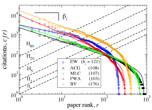
Figure 1: The citation distribution of individual scientists is heavy-tailed. We show 5 empirical rank-citation $c_{i}(r)$ profiles corresponding to extremely high-impact scientists whose initials and $h$-index (as of Jan. 2010) are listed in the legend. The hierarchical scaling pattern in $c_{i}(r)$ for small $r$ values indicate that the pillar contributions of top scientists are “off-the-charts” since they have no characteristic scale. Furthermore, this statistical regularity demonstrates the utility of the $\beta_{i}$ scaling exponent in characterizing the highly cited papers of a given scientist $i$. Interestingly, each scientist has coauthored a significant number of papers that are significantly lower impact than their $c_{i}(1)$ pillar paper. The $c_{i}(r)$ distributions show significant variability in both the high-rank ($\beta$) and low-rank ($\gamma$) regimes. Moreover, for $c_{i}(r)$ with similar $h$ values, the $h$-index (a single point on each curve) is insufficient to adequately distinguish career profiles. The solid curves are the best-fit DGBD functions (see Eq. 3) for each corresponding $c_{i}(r)$ over the entire rank range in each case. The intersection of $c_{i}(r)$ with the line $H_{p}(r)$ corresponds to the generalized $h$-index $h_{p}$, which together uniquely quantify the $c_{i}(r)$ profile. Five $H_{p}(r)$ lines are provided for reference, with $p=\{1,2,5,20,80\}$.

There are many conceivable ways to quantify the impact of a scientist’s $N_{i}$ publications. The $h$-index H is a widely acknowledged single-number measure that serves as a proxy for production and impact simultaneously. The $h$-index $h_{i}$ of scientist $i$ is defined by a single point on the rank-citation profile $c_{i}(r)$ satisfying the condition

$$c_{i}(h_{i})=h_{i}\ .$$ (1)

To address the shortcomings of the $h$-index, numerous remedies have been proposed in the bibliometric sciences ComparisonIndex . For example, Egghe proposed the $g$-index, where the most cited $g$ papers cumulate $g^{2}$ citations overall G , and Zhang proposed the $e$-index which complements the $h$ and $g$ indices quantitatively E .

To justify the importance of analyzing the entire profile $c_{i}(r)$, consider a scientist $i=1$ with rank-citation profile $c_{1}(r)\equiv$ [100, 50, 33, 25, 20, 16, 14, 12, 11, 10, 9…] and a scientist $i=2$ with $c_{2}(r)\equiv$ [10, 10, 10, 10, 10, 10, 10, 10, 10, 10, 9 …]. Both scientists have the same $h$-index value $h=10$, although $c_{1}(r)$ tallies 2.9 times as many citations as $c_{2}(r)$ from his/her most-cited 10 papers. Hence, an additional parameter $\beta_{i}$ is necessary in order to distinguish these two example careers. Specifically, the $\beta_{i}$ parameter quantifies the scaling slope in $c_{i}(r)$ for the high-rank papers corresponding to small $r$ values. In this simple illustration, $\beta_{1}\approx 1$ while $\beta_{2}\approx 0$.

In Fig. 1 we plot $c_{i}(r)$ for 5 extremely high-impact scientists. The individuals EW, ACG, MLC, and PWA are physicists with the largest $h_{i}$ values in our data set; BV is a prolific molecular biologists who we include in this graphical illustration in order to demonstrate the generality of the statistical regularity we find, which likely exists across discipline. To demonstrate how the singe point $c_{i}(h_{i})$ is an arbitrary point along the $c_{i}(r)$ curve, we also plot the lines $H_{p}(r)\equiv p\ r$ for 5 values of $p=\ \{1,2,5,20,80\}$. The value $p\equiv 1$ recovers the $h$-index $h_{1}=h$ proposed by Hirsch. The intersection of any given line $H_{p}(r)$ with $c_{i}(r)$ corresponds to the “generalized $h$-index” $h_{p}$,

$$c(h_{p})=ph_{p}\ ,$$ (2)

proposed in genH and further analyzed in genH2 , with the relation $h_{p}\leq h_{q}$ for $p>q$. Since the value $p\equiv 1$ is chosen somewhat arbitrarily, we take an alternative approach which is to quantify the entire $c_{i}(r)$ profile at once (which is also equivalent to knowing the entire $h_{p}$ spectrum). Surprisingly, because we find regularity in the functional form $c_{i}(r)$ for all 300 scientists analyzed, we can relate the relative impact of a scientist’s publication career using the small set of parameters that specify the $c_{i}(r)$ profile for the entire set of papers ranging from rank $r=1...N_{i}$. Using a much smaller parameter space than the $h_{p}$ spectrum, we can begin to analyze the statistical regularities in the career accomplishments of scientists.

The aim of this analysis is not to add another level of scrutiny to the review of scientific careers, but rather, to highlight the regularities across careers and to seed further exploration into the mechanisms that underlie career success. The aim of this brand of quantitative social science is to utilize the vast amount of information available to develop an academic framework that is sustainable, efficient and fruitful. Young scientific careers are like “startup” companies that need appropriate venture funding to support the career trajectory through lows as well as highs GrowthCareers .

I Results

I.1 A Quantitative Model for $c_{i}(r)$

For each scientist $i$, we find that $c_{i}(r)$ can be approximated by a scaling regime for small $r$ values, followed by a truncated scaling regime for large $r$ values. Recently a novel distribution, the discrete generalized beta distribution (DGBD)

$$c_{i}(r)\equiv A_{i}r^{-\beta_{i}}(N_{i}+1-r)^{\gamma_{i}}$$ (3)

has been proposed as a model for rank profiles in the social and natural sciences that exhibit such truncated scaling behavior DGBfunc ; RankOrder . The parameters $A_{i}$, $\beta_{i}$, $\gamma_{i}$ and $N_{i}$ are each defined for a given $c_{i}(r)$ corresponding to an individual scientists $i$, however we suppress the index $i$ in some equations to keep the notation concise. We estimate the two scaling parameters $\beta_{i}$ and $\gamma_{i}$ using Mathematica software to perform a multiple linear regression of $\ln c_{i}(r)=\ln A_{i}-\beta_{i}\ln r+\gamma_{i}\ln(N_{i}+1-r)$ in the base functions $\ln r$ and $\ln(N_{i}+1-r)$. In our fitting procedure we replace $N$ with $r_{1}$, the largest value of $r$ for which $c(r)\geq 1$ (we find that $r_{1}/N_{i}\approx 0.84\pm 0.01$ for careers in datasets A and B). Figs. 1 and 2 demonstrate the utility of the DGBD to represent $c_{i}(r)$, for both large and small $r$. The regression correlation coefficient $R_{i}>0.97$ for all $\ln c_{i}(r)$ profiles analyzed.

The DGBD proposed in DGBfunc is an improvement over the Zipf law (also called the generalized power-law or Lotka-law EggheLotka ) model and the stretched exponential model H since it reproduces the varying curvature in $c_{i}(r)$ for both small and large $r$. Typically, an exponential cutoff is imposed in the power-law model, and justified as a finite-size effect. The DGBD does not require this assumption, but rather, introduces a second scaling exponent $\gamma_{i}$ which controls the curvature in $c_{i}(r)$ for large $r$ values. The DGBD has been successfully used to model numerous rank-ordering profiles analyzed in DGBfunc ; RankOrder which arise in the natural and socio-economic sciences. The relative values of the $\beta_{i}$ and $\gamma_{i}$ exponents are thought to capture two distinct mechanisms that contribute to the evolution of $c_{i}(r)$ DGBfunc ; RankOrder . Due to the data limitations in this study, we are not able to study the dynamics in $c_{i}(r)$ through time. Each $c_{i}(r)$ is a “snapshot” in time, and so we can only conjecture on the evolution of $c_{i}(r)$ throughout the career. Nevertheless, we believe that there is likely a positive feedback effect between the “heavy-weight” papers and “newborn” papers, whereby the reputation of the “heavy-weight” papers can increase the exposure and impact the perceived significance of “newborn” papers during their infant phase. Moreover, the 2-regime power-law behavior of $c_{i}(r)$ suggests that the reinforcement dynamics can be quantified by the scale-free parameters $\beta$ and $\gamma$.

The $\beta_{i}$ value determines the relative change in the $c_{i}(r)$ values for the high-rank papers, and thus it can be used to further distinguish the careers of two scientists with the same $h$-index. In particular, smaller $\beta$ values characterize flat profiles with relatively low contrast between the high and low-rank regions of any given profile, while larger $\beta$ values indicate a sharper separation between the two regions.

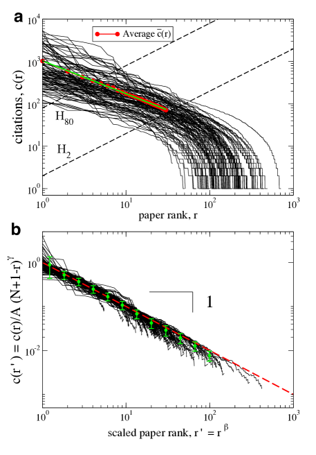
Figure S1: Zipf rank-citation curves plotted in panel (a) correspond to the the 100 dataset [B] scientists. For reference, we plot the average $\overline{c}(r)$ of these 100 curves and find $\overline{c}(r)\sim r^{-\beta}$ with $\beta=0.78\pm 0.01$. The solid green line is a least-squares fit to $\overline{c}(r)$ over the range (a) $1\leq r\leq 30$. We also plot the $H_{p}(r)$ lines corresponding to $p=2$ and $p=80$ for reference. (b) We re-scale the curves in panel (a), plotting $c(r^{\prime})\equiv c(r)/A(N+1-r)^{\gamma}$, where we use the multilinear least-squares regression values for each individual $c_{i}(r)$ profile. Using the rescaled rank value $r^{\prime}\equiv r^{\beta}$, we show excellent data collapse along the expected curve $c(r^{\prime})=1/r^{\prime}$. Green data points correspond to the average $c(r^{\prime})$ value with 1$\sigma$ error bars calculated using all 100 $c_{i}(r^{\prime})$ curves separated into logarithmically spaced bins.

In Fig. 2(a) we plot $c_{i}(r)$ for each scientist from dataset [A] as well as the average of the 100 individual curves $\overline{c}(r)\equiv\frac{1}{100}\sum_{i=1}^{100}c_{i}(r)$ (see Figs. S1 and S2 for analogous plots for datasets [B] and [C]). We find robust power-law scaling

$$\overline{c}(r)\sim r^{-\beta}\ \ \ [\beta\approx 0.92\pm 0.01]$$ (4)

for $10^{0}\leq r\leq 10^{2}$. Interestingly, this $\beta$ value is similar to the scaling exponents calculated for other rank-size (Zipf) distributions in the social and economic sciences, e.g. word frequency ZipfLawWord and city size DGBfunc ; RankOrder ; ZipfLawCity .

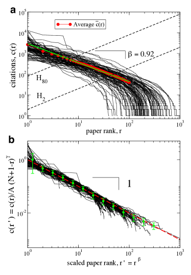
Figure 2: Data collapse of each $c_{i}(r)$ along a universal curve. A comparison of 100 rank-citation profiles $c_{i}(r)$ demonstrates the statistical regularity in career publication output. Each scientist produces a cascade of papers of varying impact between the $c_{i}(1)$ pillar paper down to the least-known paper $c_{i}(N_{i})$. (a) Zipf rank-citation profiles $c_{i}(r)$ for 100 scientists listed in dataset [A]. For reference, we plot the average $\overline{c}(r)$ of these 100 curves and find $\overline{c}(r)\sim r^{-\beta}$ with $\beta=0.92\pm 0.01$. The solid green line is a least-squares fit to $\overline{c}(r)$ over the range $1\leq r\leq 100$. We also plot the $H_{2}(r)$ and $H_{80}(r)$ lines for reference. (b) We re-scale the curves in panel (a), plotting $c_{i}(r^{\prime})\equiv c_{i}(r)/A(r_{1}+1-r)^{\gamma}$, where we use the best-fit $\gamma_{i}$ and $A_{i}$ parameter values for each individual $c_{i}(r)$ profile. Using the rescaled rank value $r^{\prime}\equiv r^{\beta_{i}}$, we show excellent data collapse onto the expected curve $c(r^{\prime})=1/r^{\prime}$. (see Figs. S1 and S2 for analogous plots for dataset [B] and [C] scientists). Green data points correspond to the average $c(r^{\prime})$ value with 1$\sigma$ error bars calculated using all 100 $c_{i}(r^{\prime})$ curves separated into logarithmically spaced bins.

We calculate each $\beta_{i}$ value using a multilinear least-squares regression of $\ln c_{i}(r)$ for $1\leq r\leq r_{1}$ using the DGBD model defined in Eq. [3]. To properly weight the data points for better regression fit over the entire range, we use only $20$ values of $c_{i}(r)$ data points that are equally spaced on the logarithmic scale in the range $r\in[1,r_{1}]$. We elaborate the details of this fitting technique in the methods section. We plot five empirical $c_{i}(r)$ along with their corresponding best-fit DGBD functions in Fig. 1 to demonstrate the goodness of fit for the entire range of $r$.

In order to demonstrate the common functional form of the DGBD model, we collapse each $c_{i}(r)$ along a universal scaling function $c(r^{\prime})=1/r^{\prime}$, by using the rescaled rank values $r^{\prime}\equiv r^{\beta_{i}}$ defined for each curve. In Figs. 2(b), S1(b) and S2(b), we plot the quantity $c_{i}(r^{\prime})\equiv c_{i}(r)/A(r_{1}+1-r)^{\gamma}$, using the best-fit $\gamma_{i}$ and $A_{i}$ parameter values for each individual $c_{i}(r)$ profile. While the curves in Fig. 2(a) are jumbled and distributed over a large range of $c(r)$ values, the rescaled $c_{i}(r)$ curves in Fig. 2(b) all lie approximately along the predicted curve $c(r^{\prime})=1/r^{\prime}$.

I.2 Using $c_{i}(r)$ to quantify career production and impact

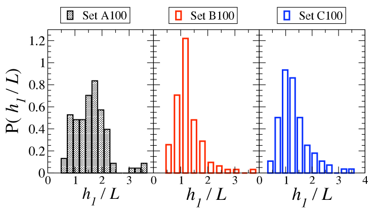
Figure S3: Probability distribution of $h/L$ values calculated for scientists in datasets [A], [B] and [C].

A main advantage of the $h$-index is the simplicity in which it is calculated, e.g. ISI Web of Knowledge WofK readily provides this quantity online for distinct authors. Another strength of the $h$-index is its stable growth with respect to changes in $c_{i}(r)$ due to time and information-dependent factors Hstability . Indeed, the $h$-index is a “fixed-point” of the citation profile. This time stability is evident in the observed growth rates of $h$ for scientists. Average growth rates, calculated here as $h/L$, where $L$ is the duration in years between a given author’s first and most recent paper, typically lie in the range of one to three units per year (this annual growth rate corresponds to the quantity $m$ introduced by Hirsch H ). Annual growth rates $h/L\approx 3$ correspond to exceptional scientists (for the histogram of $P(h/L)$ see the Fig. S3 and for $h/L$ values see the SI text (Tables S1-S4)). As a result, $h/L$ is a good predictor for future achievement along with $h$ H2 .

It is truly remarkable how a single number, $h_{i}$, correlates with other measures of impact. Understandably, being just a single number, the $h$-index cannot fully account for other factors, such as variations in citation standards and coauthorship patterns across discipline hindexResearchers ; hindexFields ; ProConH , nor can $h_{i}$ incorporate the full information contained in the entire $c_{i}(r)$ profile. As a result, it is widely appreciated that the $h$-index can underrate the value of the best-cited papers, since once a paper transitions into the region $r\leq h_{i}$, its citation record is discounted, until other less-cited papers with $r>h_{i}$ eventually overcome the rank “barrier” $r=h_{i}$. Moreover, as noted in H , the papers for which $r>h_{i}$ do not contribute any additional credit.

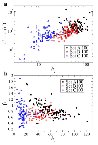
Figure 3: Limitations to the use of the $h$-index alone. The $h$-index can be insufficient in comprehensively representing $c_{i}(r)$. (a) The $h$-index does not contain any information about $c_{i}(r)$ for $r<h_{i}$, and can shield a scientist’s most successful accomplishments which are the basis for much of a scientist’s reputation. This is evident in the cases where $c(r_{i}^{*})\gg h_{i}$, in which case the $h$-index cannot account for the stellar impact of the papers. (b) For a given $h_{i}$ value, prolific careers are characterized by a large $\beta_{i}$ value, as it is harder to maintain large $\beta_{i}$ values for large $h_{i}$. As a result, the $\beta_{i}$ vs $h_{i}$ parameter space can be used to identify anomalous careers and to better compare two scientists with similar $h_{i}$ indices. We find that a third career metric $C_{i}$, the total number of citations to the papers of author $i$, can be calculated with high accuracy by the scaling relation $C_{i}\sim h_{i}^{1+\beta_{i}}$, which we illustrate in Fig. 4(b).

Instead of choosing an arbitrary $h_{p}$ as an productivity-impact indicator, we use the analytic properties of the DGBD to calculate a crossover value $r_{i}^{*}$. In the methods section, we derive an exact expression for $r_{i}^{*}$ which highlights the distinguished papers of a given author. To calculate $r_{i}^{*}$, we use the logarithmic derivative $\chi(r)\equiv d\ln c(r)/dr$ to quantify the relative change in $c_{i}(r)$ with increasing $r$. We defined papers as “distinguished” if they satisfy the inequality $c_{i}(r)/c_{i}(r+1)>\exp(\overline{\chi})$, where $\overline{\chi}$ is the average value of $\chi(r)$ over the entire range of $r$ values. This inequality selects the peak papers which are significantly more cited than their neighbors. The peak region $r\in[1,r_{i}^{*}]$ corresponds to a “knee” in $c_{i}(r)$ when plotted on log-linear axes. The dependence of $\overline{\chi}$ and $r_{i}^{*}$ on the three DGBD parameters $\beta_{i}$, $\gamma_{i}$ and $N_{i}$ are provided in the methods section.

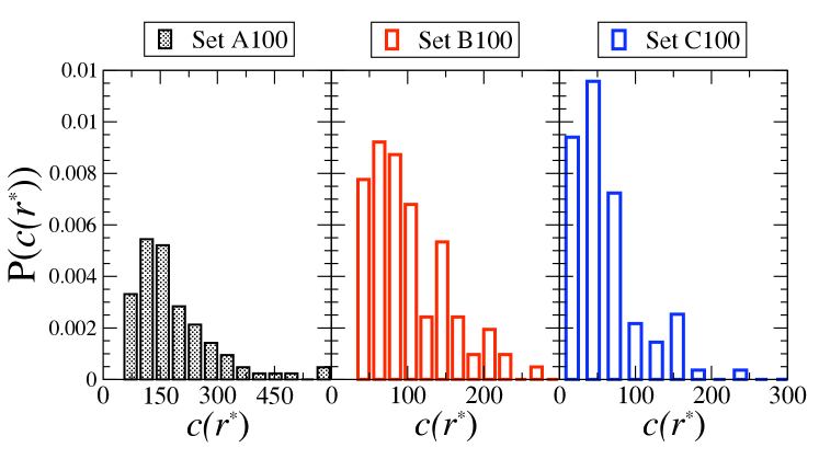
Figure S4: Probability distribution of $c(r^{*})$ values calculated for scientists in datasets [A], [B] and [C].

The advantage of $r_{i}^{*}$ is that this characteristic rank value is a comprehensive representation of the stellar papers in the high-rank scaling regime since it depends on the DGBD parameter values $\beta_{i}$, $\gamma_{i}$ and $N_{i}$, and thus probes the entire citation profile. Fig. 3 shows a scatter plot of the “$c$-star” $c_{i}^{*}\equiv c_{i}(r_{i}^{*})$ and $h_{i}$ values calculated for each scientist and demonstrates that there is a non-trivial relation between these two single-value indices. It also shows that for scientists within a small range of $c^{*}$ there is a large variation in the corresponding $h$ values, in some cases straddling across all three sets of scientists. Also, there are several $c_{i}^{*}$ values which significantly deviate from the trend in Fig. 3, which is plotted on log-log axes. These results reflect the fact that the $h$-index cannot completely incorporate the entire $c_{i}(r)$ profile. We plot the histogram of $c_{i}^{*}$ and $r_{i}^{*}$ values in Figs. S4 and S5, respectively.

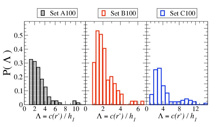
Figure S6: Probability distribution of peak-values $\Lambda\equiv c(r^{*})/h$ for scientists in datasets [A], [B] and [C].

To further contrast the values of $c_{i}^{*}$ and the $h$-index, we propose the “peak indicator” ratio $\Lambda_{i}\equiv c_{i}^{*}/h_{i}$, which corrects specifically for the $h$-index penalty on the stellar papers in the peak region of $c_{i}(r)$. Thus, all papers in the peak region of $c_{i}(r)$ satisfy the condition $c_{i}(r)\geq h_{i}\Lambda_{i}$. In an extreme example, R. P. Feynman has a peak value $\Lambda\approx 36$, indicating that his best papers are monumental pillars with respect to his other papers which contribute to his $h$-index. Fig. S6 shows the histogram of $\Lambda_{i}$ values, with typical values for dataset [A] scientists $\langle\Lambda\rangle\approx 3.4\pm 3.9$, and for dataset [B] scientists $\langle\Lambda\rangle\approx 2.2\pm 1.1$. This indicator can only be used to compare scientists with similar $h$ values, since a small $h_{i}$ can result in a large $\Lambda_{i}$.

An alternative “single number” indicator is $C_{i}$, an author’s total number of citations

$$C_{i}=\sum_{r=1}^{N}c_{i}(r)\ ,$$ (5)

which incorporates the entire $c_{i}(r)$ profile. However, it has been shown that $\sqrt{C_{i}}$ correlates well with $h_{i}$ Hredner , a result which we will demonstrate in Eq. [6] to follow directly from a $c_{i}(r)$ with $\beta_{i}\approx 1$.

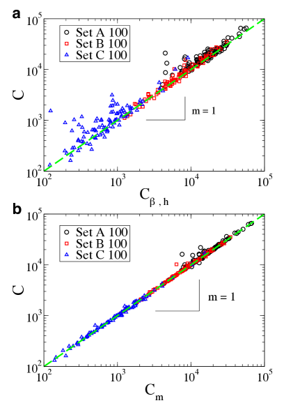
Figure 4: Aggregate publication impact $C$. The total number of citations $C_{i}\sim h_{i}^{1+\beta_{i}}$ is also comprehensive productivity-impact measure. For most best-fit DGBD model curves, the $C_{i}$ value is preserved with high precision. This shows that the difference between a given $c_{i}(r)$ and the corresponding best-fit DGBD model function are negligible on the macroscopic scale. (a) The exact aggregate number of citations $C_{i}$, calculated from $c_{i}(r)$ using Eq. [5], can be analytically approximated by $C_{\beta,h}$ using Eq. [6] which depends only on the scientist’s $\beta_{i}$ and $h_{i}$ values. (b) We justify the use of the DGBD model defined in Eq. [3] for the approximation of $c_{i}(r)$ by comparing the aggregate citations $C_{i}$ with the expected aggregate citations $C_{m}=\sum_{r=1}^{r_{1}}c_{m}(r)$ calculated from the best-fit DGBD model $c_{m}(r)$. Including the extra scaling-parameter, as in the DGBD model, improves the agreement between the theoretical and empirical $C_{i}$ values in (a) and (b). We plot the line $y=x$ (dashed-green line) for visual reference.

We test the aggregate properties of $c_{i}(r)$ by calculating the aggregate number of citations $C_{\beta,h}$ for a given profile,

$$C_{\beta,h}\equiv\sum_{r=1}^{N}Ar^{-\beta}\approx h^{1+\beta}\sum_{r=1}^{N^{\prime}}r^{-\beta}=h^{1+\beta}H_{N^{\prime},\beta}\sim h^{1+\beta}$$ (6)

where $H_{N^{\prime},\beta}$ is the generalized harmonic number and is of order $O(1)$ for $\beta\approx 1$. We neglect the $\gamma_{i}$ scaling regime since the low-rank papers do not significantly contribute to an author’s $C_{i}$ tally. We approximate the coefficient $A$ in Eq. [6] using the definition $c(h)\equiv h$, which implies that $A/h^{\beta}\approx h$. We use the value $N^{\prime}\equiv 3h$, so that $C_{\beta,h}$ can be approximated by only the two parameters $h_{i}$ and $\beta_{i}$ for any given author. We justify this choice of $N^{\prime}$ by examining the rescaled $c_{i}(r/h)$, which we consider to be negligible beyond rank $r=3h_{i}$ for most scientists. In Fig. 4(a), we plot for each scientist the predicted $C_{\beta,h}$ value versus the empirical $C_{i}$ value, and we find excellent agreement with our theoretical prediction $C_{i}\sim h_{i}^{1+\beta_{i}}$ given by Eq. [6]. In Fig. 4(b), we plot for each scientist the total number of citations $C_{m}=\sum_{r=1}^{r_{1}}c_{m}(r)$ using the best-fit DGBD model $c_{m}(r)\equiv c_{i}(r;\beta_{i},\gamma_{i},A_{i},r_{1})$ to approximate $c_{i}(r)$. The excellent agreement demonstrates that the fluctuations in the residual difference $c_{m}(r)-c_{i}(r)$ cancel out on the aggregate level. Furthermore, a comparison of the quality of agreement between the theoretical $C_{i}$ values and the empirical $C_{i}$ values in Fig. 4(a) and (b) shows the importance of the additional $\gamma_{i}$ scaling regime in the DGBD model.

II Discussion

We use the DGBD model to provide an analytic description of $c_{i}(r)$ over the entire range of $r$, and provide a deeper quantitative understanding of scientific impact arising from an author’s career publication works. The DGBD model exhibits scaling behavior for both large and small $r$, where the scaling for small $r$ is quantified by the exponent $\beta_{i}$, which for many scientists analyzed, can be approximated using only two values of the generalized $h$-index $h_{p}$ (see SI text). In particular, we show that for a given $h$-value, a larger $\beta_{i}$ value corresponds to a more prolific publication career, since $C_{i}\sim h_{i}^{1+\beta_{i}}$.

Many studies analyze only the high rank values of generic Zipf ranking profiles $c(r)$, e.g. computing the scaling regime for $r<r_{c}$ below some some rank cutoff $r_{c}$. However, these studies cannot quantitatively relate the large observations to the small observations within the system of interest. To account for this shortcoming, our method for calculating the crossover values $r_{i}^{*}\equiv\overline{r}_{-}$, $r_{\mathsf{x}}$, and $\overline{r}_{+}$, which we elaborate in the methods section, can be used in general to quantitatively distinguish relatively large observations and relatively small observations within the entire set of observations. Moreover, the DGBD model has been shown to have wide application in quantifying the Zipf rank profiles in various phenomena RankOrder .

To measure the upward mobility of a scientist’s career, in the SI text we address the question: given that a scientist has index $h$, what is her/his most likely $h$-index value $\Delta t$ years in the future? In consideration of the bulk of $c_{i}(r)$, and following from the regularity of $c_{i}(r)$ for $r\approx h$, we propose a model-free gap-index $G(\Delta h)$ as both an estimate and a target for future achievement which can be used in the review of career advancement. The gap index $G(\Delta h)$, defined as a proxy for the total number of citations a scientist needs to reach a target value $h+\Delta h$, can detect the potential for fast $h$-index growth by quantifying $c_{i}(r)$ around $h$. This estimator differs from other estimators for the time-dependent $h$-index DynamicH ; StochasticModel ; SimulatingH in that $G(\Delta h)$ is model independent.

Even though the productivity of scientists can vary substantially Scientists ; ShockleyProductivity ; ProductDiff ; huber98 ; PetersonPNAS , and despite the complexity of success in academia, we find remarkable statistical regularity in the functional form of $c_{i}(r)$ for the scientists analyzed here from the physics community. Recent work in Scientists ; UnivCite ; Rad2 calculates the citation distributions of papers from various disciplines and shows that proper normalization of impact measures can allow for comparison across time and discipline. Hence, it is likely that the publication careers of productive scientists in many disciplines obey the statistical regularities observed here for the set of 300 physicists. Towards developing a model for career evolution, it is still unclear how the relative strengths of two contributing factors (i) the extrinsic cumulative advantage effect Matthew1 ; Matthew2 ; Scientists versus (ii) the intrinsic role of the ”sacred spark” in combination with intellectual genius ProductDiff manifest in the parameters of the DGBD model.

With little calculation, the $\beta_{i}$ metric developed here, used in conjunction with the $h_{i}$, can better answer the question, “How popular are your papers?” howpopular . Since the cumulative impact and productivity of individual scientists are also found to obey statistical laws Scientists ; BB2 , it is possible that the competitive nature of scientific advancement can be quantified and utilized in order to monitor career progress. Interestingly, there is strong evidence for a governing mechanism of career progress based on cumulative advantage Scientists ; cumadvprocess ; BB2 coupled with the the inherent talent of an individual, which results in statistical regularities in the career achievements of scientists as well as professional athletes BB0 ; BB2 ; BB3 . Hence, whenever data are available CompSocScience ; SocialDynamicsRev , finding statistical regularities emerging from human endeavors is a first step towards better understand the dynamics of human productivity.

III Methods

III.1 Selection of scientists and data collection

We use disambiguated “distinct author” data from ISI Web of Knowledge. This online database is host to comprehensive data that is well-suited for developing testable models for scientific impact DiffusionRanking ; Scientists ; Rad2 and career progress BB2 . In order to approximately control for discipline-specific publication and citation factors, we analyze 300 scientists from the field of physics.

We aggregate all authors who published in Physical Review Letters (PRL) over the 50-year period 1958-2008 into a common dataset. From this dataset, we rank the scientists using the citations shares metric defined in Scientists . This citation shares metric divides equally the total number of citations a paper receives among the $n$ coauthors, and also normalizes the total number of citations by a time-dependent factor to account for citation variations across time and discipline.

Hence, for each scientist in the PRL database, we calculate a cumulative number of citation shares received from only their PRL publications. This tally serves as a proxy for his/her scientific impact in all journals. The top 100 scientists according to this citation shares metric comprise dataset [A]. As a control, we also choose 100 other dataset [B] scientists, approximately randomly, from our ranked PRL list. The selection criteria for the control dataset [B] group are that an author must have published between 10 and 50 papers in PRL. This likely ensures that the total publication history, in all journals, be on the order of 100 articles for each author selected. We compare the tenured scientists in datasets A and B with 100 relatively young assistant professors in dataset [C]. To select dataset [C] scientists, we chose two assistant professors from the top 50 U.S. physics and astronomy departments (ranked according to the magazine U.S. News).

For privacy reasons, we provide in the SI tables only the abbreviated initials for each scientist’s name (last name initial, first and middle name initial, e.g. L, FM). Upon request we can provide full names.

We downloaded datasets A and B from ISI Web of Science in Jan. 2010 and dataset C from ISI ISI Web of Science in Oct. 2010. We used the “Distinct Author Sets” function provided by ISI in order to increase the likelihood that only papers published by each given author are analyzed. On a case by case basis, we performed further author disambiguation for each author.

III.2 Statistical significance tests for the $c(r)$ DGBD model

We test the statistical significance of the DGBD model fit using the $\chi^{2}$ test between the 3-parameter best-fit DGBD $c_{m}(r)$ and the empirical $c_{i}(r)$. We calculate the $p$-value for the $\chi^{2}$ distribution with $r_{1}-3$ degrees of freedom and find, for each data set, the number $N_{>p_{c}}$ of $c_{i}(r)$ with $p$-value $>p_{c}$: $N_{>p_{c}}$ = 4 [A], 19 [B], 22 [C] for $p_{c}=0.05$, and 8 [A], 22 [B], 37 [C] for $p_{c}=0.01$.

The significant number of $c_{i}(r)$ which do not pass the $\chi^{2}$ test for $p_{c}=0.05$, results from the fact that the DGBD is a scaling function over several orders of magnitude in both $r$ and $c_{i}(r)$ values, and so the residual differences $[c_{i}(r)-c_{m}(r)]$ are not expected to be normally distributed since there is no characteristic scale for scaling functions such as the DGBD. Nevertheless, the fact that so many $c_{i}(r)$ do pass the $\chi^{2}$ test at such a high significance level, provides evidence for the quality-of-fit of the DGBD model. For comparison, none of the $c_{i}(r)$ pass the $\chi^{2}$ test using the power-law model at the $p_{c}=0.05$ significance level. In the next section, we will also compare the macroscopic agreement in the total number of citations for each scientist and the total number of citations predicted by the DGBD model for each scientist, and find excellent agreement. s

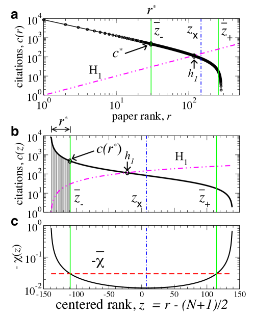
Figure 5: Characteristic properties of the DGBD. We graphically illustrate the derivation of the characteristic $c_{i}(r)$ crossover values that locate the two tail regimes of $c_{i}(r)$, in particular, the distinguished “peak” paper regime corresponding to paper ranks $r\leq r^{*}$ (shaded region). The crossover between two scaling regimes suggests a complex reinforcement relation between the impact of a scientist’s most famous papers and the impact of his/her other papers. (a) The $c_{i}(r)$ plotted on log-log axes with $N=278$, $\beta=0.83$ and $\gamma=0.67$, corresponding to the average values of the Dataset [A] scientists.The hatched magenta curve is the $H_{1}(z)$ line on the log-linear scale with corresponding $h$-index value $h=104$. The $r^{*}$ value for $c_{i}(r)$ is not visibly obvious. (b) We plot on log-linear axes the centered citation profile $c_{i}(z)$ (solid black curve) given by the symmetric rank transformation $z=r-z_{0}$ in Eq. [7]. This representation better highlights the peak paper regime, but fails to highlight the power-law $\beta$ scaling. (c) We plot the corresponding logarithmic derivative $\chi(z)$ of $c(z)$ (solid black curve), which represents the relative change in $c(z)$. The dashed red line corresponds to $-\overline{\chi}$, where $\overline{\chi}$ is the average value of $\chi(z)$ given by Eq. [12]. The values of $\overline{z}_{\pm}$, indicated by the solid vertical green lines, are defined as the intersection of $\overline{\chi}$ with $\chi(z)$ given by Eq. [13]. The regime $z<\overline{z}_{-}$ corresponds to the best papers of a given author. The hatched blue line corresponds to $z_{\mathsf{x}}^{-}$ which marks the crossover between the $\beta$ and $\gamma$ scaling regimes.

III.3 Derivation of the characteristic DGBD $r$ values

Here we use the analytic properties of the DGBD defined in Eq. [3] to calculate the special $r$ values from the parameters $\beta$, $\gamma$ and $N$ which locate the two tail regimes of $c(z)$, and in particular, the distinguished paper regime. The scaling features of the DGBD do not readily convey any characteristic scales which distinguish the two scaling regimes. Instead, we use the properties of $\ln c_{i}(r)$ to characterize the crossover between the high-rank and the low-rank regimes of $c_{i}(r)$.

We begin by considering $c_{i}(r)$ under the centered rank transformation $z=r-z_{0}$, where $z_{0}=(N+1)/2$, then

$$c(z)=A\frac{(z_{0}-z)^{\gamma}}{(z_{0}+z)^{\beta}}\ ,$$ (7)

in the domain $z\in[-(z_{0}-1),(z_{0}-1)]$. The logarithmic derivative of $c(z)$ expresses the relative change in $c(z)$,

$$\chi(z) \equiv \frac{d\ln c(z)}{dz}=\frac{dc(z)/dz}{c(z)}$$ (8)

$$= -\Big{(}\frac{\gamma}{z_{0}-z}+\frac{\beta}{z_{0}+z}\Big{)}=-m\Big{(}\frac{1+\theta x}{1-x^{2}}\Big{)}\ ,$$

where $x=z/z_{0}$, $\theta=\frac{\gamma-\beta}{\gamma+\beta}$, and $m=\Big{(}\frac{\gamma+\beta}{z_{0}}\Big{)}$. The extreme values of $\frac{d\ln c(z)}{dz}$ for $z_{0}\gg 1$ are given by

$$\frac{d\ln c(z)}{dz}\Big{|}_{z=-(z_{0}-1)}\approx-\beta$$ (9)

$$\frac{d\ln c(z)}{dz}\Big{|}_{z=z_{0}-1}\approx-\gamma$$ (10)

and the average value $\overline{\chi}$ is calculated by,

$$\overline{\chi} \equiv \langle\frac{d\ln c(z)}{dz}\rangle$$ (11)

$$= \frac{-m}{(1-1/z_{0})-(1/z_{0}-1)}\int_{-(1-1/z_{0})}^{(1-1/z_{0})}dx\frac{(1+\theta x)}{1-x^{2}}$$

$$= \frac{-m}{2}\ln N$$

The function $\chi(z)$ takes on the value of $\overline{\chi}$ twice at the values $\overline{z}_{\pm}=z_{0}\overline{x}_{\pm}$ corresponding to the solutions to the quadratic equation,

$$\overline{\chi}=-m\Big{(}\frac{1+\theta x}{1-x^{2}}\Big{)}\ ,$$ (12)

which has the solution

$$\overline{x}_{\pm} = -\frac{\theta}{\ln N}\pm\frac{\sqrt{(\ln N)^{2}-2\ln N+\theta^{2}}}{\ln N}$$ (13)

$$\approx -\frac{\theta}{\ln N}\pm\sqrt{1-2/\ln N}$$

for $\theta^{2}/\ln^{2}N\ll 1$. Converting back to rank, then

$$\overline{r}_{\pm}\approx\big{(}\frac{N}{2}\big{)}\big{(}1-\frac{\theta}{\ln N}\pm\sqrt{1-2/\ln N}\big{)}\ ,$$ (14)

and so the value $r^{*}\equiv\overline{r}_{-}$ is the special rank value which distinguishes the set of excellent papers of each given author. The $c$-star value $c_{i}(r^{*})$ is thus a characteristic value arising from the special analytic properties of $c_{i}(r)$. This method for determining the crossover value $r^{*}$ can be applied to any general Zipf profile which can be modeled by the DGBD.

Furthermore, the crossover $z_{\mathsf{x}}$ between the $\beta$ scaling regime and the $\gamma$ scaling regime is calculated from the inflection points of $\ln c(z)$,

$$0=\frac{d^{2}\ln c(z)}{dz^{2}}|_{z=z_{\mathsf{x}}}=\frac{-\gamma}{(z_{0}-z_{\mathsf{x}})^{2}}+\frac{\beta}{(z_{0}+z_{\mathsf{x}})^{2}}$$ (15)

which has 2 solutions $z_{\mathsf{x}}^{\pm}=z_{0}\Big{(}\frac{1\pm\zeta}{1\mp\zeta}\Big{)}$ , where $\zeta\equiv\sqrt{\gamma/\beta}$. Only $|z_{\mathsf{x}}^{-}|<z_{0}$ is a physical solution. Transforming back to rank values, we find $r_{\mathsf{x}}=z_{0}+z_{\mathsf{x}}^{-}=z_{0}\frac{2}{1+\zeta}=\frac{N+1}{1+\zeta}$. We illustrate these special $z$ values in Fig. 5.

IV Acknowledgments

We thank J. E. Hirsch and J. Tenenbaum for helpful suggestions.

I Simple method for estimating the $\beta$ scaling of $c_{i}(r)$ using two $h_{p}$ values

We analyze the citation profiles of 300 prolific scientists who published Physical Review Letters, and find statistical regularity in the functional form of $c_{i}(r)$ of each individual scientist $i$. Here we further quantify $c_{i}(r)$ and discuss the information contained in the “generalized” $h$-index $h_{p}$, defined by the relation:

$$c(h_{p})=ph_{p}\ ,$$ (S1 )

with $p>1$ a positive integer. In analogy to the $h$-index, $h_{p}$ is the number of papers which are cited at least $ph_{p}$ times. By definition, $h/p<h_{p}<h$. Also, the index $h_{p}$ can be viewed as a functional transform in $p-$space of the citation profile $c_{i}(r)$. This transform exhibits a number of characteristic values, namely $h_{1}\equiv h$, the standard $h$ index, $h_{0}=N$, the total number of papers, and $h_{\infty}=c(1)$, a scientist’s top-cited paper. Therefore, by changing $p$ over the entire interval $[0,\infty[$, one gains spectral information of the entire citation profile $c_{i}(r)$ for a given scientist.

Also, for the high-rank power-law regime $c(r)\sim\ r^{-\beta}$, there is a useful relation between $h_{p}$ and $h_{1/p}$. Since $h_{p}=h\ p^{-\mu}$ then the ratio for complementary $p$-values $h_{1/p}/h_{p}=p^{2\mu}$, where $\mu=1/(1+\beta)$. Small values of $\mu\approx 1$ indicate slowly-decaying $c_{i}(r)$ corresponding to productive authors with potentially high mobility of the $h$-index. Hence, if $c_{i}(r)$ is power-law, then the relation

$$I_{p}\equiv\frac{h_{p}h_{1/p}}{h^{2}}=1$$ (S2 )

should hold independent of the value of $\beta$. For all scientists analyzed, we calculate $I_{2}$ and find $I_{2}=0.97\pm 0.07$. This implies that $c_{i}(r)$ obeys a power law around $r=h$. This is visually confirmed by inspecting $c_{i}(r/h)$ in Figs. 2(b), S1(b) and S2(b) for $r/h\approx 1$. Hence, we define two complementary mobility indices as

$$m_{2}\equiv\frac{h_{2}}{h}$$ (S3 )

and

$$m_{1/2}\equiv\frac{h_{1/2}}{h}$$ (S4 )

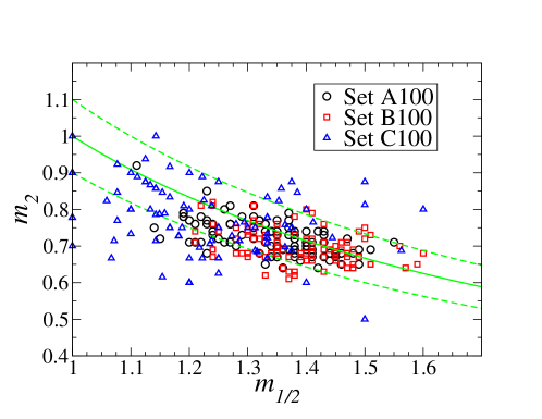
Figure S7: Scatter plot of $m_{1/2}=h_{1/2}/h$ and $m_{2}=h_{2}/h$ for for scientists datasets [A], [B] and [C]. The quantity $I_{2}\equiv m_{1/2}m_{2}\approx 0.97\pm 0.07$ for all scientists analyzed. We plot 3 green curves corresponding to $I_{2}=0.9$, $I_{2}=1.0$, and $I_{2}=1.1$ for comparison.

By definition, $0<m_{2}<1$ and $1<m_{1/2}<N$. The potential for high mobility of the $h$-index is associated with $m_{2}$ close to $1$ (low barrier on the high-cite side) and $m_{1/2}>>1$ (high propensity to change in the low-cite side). We show the relation between $m_{1/2}$ and $m_{2}$ in Fig. S7 along with the expected relation $m_{2}=1/m_{1/2}$ for visual reference.

To test the small-$r$ scaling for each $c_{i}(r)$, we estimate $\beta$ using two methods:

(i) We define an approximation to $\beta$ by assuming $c(r)\sim\ r^{-\beta_{pq}}$ for $r<h$. Hence, two intersection values, $h_{p}$ and $h_{q}$ are sufficient to calculate $\beta_{pq}$ using the relationship for power-law $c_{i}(r)$,

$$\beta_{pq}=\frac{\ln(q/p)}{\ln(h_{p}/h_{q})}-1\ .$$ (S5 )

We use the values $p\equiv 80$ and $q\equiv 2$ since these values generally enclose the scaling regime in the $c_{i}(r)$ profiles (see Fig. 2).

(ii) We calculate $\beta$ using a multilinear least-squares regression of $\ln c_{i}(r)$ for $1\leq r\leq r_{1}$ using the DGBD model defined in Eq. [3]. To properly weight the data points for better regression fit over the entire range, we use only $20$ values of $c_{i}(r)$ data points that are equally spaced on the logarithmic scale in the range $r\in[1,r_{1}]$. We plot four empirical $c_{i}(r)$ along with their corresponding best-fit DGBD functions in Fig. 1 to demonstrate the goodness of fit for the entire range of $r$.

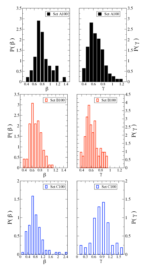
Figure S8: Probability distribution of $\beta$ and $\gamma$ values calculated using multilinear least-squares regression of $\ln c_{i}(r)\equiv\ln A-\beta\ln r+\gamma\ln[r_{1}+1-r]$ for scientists in datasets [A], [B] and [C].

We compare $\beta_{pq}$ and $\beta$ values calculated using methods (i) and (ii) in Tables S1 -S6 and find good agreement. Furthermore, the average scaling exponent $\langle\beta\rangle$ is approximately equal to the value of $\overline{\beta}$ calculated for the average $\overline{c}(r)$ profile in Fig. 2. For the scientists analyzed in dataset [A] we find $\langle\beta\rangle=0.83\pm 0.24$ as compared to $\overline{\beta}=0.92\pm 0.01$. For the scientists analyzed in dataset [B] we find $\langle\beta\rangle=0.70\pm 0.17$ as compared to $\overline{\beta}=0.78\pm 0.01$. We plot the histograms of $\beta$ and $\gamma$ for datasets [A], [B], and [C] in Fig. S8.

II Decomposing the Hirsch $a$ factor to better understand efficiency

Many alternative single-value indicators have been proposed to address the various criticisms of the $h$-index. The $g$-index G differs from the $h$-index in that it lends more weight to the more highly-cited papers. However, as with the $h$-index, the $g$-index does not immediately convey much more information than the total number of citations or the productivity coefficient $a=C/h^{2}$ introduced by Hirsch. In Fig. S9 we plot the histogram of both $h$ and $a$ values for dataset [A] with $\langle a\rangle=6.0\pm 4.1$ and for dataset [B] with $\langle a\rangle=4.2\pm 1.3$, indicating that most researchers do not fall into the ‘step-function’ pathology $\beta\approx 0$ of scientist $2$ above for which $a\approx 1$. Instead, most scientists have a significant number of citations arising from both their high-cited ($r<h$) and low-cited ($r>h$) regions of $c_{i}(r)$.

An interesting decomposition is to write $a$ as the product of two factors,

$$a=\Big{(}\frac{N}{h}\Big{)}\Big{(}\frac{\langle c\rangle}{h}\Big{)}\ ,$$ (S6 )

where $\langle c\rangle\equiv C/N$.

(i) The first factor, by definition, is always greater than $1$, and represents the number of papers in units of $h$. Small values of $N/h$ correspond to scientists who are very efficient (or less productive), while large values correspond to scientists who are very productive (or less efficient). Highly productive authors, who may have a substantial number of papers without a single citation, nevertheless can still have a large $h$-index.

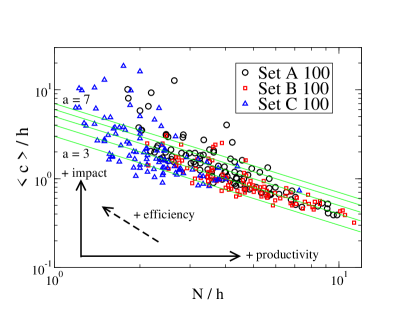
Figure S10: Statistical regularities in the impact-productivity space of scientists. Scatter plot of $N$ and $\langle c\rangle$, in units of $h$, for the 300 scientists analyzed. The quantity $\langle c\rangle$ represents the impact per paper, while the quantity $N/h$ is inversely related to efficiency, since small values correspond to scientists with many citations arising from a relatively small number of papers. Because each quantity is measured in units of $h$, only individuals with similar $h$ can be compared. Dotted green lines correspond to hyperbolic curves hyperbolic curves $\langle c\rangle/h=a/(N/h)$ with values $a=\{3,4,5,6,7\}$ (bottom to top).

(ii) The second factor is the average number of citations per paper $\langle c\rangle$ in units of $h$. Relatively large values of $\langle c\rangle/h>1$ signal the presence of outstanding highly cited papers, i.e. papers with $c(r)\gg h$. Many brilliant careers result from a combination of moderate $N/h\approx 3$ and $\langle c\rangle/h>1$. Fig. S10, which plots $N/h$ versus $\langle c\rangle/h$ for the set of authors examined in this paper, shows a tendency for the two factors to occupy a narrow band of hyperbolic curves $\langle c\rangle/h=a/(N/h)$ with $a\in\{3,7\}$.

III Mobility of the h-index

The $h$-index is taken seriously by many research organizations, affecting important decisions such as tenure, promotions, honors. For instance, Hirsch noted that $h\sim 12$ seems to be appropriate for associate professor, $h\sim 18$ might be suitable for advancement to full professor, while $h\sim 45$ is the average for NAS election H . However, little work has been done to measure the “upward mobility” of the $h$-index with time. Here we address the question: given that a scientist has index $h$, what is her/his most likely $h$-index value $\Delta t$ years in the future? This question is fundamentally related to the growth rate of $c_{i}(r)$ for $r\gtrsim h$. For productive scientists, Hirsch noted that $h$ grows at a rate of about one unit a year H . However, a single-value indicator such as $h$ cannot quantify the probability of “growth spurts”, which should also enter into evaluation criteria (based on the $h$-index, citation counts, etc.).

As a measure of upward mobility, we propose the gap index $G(\Delta h)$, defined as a proxy for the total number of citations a scientist needs to reach a target value $h+\Delta h$, which is similar to the $w(q)$-index proposed in genH2 . The merit of $G(\Delta h)$ is to detect the potential for fast growth by quantifying $c_{i}(r)$ around $h$. For $c_{i}(r)$ with index value $h$ at time $t$, we define $G(\Delta h)$ as the minimum number of citations, distributed to papers $r=\{1,...h+\Delta h\}$, so that the $h$-index value at time $t+\Delta t$ becomes $h+\Delta h$.

Consider the citation gap $g(r)=h^{+}-c(r)$ of each paper $r$ with $c(r)<h^{+}$. Then $G(\Delta h)$ is given by the exact relation which can be easily verified graphically,

$$G(\Delta h)\equiv\sum_{r=h^{-}}^{h^{+}}g(r)=h^{+}(h^{+}-h^{-}+1)-C(h^{-},h^{+})\ ,$$ (S7 )

where $h^{+}=h+\Delta h$, $h^{-}$ is the smallest $r$ value for which $c(r)<h^{+}$, and $C(m,n)=\sum_{r=m}^{n}c(r)$ is the number of citations from paper $m$ up to paper $n$. Hence, $G(\Delta h)$ quantifies the minimum number of citations, assuming perfect assignment, required to bring papers $r=h^{-}\dots h\dots h^{+}$ up to citation level $h^{+}$.

The gap index $G(\Delta h)$ establishes a characteristic time scale $\Delta t$ for the dynamics of $h(t)$. The estimated amount of time for the transition is $\Delta t=Max\{t_{r}\equiv g(r)/\dot{c}(r)\}$ for $h^{-}\leq r\leq h^{+}$, where $\dot{c}(r)$ is its average citation rate (citations/year). This estimate does not take into account ‘rampant papers’, papers with relatively large $r$ and $\dot{c}(r)$, which are either new or rejuvenated after a lengthy period with very few citations 110PhsRev . In practical terms, the short-term utility of $G(\Delta h)$ is for moderate values of $\Delta h$, say in multiples of $5$ or $10$. In other words, for a scientist with $h=12$, a plausible target could be $h^{+}=17$ and a longer term target $h^{+}=22$.

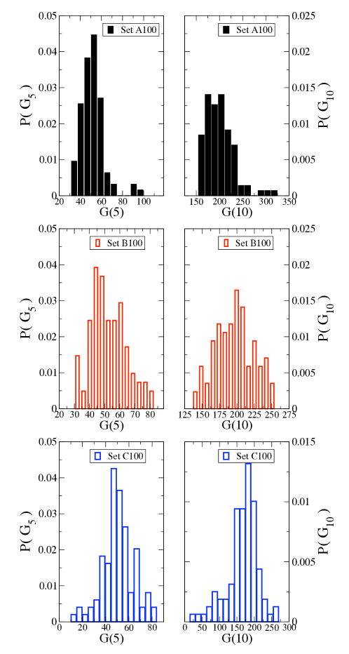
Figure S11: Probability distribution of $G(5)$ and $G(10)$ values calculated for scientists datasets [A], [B] and [C].

In Fig. S11 we plot the histograms for $G(5)$ and $G(10)$. The common distributions between authors in dataset [A] and dataset [B] indicate that the growth potential of $h$ does not depend very strongly on prestige, but rather on the publication patterns of individual authors. Indeed, the average annual growth rate $h/L$ are larger for dataset [A] physicists than dataset [B] physicists, with a significant number of exceptional “outliers” with $h/L>3$.

For young careers corresponding to small $h$-values, there will be a correlation between $G(\Delta h)$ and $h$ because most new citations will contribute to the increase of $h$. However, for an advanced career, not all incoming citations will contribute to an increase in $h$. Hence, to test the dependence of $G(\Delta h)$ on $h$, we perform a linear regression $G_{i}(\Delta h)=g_{0}+g_{1}h_{i}$ for both datasets [A] and [B] and for $\Delta h=5,10$. In each of the four regressions we calculate correlation values $R^{2}<0.05$ and ANOVA (analysis of variance) F-statistics $F<2.3$ for each case, indicating that we accept the null hypothesis that the linear regression coefficient $g_{1}=0$. Thus, for significantly large $h$, the gap-index $G(\Delta h)$ is not dependent on $h$. A similar regression analysis between $G(\Delta h)$ and $\beta$ results in the same conclusion, that the gap index $G(\Delta h)$ is not dependent on $\beta$ for profiles with sufficiently large $h$. Hence, the gap index can be used to estimate the mobility of $h$ and as a comparison index between $c_{i}(r)$.

IV Characterizing the rank-citation $c_{i}(r)$ profile

As many previous studies have shown, and further demonstrated here, there are many conceivable ways to quantify $c_{i}(r)$. In Tables S1-S4 we list $16$ values derived from $c_{i}(r)$ which can serve as quantitative indicators of a scientific career:

1. the author’s total number of papers $N$,

2. the author’s total number of citations $C\equiv\sum_{r=1}^{N}c(r)$,

3. the author’s most-cited paper $c_{i}(1)$,

4. the author’s $c$-star paper $c(r^{*})$, which distinguishes the minimum citation tally of his/her stellar papers in the range $r\in[1,r^{*}]$.

5. the author’s $r^{*}$ value calculated from his/her DGBD parameter values according to Eq. [14]

6. the author’s original $h$-index $h_{1}\equiv h$ and the generalized $h$-index $h_{p}$ for $p=2,80$,

7. the author’s scaling exponent $\beta_{pq}$ calculated using the values $p=2$ and $q=80$ corresponding to $h_{2}$ and $h_{80}$,

8. the author’s scaling exponents $\beta$ and $\gamma$ calculated using multilinear least-squares regression fit to the DGBD model $c_{i}(r)$ in Eq. [3],

9. the author’s peak-value $\Lambda$ given by the $c$-star value $c^{*}$ in units of the $h$-index, $\Lambda\equiv c(r^{*})/h$

10. the author’s number of papers in units of the $h$-index $N^{\prime}\equiv N/h$,

11. the author’s average number of citations per paper in units of the $h$-index $\langle c\rangle^{\prime}\equiv\langle c\rangle/h$,

12. the author’s “productivity” value proposed by Hirsch, $a\equiv C/h^{2}$,

13. the author’s mobility estimator $G(\Delta h)$ quantifying the minimum number of citations needed to increase an individual’s h-value by $\Delta h$ units for $\Delta h=5$ and $\Delta h=10$,

14. the author’s mobility indices $m_{1/2}$ and $m_{2}$ where $m_{1/2}m_{2}\approx 1$,

15. the author’s peak number $P=\frac{1}{h^{2}}\sum_{r=1}^{h}c(r)$,

16. the author’s average $h$-index growth rate $h/L$ over the $L$-year time period between an author’s first and most recent paper.

The $h$-index conveys a very informative one-number picture of productivity, however it does not tell the whole story, since it does not fully capture the impact an author’s most cited papers. Instead, we show the utility of the $c$-star value $c(r^{*})$, which is a better representative of an author’s most cited papers. Thus, we introduce the peak-value indicator $\Lambda\equiv c(r^{*})/h$ in order to characterize the most distinguished papers ($1\leq r\leq r^{*}$) of each given author. The probability distribution of $\Lambda$ values is given in Fig. PeakPDF.

We use the Discrete Generalized Beta Distribution (DGBD) to quantify $c_{i}(r)$ for the whole range of $r$. However, typically a scientist is mostly evaluated by his/her highest ranked papers, say for $r\leq r^{*}$. Hence, in this regime, we show that $c_{i}(r)$ can be parameterized by only two variables, $\beta$ and $h_{1}$, in order to comprehensively capture a publication career. The emergence of a such a compact (two-parameter) and general parametrization highlights an amazing statistical regularity in the scientific productivity of single individuals. Without endorsing the extreme viewpoint ”you are what you publish” or “publish or perish”, such statistical regularity, nevertheless, highlights an outstanding question on the role of social factors in ironing out individual details of human productivity. We believe that such question bears a great relevance to most fields of economic, natural and social sciences, where productivity data are available.

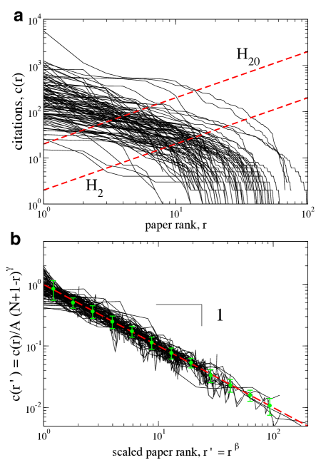
Figure S2: Zipf rank-citation curves plotted in panel (a) correspond to the the 100 dataset [C] assistant professor scientists. For reference, we plot the $H_{p}(r)$ lines corresponding to $p=1$.. (b) We re-scale the curves in panel (a), plotting $c(r^{\prime})\equiv c(r)/A(N+1-r)^{\gamma}$, where we use the multilinear least-squares regression values for each individual $c_{i}(r)$ profile. Using the rescaled rank value $r^{\prime}\equiv r^{\beta}$, we show excellent data collapse along the expected curve $c(r^{\prime})=1/r^{\prime}$ even for young careers. Green data points correspond to the average $c(r^{\prime})$ value with 1$\sigma$ error bars calculated using all 100 $c_{i}(r^{\prime})$ curves separated into logarithmically spaced bins. We note that young careers might possibly be analogous to advanced careers in other disciplines where overall publication rates are lower.

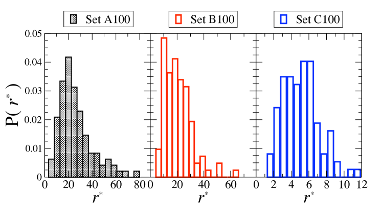
Figure S5: Probability distribution of $r^{*}$ for scientists in datasets [A], [B] and [C].

Figure S9: Probability distribution of $h$ and $a$ values calculated for scientists in datasets [A], [B] and [C].

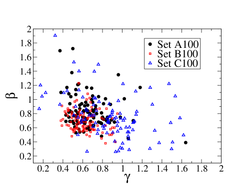
Figure S12: Scatter plot of best-fit $\beta$ and $\gamma$ values.

Name	$N$	$C$	$c(1)$	$c(r^{*})$	$r^{*}$	$h_{1}$	$h_{2}$	$h_{80}$	$\beta_{xy}$	$\beta$	$\gamma$	$c(r^{*})/h_{1}$	$N/h_{1}$	$\langle c\rangle/h_{1}$	$a$	Gap(5)	Gap(10)	$m_{1/2}$	$m_{2}$	$P$	$h_{1}/L$
A, E	116	13848	3339	145	16	41	30	6	1.29	1.17	0.64	3.55	2.83	2.91	8.24	37	165	1.37	0.73	7.67	0.71
A, I	205	15073	783	181	18.3	57	45	6	0.83	0.68	0.76	3.19	3.6	1.29	4.64	44	168	1.37	0.79	3.84	1.9
A, A	363	14996	708	92	33.9	63	44	4	0.54	0.66	0.55	1.46	5.76	0.66	3.78	51	206	1.4	0.7	2.49	1.58
A, BJ	185	18658	6267	133	22.1	51	38	7	1.18	0.94	0.59	2.63	3.63	1.98	7.17	45	176	1.37	0.75	6.25	0.86
A, PW	344	65575	4661	379	32.5	103	78	13	1.06	0.91	0.73	3.69	3.34	1.85	6.18	66	228	1.27	0.76	5.6	1.72
A, A	111	12514	1689	306	9.9	48	38	6	1	0.75	0.98	6.38	2.31	2.35	5.43	71	257	1.19	0.79	5.14	0.81
B, P	173	16709	3037	154	20.9	53	39	5	0.8	0.96	0.63	2.91	3.26	1.82	5.95	57	207	1.34	0.74	5.23	1.61
B, J	141	25350	5636	305	16.1	57	44	9	1.32	0.94	0.81	5.36	2.47	3.15	7.8	55	190	1.32	0.77	7.32	1.08
B, CP	60	10960	2486	264	8.3	28	21	6	1.94	1.35	0.96	9.45	2.14	6.52	14	73	262	1.14	0.75	13.8	0.58
B, CWJ	265	14474	1835	101	28.4	58	39	4	0.62	0.8	0.55	1.75	4.57	0.94	4.3	47	182	1.38	0.67	3.22	2.07
B, CH	78	17715	3849	400	9.8	39	33	8	1.6	1.01	1.02	10.3	2	5.82	11.6	66	229	1.23	0.85	11.3	0.95
B, G	91	15707	6280	240	11.5	46	33	5	0.95	1.01	0.83	5.24	1.98	3.75	7.42	89	292	1.15	0.72	7.17	1.28
B, K	190	21887	12906	82	23.8	45	31	5	1.02	1.17	0.44	1.84	4.22	2.56	10.8	46	186	1.38	0.69	9.94	1.1
B, M	218	16279	1445	148	22.7	55	39	6	0.97	0.84	0.65	2.7	3.96	1.36	5.38	48	203	1.4	0.71	4.49	1.67
C, N	140	9022	2261	117	15.4	43	32	3	0.56	0.77	0.69	2.74	3.26	1.5	4.88	38	168	1.4	0.74	4.11	0.86
C, R	267	18716	5147	128	25.1	66	49	4	0.47	0.74	0.62	1.95	4.05	1.06	4.3	52	214	1.33	0.74	3.51	1.83
C, DM	162	16307	6264	136	19.4	52	36	5	0.87	0.91	0.62	2.62	3.12	1.94	6.03	52	187	1.38	0.69	5.27	1.53
C, DJ	194	13801	1572	166	18.2	56	39	5	0.8	0.74	0.71	2.98	3.46	1.27	4.4	54	210	1.34	0.7	3.64	1.44
C, SW	469	25808	1444	115	44.4	82	56	6	0.65	0.77	0.53	1.4	5.72	0.67	3.84	50	197	1.32	0.68	2.78	3.57
C, JI	295	19894	1514	136	30.4	71	50	6	0.74	0.75	0.6	1.93	4.15	0.95	3.95	58	205	1.38	0.7	3	3.38
C, ML	752	50269	1588	153	63.8	107	69	9	0.81	0.7	0.54	1.44	7.03	0.62	4.39	40	193	1.42	0.64	2.79	1.73
C, PB	220	14257	1878	125	23.4	55	37	5	0.84	0.84	0.61	2.29	4	1.18	4.71	50	174	1.45	0.67	3.75	1.53
D, S	594	19992	2119	65	57.6	65	44	4	0.54	0.69	0.43	1	9.14	0.52	4.73	46	191	1.46	0.68	2.54	1.71
D, SD	108	8339	744	189	10.8	45	33	4	0.75	0.67	0.87	4.22	2.4	1.72	4.12	60	221	1.29	0.73	3.63	0.87
E, DE	235	13741	780	170	15.9	65	44	4	0.54	0.48	0.79	2.63	3.62	0.9	3.25	49	217	1.38	0.68	2.47	1.71
E, JH	347	15475	891	109	29.6	65	45	4	0.52	0.7	0.59	1.68	5.34	0.69	3.66	47	197	1.37	0.69	2.66	1.41
E, VJ	129	11496	1630	194	13.8	46	34	5	0.92	0.81	0.79	4.24	2.8	1.94	5.43	37	160	1.35	0.74	4.81	0.88
E, M	58	16166	12906	55	11.9	22	17	3	1.13	1.69	0.37	2.51	2.64	12.7	33.4	51	199	1.23	0.77	32.9	1.22
F, RP	69	21058	1715	1288	3.8	38	35	9	1.72	0.39	1.64	33.9	1.82	8.03	14.6	100	325	1.11	0.92	14.5	0.76
F, ME	362	33076	1490	231	29.5	93	66	8	0.75	0.63	0.71	2.49	3.89	0.98	3.82	56	216	1.33	0.71	2.94	1.79
F, MPA	145	16913	2260	190	18.1	59	42	7	1.06	0.96	0.7	3.23	2.46	1.98	4.86	74	238	1.2	0.71	4.44	2.11
F, DS	137	16532	1834	275	14	61	43	6	0.87	0.72	0.85	4.51	2.25	1.98	4.44	46	189	1.28	0.7	3.96	1.97
G, H	193	23540	2425	241	20.7	77	52	7	0.84	0.8	0.74	3.14	2.51	1.58	3.97	59	245	1.23	0.68	3.53	2.03
G, C	128	19273	6250	197	16.4	51	40	5	0.77	1.05	0.7	3.88	2.51	2.95	7.41	47	189	1.29	0.78	6.93	1.55
G, SL	157	20303	2548	203	19.4	61	44	6	0.85	1	0.69	3.33	2.57	2.12	5.46	45	202	1.25	0.72	5	1.2
G, AC	1064	44312	1602	103	80.1	108	71	6	0.49	0.69	0.47	0.96	9.85	0.39	3.8	58	243	1.39	0.66	2.31	2.12
G, DJ	217	24264	1722	300	17.3	67	51	8	0.99	0.75	0.85	4.49	3.24	1.67	5.41	36	171	1.33	0.76	4.86	1.52
H, FDM	89	13658	1823	274	11.8	44	34	6	1.13	0.93	0.88	6.25	2.02	3.49	7.05	40	177	1.32	0.77	6.58	1.29
H, BI	272	32647	2978	241	26.9	78	59	10	1.08	0.84	0.7	3.1	3.49	1.54	5.37	48	201	1.27	0.76	4.71	1.73
H, DR	200	18673	2482	210	19.1	64	46	5	0.66	0.83	0.71	3.3	3.13	1.46	4.56	46	173	1.31	0.72	3.92	1.31
H, TW	398	21854	1889	125	35.1	70	50	5	0.6	0.69	0.59	1.79	5.69	0.78	4.46	51	179	1.43	0.71	3.17	1.59
H, H	78	4287	535	121	9	33	25	3	0.74	0.7	0.84	3.69	2.36	1.67	3.94	54	221	1.21	0.76	3.49	1.18
H, SE	200	13256	1423	157	18.7	56	40	5	0.77	0.78	0.69	2.8	3.57	1.18	4.23	47	195	1.27	0.71	3.55	1.19
H, JE	186	10380	535	128	18.2	52	38	4	0.64	0.63	0.7	2.47	3.58	1.07	3.84	44	177	1.38	0.73	2.95	1.53
I, F	249	14235	1231	131	22.7	52	36	6	1.06	0.85	0.64	2.52	4.79	1.1	5.26	55	198	1.38	0.69	4.42	1.13
I, Y	241	12384	1598	102	24.6	52	38	4	0.64	0.87	0.57	1.96	4.63	0.99	4.58	36	163	1.38	0.73	3.66	1.16
J, R	229	26017	1742	286	19.9	74	58	8	0.86	0.75	0.8	3.87	3.09	1.54	4.75	46	188	1.22	0.78	4.21	1.72
J, S	185	12356	3836	75	25.1	43	33	5	0.95	1.04	0.48	1.76	4.3	1.55	6.68	39	172	1.37	0.77	5.74	0.98
K, HJ	241	16011	1228	215	16.7	62	48	6	0.77	0.66	0.79	3.48	3.89	1.07	4.17	45	166	1.35	0.77	3.49	1.68
K, G	211	11298	1949	89	25.1	47	34	4	0.72	0.81	0.55	1.9	4.49	1.14	5.11	34	154	1.47	0.72	3.84	1.57
$\langle x\rangle$	275	20368	2686	183	26	61	44	6	0.85	0.83	0.67	3.37	4.23	1.88	6.04	51	201	1.34	0.72	5.18	1.58
$\sigma$	190	11381	2436	158	14.4	20	14	2	0.31	0.23	0.19	3.87	1.9	2	4.09	11	30	0.09	0.05	4.27	0.59

Table S1: Career citation statistics for 100 dataset [A] scientists: 1-50.

Name	$N$	$C$	$c(1)$	$c(r^{*})$	$r^{*}$	$h_{1}$	$h_{2}$	$h_{80}$	$\beta_{xy}$	$\beta$	$\gamma$	$c(r^{*})/h_{1}$	$N/h_{1}$	$\langle c\rangle/h_{1}$	$a$	Gap(5)	Gap(10)	$m_{1/2}$	$m_{2}$	$P$	$h_{1}/L$
L, RB	79	7751	2271	147	10.8	32	24	5	1.35	1.04	0.76	4.62	2.47	3.07	7.57	43	190	1.31	0.75	7.06	1.07
L, PA	344	32668	3228	208	30.8	80	59	9	0.96	0.8	0.67	2.61	4.3	1.19	5.1	40	166	1.38	0.74	4.26	1.82
L, EH	234	20139	1862	167	25.1	62	46	6	0.81	0.82	0.65	2.7	3.77	1.39	5.24	57	197	1.42	0.74	4.29	1.19
L, SG	379	27530	1355	160	34.9	84	62	6	0.58	0.66	0.62	1.91	4.51	0.86	3.9	53	177	1.43	0.74	2.74	2.33
L, MD	151	11231	876	178	14.5	50	37	5	0.84	0.73	0.8	3.58	3.02	1.49	4.49	50	211	1.24	0.74	3.97	3.13
M, AH	455	17708	641	93	37.9	67	46	4	0.51	0.58	0.56	1.4	6.79	0.58	3.94	43	175	1.49	0.69	2.34	1.91
M, ND	216	10409	2741	83	20.5	41	29	5	1.1	1.07	0.53	2.03	5.27	1.18	6.19	62	216	1.22	0.71	5.52	0.8
M, RN	371	18413	1919	87	40.6	62	42	5	0.73	0.84	0.47	1.41	5.98	0.8	4.79	36	173	1.48	0.68	3.29	1.77
N, DR	191	21742	1371	265	18.3	73	52	8	0.97	0.72	0.81	3.63	2.62	1.56	4.08	57	215	1.26	0.71	3.62	2.09
O, E	438	22310	2973	101	41.6	76	49	5	0.62	0.77	0.51	1.34	5.76	0.67	3.86	43	199	1.36	0.64	2.75	1.85
O, SR	146	5051	1236	59	14.8	26	21	3	0.9	1.14	0.53	2.31	5.62	1.33	7.47	55	183	1.31	0.81	6.7	0.65
P, G	529	29994	2768	108	51.1	81	55	7	0.79	0.82	0.49	1.34	6.53	0.7	4.57	53	194	1.41	0.68	3.23	1.84
P, SSP	330	19184	1760	108	34.7	58	41	7	1.09	0.84	0.53	1.87	5.69	1	5.7	40	157	1.55	0.71	4.18	2
P, M	435	29719	5147	123	43.6	85	57	5	0.52	0.76	0.53	1.45	5.12	0.8	4.11	48	196	1.41	0.67	2.94	2.36
P, JB	298	26621	2719	170	31.5	75	48	7	0.92	0.83	0.61	2.27	3.97	1.19	4.73	54	218	1.36	0.64	3.77	1.79
P, JP	250	62338	12906	173	31.4	62	46	9	1.26	1.38	0.49	2.8	4.03	4.02	16.2	63	224	1.34	0.74	15.4	1.63
P, A	169	10053	3849	50	25.9	37	25	3	0.74	1.1	0.38	1.37	4.57	1.61	7.34	57	203	1.46	0.68	6.23	0.79
P, LN	784	24901	460	89	52.4	82	56	3	0.26	0.53	0.53	1.09	9.56	0.39	3.7	45	174	1.44	0.68	2.04	1.86
P, JC	620	23513	1330	75	59.4	71	46	6	0.81	0.78	0.43	1.07	8.73	0.53	4.66	57	243	1.49	0.65	2.82	1.31
P, HD	71	8721	1807	333	6.7	35	27	4	0.93	0.7	1.11	9.53	2.03	3.51	7.12	51	202	1.2	0.77	6.81	1.06
R, L	105	12124	3491	100	16.6	37	26	4	0.97	1.21	0.55	2.7	2.84	3.12	8.86	64	212	1.35	0.7	8.23	1.54
R, TM	345	25117	2112	193	27.2	81	58	6	0.63	0.69	0.68	2.39	4.26	0.9	3.83	45	190	1.38	0.72	3.03	1.84
S, JJ	265	7662	868	52	29.2	43	29	3	0.63	0.82	0.46	1.22	6.16	0.67	4.14	55	202	1.35	0.67	2.95	0.84
S, LM	154	9510	3062	71	21.1	37	27	5	1.19	1.08	0.46	1.93	4.16	1.67	6.95	38	165	1.35	0.73	6.02	0.95
S, GA	335	21292	1328	155	28.3	77	53	5	0.56	0.61	0.66	2.02	4.35	0.83	3.59	49	195	1.36	0.69	2.64	1.75
S, DJ	333	17958	589	129	28.8	71	49	5	0.62	0.59	0.64	1.82	4.69	0.76	3.56	46	183	1.41	0.69	2.43	2.03
S, M	415	19276	580	115	33.2	74	48	4	0.48	0.54	0.61	1.56	5.61	0.63	3.52	36	161	1.46	0.65	2.1	2.24
S, JR	174	24689	5636	208	18.9	52	41	8	1.26	1.16	0.69	4.01	3.35	2.73	9.13	57	230	1.19	0.79	8.7	0.98
S, MO	573	19269	1456	74	49.2	68	48	5	0.63	0.75	0.46	1.1	8.43	0.49	4.17	53	205	1.4	0.71	2.72	1.55
S, YR	637	26458	1038	114	44.1	86	59	4	0.37	0.54	0.57	1.33	7.41	0.48	3.58	54	197	1.4	0.69	2.1	1.87
S, DJ	242	15414	7118	71	27.8	49	32	4	0.77	0.94	0.47	1.45	4.94	1.3	6.42	58	239	1.33	0.65	5.48	2.23
S, HE	909	41505	892	115	68.9	100	68	7	0.62	0.61	0.52	1.15	9.09	0.46	4.15	53	216	1.44	0.68	2.36	2.22
S, PJ	173	19462	1700	201	19.9	58	44	7	1.01	0.87	0.73	3.48	2.98	1.94	5.79	58	232	1.24	0.76	5.15	1.66
S, R	46	8952	3491	82	9.8	21	16	3	1.2	1.72	0.5	3.95	2.19	9.27	20.3	45	186	1.33	0.76	19.9	0.88
S, RH	127	9186	1526	96	16.3	35	28	4	0.9	1.22	0.56	2.76	3.63	2.07	7.5	49	195	1.26	0.8	6.92	0.92
T, J	181	22501	1782	275	18.1	70	51	8	0.99	0.72	0.82	3.94	2.59	1.78	4.59	64	232	1.24	0.73	4.06	2.26
T, M	262	15755	1687	133	24.3	60	43	4	0.55	0.72	0.64	2.23	4.37	1	4.38	40	180	1.38	0.72	3.37	1.05
T, DC	493	17649	1602	82	41.6	70	46	4	0.51	0.66	0.51	1.18	7.04	0.51	3.6	38	168	1.44	0.66	2.23	1.59
V, CM	253	14935	2466	112	25.3	58	39	5	0.8	0.92	0.57	1.94	4.36	1.02	4.44	60	207	1.34	0.67	3.73	1.38
W, S	208	42287	5094	488	17.9	91	71	10	0.88	0.68	0.92	5.37	2.29	2.23	5.11	57	231	1.19	0.78	4.76	1.47
W, DA	330	16955	610	140	25.5	68	48	5	0.63	0.57	0.67	2.07	4.85	0.76	3.67	41	181	1.41	0.71	2.53	2.06
W, KW	742	24655	458	90	51.6	81	54	3	0.28	0.53	0.53	1.12	9.16	0.41	3.76	54	205	1.43	0.67	2.05	1.93
W, SR	124	9821	1511	144	15.2	48	34	4	0.72	0.85	0.7	3	2.58	1.65	4.26	80	282	1.21	0.71	3.76	1.66
W, F	263	26549	1722	254	22.2	81	63	7	0.68	0.67	0.78	3.14	3.25	1.25	4.05	52	194	1.31	0.78	3.44	2.19
W, E	264	65014	2034	860	14.6	121	92	13	0.89	0.45	1.06	7.11	2.18	2.04	4.44	37	167	1.23	0.76	4.09	3.56
W, WK	49	13348	3815	495	6.5	27	21	6	1.94	1.17	1.18	18.4	1.81	10.1	18.3	53	233	1.19	0.78	18.1	0.84
Y, E	172	17852	6022	153	19.6	49	36	6	1.06	0.92	0.65	3.14	3.51	2.12	7.44	40	171	1.43	0.73	6.6	1.44
Y, CN	194	23798	1537	318	16.2	67	54	8	0.93	0.71	0.89	4.76	2.9	1.83	5.3	53	218	1.27	0.81	4.84	1.03
Z, P	331	22263	1514	148	30.8	77	52	6	0.71	0.68	0.62	1.93	4.3	0.87	3.75	65	237	1.45	0.68	2.7	2.33
Z, A	581	36151	7861	109	54.3	85	59	4	0.37	0.69	0.5	1.29	6.84	0.73	5	47	183	1.51	0.69	3.19	2.24
$\langle x\rangle$	275	20368	2686	183	26	61	44	6	0.85	0.83	0.67	3.37	4.23	1.88	6.04	51	201	1.34	0.72	5.18	1.58
$\sigma$	190	11381	2436	158	14.4	20	14	2	0.31	0.23	0.19	3.87	1.9	2	4.09	11	30	0.09	0.05	4.27	0.59

Table S2: Career citation statistics for 100 dataset [A] scientists: 51-100.

Name	$N$	$C$	$c(1)$	$c(r^{*})$	$r^{*}$	$h_{1}$	$h_{2}$	$h_{80}$	$\beta_{xy}$	$\beta$	$\gamma$	$c(r^{*})/h_{1}$	$N/h_{1}$	$\langle c\rangle/h_{1}$	$a$	Gap(5)	Gap(10)	$m_{1/2}$	$m_{2}$	$P$	$h_{1}/L$
A, P	125	5167	668	94	13	36	26	3	0.71	0.84	0.68	2.64	3.47	1.15	3.99	63	236	1.31	0.72	3.41	0.86
A, DE	469	18982	1819	89	40.9	66	46	6	0.81	0.82	0.49	1.36	7.11	0.61	4.36	44	184	1.41	0.7	3.12	1.5
B, RZ	143	4946	200	102	9.3	41	28	2	0.4	0.38	0.83	2.51	3.49	0.84	2.94	41	165	1.34	0.68	2.22	1.24
B, BB	252	6928	520	71	20.6	45	33	2	0.32	0.62	0.6	1.59	5.6	0.61	3.42	64	215	1.38	0.73	2.41	1.13
B, WF	73	2723	227	96	6.9	29	20	2	0.6	0.5	0.89	3.34	2.52	1.29	3.24	52	212	1.24	0.69	2.75	0.57
B, AL	170	25048	4461	203	21.5	61	45	8	1.14	1.08	0.65	3.34	2.79	2.42	6.73	47	226	1.25	0.74	6.21	2.9
B, RH	87	2589	298	63	10.4	25	18	2	0.68	0.76	0.67	2.54	3.48	1.19	4.14	61	207	1.32	0.72	3.38	0.83
B, L	112	1841	107	41	10.5	25	16	1	0.33	0.5	0.64	1.65	4.48	0.66	2.95	51	200	1.36	0.64	1.98	1.19
B, K	763	35274	2726	100	66.1	89	58	5	0.51	0.68	0.48	1.13	8.57	0.52	4.45	78	251	1.48	0.65	2.49	2.07
B, KI	64	1199	124	49	5.9	21	13	1	0.44	0.45	0.79	2.35	3.05	0.89	2.72	53	209	1.33	0.62	2.08	0.68
B, RW	311	7063	282	61	25	44	31	3	0.58	0.62	0.54	1.39	7.07	0.52	3.65	31	169	1.41	0.7	2.33	1.19
B, AJ	240	9685	1384	81	24.4	48	33	3	0.54	0.66	0.57	1.69	5	0.84	4.2	42	172	1.44	0.69	2.85	1.3
B, JH	334	8108	733	51	32.2	44	31	3	0.58	0.77	0.45	1.18	7.59	0.55	4.19	44	166	1.45	0.7	2.74	1.13
B, SJ	275	19230	1696	161	25	74	50	5	0.6	0.67	0.67	2.18	3.72	0.94	3.51	45	179	1.35	0.68	2.72	1.68
B, RA	384	9774	442	62	32	49	32	3	0.56	0.56	0.52	1.27	7.84	0.52	4.07	38	171	1.59	0.65	2.07	1.11
C, EM	108	6069	1306	103	12.2	34	25	4	1.01	1.02	0.67	3.04	3.18	1.65	5.25	57	215	1.21	0.74	4.8	1.1
C, NJ	107	2898	255	57	12	28	18	2	0.68	0.62	0.64	2.05	3.82	0.97	3.7	49	184	1.57	0.64	2.6	1.47
C, NS	140	2953	166	59	11.2	30	20	1	0.23	0.48	0.67	1.99	4.67	0.7	3.28	48	186	1.47	0.67	2.11	0.71
C, G	125	10245	5600	74	16.9	34	27	3	0.68	0.99	0.54	2.2	3.68	2.41	8.86	48	174	1.41	0.79	7.98	0.83
D, C	208	19421	2693	165	22.1	58	43	7	1.03	1	0.64	2.86	3.59	1.61	5.77	51	199	1.31	0.74	5.13	2.32
D, TJ	361	15040	872	94	32.4	64	41	4	0.59	0.58	0.56	1.47	5.64	0.65	3.67	47	207	1.48	0.64	2.11	1.31
D, G	507	26718	1352	123	43.5	75	52	7	0.84	0.78	0.53	1.64	6.76	0.7	4.75	36	156	1.44	0.69	3.34	1.32
E, JP	101	5833	383	151	9.1	36	29	3	0.63	0.6	0.92	4.2	2.81	1.6	4.5	57	205	1.31	0.81	4.01	1.16
E, RW	188	12092	2535	139	16.6	40	32	6	1.2	0.96	0.68	3.5	4.7	1.61	7.56	49	176	1.4	0.8	6.77	1.08
F, JC	113	1854	174	37	11.4	26	16	1	0.33	0.55	0.6	1.46	4.35	0.63	2.74	59	212	1.38	0.62	1.86	0.84
F, AR	385	17615	4267	74	39.6	59	41	4	0.59	0.85	0.46	1.27	6.53	0.78	5.06	61	225	1.46	0.69	3.72	1.28
F, PA	99	5286	413	158	8.4	37	28	4	0.9	0.6	0.9	4.29	2.68	1.44	3.86	35	153	1.3	0.76	3.38	1.19
F, KJ	135	8154	406	176	10.4	46	35	4	0.7	0.52	0.9	3.84	2.93	1.31	3.85	46	185	1.35	0.76	3.3	1.02
F, ED	240	5711	532	45	26.5	37	24	2	0.48	0.63	0.46	1.22	6.49	0.64	4.17	66	223	1.51	0.65	2.27	1.48
F, D	347	15664	518	108	29.8	65	45	4	0.52	0.56	0.61	1.67	5.34	0.69	3.71	61	210	1.48	0.69	2.34	1.71
G, GW	210	13358	1199	131	22.1	61	41	3	0.41	0.73	0.65	2.16	3.44	1.04	3.59	43	196	1.3	0.67	2.84	1.56
G, DC	75	2057	342	69	7.9	21	17	2	0.72	0.86	0.74	3.32	3.57	1.31	4.66	54	190	1.24	0.81	4.16	0.84
G, W	322	7594	375	54	28.8	47	30	2	0.36	0.58	0.51	1.17	6.85	0.5	3.44	42	192	1.47	0.64	1.92	1.07
G, SC	132	4725	407	89	12.8	38	26	2	0.44	0.68	0.7	2.36	3.47	0.94	3.27	56	213	1.32	0.68	2.65	1.73
G, AM	284	6316	376	55	24.7	42	28	2	0.4	0.6	0.53	1.32	6.76	0.53	3.58	56	212	1.43	0.67	2.17	0.89
G, P	255	16210	2645	105	28	55	39	5	0.8	0.97	0.52	1.92	4.64	1.16	5.36	51	201	1.35	0.71	4.45	1.28
H, P	491	20518	2568	71	50.4	63	41	4	0.59	0.83	0.42	1.14	7.79	0.66	5.17	42	176	1.46	0.65	3.45	1.75
H, S	527	18490	1145	67	52.4	64	42	5	0.73	0.8	0.43	1.06	8.23	0.55	4.51	72	240	1.41	0.66	2.92	1.68
H, SW	146	25088	3444	387	14.6	69	50	8	1.01	0.73	0.9	5.62	2.12	2.49	5.27	62	217	1.28	0.72	4.84	1.53
H, HJ	383	8042	232	52	31.7	47	32	2	0.33	0.54	0.51	1.11	8.15	0.45	3.64	53	198	1.45	0.68	1.97	1.52
H, F	236	12176	821	124	20.8	57	41	4	0.59	0.59	0.68	2.19	4.14	0.91	3.75	44	170	1.4	0.72	2.7	1.16
H, JJ	163	27512	5232	370	15.8	68	52	8	0.97	0.87	0.84	5.45	2.4	2.48	5.95	48	184	1.24	0.76	5.53	1.33
H, MS	279	3331	292	25	27.8	27	19	1	0.25	0.7	0.38	0.94	10.3	0.44	4.57	30	136	1.56	0.7	2.44	0.77
H, CE	151	6326	403	92	15.7	42	30	3	0.6	0.63	0.67	2.2	3.6	1	3.59	33	152	1.43	0.71	2.7	1.56
I, J	147	5831	1028	71	17.4	40	27	3	0.68	0.85	0.57	1.78	3.68	0.99	3.64	79	244	1.3	0.68	2.95	1.25
J, PK	423	7661	212	46	32.3	42	27	2	0.42	0.48	0.49	1.11	10.1	0.43	4.34	52	198	1.57	0.64	1.81	1
K, LP	188	17057	2007	218	16.9	54	44	7	1.01	0.87	0.77	4.04	3.48	1.68	5.85	61	239	1.22	0.81	5.33	1.06
K, E	231	8413	839	76	23.6	47	32	3	0.56	0.72	0.55	1.63	4.91	0.77	3.81	56	201	1.47	0.68	2.62	1.88
K, W	172	18752	2763	228	17.3	63	46	6	0.81	0.74	0.79	3.63	2.73	1.73	4.72	61	226	1.3	0.73	4.16	2.33
K, DV	78	1112	106	29	9.8	19	12	1	0.48	0.68	0.56	1.54	4.11	0.75	3.08	49	189	1.37	0.63	2.15	0.76
$\langle x\rangle$	217	9230	1024	96	20.7	44	31	3	0.62	0.7	0.62	2.19	4.92	1.01	4.23	52	196	1.39	0.7	3.19	1.28
$\sigma$	121	6860	1158	64	10.6	14	10	2	0.25	0.16	0.14	1.08	2.01	0.54	1.23	11	27	0.09	0.05	1.36	0.5

Table S3: Career citation statistics for 100 dataset [B] scientists: 1-50.

Name	$N$	$C$	$c(1)$	$c(r^{*})$	$h_{1}$	$h_{2}$	$h_{80}$	$\beta_{pq}$	$\beta$	$\gamma$	$c(r^{*})/h_{1}$	$N/h_{1}$	$\langle c\rangle/h_{1}$	$a$	Gap(5)	Gap(10)	$m_{1/2}$	$m_{2}$	$P$	$h_{1}/L$
K, TR	161	5394	549	66	18.5	35	26	3	0.71	0.75	0.56	1.89	4.6	0.96	4.4	39	153	1.49	0.74	3.18	1.17
K, L	268	10661	3016	61	29.7	49	31	2	0.35	0.84	0.45	1.25	5.47	0.81	4.44	59	215	1.43	0.63	3.26	0.98
K, W	395	4433	193	27	33.5	35	23	1	0.18	0.63	0.39	0.8	11.3	0.32	3.62	64	213	1.4	0.66	1.9	0.63
K, WR	111	15302	2535	301	11.3	45	37	6	1.03	0.8	0.95	6.69	2.47	3.06	7.56	56	211	1.24	0.82	7.11	1.41
L, RB	157	6244	571	98	14.6	39	30	3	0.6	0.76	0.7	2.54	4.03	1.02	4.11	42	165	1.31	0.77	3.41	0.87
L, P	255	6264	300	57	23.4	41	30	2	0.36	0.59	0.54	1.4	6.22	0.6	3.73	42	165	1.51	0.73	2.2	0.93
L, MJ	180	2110	298	40	12.4	21	16	2	0.77	0.82	0.56	1.94	8.57	0.56	4.78	43	159	1.43	0.76	3.65	0.88
L, M	240	7535	535	59	27.1	43	28	3	0.65	0.74	0.49	1.39	5.58	0.73	4.08	63	215	1.51	0.65	2.57	1.02
L, AJ	152	14577	2261	113	19.8	42	29	7	1.6	1.23	0.56	2.71	3.62	2.28	8.26	56	216	1.24	0.69	7.66	0.91
L, RA	190	5481	489	69	17.9	36	27	3	0.68	0.78	0.57	1.94	5.28	0.8	4.23	47	202	1.28	0.75	3.24	0.86
L, H	234	6277	279	60	22	42	27	2	0.42	0.55	0.57	1.45	5.57	0.64	3.56	59	203	1.48	0.64	2.08	1.83
L, MS	143	2379	319	41	13.6	24	17	2	0.72	0.89	0.51	1.71	5.96	0.69	4.13	48	178	1.33	0.71	3.25	0.5
M, L	264	13179	863	125	22.9	57	40	5	0.77	0.74	0.65	2.2	4.63	0.88	4.06	62	225	1.35	0.7	3.22	1.3
M, BT	244	9633	686	91	22.3	52	37	3	0.47	0.59	0.62	1.76	4.69	0.76	3.56	55	195	1.46	0.71	2.37	1.41
M, P	398	5915	372	36	34.3	38	25	2	0.46	0.72	0.4	0.96	10.5	0.39	4.1	46	190	1.45	0.66	2.31	0.9
M, DE	107	6011	865	139	10.2	40	29	3	0.63	0.63	0.83	3.48	2.68	1.4	3.76	44	169	1.35	0.73	3.25	1.08
M, JE	176	8053	572	91	19.4	44	30	4	0.83	0.8	0.61	2.09	4	1.04	4.16	49	189	1.41	0.68	3.28	1.22
M, GE	420	10571	862	52	40.6	52	33	3	0.54	0.64	0.44	1.02	8.08	0.48	3.91	68	238	1.38	0.63	2.09	1.33
N, AHC	158	3509	431	44	17.9	30	20	2	0.6	0.78	0.49	1.47	5.27	0.74	3.9	62	217	1.37	0.67	2.74	1.5
O, V	104	6588	663	164	9.6	40	31	3	0.58	0.58	0.88	4.12	2.6	1.58	4.12	34	147	1.38	0.78	3.54	3.64
O, SA	150	9554	538	176	11.7	53	39	4	0.62	0.5	0.87	3.34	2.83	1.2	3.4	55	201	1.3	0.74	2.86	1.2
P, VM	83	2089	254	50	10.4	24	18	2	0.68	0.68	0.63	2.09	3.46	1.05	3.63	43	150	1.5	0.75	2.69	1.41
P, CJ	184	8877	522	115	17.7	49	33	4	0.75	0.64	0.68	2.36	3.76	0.98	3.7	46	187	1.39	0.67	2.8	1.09
P, PM	204	8569	432	109	17.2	50	34	3	0.52	0.58	0.7	2.19	4.08	0.84	3.43	60	212	1.34	0.68	2.6	0.98
P, VL	137	2932	433	41	15.5	27	20	1	0.23	0.74	0.53	1.54	5.07	0.79	4.02	46	183	1.3	0.74	3.02	0.6
P, CY	118	3214	548	42	16.2	25	17	3	1.13	0.87	0.45	1.7	4.72	1.09	5.14	41	147	1.6	0.68	3.67	0.56
R, AR	113	5257	295	101	12.3	36	25	3	0.74	0.63	0.75	2.83	3.14	1.29	4.06	51	196	1.36	0.69	3.27	1.24
S, BEA	284	4937	337	43	25	38	23	2	0.51	0.59	0.48	1.13	7.47	0.46	3.42	69	244	1.37	0.61	1.86	1.03
S, RD	121	4585	449	109	9.6	37	27	2	0.42	0.53	0.8	2.97	3.27	1.02	3.35	50	190	1.35	0.73	2.68	1.32
S, F	266	10047	636	82	25.6	53	36	3	0.48	0.67	0.57	1.56	5.02	0.71	3.58	41	173	1.4	0.68	2.48	1.89
S, WD	45	1330	154	78	4.2	21	15	1	0.36	0.4	0.93	3.75	2.14	1.41	3.02	33	148	1.43	0.71	2.51	0.68
S, J	77	3254	643	78	10	28	20	3	0.94	0.89	0.69	2.8	2.75	1.51	4.15	76	234	1.21	0.71	3.68	2.8
S, L	108	4026	440	86	11.3	30	22	2	0.54	0.78	0.71	2.89	3.6	1.24	4.47	49	180	1.33	0.73	3.82	0.97
S, GF	202	26489	3501	150	24.8	52	37	7	1.22	1.23	0.56	2.9	3.88	2.52	9.8	72	227	1.35	0.71	9.09	1.27
S, D	363	7894	238	53	30.5	45	30	2	0.36	0.57	0.5	1.2	8.07	0.48	3.9	55	190	1.49	0.67	2.08	1.55
S, KR	211	7371	482	81	20.2	48	32	3	0.56	0.68	0.6	1.7	4.4	0.73	3.2	58	195	1.33	0.67	2.38	1.3
S, EA	272	12743	882	103	26.1	50	36	5	0.87	0.78	0.58	2.07	5.44	0.94	5.1	34	138	1.5	0.72	3.8	0.86
S, S	220	9322	2280	67	25.5	45	32	3	0.56	0.8	0.49	1.51	4.89	0.94	4.6	38	168	1.47	0.71	3.37	1.32
S, A	158	16325	1760	230	16	59	45	5	0.68	0.72	0.81	3.91	2.68	1.75	4.69	51	197	1.32	0.76	4.09	1.84
S, S	220	4178	577	35	23.6	31	21	3	0.9	0.91	0.39	1.14	7.1	0.61	4.35	53	200	1.29	0.68	3.12	1.15
T, MA	123	1304	119	28	11.4	21	14	1	0.4	0.65	0.54	1.35	5.86	0.5	2.96	63	211	1.24	0.67	2.08	0.68
T, LJ	138	3494	228	61	13.3	33	22	2	0.54	0.56	0.64	1.85	4.18	0.77	3.21	47	182	1.45	0.67	2.14	1.5
T, D	315	11639	569	95	25.5	59	40	3	0.42	0.59	0.61	1.61	5.34	0.63	3.34	83	254	1.39	0.68	2.23	1.97
T, MS	246	17261	2888	134	25.5	63	42	4	0.57	0.76	0.61	2.14	3.9	1.11	4.35	51	206	1.49	0.67	3.3	2.03
V, JJM	131	5524	491	99	12.8	42	29	2	0.38	0.57	0.72	2.37	3.12	1	3.13	58	203	1.43	0.69	2.33	1.4
W, IA	209	4156	383	49	19.1	35	23	2	0.51	0.7	0.52	1.4	5.97	0.57	3.39	53	203	1.4	0.66	2.3	1.3
W, RE	261	12111	880	103	24.6	54	39	4	0.62	0.72	0.6	1.92	4.83	0.86	4.15	43	159	1.41	0.72	3.05	1.08
W, RB	185	5611	375	73	17.5	40	27	3	0.68	0.63	0.61	1.84	4.63	0.76	3.51	64	233	1.35	0.68	2.45	1.03
W, H	240	11408	657	127	18.9	60	41	4	0.59	0.57	0.71	2.13	4	0.79	3.17	64	255	1.28	0.68	2.43	1.4
W, JA	120	2722	196	60	10.8	31	21	1	0.21	0.54	0.68	1.94	3.87	0.73	2.83	69	226	1.32	0.68	2.07	1.29
$\langle x\rangle$	217	9230	1024	96	20.7	44	31	3	0.62	0.7	0.62	2.19	4.92	1.01	4.23	52	196	1.39	0.7	3.19	1.28
$\sigma$	121	6860	1158	64	10.6	14	10	2	0.25	0.16	0.14	1.08	2.01	0.54	1.23	11	27	0.09	0.05	1.36	0.5

Table S4: Career citation statistics for 100 dataset [B] scientists: 51-100.

Name	$N$	$C$	$c(1)$	$c(r^{*})$	$r^{*}$	$h_{1}$	$h_{2}$	$h_{80}$	$\beta_{xy}$	$\beta$	$\gamma$	$c(r^{*})/h_{1}$	$N/h_{1}$	$\langle c\rangle/h_{1}$	$a$	Gap(5)	Gap(10)	$m_{1/2}$	$m_{2}$	$P$	$h_{1}/L$
A, AG	64	1009	135	28	9.4	16	12	1	0.66	0.81	0.59	1.78	4	0.99	3.94	50	174	1.31	0.75	746	0.84
A, MW	32	268	53	9	7.07	10	7	0	0.18	1.12	0.44	0.98	3.2	0.84	2.68	69	207	1	0.7	230	0.91
A, A	50	1169	112	61	6.06	18	13	1	0.95	0.7	0.86	3.42	2.78	1.3	3.61	34	161	1.33	0.72	982	1.38
A, J	17	250	83	26	3	8	7	1	0.18	0.54	1.06	3.27	2.13	1.84	3.91	40	124	1.38	0.88	221	1
A, BP	18	2472	825	157	4.07	13	12	3	1.63	1.17	1.28	12.14	1.38	10.56	14.63	65	127	1.08	0.92	2447	0.76
A, NP	39	1370	208	89	4.73	17	14	1	1.24	0.69	1.12	5.25	2.29	2.07	4.74	45	176	1.35	0.82	1246	1.55
B, A	51	2202	440	68	7.86	21	15	3	1.1	0.97	0.76	3.25	2.43	2.06	4.99	53	198	1.29	0.71	2003	2.1
B, DR	55	1245	208	39	8.28	18	13	1	0.57	0.71	0.59	2.2	3.06	1.26	3.84	47	170	1.44	0.72	962	1.38
B, M	71	10032	1153	323	8.27	40	33	6	1.69	0.73	0.98	8.08	1.78	3.53	6.27	38	189	1.23	0.83	9477	3.08
B, BA	55	1345	260	40	8.54	16	13	2	0.95	0.84	0.64	2.51	3.44	1.53	5.25	45	155	1.5	0.81	1073	1.6
B, MD	17	162	25	11	5.33	8	5	0	0.43	0.93	0.37	1.45	2.13	1.19	2.53	55	153	1.25	0.63	133	0.73
B, BB	35	646	216	39	4.83	14	10	1	0.43	0.76	0.87	2.82	2.5	1.32	3.3	70	227	1.14	0.71	589	0.82
B, SK	35	729	198	35	5.9	12	10	1	0.91	0.92	0.71	2.92	2.92	1.74	5.06	42	158	1.33	0.83	639	1.09
B, D	13	894	422	78	3.48	7	7	2	1.72	1.12	1.14	11.23	1.86	9.82	18.24	15	69	1.14	1	885	0.7
B, M	17	578	225	59	3.26	11	8	1	1.35	0.67	1.11	5.45	1.55	3.09	4.78	57	171	1.18	0.73	552	1.22
B, J	19	252	43	33	2.25	10	6	0	0.29	0.27	0.96	3.31	1.9	1.33	2.52	62	184	1.2	0.6	225	1.43
B, R	24	644	428	17	5.63	9	6	1	1.1	1.4	0.56	1.98	2.67	2.98	7.95	53	183	1.33	0.67	608	0.64
C, I	27	1492	600	43	6.32	12	9	2	2.92	1.5	0.76	3.62	2.25	4.6	10.36	55	192	1.25	0.75	1430	0.86
C, AL	81	4249	833	111	9.12	33	23	2	0.71	0.62	0.8	3.38	2.45	1.59	3.9	49	178	1.36	0.7	3547	2.36
C, NJ	64	1432	343	29	10.54	17	13	1	0.95	1.13	0.56	1.76	3.76	1.32	4.96	55	192	1.29	0.76	1222	1.13
D, AJ	27	620	200	26	6.07	11	8	1	1.35	1.03	0.6	2.38	2.45	2.09	5.12	47	171	1.27	0.73	547	1.22
D, C	37	712	124	39	5.38	14	12	1	0.66	0.67	0.86	2.79	2.64	1.37	3.63	50	166	1.36	0.86	589	2
D, M	32	1452	431	68	5.84	16	12	2	1.1	0.94	0.87	4.28	2	2.84	5.67	49	186	1.38	0.75	1343	1.78
D, RD	15	1940	1036	36	5.66	10	9	3	1.1	1.9	0.32	3.68	1.5	12.93	19.4	25	82	1.2	0.9	1918	0.63
D, R	31	987	142	74	3.84	16	14	1	0.49	0.48	1.06	4.64	1.94	1.99	3.86	49	175	1.25	0.88	877	1.45
D, MVG	11	623	152	160	1.23	9	7	1	3.11	0.05	2.1	17.79	1.22	6.29	7.69	21	56	1	0.78	622	1
E, DA	24	631	146	45	4.41	15	9	1	1.1	0.61	0.71	3.04	1.6	1.75	2.8	75	234	1.2	0.6	583	1.25
E, H	24	793	151	72	3.55	14	11	1	0.77	0.57	1.11	5.21	1.71	2.36	4.05	57	195	1.14	0.79	743	1.75
F, A	56	738	89	29	7.08	16	11	1	0.35	0.67	0.73	1.83	3.5	0.82	2.88	52	187	1.31	0.69	552	1.45
F, F	33	1042	216	49	6.09	16	12	1	1.1	0.84	0.74	3.1	2.06	1.97	4.07	56	192	1.19	0.75	944	1.14
F, GA	36	592	87	37	4.74	15	10	1	0.43	0.59	0.98	2.47	2.4	1.1	2.63	67	208	1.2	0.67	493	1.5
F, DP	74	17020	5611	473	8.3	47	37	6	1.37	0.79	1.14	10.07	1.57	4.89	7.7	52	249	1.15	0.79	16575	3.62
G, VM	23	458	175	26	5.09	12	8	1	0.11	0.75	0.55	2.17	1.92	1.66	3.18	59	189	1.25	0.67	405	1
G, ML	23	1029	244	130	2.64	14	12	1	1.1	0.5	1.62	9.3	1.64	3.2	5.25	67	144	1.14	0.86	999	1.08
G, M	14	1576	965	13	6.1	7	6	2	2.32	2.5	0.07	1.98	2	16.08	32.16	43	103	1.14	0.86	1556	0.7
G, GH	53	1720	318	70	6.72	21	17	2	0.59	0.73	0.92	3.37	2.52	1.55	3.9	52	183	1.24	0.81	1497	1.24
H, H	50	2499	364	89	7.43	21	17	3	0.88	0.98	0.96	4.28	2.38	2.38	5.67	48	185	1.19	0.81	2302	1.75
H, F	39	1013	208	44	6.49	16	11	1	0.77	0.77	0.69	2.79	2.44	1.62	3.96	48	180	1.38	0.69	864	1.33
H, M	12	54	15	3	5.24	5	3	0	0	1.2	0.17	0.77	2.4	0.9	2.16	35	66	1.2	0.6	47	0.29
H, ER	15	413	91	71	1.91	10	8	1	0.66	0.3	1.5	7.15	1.5	2.75	4.13	48	108	1.1	0.8	398	1.25
I, A	16	289	64	37	2.77	10	9	0	0.05	0.56	1.33	3.76	1.6	1.81	2.89	69	150	1	0.9	279	1.25
I, MF	30	1442	586	98	4.3	15	13	1	0.95	0.8	0.98	6.59	2	3.2	6.41	65	186	1.13	0.87	1402	1.07
J, P	22	1075	244	121	3.09	13	11	1	1.92	0.54	1.05	9.31	1.69	3.76	6.36	63	188	1.15	0.85	1046	1.08
J, E	22	1469	332	165	2.58	17	14	2	0.84	0.39	1.37	9.75	1.29	3.93	5.08	84	214	1.06	0.82	1439	1.55
J, AN	29	466	79	38	2.93	15	10	0	0.43	0.32	0.98	2.58	1.93	1.07	2.07	79	257	1.07	0.67	422	1.88
K, E	21	1934	377	149	4.22	15	12	3	1.63	0.84	0.9	9.97	1.4	6.14	8.6	67	210	1.13	0.8	1904	1.25
K, HG	50	655	73	29	6.17	15	9	0	0.53	0.59	0.81	1.95	3.33	0.87	2.91	51	193	1.4	0.6	464	1.25
K, J	28	1711	495	79	5.84	16	12	2	1.63	1.02	0.71	4.94	1.75	3.82	6.68	50	197	1.25	0.75	1621	1.33
K, EA	27	336	39	29	2.86	12	8	0	0.11	0.31	1	2.47	2.25	1.04	2.33	53	199	1.33	0.67	265	1.5
K, I	19	384	88	37	3.59	10	8	1	0.66	0.68	0.95	3.76	1.9	2.02	3.84	52	170	1.2	0.8	354	0.91
$\langle x\rangle$	33	1334	326	71	5.1	14	11	1	0.99	0.79	0.89	4.91	2.26	3.35	6.15	51	167	1.22	0.77	1225	1.29
$\sigma$	19	2022	596	70	2.04	7	5	1	0.67	0.38	0.36	4.24	0.86	4.57	6.21	14	45	0.18	0.09	1948	0.56

Table S5: Career citation statistics for 100 dataset [C] scientists: 1-50.

Name	$N$	$C$	$c(1)$	$c(r^{*})$	$r^{*}$	$h_{1}$	$h_{2}$	$h_{80}$	$\beta_{xy}$	$\beta$	$\gamma$	$c(r^{*})/h_{1}$	$N/h_{1}$	$\langle c\rangle/h_{1}$	$a$	Gap(5)	Gap(10)	$m_{1/2}$	$m_{2}$	$P$	$h_{1}/L$
K, SM	15	395	71	56	2.17	10	9	0	0.53	0.29	1.07	5.68	1.5	2.63	3.95	58	166	1.1	0.9	376	1.43
K, AA	11	1028	383	160	2.61	9	8	2	2.32	0.67	1.49	17.81	1.22	10.38	12.69	49	152	1.11	0.89	1020	0.82
K, IN	42	1815	567	71	6.52	20	15	2	0.74	0.78	0.72	3.6	2.1	2.16	4.54	53	190	1.3	0.75	1638	1.25
L, A	21	289	69	25	3.86	9	7	0	0.18	0.68	0.85	2.86	2.33	1.53	3.57	48	152	1.33	0.78	251	0.82
L, LJ	18	815	290	83	3.33	9	8	2	1.35	0.93	1.3	9.28	2	5.03	10.06	49	146	1.22	0.89	794	0.82
L, RL	44	879	91	43	5.49	16	11	1	0.77	0.52	0.84	2.71	2.75	1.25	3.43	40	166	1.56	0.69	658	0.89
L, BJ	19	591	156	23	5.43	8	7	1	1.72	1.4	0.72	2.88	2.38	3.89	9.23	33	145	1.5	0.88	547	1
L, J	36	881	93	41	5.96	17	13	1	0.57	0.5	0.55	2.44	2.12	1.44	3.05	45	167	1.41	0.76	688	0.81
L, Y	14	648	177	47	4.55	11	8	1	1.35	0.9	0.53	4.31	1.27	4.21	5.36	29	87	1.18	0.73	627	1
M, O	22	151	32	5	6.76	5	4	0	0.66	1.1	0.23	1.11	4.4	1.37	6.04	36	128	1.6	0.8	112	0.33
M, V	80	2038	206	62	8.71	24	17	2	0.59	0.76	0.88	2.58	3.33	1.06	3.54	41	183	1.33	0.71	1670	2.18
M, BA	19	378	202	17	5.26	9	6	1	0.29	1.09	0.41	1.93	2.11	2.21	4.67	53	118	1.33	0.67	348	0.82
M, L	18	966	345	140	2.22	13	10	1	0.91	0.39	1.51	10.81	1.38	4.13	5.72	49	79	1.08	0.77	951	1.63
M, P	15	723	180	100	2.77	10	8	2	2.32	0.74	1.58	10.06	1.5	4.82	7.23	68	124	1.1	0.8	712	1
M, D	24	1029	283	53	5.15	12	11	2	0.77	1.22	1.01	4.49	2	3.57	7.15	56	187	1.17	0.92	990	0.92
M, B	16	132	60	5	4.7	5	3	0	1.1	1.53	0.51	1.16	3.2	1.65	5.28	46	106	1.2	0.6	122	0.42
M, E	38	374	77	14	7.15	10	8	0	0.66	0.78	0.51	1.48	3.8	0.98	3.74	39	157	1.4	0.8	266	1.43
M, OI	36	716	90	53	3.71	15	11	1	0.77	0.44	1.06	3.55	2.4	1.33	3.18	34	165	1.33	0.73	597	1.07
M, AE	44	1695	303	56	7.67	18	12	2	2.32	1.02	0.73	3.15	2.44	2.14	5.23	57	200	1.33	0.67	1524	1.5
N, D	45	1427	231	77	5.46	19	15	1	0.74	0.7	1.01	4.09	2.37	1.67	3.95	61	204	1.16	0.79	1303	1.73
N, A	25	759	116	69	2.62	16	14	1	0.49	0.26	0.93	4.32	1.56	1.9	2.96	60	186	1.13	0.88	707	1.45
N, V	7	1536	1174	147	2.8	6	6	2	2.32	0.97	2.16	24.56	1.17	36.57	42.67	10	15	1	1	1535	1
N, Z	54	1175	258	44	6.98	19	13	1	0.57	0.73	0.85	2.35	2.84	1.15	3.25	49	194	1.32	0.68	977	1.19
O, AL	28	516	93	65	1.96	14	10	1	0.43	0.3	1.28	4.65	2	1.32	2.63	79	198	1.07	0.71	486	1.27
O, SB	33	505	92	27	5.59	12	8	1	0.66	0.86	0.63	2.3	2.75	1.28	3.51	45	186	1.25	0.67	440	0.86
P, N	49	5544	550	241	6.33	30	22	5	1.92	0.83	1.15	8.05	1.63	3.77	6.16	82	270	1.1	0.73	5374	2.73
P, NB	26	225	45	14	4.92	8	6	0	0.29	0.72	0.62	1.84	3.25	1.08	3.52	40	155	1.38	0.75	169	0.67
P, AT	24	2094	659	153	4.11	13	11	3	2.8	1.22	1.47	11.8	1.85	6.71	12.39	75	198	1.08	0.85	2072	0.87
P, MG	14	206	57	24	2.33	9	6	0	0.29	0.26	0.64	2.75	1.56	1.63	2.54	38	172	1.22	0.67	188	1
P, A	48	1000	106	48	5.83	18	13	1	0.57	0.57	0.75	2.67	2.67	1.16	3.09	41	170	1.33	0.72	808	1.38
P, F	21	998	317	63	4.83	13	11	1	0.77	0.78	0.67	4.91	1.62	3.66	5.91	38	141	1.38	0.85	928	1
P, S	62	1576	231	51	8.22	23	16	1	0.38	0.67	0.59	2.26	2.7	1.11	2.98	51	207	1.22	0.7	1306	2.56
S, T	121	3788	240	81	11.89	33	25	2	0.81	0.74	0.94	2.48	3.67	0.95	3.48	35	150	1.36	0.76	2950	2.36
S, TR	60	933	133	55	4.81	16	12	1	0.66	0.55	0.95	3.44	3.75	0.97	3.64	36	156	1.38	0.75	769	1.14
S, D	19	1906	686	171	3.39	16	15	2	0.74	0.53	0.9	10.7	1.19	6.27	7.45	52	159	1.13	0.94	1878	2.29
S, MD	17	548	194	26	5.66	12	9	1	1.1	1.04	0.19	2.24	1.42	2.69	3.81	49	160	1.17	0.75	520	1.2
S, L	22	476	72	43	3.62	12	10	0	0.43	0.61	1.04	3.6	1.83	1.8	3.31	65	201	1.17	0.83	436	2
S, OG	22	444	83	48	2.66	13	8	1	0.66	0.38	1	3.72	1.69	1.55	2.63	69	218	1.15	0.62	407	1.08
S, GT	19	284	43	27	3.5	9	7	0	0.18	0.52	0.75	3.05	2.11	1.66	3.51	44	158	1.33	0.78	244	0.9
S, M	47	1265	126	68	4.51	21	15	1	0.43	0.41	0.92	3.25	2.24	1.28	2.87	55	197	1.29	0.71	1047	1.75
S, AM	51	1431	288	70	5.4	21	15	1	0.43	0.61	1.07	3.35	2.43	1.34	3.24	49	213	1.24	0.71	1241	1.5
T, N	14	2073	1256	45	4.72	8	7	2	1.72	2.12	0.8	5.71	1.75	18.51	32.39	54	88	1.13	0.88	2058	0.89
T, AP	29	85	26	3	6.58	4	2	0	2.32	0.87	0.16	0.91	7.25	0.73	5.31	37	131	1.5	0.5	47	0.57
T, H	22	347	88	27	4.07	11	8	1	0.66	0.63	0.82	2.52	2	1.43	2.87	54	195	1.18	0.73	303	1.22
V, O	22	653	123	55	3.93	12	9	1	1.1	0.73	1.02	4.65	1.83	2.47	4.53	56	176	1.17	0.75	606	0.92
V, MG	41	804	129	43	5.75	17	12	1	0.66	0.78	0.89	2.58	2.41	1.15	2.78	70	237	1.24	0.71	707	1.21
W, RH	57	2377	364	107	6.27	25	19	2	1	0.68	1.12	4.31	2.28	1.67	3.8	49	189	1.28	0.76	2110	1.92
W, M	18	469	90	38	4.07	10	9	1	1.1	0.82	0.9	3.85	1.8	2.61	4.69	54	136	1	0.9	440	1.25
Y, A	21	1176	536	126	3.09	9	7	2	1.72	1.05	1.53	14.11	2.33	6.22	14.52	58	157	1	0.78	1168	1.29
Z, MW	20	3151	592	311	3.52	16	15	4	2.02	0.63	0.95	19.48	1.25	9.85	12.31	16	31	0	0.94	3125	2
$\langle x\rangle$	33	1334	326	71	5.1	14	11	1	0.99	0.79	0.89	4.91	2.26	3.35	6.15	51	167	1.22	0.77	1225	1.29
$\sigma$	19	2022	596	70	2.04	7	5	1	0.67	0.38	0.36	4.24	0.86	4.57	6.21	14	45	0.18	0.09	1948	0.56

Table S6: Career citation statistics for 100 dataset [C] scientists: 51-100.

References

- (1) Mazloumian, A., Eom, Y-H., Helbing, D., Lozano, S., Fortunato, S. How citation boosts promote scientific paradigm shifts and nobel prizes. PLoS ONE 6(5), e18975 (2011).
- (2) Merton, R. K. The Matthew effect in science. Science 159, 56–63 (1968).
- (3) Merton, R. K. The Matthew effect in science, II: Cumulative advantage and the symbolism of intellectual property. ISIS 79, 606–623 (1988).
- (4) Cole, J.R. Social Stratification in Science. (Chicago, Illinois, The University of Chicago Press, 1981).
- (5) Guimera, R., Uzzi, B., Spiro, J., Amaral, L. A. N. Team assembly mechanisms determine collaboration network structure and team performance. Science 308, 697–702 (2005).
- (6) Malmgren, R. D., Ottino, J. M., Amaral, L. A. N. The role of mentorship in protégé performance. Nature 463, 622 – 626 (2010).
- (7) Radicchi, F., Fortunato, S. & Castellano, C. Universality of citation distributions: Toward an objective measure of scientific impact. Proc. Natl. Acad. Sci. USA 105, 17268–17272 (2008).
- (8) Petersen, A. M., Wang, F., Stanley, H.E. Methods for measuring the citations and productivity of scientists across time and discipline. Phys. Rev. E 81, 036114 (2010).
- (9) Simonton, D. K. Creative productivity: A predictive and explanatory model of career trajectories and landmarks. Psychological Review 104, 66–89 (1997).
- (10) Petersen, A. M., Jung, W–S, Yang, J–S & Stanley H. E. Quantitative and empirical demonstration of the Matthew effect in a study of career longevity. Proc. Natl. Acad. Sci. 108, 18–23 (2011).
- (11) Wu, J., Lozano, S., Helbing, D. Empirical study of the growth dynamics in real career h-index sequences. Journal of Informetrics X, ppXX (2011). (In press)
- (12) Petersen, A. M., Riccaboni, M., Stanley, H. E., Pammolli, F. Persistency and Uncertainty in Individual Careers. (2011). In preparation.
- (13) Hirsch, J. E. An index to quantify an individual’s scientific research output. Proc. Natl. Acad. Sci. USA 102, 16569–16572 (2005).
- (14) Bornmann, L., Mutz, R., Daniel, H–J. Are there better indices for evaluation purposes than the h Index? A comparison of nine different variants of the h Index using data from biomedicine. Journal of the American Society for Information Science and Technology 59: 001–008 (2008).
- (15) Egghe, L. Theory and practise of the g-index. Scientometrics 69, 131–152 (2006).
- (16) Zhang, C–T. Relationship of the h-index, g-index, and e-index. Journal of the American Society for Information Science and Technology 62, 625–628 (2010).
- (17) van Eck, J. N., Waltman, L. Generalizing the h- and g-indices. J. Informetrics 2: 263–271 (2008).
- (18) Wu, Q. The w-index: A measure to assess scientific impact focusing on widely cited papers. Journal of the American Society for Information Science and Technology 61, 609–614 (2010).
- (19) Naumis, G. G., Cocho, G. Tail universalities in rank distributions as an algebraic problem: The beta-like function. Physica A 387, 84–96 (2008).
- (20) Martinez-Mekler, G., Martinez, R. A., del Rio, M. B., Mansilla, R., Miramontes, P., Cocho, G. Universality of rank-ordering distributions in the arts and sciences. PLoS ONE 4, e4791 (2009).
- (21) Egghe, L., Rousseau, R. An informetric model for the Hirsch-index. Scientometrics 69, 121–129 (2006).
- (22) Zipf, G. Human Behavior and the principle of least effort. (Cambridge, MA, Addison-Wesley, 1949).
- (23) Gabaix, X. Zipf’s law for cities: An explanation. Quarterly Journal of Economics 114 (3), 739–767 (1999).
- (24) ISI Web of Knowledge: www.isiknowledge.com/
- (25) Henzinger, M., Sunol, J., Weber, I. The stability of the h-index. Scientometrics 84, 465–479 (2010).
- (26) Hirsch, J. E. Does the h index have predictive power. Proc. Natl. Acad. Sci. 104, 19193–19198 (2008).
- (27) Batista, P. D., Campiteli, M. G., Martinez, A. S. Is it possible to compare researchers with different scientific interests? Scientometrics 68, 179–189 (2006).
- (28) Iglesias, J. E., Pecharromán, C. Scaling the h-index for different scientific ISI fields. Scientometrics 73, 303–320 (2007).
- (29) Bornmann, L., Daniel, H–J. What do we know about the h index? Journal of the American Society for Information Science and Technology 58, 1381–1385 (2007).
- (30) Redner, S. On the meaning of the h-index. J. Stat. Mech. 2010, L03005 (2010).
- (31) Radicchi, F., Fortunato, S., Markines, B., Vespignani, A. Diffusion of scientific credits and the ranking of scientists. Phys. Rev. E 80, 056103 (2009).
- (32) Egghe, L. Dynamic h-Index: the Hirsch index in function of time. Journal of the American Society for Information Science and Technology 58, 452–454 (2006).
- (33) Burrell, Q.L. Hirsch’s h-index: A stochastic model. Journal of Informetrics 1, 16–25 (2007).
- (34) Guns, R., Rousseau, R. Simulating growth of the h-index. Journal of the American Society for Information Science and Technology 60, 410–417 (2009).
- (35) Shockley, W. On the statistics of individual variations of productivity in research laboratories. Proceedings of the IRE 45, 279–290 (1957) .
- (36) Allison, A. D., Stewart, J. A. Productivity differences among scientists: Evidence for accumulative advantage. Amer. Soc. Rev. 39(4), 596–606 (1974).
- (37) Huber, J. C. Inventive productivity and the statistics of exceedances. Scientometrics 45, 33–53 (1998).
- (38) Peterson, G. J., Presse, S., Dill, K.A. Nonuniversal power law scaling in the probability distribution of scientific citations. Proc. Natl. Acad. Sci. USA 107, 16023–16027 (2010).
- (39) Radicchi, F., Castellano, C. Rescaling citations of publications in Physics. Phys. Rev. E 83, 046116 (2011).
- (40) Redner, S. How popular is your paper? An empirical study of the citation distribution. Eur. Phys J. B 4, 131–134 (1998).
- (41) De Solla Price, D. A general theory of bibliometric and other cumulative advantage processes. Journal of the American Society for Information Science 27, 292–306 (1976).
- (42) Petersen, A. M., Jung, W-S & Stanley, H. E. On the distribution of career longevity and the evolution of home-run prowess in professional baseball. Europhysics Letters 83, 50010 (2008).
- (43) Petersen, A. M., Penner, O. & Stanley, H. E. Methods for detrending success metrics to account for inflationary and deflationary factors. Eur. Phys. J. B 79, 67–78 (2011).
- (44) Lazer, D., et al. Computational social science. Science 323, 721-723 (2009).
- (45) Castellano, C., Fortunato, S., Loreto, V. Statistical physics of social dynamics. Rev. Mod. Phys. 81, 591–646 (2009).
- (46) Redner, S. Citation statistics from 110 years of Physical Review. Physics Today 58, 49–54 (2005).
Supplementary Information