Search for First Harmonic Modulation
in the Right Ascension Distribution of Cosmic Rays
Detected at the Pierre Auger Observatory

Abstract

We present the results of searches for dipolar-type anisotropies in different energy ranges above $2.5\times 10^{17}$ eV with the surface detector array of the Pierre Auger Observatory, reporting on both the phase and the amplitude measurements of the first harmonic modulation in the right-ascension distribution. Upper limits on the amplitudes are obtained, which provide the most stringent bounds at present, being below 2% at 99% $C.L.$ for EeV energies. We also compare our results to those of previous experiments as well as with some theoretical expectations.

1 Introduction

The large-scale distribution of the arrival directions of Ultra-High Energy Cosmic Rays (UHECRs) is, together with the spectrum and the mass composition, an important observable in attempts to understand their nature and origin. The ankle, a hardening of the energy spectrum of UHECRs located at $E\simeq 4\,$EeV [1, 2, 3, 4, 5], where 1 ${\rm EeV}\equiv 10^{18}$ eV, is presumed to be either the signature of the transition from galactic to extragalactic UHECRs [1], or the distortion of a proton-dominated extragalactic spectrum due to $e^{\pm}$ pair production of protons with the photons of the Cosmic Microwave Background (CMB) [6, 7]. If cosmic rays with energies below the ankle have a galactic origin, their escape from the Galaxy might generate a dipolar large-scale pattern as seen from the Earth. The amplitude of such a pattern is difficult to predict, as it depends on the assumed galactic magnetic field and the charges of the particles as well as the distribution of sources. Some estimates, in which the galactic cosmic rays are mostly heavy, show that anisotropies at the level of a few percent are nevertheless expected in the EeV range [8, 9]. Even for isotropic extragalactic cosmic rays, a dipole anisotropy may exist due to our motion with respect to the frame of extragalactic isotropy. This Compton-Getting effect [10] has been measured with cosmic rays of much lower energy at the solar frequency [11, 12] as a result of our motion relative to the frame in which they have no bulk motion.

Since January 2004, the surface detector (SD) array of the Pierre Auger Observatory has collected a large amount of data. The statistics accumulated in the $1\,$EeV energy range allows one to be sensitive to intrinsic anisotropies with amplitudes down to the 1% level. This requires determination of the exposure of the sky at a corresponding accuracy (see Section 3) as well as control of the systematic uncertainty of the variations in the counting rate of events induced by the changes of the atmospheric conditions (see Section 4). After carefully correcting these experimental effects, we present in Section 5 searches for first harmonic modulations in right-ascension based on the classical Rayleigh analysis [13] slightly modified to account for the small variations of the exposure with right ascension.

Below $E\simeq 1\,$EeV, the detection efficiency of the array depends on zenith angle and composition, which amplifies detector-dependent variations in the counting rate. Consequently, our results below 1 EeV are derived using simple event counting rate differences between Eastward and Westward directions [14]. That technique using relative rates allows a search for anisotropy in right ascension without requiring any evaluation of the detection efficiency.

From the results presented in this work, we derive in Section 6 upper limits on modulations in right-ascension of UHECRs and discuss some of their implications.

2 The Pierre Auger Observatory and the data set

The southern site of the Pierre Auger Observatory [15] is located in Malargüe, Argentina, at latitude 35.2${}^{\circ}\,$S, longitude 69.5${}^{\circ}\,$W and mean altitude 1400 meters above sea level. Two complementary techniques are used to detect extensive air showers initiated by UHECRs : a surface detector array and a fluorescence detector. The SD array consists of 1660 water-Cherenkov detectors covering an area of about 3000 km² on a triangular grid with 1.5 km spacing, allowing electrons, photons and muons in air showers to be sampled at ground level with a duty cycle of almost 100%. In addition, the atmosphere above the SD array is observed during clear, dark nights by 24 optical telescopes grouped in 4 buildings. These detectors observe the longitudinal profile of air showers by detecting the fluorescence light emitted by nitrogen molecules excited by the cascade.

The data set analysed here consists of events recorded by the surface detector from 1 January 2004 to 31 December 2009. During this time, the size of the Observatory increased from 154 to 1660 surface detector stations. We consider in the present analysis events with reconstructed zenith angles smaller than 60^∘ and satisfying a fiducial cut requiring that the six neighbouring detectors in the hexagon surrounding the detector with the highest signal were active when the event was recorded. Throughout this article, based on this fiducial cut, any active detector with six active neighbours will be defined as an unitary cell [16]. It ensures both a good quality of event reconstruction and a robust estimation of the exposure of the SD array, which is then obtained in a purely geometrical way. The analysis reported here is restricted to selected periods to eliminate unavoidable problems associated to the construction phase, typically in the data acquisition and the communication system or due to hardware instabilities [16]. These cuts restrict the duty cycle to $\simeq 85$%. Above the energy at which the detection efficiency saturates, 3 EeV [16], the exposure of the SD array is 16,323 km² sr yr for six years used in this analysis.

The event direction is determined from a fit to the arrival times of the shower front at the SD. The precision achieved in this reconstruction depends upon the accuracy on the GPS clock resolution and on the fluctuations in the time of arrival of the first particle [17]. The angular resolution is defined as the angular aperture around the arrival directions of cosmic rays within which 68% of the showers are reconstructed. At the lowest observed energies, events trigger as few as three surface detectors. The angular resolution of events having such a low multiplicity is contained within $2.2^{\circ}$, which is quite sufficient to perform searches for large-scale patterns in arrival directions, and reaches $\sim 1^{\circ}$ for events with multiplicities larger than five [18].

The energy of each event is determined in a two-step procedure. First, using the constant intensity cut method, the shower size at a reference distance of $1000\,$m, $S(1000)$, is converted to the value $S_{38^{\circ}}$ that would have been expected had the shower arrived at a zenith angle 38^∘. Then, $S_{38^{\circ}}$ is converted to energy using a calibration curve based on the fluorescence telescope measurements [19]. The uncertainty in $S_{38^{\circ}}$ resulting from the adjustment of the shower size, the conversion to a reference angle, the fluctuations from shower-to-shower and the calibration curve amounts to about 15%. The absolute energy scale is given by the fluorescence measurements and has a systematic uncertainty of 22% [19].

3 The exposure of the surface detector

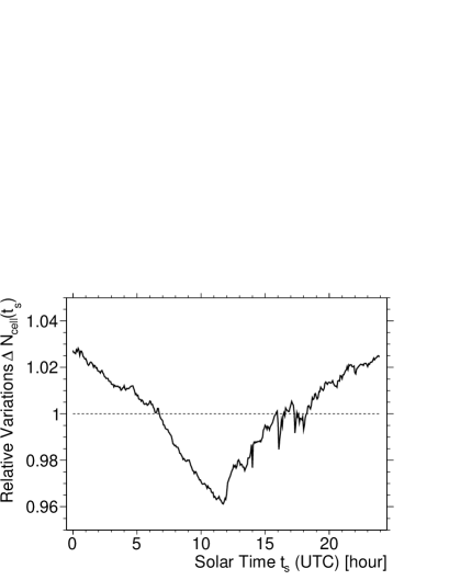
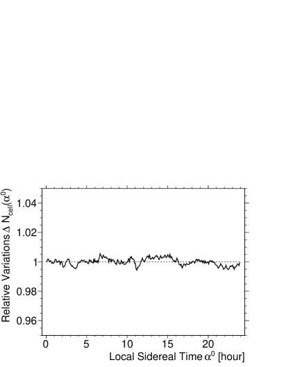
Figure 1: Relative variation of the integrated number of unitary cells as a function of the solar hour of the day in UTC (left panel), and as a function of the local sidereal time (right panel).

The instantaneous exposure $\omega(t,\theta,\phi,S_{38^{\circ}})$ of the SD array at the time $t$ as a function of the incident zenith and azimuth angles ($\theta,\phi$) and shower size $S_{38^{\circ}}$ is given by :

$$\omega(t,\theta,\phi,S_{38^{\circ}})=n_{\mathrm{cell}}(t)\times a_{\mathrm{cell}}\cos{\theta}\times\epsilon(S_{38^{\circ}},\theta,\phi),$$ (1)

where $a_{\mathrm{cell}}\cos{\theta}$ is the projected surface of a unitary cell under the incidence zenith angle $\theta$, $n_{\mathrm{cell}}(t)$ is the number of unitary cells at time $t$, and $\epsilon(S_{38^{\circ}},\theta,\phi)$ is the directional detection efficiency at size parameter $S_{38^{\circ}}$ under incidence angles ($\theta,\phi$). The conversion from $S_{38^{\circ}}$ to the energy $E$, which accounts for the changes of atmospheric conditions, will be presented in the next section.

The number of unitary cells $n_{\mathrm{cell}}(t)$ is recorded every second using the trigger system of the Observatory and reflects the array growth as well as the dead periods of each detector. It ranges from $\simeq 60$ (at the begining of the data taking in 2004) to $\simeq 1200$ (from the middle of 2008). From Eqn. 1, it is apparent that $n_{\mathrm{cell}}(t)$ is the only time-dependent quantity entering in the definition of the instantaneous exposure, modulating within any integrated solid angle the expected number of events as a function of time. For any periodicity $T$, the total number of unitary cells $N_{\mathrm{cell}}(t)$ as a function of time $t$ within a period and summed over all periods, and its associated relative variations $\Delta N_{\mathrm{cell}}(t)$ are obtained from :

$$N_{\mathrm{cell}}(t)=\sum_{j}n_{\mathrm{cell}}(t+jT),\hskip 28.45274pt\Delta N_{\mathrm{cell}}(t)=\frac{N_{\mathrm{cell}}(t)}{\left<N_{\mathrm{cell}}(t)\right>},$$ (2)

with $\left<N_{\mathrm{cell}}(t)\right>=1/T\,\int_{0}^{T}dt\,N_{\mathrm{cell}}(t)$.

A genuine dipolar anisotropy in the right ascension distribution of the events induces a modulation in the distribution of the time of arrival of events with a period equal to one sidereal day. A sidereal day indeed corresponds to the time it takes for the Earth to complete one rotation relative to the vernal equinox. It is approximately $T_{sid}=$ 23 hours, 56 minutes, 4.091 seconds. Throughout this article, we denote by $\alpha^{0}$ the local sidereal time and express it in hours or in radians, as appropriate. For practical reasons, $\alpha^{0}$ is chosen so that it is always equal to the right ascension of the zenith at the center of the array.

On the other hand, a dipolar modulation of experimental origin in the distribution of the time of arrival of events with a period equal to one solar day may induce a spurious dipolar anisotropy in the right ascension distribution of the events. Hence, it is essential to control $\Delta N_{\mathrm{cell}}(t)$ to account for the variation of the exposure in different directions. We show $\Delta N_{\mathrm{cell}}(t)$ in Fig. 1 in 360 bins of 4 minutes at these two time scales of particular interest : the solar one $T=T_{sol}$ = 24 hs (left panel), and the sidereal one $T=T_{sid}$ (right panel). A clear diurnal variation is apparent on the solar time scale showing an almost dipolar modulation with an amplitude of $\simeq 2.5$%. This is due to both the working times of the construction phase of the detector and to the outage of some batteries of the surface detector stations during nights. When averaged over 6 full years, this modulation is almost totally smoothed out on the sidereal time scale as seen in the right panel of Fig. 1. This distribution will be used in section 5.1.1 to weight the events when estimating the Rayleigh parameters.

From the instantaneous exposure, it is straightforward to compute the integrated exposure either in local coordinates $\omega(\theta,\phi,\alpha^{0})$ by replacing $n_{\mathrm{cell}}(t)$ by $\Delta N_{\mathrm{cell}}(\alpha^{0})$ in Eqn. 1, or in celestial coordinates $\omega(\alpha,\delta)$ by expressing the zenith angle $\theta$ in terms of the equatorial right ascension $\alpha$ and declination $\delta$ through :

$$\cos{\theta}=\sin{\ell_{\mathrm{site}}}\sin{\delta}+\cos{\ell_{\mathrm{site}}}\cos{\delta}\cos{(\alpha-\alpha^{0})},$$ (3)

(where $\ell_{\mathrm{site}}$ is the Earth latitude of the site) and then by integrating Eqn. 1 over time. Besides, let us also mention that to account for the spatial extension of the surface detector array making the latitude of the site $\ell_{\mathrm{site}}$ varying by $\simeq 0.4^{\circ}$, the celestial coordinates $(\alpha,\delta)$ of the events are calculated by transporting the showers to the "center" of the Observatory site.

4 Influence of the weather effects

Changes in the atmospheric pressure $P$ and air density $\rho$ have been shown to affect the development of extensive air showers detected by the surface detector array and these changes are reflected in the temporal variations of shower size at a fixed energy [20]. To eliminate these variations, the procedure used to convert the observed signal into energy needs to account for these atmospheric effects. This is performed by relating the signal at 1 km from the core, $S(1000)$, measured at the actual density $\rho$ and pressure $P$, to the one $\tilde{S}(1000)$ that would have been measured at reference values $\rho_{0}$ and $P_{0}$, chosen as the average values at Malargüe, i.e. $\rho_{0}=1.06$ kg m^-3 and $P_{0}=862$ hPa [20] :

$$\tilde{S}(1000)=\left[1-\alpha_{P}(\theta)(P-P_{0})-\alpha_{\rho}(\theta)(\rho_{d}-\rho_{0})-\beta_{\rho}(\theta)(\rho-\rho_{d})\right]S(1000),$$ (4)

where $\rho_{d}$ is the average daily density at the time the event was recorded. The measured coefficients $\alpha_{\rho}=(-0.80\pm 0.02)\,$kg^-1m³, $\beta_{\rho}=(-0.21\pm 0.02)\,$kg^-1m³ and $\alpha_{P}=(-1.1\pm 0.1)\,10^{-3}\,$hPa^-1 reflect respectively the impact of the variation of air density (and thus temperature) at long and short time scales, and of the variation of pressure on the shower sizes [20]. It is worth pointing out that air density coefficients are here predominant relative to the pressure one. The zenithal dependences of these parameters, that we use in the following, were also studied in reference [20]. It is this reference signal $\tilde{S}(1000)$ which has to be converted, using the constant intensity cut method, to the signal size $\tilde{S}_{38^{\circ}}$ and finally to energy. For convenience, we denote hereafter the uncorrected (corrected) shower size $S_{38^{\circ}}$ ($\tilde{S}_{38^{\circ}}$) simply by $S$ ($\tilde{S}$).

Carrying out such energy corrections is important for the study of large scale anisotro- pies. Above 3 EeV, the rate of events $R$ per unit time above a given uncorrected size threshold $S_{th}$, and in a given zenith angle bin, is modulated by changes of atmospheric conditions :

$$R(>S_{th})\propto\int_{S_{th}}^{\infty}dS\,\frac{dJ}{d\tilde{S}}\,\frac{d\tilde{S}}{dS}\propto\bigg{[}1+(\gamma_{S}-1)\,\alpha_{\xi}\,\Delta\xi\bigg{]}\,\int_{S_{th}}^{\infty}dS\,S^{-\gamma_{S}},$$ (5)

where hereafter $\xi$ generically denotes $P$, $\rho$ or $\rho_{d}$, and where we have adopted for the differential flux $dJ/dS$ a power law with spectral index $\gamma_{S}$. Hence, under changes of atmospheric parameters $\Delta\xi$, the following relative change in the rate of events is expected :

$$\frac{1}{R}\frac{dR(>S_{th})}{d\xi} \simeq (\gamma_{S}-1)\,\alpha_{\xi}.$$ (6)

Over a whole year, this spurious modulation is partially compensated in sidereal time, though not in solar time. In addition, a seasonal variation of the modulation of the daily counting rate induces sidebands at both the sidereal and anti-sidereal frequencies. This may lead to misleading measures of anisotropy if the amplitude of the sidebands significantly stands out above the background noise [21]. Correcting energies for weather effects, the net correction in the first harmonic amplitude in sidereal time turns out to be only of $\simeq 0.2\%$ for energy thresholds greater than 3 EeV, thanks to large cancellations taking place when considering the large time period used in this study.

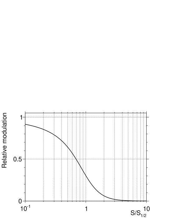
Figure 2: Relative modulation of the rates above a given corrected signal size due to the variations of the detection efficiency under changes of atmospheric conditions, relatively to the factor modulating the rate of events above the corresponding uncorrected signal size in units of $S_{1/2}$.

In addition to the energy determination, weather effects can also affect the detection efficiencies for showers with energies below 3 EeV, for the detection of which the surface array is not fully efficient. Changes of the shower signal size due to changes of weather conditions $\Delta\xi$ imply that showers are detected with the efficiency associated to the observed signal size $S$, which is related at first order to the one associated to the corrected signal size through :

$$\epsilon(S)\simeq\epsilon(\tilde{S})+(S-\tilde{S})\frac{d\epsilon(S)}{dS}\bigg{|}_{S=\tilde{S}}\simeq\epsilon(\tilde{S})+\alpha_{\xi}\Delta\xi\,\tilde{S}\,\frac{d\epsilon(S)}{dS}\bigg{|}_{S=\tilde{S}},$$ (7)

where we have made use of Eqn. 4. The second term modulates the observed rate of events, even after the correction of the signal sizes. Indeed, the rate of events $R$ above a given corrected signal size threshold $\tilde{S}_{th}$ is now the integration of the cosmic ray spectrum weighted by the corresponding detection efficiency expressed in terms of the observed signal size $S$ :

$$R(>\tilde{S}_{th})\propto\int_{\tilde{S}_{th}}^{\infty}d\tilde{S}\,\bigg{[}\epsilon(\tilde{S})+\alpha_{\xi}\Delta\xi\,\tilde{S}\,\frac{d\epsilon(S)}{dS}\bigg{|}_{S=\tilde{S}}\bigg{]}\,\frac{dJ}{d\tilde{S}}.$$ (8)

Hence, the relative change in the rate of events under changes in the atmosphere becomes :

$$\frac{1}{R}\frac{dR(>\tilde{S}_{th})}{d\xi}\simeq\frac{\alpha_{\xi}}{R}\int_{\tilde{S}_{th}}^{\infty}d\tilde{S}\,\tilde{S}\,\frac{dJ}{d\tilde{S}}\,\frac{d\epsilon(S)}{dS}\bigg{|}_{S=\tilde{S}},$$ (9)

which, after an integration by parts and at first order in $\alpha_{\xi}$, leads to :

$$\frac{1}{R}\frac{dR(>\tilde{S}_{th})}{d\xi} \simeq (\gamma_{S}-1)\,\alpha_{\xi}\,\bigg{[}1-\frac{\epsilon(\tilde{S}_{th})\int_{\tilde{S}_{th}}^{\infty}d\tilde{S}\,\tilde{S}^{-\gamma_{S}}}{\int_{\tilde{S}_{th}}^{\infty}d\tilde{S}\,\epsilon(\tilde{S})\,\tilde{S}^{-\gamma_{S}}}\bigg{]}.$$ (10)

The expression in brackets gives the additional modulations (in units of the weather effect modulation $(\gamma_{s}-1)\alpha_{\xi}$ when the detection efficiency is saturated) due to the variation of the detection efficiency. Note that this expression is less than 1 for any rising function $\epsilon$ satisfying $0\leq\epsilon(S)\leq 1$, and reduces to 0, as expected, when $\epsilon(\tilde{S}_{th})=1$. As a typical example, we show in Fig. 2 the expected modulation amplitude as a function of $S$ by adopting a reasonable detection efficiency function of the form $\epsilon(S)=S^{3}/\big{[}S^{3}+S_{1/2}^{3}\big{]}$ where the value of $S_{1/2}$ is such that $\epsilon(S_{1/2})=0.5$. This relative amplitude is about 0.3 for $S=S_{1/2}$, showing that for this signal size threshold the remaining modulation of the rate of events after the signal size corrections is about $0.3\times(\gamma_{s}-1)\alpha_{\xi}$. The value of $S_{1/2}$ being such that it corresponds to $\simeq 0.7$ EeV in terms of energy, it turns out that within the current statistics the Rayleigh analysis of arrival directions can be performed down to threshold energies of 1 EeV by only correcting the energy assignments.

5 Analysis methods and results

5.1 Overview of the analyses

The distribution in right ascension of the flux of CRs arriving at a detector can be characterised by the amplitudes and phases of its Fourier expansion, $I(\alpha)=I_{0}(1+r\cos(\alpha-\varphi)+r^{\prime}\cos(2(\alpha-\varphi^{\prime}))+\dots)$. Our aim is to determine the first harmonic amplitude $r$ and its phase $\varphi$. To account for the non-uniform exposure of the SD array, we perform two different analyses.

5.1.1 Rayleigh analysis weighted by exposure

Above 1 EeV, we search for the first harmonic modulation in right ascension by applying the classical Rayleigh formalism [13] slightly modified to account for the non-uniform exposure to different parts of the sky. This is achieved by weighting each event with a factor inversely proportional to the integrated number of unitary cells at the local sidereal time of the event (given by the right panel histogram of Fig. 1) [22, 23]:

$$a=\frac{2}{\mathcal{N}}\sum_{i=1}^{N}w_{i}\cos{\alpha_{i}},\hskip 28.45274ptb=\frac{2}{\mathcal{N}}\sum_{i=1}^{N}w_{i}\sin{\alpha_{i}},$$ (11)

where the sum runs over the number of events $N$ in the considered energy range, the weights are given by $w_{i}\equiv[\Delta N_{\mathrm{cell}}(\alpha^{0}_{i})]^{-1}$ and the normalisation factor is $\mathcal{N}=\sum_{i=1}^{N}w_{i}$. The estimated amplitude $r$ and phase $\varphi$ are then given by :

$$r=\sqrt{a^{2}+b^{2}},\hskip 28.45274pt\varphi=\arctan\frac{b}{a}.$$ (12)

As the deviations from an uniform right ascension exposure are small, the probability $P(>r)$ that an amplitude equal or larger than $r$ arises from an isotropic distribution can be approximated by the cumulative distribution function of the Rayleigh distribution $P(>r)=\exp{(-k_{0})}$, where $k_{0}=\mathcal{N}r^{2}/4$.

5.1.2 East-West method

Below 1 EeV, due to the variations of the event counting rate arising from Eqn. 10, we adopt the differential East-West method [14]. Since the instantaneous exposure of the detector for Eastward and Westward events is the same, with both sectors being equally affected by the instabilities of the detector and the weather conditions, the difference between the event counting rate measured from the East sector, $I_{E}(\alpha^{0})$, and the West sector, $I_{W}(\alpha^{0})$, allows us to remove at first order the direction independent effects of experimental origin without applying any correction, though at the cost of a reduced sensitivity. Meanwhile, this counting difference is directly related to the right ascension modulation $r$ by (see Appendix) :

$$I_{E}(\alpha^{0})-I_{W}(\alpha^{0})=-\frac{N}{2\pi}\frac{2\left<\sin{\theta}\right>}{\pi\langle\cos\delta\rangle}r\sin(\alpha^{0}-\varphi).$$ (13)

The amplitude $r$ and phase $\varphi$ can thus be calculated from the arrival times of each set of $N$ events using the standard first harmonic analysis [13] slightly modified to account for the subtraction of the Western sector to the Eastern one. The Fourier coefficients $a_{EW}$ and $b_{EW}$ are thus defined by :

$$a_{EW}=\frac{2}{N}\sum_{i=1}^{N}\cos{(\alpha^{0}_{i}+\zeta_{i})},\hskip 28.45274ptb_{EW}=\frac{2}{N}\sum_{i=1}^{N}\sin{(\alpha^{0}_{i}+\zeta_{i})},$$ (14)

where $\zeta_{i}$ equals 0 if the event is coming from the East or $\pi$ if coming from the West (so as to effectively subtract the events from the West direction). This allows us to recover the amplitude $r$ and the phase $\varphi_{EW}$ from

$$r=\sqrt{a_{EW}^{2}+b_{EW}^{2}},\hskip 28.45274pt\varphi_{EW}=\arctan{\left(\frac{b_{EW}}{a_{EW}}\right)}.$$ (15)

Note however that $\varphi_{EW}$, being the phase corresponding to the maximum in the differential of the East and West fluxes, is related to $\varphi$ in Eqn. 12 through $\varphi=\varphi_{EW}+\pi/2$. As in the previous analysis, the probability $P(>r)$ that an amplitude equal or larger than $r$ arises from an isotropic distribution is obtained by the cumulative distribution function of the Rayleigh distribution $P(>r)=\exp{(-k_{0}^{EW})}$, where $k_{0}^{EW}=(2\left<\sin{\theta}\right>/\pi\langle\cos\delta\rangle)^{2}\times Nr^{2}/4$. For the values of $\left<\sin{\theta}\right>$ and $\langle\cos\delta\rangle$ of the events used in this analysis, the first factor in the expression for $k_{0}^{EW}$ is 0.22. Then, comparing it with the expression for $k_{0}$ in the standard Rayleigh analysis, it is seen that approximately four times more events are needed in the East-West method to attain the same sensitivity to a given amplitude $r$.

5.2 Analysis of solar, anti-sidereal, and random frequencies

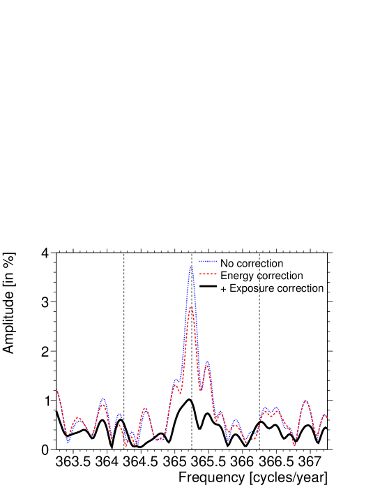
Figure 3: Amplitude of the Fourier modes as a function of the frequency above 1 EeV. Thin dotted curve : before correction of energies and exposure. Dashed curve : after correction of energies but before correction of exposure. Thick curve : After correction of energies and exposure. Dashed vertical lines from left to right : anti-sidereal, solar and sidereal frequencies.

The amplitude $r$ corresponds to the value of the Fourier transform of the arrival time distribution of the events at the sidereal frequency. This can be generalised to other frequencies by performing the Fourier transform of the modified time distribution [24] :

$$\tilde{\alpha}^{0}_{i}=\frac{2\pi}{T_{sid}}t_{i}+\alpha_{i}-\alpha^{0}_{i}.$$ (16)

Such a generalisation is helpful for examining an eventual residual spurious modulation after applying the Rayleigh analysis after the corrections discussed in Sections 3 and 4. The amplitude of the Fourier modes when considering all events above 1 EeV are shown in Fig. 3 as a function of the frequency in a window centered on the solar one (indicated by the dashed line at 365.25 cycles/year). The thin dotted curve is obtained without accounting for the variations of the exposure and without accounting for the weather effects. The large period of time analysed here, over 6 years, allows us to resolve the frequencies at the level of $\simeq 1/6$ cycles/year. This induces a large decoupling of the frequencies separated by more than this resolution [24]. In particular, as the resolution is less than the difference between the solar and the (anti-)sidereal frequencies (which is of 1 cycle/year), this explains why the large spurious modulations standing out from the background noise around the solar frequency are largely averaged out at both the sidereal and anti-sidereal frequencies even without applying any correction. The impact of the correction of the energies discussed in Section 4 is evidenced by the dashed curve, which shows a reduction of $\simeq 30$% of the spurious modulations within the resolved solar peak. In addition, when accounting also for the exposure variation at each frequency, the solar peak is reduced at a level close to the statistical noise, as evidenced by the thick curve. Results at the solar and the anti-sidereal frequencies are collected in Tab. 1.

	$r_{\mathrm{solar}}$[%]	$P(>r_{\mathrm{solar}})$[%]	$r_{\mathrm{anti-sid}}$[%]	$P(>r_{\mathrm{anti-sid}})$[%]
no correction	3.7	$\simeq 2\,10^{-37}$	0.36	43
energy corrections	2.9	$\simeq 4\,10^{-23}$	0.15	85
+exposure correction	0.96	0.2	0.49	19

Table 1: Amplitude and corresponding probability to get a larger amplitude from an isotropic distribution at both the solar and the anti-sidereal frequencies for events with energies $>1\,$EeV.

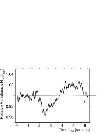
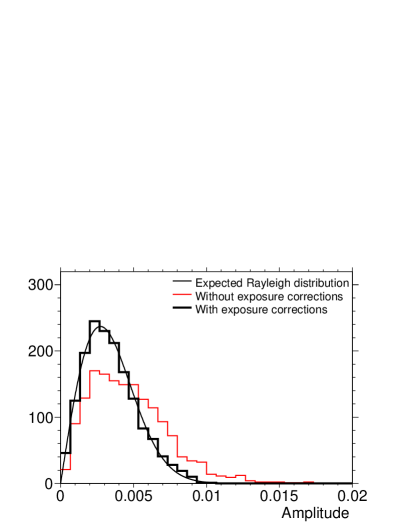
Figure 4: Left : Relative variation of the integrated number of unitary cells as a function of the time $t_{100}$, where the time scale is such that corresponding frequency is 100 cycles/year. Right : Rayleigh analysis above 1 EeV for 1600 random frequencies ranging from 100 to 500 cycles/year. Thin histogram : analysis without accounting for the exposure variations. Thick histogram : analysis accounting for the exposure variations. Smooth curve : expected Rayleigh distribution.

To provide further evidence of the relevance of the corrections introduced to account for the non-uniform exposure, it is worth analysing on a statistical basis the behaviour of the reconstructed amplitudes at different frequencies (besides the anti-sidereal/solar/sidereal ones). In particular, as the number of unitary cells $n_{\mathrm{cell}}$ has increased from $\simeq$ 60 to $\simeq$ 1200 over the 6 years of data taking, an automatic increase of the variations of $\Delta N_{\mathrm{cell}}(t)$ is expected at large time periods. This expectation is illustrated in the left panel of Fig. 4, which is similar to Fig. 1 but at a time periodicity $T\simeq 87.5\,$h, corresponding to a low frequency of 100 cycles/year. The size of the modulation is of the order of the one observed in Fig. 1 at the solar frequency. In the right panel of Fig. 4, the results of the Rayleigh analysis applied above 1 EeV to 1600 random frequencies ranging from 100 to 500 cycles/year are shown by histograming the reconstructed amplitudes. The thin one is obtained without accounting for the variations of the exposure : it clearly deviates from the expected Rayleigh distribution displayed in the same graph. Once the exposure variations are accounted for through the weighting procedure, the thick histogram is obtained, now in agreement with the expected distribution. Note that in both cases the energies are corrected for weather effects, but the impact of these effects is marginal when considering such random frequencies. This provides additional support that the variations of the counting rate induced by the variations of the exposure are under control through the monitoring of $\Delta N_{\mathrm{cell}}(t)$.

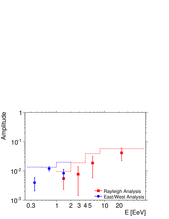
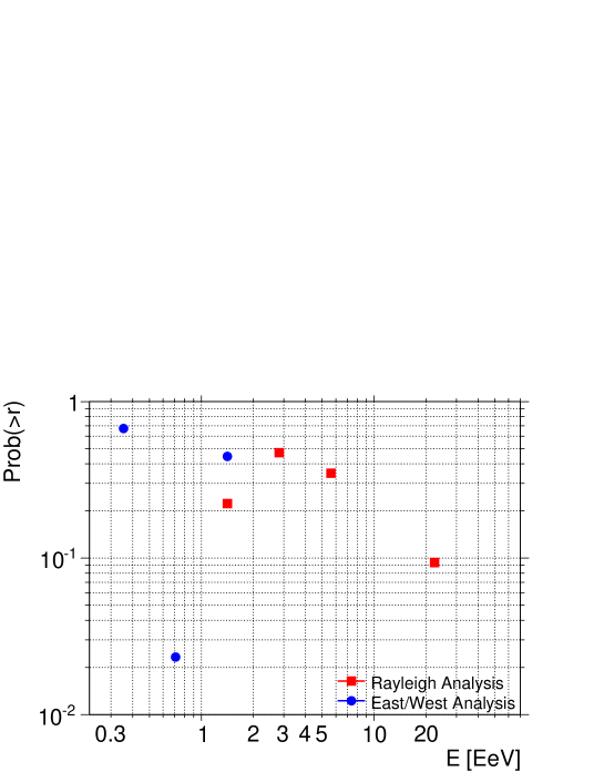
Figure 5: Top : Amplitude of the first harmonic as a function of energy. The dashed line indicates the 99% $C.L.$ upper bound on the amplitudes that could result from fluctuations of an isotropic distribution. Bottom : Corresponding probabilities to get at least the same amplitude from an underlying isotropic distribution.

5.3 Results at the sidereal frequency in independent energy bins

To perform first harmonic analyses as a function of energy, the choice of the size of the energy bins, although arbitrary, is important to avoid the dilution of a genuine signal with the background noise. In addition, the inclusion of intervals whose width is below the energy resolution or with too few data is most likely to weaken the sensitivity of the search for an energy-dependent anisotropy [25]. To fulfill both requirements, the size of the energy intervals is chosen to be $\Delta\log_{10}(E)=0.3$ below 8 EeV, so that it is larger than the energy resolution even at low energies. At higher energies, to guarantee the determination of the amplitude measurement within an uncertainty $\sigma\simeq 2\%$, all events ($\simeq 5,000$) with energies above 8 EeV are gathered in a single energy interval.

The amplitude $r$ at the sidereal frequency as a function of the energy is shown in Fig. 5, together with the corresponding probability $P(>r)$ to get a larger amplitude in each energy interval for a statistical fluctuation of isotropy. The dashed line indicates the 99% $C.L.$ upper bound on the amplitudes that could result from fluctuations of an isotropic distribution. It is apparent that there is no evidence of any significant signal over the whole energy range. A global statement refering to the probability with which the 6 observed amplitudes could have arisen from an underlying isotropic distribution can be made by comparing the measured value $K=\sum_{i=1}^{6}k_{0_{i}}$ (where the sum is over all 6 independent energy intervals) with that expected from a random distribution for which $\left<K\right>=6$ [26]. The statistics of $2K$ under the hypothesis of an isotropic sky is a $\chi^{2}$ with $2\times 6=12$ degrees of freedom. For our data, $2K=19.0$ and the associated probability for an equal or larger value arising from an isotropic sky is $\simeq 9$%.

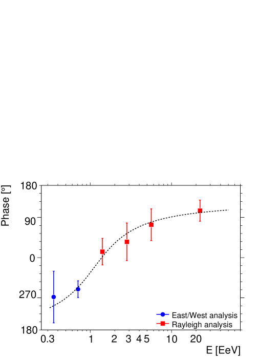
Figure 6: Phase of the first harmonic as a function of energy. The dashed line, resulting from an empirical fit, is used in the likelihood ratio test (see text).

The phase $\varphi$ of the first harmonic is shown in Fig. 6 as a function of the energy. While the measurements of the amplitudes do not provide any evidence for anisotropy, we note that the measurements in adjacent energy intervals suggest a smooth transition between a common phase of $\simeq 270^{\circ}$ in the first two bins below $\simeq 1$ EeV compatible with the right ascension of the Galactic Center $\alpha_{GC}\simeq 268.4^{\circ}$, and another phase ($\alpha\simeq 100^{\circ}$) above $\simeq 5$ EeV. This is intriguing, as the phases are expected to be randomly distributed in case of independent samples whose parent distribution is isotropic. Knowing the p.d.f. of phase measurements drawn from an isotropic distribution, $p_{0}(\varphi)=(2\pi)^{-1}$, and drawn from a population of directions having a non-zero amplitude $r_{0}$ with a phase $\varphi_{0}$, $p_{1}(\varphi;r_{0},\varphi_{0})$ [13], the likelihood functions of any of the hypotheses may be built as :

$$L_{0}=\prod_{i=1}^{N_{bins}}p_{0}(\varphi_{i}),\hskip 28.45274ptL_{1}=\prod_{i=1}^{N_{bins}}p_{1}(\varphi_{i};r_{0},\varphi_{0}).$$ (17)

Without any knowledge of the expected amplitudes $r_{0}(E)$ in each bin, the values considered in $L_{1}$ are the measurements performed in each energy interval. For the expected phases $\varphi_{0}(E)$ as a function of energy, we use an arctangent function adjusted on the data as illustrated by the dashed line in Fig. 6. Since the smooth evolution of the phase distribution is potentially interesting but observed a posteriori, we aim at testing the fraction of random samples whose behaviour in adjacent energy bins would show such a potential interest but with no reference to the specific values observed in the data. To do so, we use the method of the likelihood ratio test, computing the $-2\ln(\lambda)$ statistic where $\lambda=L_{0}/L_{1}$. Using only $N_{bins}=6$, the asymptotic behaviour of the $-2\ln(\lambda)$ statistic is not reached. Hence, the p.d.f. of $-2\ln(\lambda)$ under the hypothesis of isotropy is built by repeating exactly the same procedure on a large number of isotropic samples : in each sample, the arctangent parameters are left to be optimised, and the corresponding value of $-2\ln(\lambda)$ is calculated. In that way, any alignments, smooth evolutions or abrupt transitions of phases in random samples are captured and contribute to high values of the $-2\ln(\lambda)$ distribution. The probability that the hypothesis of isotropy better reproduces our phase measurements compared to the alternative hypothesis is then calculated by integrating the normalised distribution of $-2\ln(\lambda)$ above the value measured in the data. It is found to be $\simeq 2\cdot 10^{-3}$.

It is important to stress that no confidence level can be built from this report as we did not perform an a priori search for a smooth transition in the phase measurements. To confirm the detection of a real transition using only the measurements of the phases with an independent data set, we need to collect $\simeq 1.8$ times the number of events analysed here to reach an efficiency of $\simeq 90\%$ to detect the transition at 99% $C.L.$ (in case the observed effect is genuine). It is also worth noting that with a real underlying anisotropy, a consistency of the phase measurements in ordered energy intervals is expected with lower statistics than the detection of amplitudes significantly standing out of the background noise [26, 27]. This behaviour was pointed out by Linsley, quoted in [26] : “if the number of events available in an experiment is such that the RMS value of $r$ is equal to the true amplitude, then in a sequence of experiments $r$ will be significant (say $P(>r)<1\%$) in one experiment out of ten whereas the phase will be within 50^∘ of the true phase in two experiments out of three.” We have checked this result using Monte Carlo simulations.

An apparent constancy of phase, even when the significances of the amplitudes are relatively small, has been noted previously in surveys of measurements made in the range $10^{14}<E<10^{17}\,$eV [28, 29]. In [28] Greisen and his colleagues comment that most experiments have been conducted at northern latitudes and therefore the reality of the sidereal waves is not yet established. The present measurement is made with events coming largely from the southern hemisphere.

5.4 Additional cross-checks against systematic effects above 1 EeV

It is important to verify that the phase effect is not a manifestation of systematic effects, the amplitudes of which are at the level of the background noise. We provide hereafter additional studies above 1 EeV, where a few tests can cross-check results presented in Fig. 6.

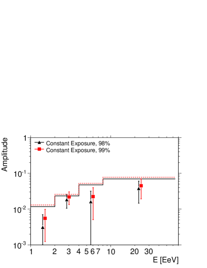
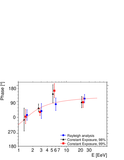
Figure 7: Rayleigh analysis above 1 EeV using a reduced data set built to get at a constant exposure in right-ascension, using on-times of 98% (triangles) and 99% (squares) (see text). Left : analysis of the amplitude. The full (dashed) line indicates the 99% $C.L.$ upper bound on the amplitudes that could result from fluctuations of an isotropic distribution when using on-times of 98% (99%). Right : analysis of the phase, the dashed line being the same as the one plotted in Fig. 6. Results of Fig. 6 are also shown with circles.

The first cross-check is provided by applying the Rayleigh analysis on a reduced data set built in such a way that its corresponding exposure in right ascension is uniform. This can be achieved by selecting for each sidereal day only events triggering an unitary cell whose on-time was almost 100% over the whole sidereal day. To keep a reasonably large data set, we present here the results obtained for on-times of 98% and 99%. This allows us to use respectively $\simeq 77$% and $\simeq 63$% of the cumulative data set without applying any correction to account for a non-constant exposure. The results are shown in Fig. 7 when considering on-time of 98% (triangles) and 99% (squares). Even if more noisy due to the reduction of the statistics with respect to the Rayleigh analysis applied on the cumulative data set, they are consistent with the weighted Rayleigh analysis and support that results presented in Fig. 6 are not dominated by any residual systematics induced by the non-uniform exposure.

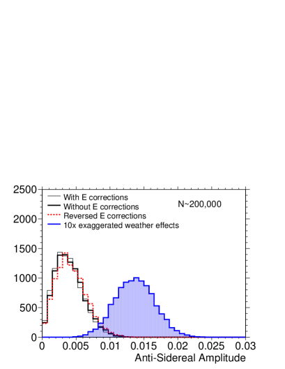
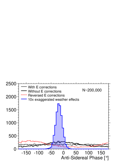
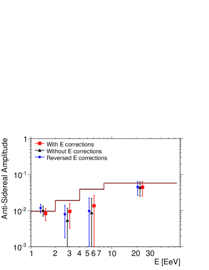
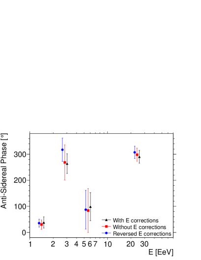
Figure 8: Top :Anti-sidereal analysis of mock samples built such that a spurious anti-sidereal amplitude stands out from the noise through the sideband mechanism between 1 and 2 EeV (see text). Thin histograms : standard Rayleigh analysis of the amplitudes (left panel) and phases (right panel) for isotropic samples. Thick histograms : same for samples biased by the energy variations induced by the atmospheric changes. Dashed histograms : same by reversing the energy corrections. Filled histograms : same by amplifying by 10 the energy variations. Bottom : Rayleigh analysis of the anti-sidereal amplitude (left) and phase (right) of the real data sample without applying the energy corrections (squares), by applying those corrections (triangles), and by reversing the energy corrections (circles).

From the Fourier analysis presented in section 5.2, we have stressed the decoupling between the solar frequency and both the sidereal and anti-sidereal ones thanks to the frequency resolution reached after 6 years of data taking. However, as the amplitude of an eventual sideband effect is proportional to the solar amplitude  [21], it remains important to estimate the impact of an eventual sideband effect persisting even after the energy corrections. To probe the magnitude of this sideband effect, we use 10,000 mock data sets generated from the real data set (with energies corrected for weather effects) by randomising the arrival times but meanwhile keeping both the zenith and the azimuth angles of each original event. This procedure guarantees the production of isotropic samples drawn from a uniform exposure with the same detection efficiency conditions than the real data. The results of the Rayleigh analysis applied to each mock sample between 1 and 2 EeV at the anti-sidereal frequency are shown by the thin histograms in top panels of Fig. 8, displaying Rayleigh distributions for the amplitude measurements and uniform distributions for the phase measurements. Then, after introducing in to each sample the temporal variations of the energies induced by the atmospheric changes according to Eqn. 4, it can be seen on the same graph (thick histograms) that the amplitude measurements are almost undistinguishable with respect to the reference ones, while the phase measurements start to show to a small extent a preferential direction. The same conclusions hold when reversing the energy corrections (dashed histograms), but resulting in a phase shift of $\simeq 180^{\circ}$. Finally, the filled histograms are obtained by amplifying by 10 the energy variations induced by the atmospheric changes. In this latter case, the large increase of the solar amplitude induces a clear signal at the anti-sidereal frequency through the sideband mechanism, as evidenced by the distributions of both the amplitudes and the phases. The sharp maximum of the phase distribution points towards the spurious direction, while the amplitude distribution follows a non-centered Rayleigh distribution with parameter $\simeq 1.4\times 10^{-2}$. The spurious mean amplitude stands out from the noise ($\sim\sqrt{\pi/200,000}\simeq 4\times 10^{-3}$) sufficiently to allow us to estimate empirically the original effect to be ten times smaller, at the level of $\simeq 1.4\times 10^{-3}$. This will impact the analyses only in a marginal way even if we had not performed the energy corrections, or if we had over-corrected the energies. The energy corrections necessarily reduce even more the size of the sideband amplitude, well below $\simeq 10^{-3}$. Hence, only small changes are expected in the anti-sidereal phase measurements on the real data when applying (or not) or reversing the energy corrections. This is found to be the case, as illustrated in the bottom panels of Fig. 8. In addition, this phase distribution (bottom right panel of Fig. 8) does not show any particular structure aligned with the spurious direction. This second cross-check support the hypothesis that the phase measurements presented in Fig. 6 are not dominated by any residual systematics induced by the sideband mechanism.

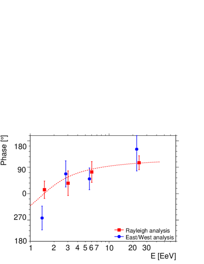
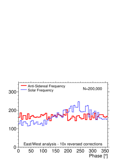
Figure 9: Left : East/West analysis at the sidereal frequency above 1 EeV. Right : East/West analyses at both the solar (dashed) and the anti-sidereal (thick) frequencies of mock samples built by amplifying by 10 the energy variations induced by weather effects.

In the left panel of Fig. 9 we show the results of the East/West analysis (circles). They provide further support of the previous analyses (squares). As previously explained, this method relies on the high symmetry between the Eastern and Western sectors. However, the array being slightly tilted ($\simeq 0.2^{\circ}$), this symmetry is slightly broken, resulting in a small shift between the Eastward and Westward counting rates. As this shift is independent of time, it does not impact itself in the estimate of the first harmonic. However, it is worth examining the effect of the combination of the tilted array together with the spurious modulations induced by weather effects, as this combination may mimic a real East/West first harmonic modulation at the solar frequency. The size of such an effect can be probed by analysing the mock data sets built by amplifying by 10 the energy variations induced by the atmospheric changes. The results obtained between 1 and 2 EeV at both the solar and the anti-sidereal frequencies are shown in the right panel of Fig. 9 : while the phase distribution starts to show a preferential direction at the solar frequency (dashed histogram), the same distribution is still uniform at the anti-sidereal one (thick histogram). Hence, it is safe to conclude that the results obtained at the sidereal frequency by means of the East/West method are not affected by any systematics.

5.5 Results at the sidereal frequency in cumulative energy bins

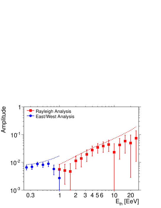
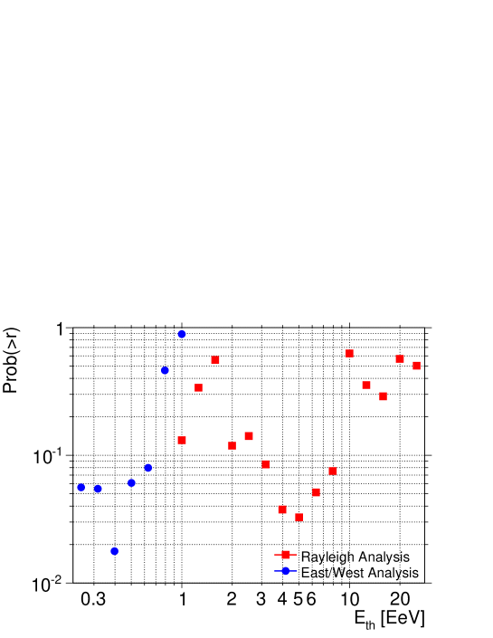
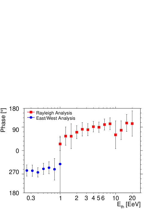
Figure 10: Same as Fig. 5 and Fig. 6, but as a function of energy thresholds.

Performing the same analysis in terms of energy thresholds may be convenient for optimizing the detection of an eventual genuine signal spread over a large energy range, avoiding the arbitrary choice of a bin size $\Delta\log_{10}(E)$. The bins are however strongly correlated, preventing a straightforward interpretation of the evolution of the points with energy. The results on the amplitudes are shown in Fig. 10. They do not provide any further evidence in favor of a significant amplitude.

6 Upper limits and discussion

$\Delta E$	$N$	$r_{\mathrm{sidereal}}$[%]	$P(>r_{\mathrm{sidereal}})[\%]$	$\varphi$ [∘]	$\Delta\varphi$ [∘]	$d_{\perp}^{UL}$ [%]
0.25 - 0.5	553639	0.4	67	262	64	1.3
0.5 - 1	488587	1.2	2	281	20	1.7
1 - 2	199926	0.5	22	15	33	1.4
2 - 4	50605	0.8	47	39	46	2.3
4 - 8	12097	1.8	35	82	39	5.5
$>$8	5486	4.1	9	117	27	9.9

Table 2: Results of first harmonic analyses in different energy intervals, using the East/West analysis below 1 EeV and the Rayleigh analysis above 1 EeV.

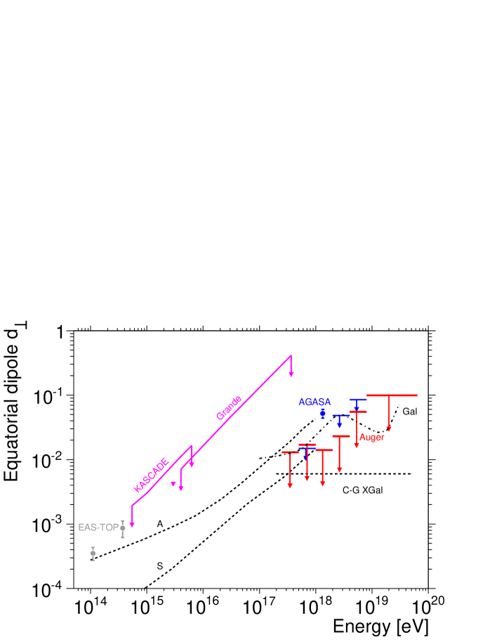
Figure 11: Upper limits on the anisotropy amplitude of first harmonic as a function of energy from this analysis. Results from EAS-TOP, AGASA, KASCADE and KASCADE-Grande experiments are displayed too. An analysis of the KASCADE-Grande data with the East/West method delivers an additional limit for $3\,10^{15}\,$eV. Also shown are the predictions up to 1 EeV from two different galactic magnetic field models with different symmetries ($A$ and $S$), the predictions for a purely galactic origin of UHECRs up to a few tens of $10^{19}\,$eV ($Gal$), and the expectations from the Compton-Getting effect for an extragalactic component isotropic in the CMB rest frame ($C$-$G\,Xgal$).

From the analyses reported in the previous Section, upper limits on amplitudes at 99% $C.L.$ can be derived according to the distribution drawn from a population characterised by an anisotropy of unknown amplitude and phase as derived by Linsley [13] :

$$\sqrt{\frac{2}{\pi}}\frac{1}{I_{0}(r^{2}/4\sigma^{2})}\int_{0}^{r_{UL}}\frac{\mathrm{d}s}{\sigma}\,I_{0}\bigg{(}\frac{rs}{\sigma^{2}}\bigg{)}\,\exp{\bigg{(}-\frac{s^{2}+r^{2}/2}{2\sigma^{2}}\bigg{)}}=C.L.,$$ (18)

where $I_{0}$ is the modified Bessel function of the first kind with order 0, and $\sigma=\sqrt{2/\mathcal{N}}$ in case of the Rayleigh analysis, and $\sigma_{EW}=(\pi\left<\cos{\delta}\right>/2\left<\sin{\theta}\right>)\times\sqrt{2/N}$ in case of the East/West analysis.

As discussed in the Appendix, the Rayleigh amplitude measured by an observatory depends on its latitude and on the range of zenith angles considered. The measured amplitude can be related to a real equatorial dipole component $d_{\perp}$ by $d_{\perp}\simeq r/\langle\cos\delta\rangle$. This is the physical quantity of interest to compare results from different experiments and from model predictions. The upper limits on $d_{\perp}$ are given in Tab. 2 and shown in Fig.11, together with previous results from EAS-TOP [11], KASCADE [31], KASCADE-Grande [32] and AGASA [33], and with some predictions for the anisotropies arising from models of both galactic and extragalactic UHECR origin. The results obtained in this study are not consistent with the $\simeq 4$% anisotropy reported by AGASA in the energy range $1<E/\mathrm{EeV}<2$.

If the galactic/extragalactic transition occurs at the ankle energy [1], UHECRs at 1 EeV are predominantly of galactic origin and their escape from the galaxy by diffusion and drift motions are expected to induce a modulation in this energy range. These predictions depend on the assumed galactic magnetic field model as well as on the source distribution and the composition of the UHECRs. Two alternative models are displayed in Fig. 11, corresponding to different geometries of the halo magnetic fields [9]. The bounds reported here already exclude the particular model with an antisymmetric halo magnetic field ($A$) and are starting to become sensitive to the predictions of the model with a symmetric field ($S$). We note that those models assume a predominantly heavy composition galactic component at EeV energies, while scenarios in which galactic protons dominate at those energies would typically predict anisotropies larger than the bounds obtained in Fig. 11. Maintaining the amplitudes of such anisotropies within our bounds necessarily translates into constraints upon the description of the halo magnetic fields and/or the spatial source distribution. This is particularly interesting in the view of our composition measurements at those energies compatible with a light composition [34]. Aternatively to a leaky galaxy model, there is still the possibility that a large scale magnetic field retains all particles in the galaxy [35, 36]. If the structure of the magnetic fields in the halo is such that the turbulent component predominates over the regular one, purely diffusion motions may confine light elements of galactic origin up to $\simeq 1\,$EeV and may induce an ankle feature due to the longer confinement of heavier elements at higher energies [37]. Typical signatures of such a scenario in terms of large scale anisotropies are also shown in Fig. 11 (dotted line) : the corresponding amplitudes are challenged by our current sensitivity.

On the other hand, if the transition is taking place at lower energies around the second knee at $\simeq 5\times 10^{17}\,$eV [7], UHECRs above 1 EeV are dominantly of extragalactic origin and their large scale distribution could be influenced by the relative motion of the observer with respect to the frame of the sources. If the frame in which the UHECR distribution is isotropic coincides with the CMB rest frame, a small anisotropy is expected due to the Compton-Getting effect. Neglecting the effects of the galactic magnetic field, this anisotropy would be a dipolar pattern pointing in the direction $\alpha\simeq 168^{\circ}$ with an amplitude of about 0.6% [38]. On the contrary, when accounting for the galactic magnetic field, this dipolar anisotropy is expected to also affect higher order multipoles [39]. These amplitudes are close to the upper limits set in this analysis, and the statistics required to detect an amplitude of 0.6% at 99% $C.L.$ is $\simeq 3$ times the present one.

Continued scrutiny of the large scale distribution of arrival directions of UHECRs as a function of energy with the increased statistics provided by the Pierre Auger Observatory, above a few times $10^{17}\,$eV, will help to discriminate between a predominantly galactic or extragalactic origin of UHECRs as a function of the energy, and so benefit the search for the galactic/extragalactic transition. Future work will profit from the lower energy threshold that is now available at the Pierre Auger Observatory [40].

This article is dedicated to Gianni Navarra, who has been deeply involved in this study for many years and who has inspired several of the analyses described in this paper. His legacy lives on.

Appendix

The first harmonic amplitude of the distribution in right ascension of the detected cosmic rays can be directly related to the amplitude $d$ of a dipolar distribution of the cosmic ray flux of the form $J(\alpha,\delta)=J_{0}(1+d\ \hat{d}\cdot\hat{u})$, where $\hat{u}$ and $\hat{d}$ denote respectively the unit vector in the direction of an arrival direction and in the direction of the dipole. Eqn. 11 and Eqn. 12 can be used to express $a$, $b$ and $\mathcal{N}$ as :

$$a = \frac{2}{\mathcal{N}}\int_{\delta_{min}}^{\delta_{max}}d\delta\int_{0}^{2\pi}d\alpha\cos\delta\ J(\alpha,\delta)\ \omega(\delta)\cos\alpha,$$ (19)

$$b = \frac{2}{\mathcal{N}}\int_{\delta_{min}}^{\delta_{max}}d\delta\int_{0}^{2\pi}d\alpha\cos\delta\ J(\alpha,\delta)\ \omega(\delta)\sin\alpha,$$

$$\mathcal{N} = \int_{\delta_{min}}^{\delta_{max}}d\delta\int_{0}^{2\pi}d\alpha\cos\delta\ J(\alpha,\delta)\ \omega(\delta),$$

where we have here neglected in the exposure $\omega$ the small dependence on right ascension. Writing the angular dependence in $J(\alpha,\delta)$ as $\hat{d}\cdot\hat{u}=\cos\delta\cos\delta_{d}\cos(\alpha-\alpha_{d})+\sin\delta\sin\delta_{d}$, with $\delta_{d}$ the dipole declination and $\alpha_{d}$ its right ascension, and performing the integration in $\alpha$ in the previous equations, it can be seen that

$$r=\left|\frac{Ad_{\perp}}{1+Bd_{z}}\right|$$ (20)

where

$$A=\frac{\int d\delta\,\omega(\delta)\cos^{2}\delta}{\int d\delta\,\omega(\delta)\cos\delta},\hskip 28.45274ptB=\frac{\int d\delta\,\omega(\delta)\cos\delta\sin\delta}{\int d\delta\,\omega(\delta)\cos\delta}$$

and $d_{z}=d\sin{\delta_{d}}$ denotes the component of the dipole along the Earth rotation axis while $d_{\perp}=d\cos{\delta_{d}}$ is the component in the equatorial plane [30]. The coefficients $A$ and $B$ can be estimated from the data as the mean values of the cosine and the sine of the event declinations. In our case, $A=\left<\cos{\delta}\right>\simeq 0.78$ and $B=\left<\sin{\delta}\right>\simeq-0.45$. For a dipole amplitude $d$, the measured amplitude of the first harmonic in right ascension $r$ thus depends on the region of the sky observed, which is essentially a function of the latitude of the observatory $\ell_{site}$, and the range of zenith angles considered. In the case of a small $Bd_{z}$ factor, the dipole component in the equatorial plane $d_{\perp}$ is obtained as $d_{\perp}\simeq r/\left<\cos{\delta}\right>$. The phase $\varphi$ corresponds to the right ascension of the dipole direction $\alpha_{d}$.

Turning now to the East-West method, the measured flux from the East sector for a local sidereal time $\alpha^{0}$ can be similarly expressed as

$$I_{E}(\alpha^{0})=\int_{-\pi/2}^{\pi/2}d\phi\int_{0}^{\theta_{max}}d\theta\sin\theta\ \epsilon(\theta)\ J(\theta,\phi,\alpha^{0}),$$ (21)

and analogously for the measured flux coming from the west sector changing the azimuthal integration to the interval $[\pi/2,3\pi/2]$. Expressing $\hat{d}\cdot\hat{u}$ in local coordinates ($\theta$, $\phi$ and $\alpha^{0}$), and performing the integration over $\phi$ we obtain for the leading order

$$\frac{I_{E}-I_{W}}{\langle I_{E}+I_{W}\rangle}(\alpha^{0})=-\frac{2d_{\perp}C}{\pi(1+d_{z}D\sin\ell_{site})}\sin(\alpha^{0}-\alpha_{d}),$$ (22)

where

$$C=\frac{\int d\theta\,\epsilon(\theta)\sin^{2}\theta}{\int d\theta\,\epsilon(\theta)\sin\theta},\hskip 28.45274ptD=\frac{\int d\theta\,\epsilon(\theta)\sin\theta\cos\theta}{\int d\theta\,\epsilon(\theta)\sin\theta}.$$

In this calculation any dependence of the exposure on the local sidereal time $\alpha^{0}$ gives at first order the same contribution to the East and West sectors flux, and thus gives a negligible contribution to the flux difference. The next leading order, proportional to the equatorial dipole component times the sidereal modulation of the exposure, is negligible. The coefficients $C$ and $D$ can be estimated from the observed zenith angles of the events. In our case, $C=\left<\sin\theta\right>\simeq 0.58$ and $D=\left<\cos\theta\right>\simeq 0.78$. The total detected flux averaged over the local sidereal time can be estimated as $\langle I_{E}+I_{W}\rangle=N/2\pi$. In case $Dd_{z}\ll 1$, we get finally :

$$(I_{E}-I_{W})(\alpha^{0})=-\frac{N}{2\pi}\frac{2d_{\perp}\langle\sin\theta\rangle}{\pi}\sin(\alpha^{0}-\alpha_{d}).$$ (23)

References

References

- [1] J. Linsley, Proceedings of the 8th Int. Conf. on Cosmic Rays, Jaipur 4 (1963) 77
- [2] M.A. Lawrence, R.J.O. Reid, and A.A. Watson, J. Phys. G17 (1991) 733
- [3] M. Nagano et al., J. Phys. G18 (1992) 423
- [4] D.J. Bird et al., (Flys Eye Collab.), Phys. Rev. Lett. 71 (1993) 3401
- [5] The Auger Collaboration, Phys. Lett. B 685 (2010) 239
- [6] A.M. Hillas, Phys. Lett. 24, (1967) 677
- [7] V. Berezinsky et al., Astron. and Astrophys. 043005 (2006) 74
- [8] V. Ptuskin et al., Astron. and Astrophys. 268 (1993) 726
- [9] J. Candia, S. Mollerach, E. Roulet, JCAP 05 (2003) 003
- [10] A.H. Compton, I.A. Getting, Phys. Rev. 47 (1935) 817
- [11] The EAS-TOP Collaboration, Astrophys. J. Lett., 692 (2009) L130-L133
- [12] D. Cutler, D. Groom, Nature, 322 (1986) 434
- [13] J. Linsley, Phys. Rev. Lett., 34 (1975) 1530-1533
- [14] R. Bonino et al., in preparation
- [15] The Auger Collaboration, Nucl. Instr. and Meth. A 523 (2004) 50
- [16] The Auger Collaboration, Nucl. Instr. and Meth. A 613 (2010) 29-39
- [17] C. Bonifazi, A. Letessier-Selvon, E.M. Santos, Astropart. Phys. 28 (2008) 523
- [18] C. Bonifazi for the Auger Collaboration, Nucl. Phys. Proc. Suppl. 190 (2009) 20
- [19] The Auger Collaboration, Phys. Rev. Lett., 101 (2008), 061101
- [20] The Auger Collaboration, Astropart. Phys., 32 (2009) 89
- [21] F.J.M. Farley, J.R. Storey, Proc. Phys. Soc. A., 67 (1954) 996
- [22] P. Sommers, Astropart. Phys. 14 (2001) 271
- [23] S. Mollerach, E. Roulet, JCAP 0508 (2005) 004
- [24] P. Billoir, A. Letessier-Selvon, Astropart. Phys. 29 (2008) 14
- [25] A.A. Watson, in Data Analysis in Astronomy III, eds V Di Gesu et al., Plenum Press, 1988
- [26] D. Edge et al., J. Phys. G (1978) 133
- [27] Private communication between J. Linsley and A.A. Watson.
- [28] J. Delvaille, F. Kendziorski, K. Greisen, Proceedings of the Int. Conf. on Cosmic Rays and Earth Storms, J. Phys. Soc. Japan (1962) 17 Suppl. A-III 76
- [29] J. Linsley, A.A. Watson, Proceedings of the 15th Int. Conf. on Cosmic Rays, Plovdiv 12 (1977) 203
- [30] J. Aublin, E. Parizot, Astron. and Astrophys. 441 (2005) 407
- [31] The KASCADE Collaboration, ApJ. 604 (2004) 687-692
- [32] S. Over et al., Proceedings of the 30th Int. Conf. on Cosmic Rays, Merida, 4 (2007) 223
- [33] N. Hayashida et al., Astropart. Phys. 10 (1999) 303
- [34] The Auger Collaboration, Phys. Rev. Lett. 104 (2010) 091101
- [35] B. Peters, N.J. Westergaard, ApSS, 48 (1977) 21-46
- [36] J.R. Jokipii, G.E. Morfill, ApJ 290 (1985) L1-L4
- [37] A. Calvez, A. Kusenko, S. Nagataki, Phys. Rev. Lett. 105 (2010) 091101
- [38] M. Kachelriess, P. Serpico, Phys. Lett. B640 (2006) 225-229
- [39] D. Harari, S. Mollerach, E. Roulet, JCAP 11 (2010) 033
- [40] M. Platino for the Auger Collaboration, Proceedings of the 31st Int. Conf. on Cosmic Rays, Łódź, (2009) 184