A matrix product state based algorithm for determining dispersion relations of quantum spin chains with periodic boundary conditions

Abstract

We study a matrix product state (MPS) algorithm to approximate excited states of translationally invariant quantum spin systems with periodic boundary conditions. By means of a momentum eigenstate ansatz generalizing the one of Östlund and Rommer Östlund and Rommer (1995); *rommer-ostlund-1997, we separate the Hilbert space of the system into subspaces with different momentum. This gives rise to a direct sum of effective Hamiltonians, each one corresponding to a different momentum, and we determine their spectrum by solving a generalized eigenvalue equation. Surprisingly, many branches of the dispersion relation are approximated to a very good precision. We benchmark the accuracy of the algorithm by comparison with the exact solutions of the quantum Ising and the antiferromagnetic Heisenberg spin-$1/2$ model.

I Introduction

Recently we have presented an algorithm Pirvu et al. (2010a) for the approximation of the ground state of translationally invariant (TI) spin chains with periodic boundary conditions (PBC) my means of TI MPS. In this work we will use the ground states obtained in Pirvu et al. (2010a) as the basis of an ansatz for excited states with definite momentum. We will consider only spin chain Hamiltonians that are translationally invariant thereby fulfilling $[H,T]=0$ where $T$ is the translation operator that shifts the lattice by one site. Furthermore, as we will deal with finite chains in the following, it means that there is no well defined momentum operator for our systems. Nevertheless we can classify translationally invariant states by their quasi-momentum which is defined in terms of the their eigenvalue with respect to $T$. This definition is sensible since in the thermodynamic limit, if we keep the chain length fixed, the lattice spacing becomes infinitesimally small and the quasi-momentum becomes identical to the momentum, which is then well defined. For convenience, we will use the term momentum when we actually refer to the quasi-momentum. This should not cause any confusion since we will only deal with quasi-momenta throughout this work.

Since $H$ and $T$ commute, they can be diagonalized simultaneously. This suggests that any variational ansatz based on eigenstates of the translation operator will be well suited to define families of states within which minimization with respect to some variational parameters will yield momentum eigenstates with minimal energy. Formulating this observation in terms of an MPS-based ansatz has led in the past to some very interesting results about excitation spectra. The first approach in this direction has been made in Östlund and Rommer (1995) where the main result is the celebrated insight that the fixed point of the density matrix renormalization group (DMRG) can be written as an MPS. In addition to this, based on the MPS that is obtained for the ground state of the infinite Heisenberg spin-$1$ chain, the authors suggest a variational ansatz for excitations with definite momentum. Since the translationally invariant MPS they start with is an approximation of the ground state in the thermodynamic limit, their ansatz for excitations is only well suited in the limit $N\to\infty$. For finite chains, the idea of using momentum eigenstates for the diagonalization of TI Hamlitonians has been used in Porras et al. (2006) in order to obtain a few of the lowest branches of excitations for the bilinear-biquadratic (BB) spin-1 chain. The resulting state is a TI superposition of a special class of tensor network states, which can be viewed as an extension of MPS with PBC Verstraete et al. (2004) to states that can accommodate multipartite entanglement. Even though the multipartite entanglement is a nice feature which yields a better variational ansatz in the cases when the approximated states have that special entanglement structure (in Porras et al. (2006) one has in addition to the usual maximally entangled virtual bonds between nearest neighbors a virtual GHZ state connecting all sites) we will not adopt it in our present ansatz. Furthermore we would like to point out that the individual MPS tensors produced by the minimization procedure in Porras et al. (2006) are not TI, only their superposition is.

Recent results Pirvu et al. (2010a) on the approximation of ground states of TI PBC Hamiltonians opened up the possibility of unifying the ideas from Östlund and Rommer (1995) and Porras et al. (2006) in order to obtain an algorithm for excitations with definite momentum in which only one local tensor has to be determined, thereby avoiding the usual sweeping procedure and the associated factor $N$ in the computational cost. One of the main features of TI MPS is the fact that the tensor network that has to be contracted for the computation of expectation values contains big powers of a so-called transfer matrix Fannes et al. (1992). For non-critical systems the eigenvalues of this transfer matrix usually decay rapidly enough s.t. big powers thereof can be accurately approximated by considering only a few dominant eigenvectors. In these cases the computational cost for the evaluation of expectation values for systems with PBC can be reduced significantly from $O(D^{5})$ to $O(D^{3})$, where $D$ denotes the virtual bond dimension of the MPS. For critical systems however the eigenvalues of the transfer matrix decay much slower and the algorithm that must be employed in order to obtain the optimal approximation within the class of MPS with fixed $D$ has a scaling that depends in a not yet fully understood way Pirvu et al. (2010a) on $D$, $N$ and on the universality class of the simulated model.

The ansatz we present in this work is based on TI-MPS and thereby all computed quantities will contain big powers of the transfer matrix. We would like to emphasize that the computational cost can be reduced by a factor of $D^{2}$ only in the case of non-critical systems. For critical systems the full contraction of tensor networks (i.e. without using any approximations of the transfer matrix) will turn out to have a more favorable overall scaling of the computational cost. Details on why this is the case and on the scaling of the computational cost can be found in the next section.

II Overview

Due to $T^{N}=1\text{l}$, the translation operator $T$ that shifts a state on a PBC lattice with $N$ sites by $1$ site is the generator of the cyclic group of order $N$. Hence its eigenvalues $\tau_{k}$ must be roots of the unity i.e. $\tau_{k}=e^{-ik\frac{2\pi}{N}}$ with integer $k\in[0,N-1]$. An ansatz for eigenstates of $T$ with eigenvalue $e^{-ik\frac{2\pi}{N}}$ is obviously given by

$$\ket{\psi_{k}({\mathbf{B}})}=\sum_{n=0}^{N-1}\frac{1}{\sqrt{N}}e^{i\frac{2\pi kn}{N}}T^{n}\ket{\phi_{\mathbf{A}}({\mathbf{B}})}\,\,\,.$$ (1)

Henceforth we will refer to states of the form (1) as Bloch states. Note that we have used the convention that $T$ is the operator that realizes a translation by one site to the right s.t. $T\ket{\phi(i_{1},i_{2},\dots,i_{N})}=\ket{\phi(i_{N},i_{1},i_{2},\dots,i_{N-1})}$. The state $\ket{\phi_{\mathbf{A}}({\mathbf{B}})}$ can in principle be any arbitrary state, but in order to exploit the advantages of TI MPS, we choose

$$\ket{\phi_{\mathbf{A}}({\mathbf{B}})}=\sum_{i_{1},\dots i_{N}=1}^{d}\mbox{Tr}\big{(}B_{i_{1}}A_{i_{2}}\dots A_{i_{N}}\big{)}\ket{i_{1}i_{2}\dots i_{N}}$$ (2)

with identical matrices $A_{i}$ on all sites except the first one. We will choose the $A_{i}$ to be the matrices corresponding to the best TI MPS ground state approximation for a given model. We emphasize that the $A_{i}$ remain fixed throughout the entire simulation. This is the reason why we have omitted them from our labeling convention for the Bloch states $\ket{\psi_{k}({\mathbf{B}})}$. We have used bold letters in order to denote objects that are obtained if one rearranges the components of three indexed MPS tensors into vectors, i.e. $\mathbf{A}:=\mbox{vec}(A_{i\phantom{\alpha}\beta}^{\phantom{i}\alpha})$. After fixing the momentum $k$, the Bloch states $\ket{\psi_{k}({\mathbf{B}})}$ will depend only on the tensors ${\mathbf{B}}$ which will define the variational manifold.

Our ansatz for Bloch eigenstates differs slightly from the ones presented in Refs. Östlund and Rommer (1995); Porras et al. (2006); Chung and Wang (2009) although it is conceptually very similar. An important feature of all these approaches is the reduction of the dimension of the problem by a factor $N$. This is reached by effectively projecting the original problem into the subspace with fixed momentum $k$ and minimizing the energy within the variational manifold spanned by the free parameters in the ansatz. In our case these free parameters are the components ${\mathbf{B}}$ of an MPS tensor. As it is always the case with MPS algorithms, one must eliminate the ambiguities arising from the MPS representation by fixing the gauge. Here this is done by starting with certain tensors ${\mathbf{A}}$ in (2) and not changing them throughout the entire minimization procedure. This automatically fixes the gauge of the tensors ${\mathbf{B}}$ as they are surrounded on both sides by ${\mathbf{A}}$.

III The algorithm

Ansatz (1) defines a class of variational states for the lowest energy states with fixed momentum. The energy is a quadratic expression in the tensor ${\mathbf{B}}$ and thereby, as it is usually the case in MPS based algorithms, minimizing

$$E_{0}(k)=\min_{\mathbf{B}\in\mathcal{C}^{dD^{2}}}\frac{\bra{\psi_{k}(\mathbf{B})}H\ket{\psi_{k}(\mathbf{B})}}{\braket{\psi_{k}(\mathbf{B})}{\psi_{k}(\mathbf{B})}}\,\,\,,$$ (3)

is equivalent to solving a generalized eigenvalue equation

$$H_{eff}(k)\mathbf{B}_{i}(k)=E_{i}(k)N_{eff}(k)\mathbf{B}_{i}(k)$$ (4)

where $H_{eff}(k)$ is defined by

$${\mathbf{B}}^{\dagger}H_{eff}(k){\mathbf{B}}:=\bra{\psi_{k}(\mathbf{B})}H\ket{\psi_{k}(\mathbf{B})}$$ (5)

and $N_{eff}(k)$ by

$${\mathbf{B}}^{\dagger}N_{eff}(k){\mathbf{B}}:=\braket{\psi_{k}(\mathbf{B})}{\psi_{k}(\mathbf{B})}\,\,\,.$$ (6)

The eigenvector corresponding to the smallest eigenvalue $E_{0}(k)$ yields then the tensor ${\mathbf{B}}_{0}(k)$ that when plugged into our ansatz (1) gives the momentum-$k$ state with minimal energy. Note that the variational principle guarantees that only the Bloch state (1) with lowest energy is the best approximation to the exact eigenstate with that momentum within the subspace spanned by our ansatz states. However if the lowest energy state is approximated accurately, due to the fact that the other ${\mathbf{B}}_{i}(k)$ are orthogonal to ${\mathbf{B}}_{0}(k)$, the next solution ${\mathbf{B}}_{1}(k)$ has a good chance to be close to the next higher energy state with that momentum. In fact it will turn out that quite a few of the higher energy solutions of (4) are good approximations to low energy states with fixed momentum. Their precision is most of the time surprisingly good given the fact that the variational principle does not hold for these states. The quality of these solutions depends strongly on the bond dimension $D$, the chain length $N$ and the model under consideration.

Figure 1: (Color online). Definition of $N_{0m}({\mathbf{A}})$ as the norm of a TI MPS determined by the tensor ${\mathbf{A}}$.

The bottleneck of our method is the computation of the effective matrices $H_{eff}(k)$ and $N_{eff}(k)$. Let us first consider $N_{eff}(k)$ since it is the slightly simpler one. It reads

$$\begin{split}{\mathbf{B}}^{\dagger}&N_{eff}(k){\mathbf{B}}=\\ &=\frac{1}{N}\sum_{m,n=0}^{N-1}e^{i\frac{2\pi k(n-m)}{N}}\bra{\phi_{\mathbf{A}}({\mathbf{B}})}T^{(n-m)}\ket{\phi_{\mathbf{A}}({\mathbf{B}})}\\ &=\sum_{\bar{n}=0}^{N-1}e^{-i\frac{2\pi k\bar{n}}{N}}\bra{\phi_{\mathbf{A}}({\mathbf{B}})}T^{-\bar{n}}\ket{\phi_{\mathbf{A}}({\mathbf{B}})}\\ &={\mathbf{B}}^{\dagger}\bigg{[}\sum_{m=0}^{N-1}e^{-i\frac{2\pi km}{N}}\cdot N_{0m}({\mathbf{A}})\bigg{]}{\mathbf{B}}\end{split}$$ (7)

where $N_{0m}({\mathbf{A}})$ is a tensor network resembling the norm of a TI MPS with empty slots $0$ and $m$ (see figure 1). To get from the second to the third line we have used the fact that due to the PBC only the relative distance between $n$ and $m$ plays a role. In the last line we have merely renamed the summation index and introduced the quantity $N_{0m}({\mathbf{A}})$. Thus in order to obtain $N_{eff}(k)$ we have to compute the contraction of the $N$ tensor networks $N_{0m}({\mathbf{A}})$ and then take the sum of these terms after weighting each one of them with the corresponding phase factor. The computational cost for the contraction of each tensor network is $O(D^{6})$ s.t. the overall cost for computing $N_{eff}(k)$ is $O(ND^{6})$.

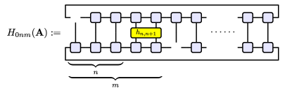
Figure 2: (Color online). Definition of $H_{0nm}({\mathbf{A}})$ as the expectation value of a two-site operator with respect to a TI MPS determined by the tensor ${\mathbf{A}}$.

$H_{eff}(k)$ is constructed very much in the same spirit. First, due to the translational invariance of the Hamiltonian we can write

$$H=\sum_{l=0}^{N-1}h_{l,l+1}=\sum_{l=0}^{N-1}T^{l}h_{01}T^{-l}$$ (8)

where $h_{01}$ is the term acting between the first two sites of the chain. Note that in (8) we have restricted ourselves to nearest neighbor Hamiltonians since this is the type of models we will treat numerically in this work. Generalizing the ideas developed here to any local Hamiltonian is straightforward. With (8), $H_{eff}(k)$ reads

$$\begin{split}&{\mathbf{B}}^{\dagger}H_{eff}(k){\mathbf{B}}=\\ &=\frac{1}{N}\sum_{l,m,n=0}^{N-1}e^{i\frac{2\pi k(n-m)}{N}}\bra{\phi_{\mathbf{A}}({\mathbf{B}})}T^{l-m}h_{01}T^{n-l}\ket{\phi_{\mathbf{A}}({\mathbf{B}})}\\ &=\frac{1}{N}\sum_{l=0}^{N-1}\sum_{\bar{m},\bar{n}=-l}^{N-1-l}e^{i\frac{2\pi k(\bar{n}-\bar{m})}{N}}\bra{\phi_{\mathbf{A}}({\mathbf{B}})}T^{-\bar{m}}h_{01}T^{\bar{n}}\ket{\phi_{\mathbf{A}}({\mathbf{B}})}\,\,\,.\end{split}$$ (9)

Again, due to the fact that the $\bar{m}$ and $\bar{n}$ sums run over all $N$ sites of a PBC chain, it is irrelevant where they begin s.t. the $l$ sum merely yields a factor $N$. We rename the summation indices for convenience and obtain

$$\begin{split}&{\mathbf{B}}^{\dagger}H_{eff}(k){\mathbf{B}}=\\ &=\sum_{m,n=0}^{N-1}e^{i\frac{2\pi k(n-m)}{N}}\bra{\phi_{\mathbf{A}}({\mathbf{B}})}T^{n-m}T^{-n}h_{01}T^{n}\ket{\phi_{\mathbf{A}}({\mathbf{B}})}\\ &=\sum_{n=0}^{N-1}\sum_{\bar{m}=n}^{n-N+1}e^{-i\frac{2\pi k\bar{m}}{N}}\bra{\phi_{\mathbf{A}}({\mathbf{B}})}T^{-\bar{m}}h_{n,n+1}\ket{\phi_{\mathbf{A}}({\mathbf{B}})}\\ &={\mathbf{B}}^{\dagger}\bigg{[}\sum_{m,n=0}^{N-1}e^{-i\frac{2\pi km}{N}}\cdot H_{0nm}({\mathbf{A}})\bigg{]}{\mathbf{B}}\end{split}$$ (10)

where $H_{0nm}({\mathbf{A}})$ is a tensor network resembling the expectation value of an operator acting on the sites $n$ and $n+1$ with respect to a TI MPS where the slots $0$ and $m$ have been left open (see figure 2). The computational cost for the contraction of each tensor network is again $O(D^{6})$ but now we have a total of $N^{2}$ summands s.t. the overall cost for computing $H_{eff}(k)$ is $O(N^{2}D^{6})$. Note that to obtain $H_{eff}(k)$ is computationally the most expensive part of our algorithm so we can say that the overall computational cost scales like $O(N^{2}D^{6})$.

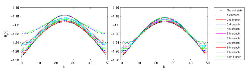
Figure 3: (Color online). Lowest ten branches of the excitation spectrum for a critical Ising chain with $N=50$. Left: $D=8$. Right: $D=32$.

III.1 Overall scaling of the computational cost

At first sight the cost seems horrible for a 1D-algorithm. Let us however have a closer look at what we get for this price. First of all note that if we compute the sets of matrices $\{N_{0m}({\mathbf{A}})\}$ and $\{H_{0nm}({\mathbf{A}})\}$ for $n,m\in[0,N-1]$ and store these, we can obtain the $H_{eff}(k)$ and $N_{eff}(k)$ for all $k$ trivially by just building the appropriately weighted sums. For each of these $k$ we then have to solve the generalized eigenvalue equation (4). Since $H_{eff}(k)$ and $N_{eff}(k)$ are small $dD^{2}\times dD^{2}$ matrices solving (4) does not represent any difficulty and can be done using any standard library eigenvalue solver. Each eigenvalue problem leads to $dD^{2}$ orthonormal vectors ${\mathbf{B}}_{i}(k)$ which plugged into the ansatz (1) yield $dD^{2}$ states. Thus computing the sets $\{N_{0m}({\mathbf{A}})\}$ and $\{H_{0nm}({\mathbf{A}})\}$ only once supplies immediately us with $NdD^{2}$ states! By comparing our numerical results to exactly solvable models we will show that the low energy states obtained in this way are very accurate. This means that in terms of computational time per state our algorithm performs quite well.

The computational bottleneck at the moment is that we have to store $N^{2}$ $dD^{2}\times dD^{2}$ matrices in the memory. With the present implementation, for a chain with $N=100$ sites, we can go up to $D=32$. For larger $N$ simulations we have to settle for smaller $D$. It is however straightforward how this boundary can be pushed considerably towards larger $D$. First, instead of keeping all matrices in the memory, one can write them to the hard disk after computing each of them. Second, since the $\{N_{0m}({\mathbf{A}})\}$ and $\{H_{0nm}({\mathbf{A}})\}$ are independent, one can parallelize their computation.

Thus the conceptual bottleneck becomes the contraction of the tensor networks $\{N_{0m}({\mathbf{A}})\}$ and $\{H_{0nm}({\mathbf{A}})\}$. For non-critical systems big powers of the transfer matrix can be well approximated by a few of its dominant eigenvectors Pirvu et al. (2010a) and the contraction of most of the $\{N_{0m}({\mathbf{A}})\}$ can be done with the computational cost $O(n^{2}D^{3})$ while that of most of the $\{H_{0nm}({\mathbf{A}})\}$ with the cost $O(n^{3}D^{3})$. Here $n$ represents the dimension of the subspace within which we approximate the powers of the transfer matrix Pirvu et al. (2010a). This cannot be done however for critical systems where in principle $n$ may grow as big as $D^{2}$ thereby yielding a much worse scaling than the naive $O(D^{6})$. Note that since $\{N_{0m}({\mathbf{A}})\}$ and $\{H_{0nm}({\mathbf{A}})\}$ are open tensor networks the $O(D^{5})$ contraction scheme Verstraete et al. (2004) that works for expectation values (i.e. closed tensor networks) cannot be applied here. Additionally, even if we restrict ourselves to non-critical systems, not all of the $\{N_{0m}({\mathbf{A}})\}$ and $\{H_{0nm}({\mathbf{A}})\}$ can be computed with the cost that scales like $D^{3}$: if the distance between the open slots is not big enough, we cannot use the approximation for big powers of the transfer matrix between the slots, and we are back to exact contraction for this portion of the chain which in the case of $\{N_{0m}({\mathbf{A}})\}$ leads to the overall scaling $O(nD^{5})$ and in the case of $\{H_{0nm}({\mathbf{A}})\}$ to the scaling $O(n^{2}D^{5})$. Thus the very naive exact contraction procedure that we use is not so bad after all in this case even if it scales like $O(D^{6})$.

There is one more subtlety we would like to point out here. It turns out that the matrix $N_{eff}(k)$ is always singular which presents a problem when we try to solve the generalized eigenvalue equation (4) since the solution involves the inverse $N_{eff}^{-1}(k)$. We can circumvent this problem by solving (4) within the nonsingular subspace like it has been done in Östlund and Rommer (1995). Eigenvectors associated to the zero eigenspace of $N_{eff}(k)$ will result in physical states $\ket{\psi_{k}({\mathbf{B}})}=0$, i.e. these are states of zero length in the Hilbert space. Any physical operator will produce a zero when acting on these states. In particular, the effective Hamiltonian $H_{eff}(k)$ will also have zero eigenvalues for the same eigenvectors, and we do not loose any information by restricting to the nonsingular subspace. The dimension of the zero eigenspace can be shown to be $D^{2}(d-1)$ for $k\neq 0$ and $D^{2}(d-1)+1$ for $k=0$ as we demonstrate in Haegeman et al. (2011). The tricky point is that for some models the strictly non-zero eigenvalues of $N_{eff}(k)$ become so small that they yield the generalized eigenvalue problem ill conditioned. In general this behavior does not occur for small $D$. For big $D$ or in certain regions of the phase diagram however the nonsingular eigenvalues become so small that it is hard to distinguish numerically between the singular subspace and the nonsingular one. This issue might be the source of the mysterious negative gap that appears in Östlund and Rommer (1995) in the vicinity of the critical point.

We have employed a slightly different method for the regularization of $N_{eff}(k)$. Instead of projecting the problem into the strictly non-singular subspace, we restrict ourselves to the subspace in which the eigenvalues of $N_{eff}(k)$ are larger than some $\epsilon$. There is a tradeoff between loss in precision due to this projection and loss in precision due to the bad conditioned generalized eigenvalue problem. In the end we have settled for a seemingly optimal $\epsilon=10^{-11}$.

IV Numerical results

We have applied the algorithm presented above to two exactly solvable nearest neighbour interaction spin models in order to benchmark its accuracy: the quantum Ising model and the Heisenberg spin-$1/2$ antiferromagnetic chain. Even though the Heisenberg model is exactly solvable by means of Bethe ansatz, in practice it is much harder to obtain its entire low-energy spectrum. This is due to the fact that the elementary excitations are two-spinon states and among these, the solution of the Bethe ansatz equations for the two-spinon singlet states are computationally very challenging Karbach et al. (1998). Thus for long chains we have restricted ourselves to check only the precision of the lowest two-spinon triplets. For small chains that are accessible via exact diagonalization on the other hand, we compare not only the entire low-energy spectrum but also the fidelity of the states themselves.

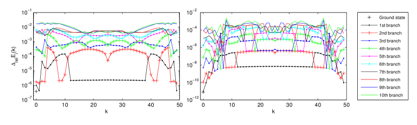
Figure 4: (Color online). Relative precision of the low excitation spectrum for a critical Ising chain with $N=50$. Left: $D=8$. Right: $D=32$.

Table 1: (Color online). Quasi-particle structure of the lowest four branches for $g=1$. The red/blue (grayscale: dark/light) boxes highlight states from the odd-parity subspace respectively from the even parity subspace. The ground state which is not shown in the table is the fermionic vacuum in the even parity subspace i.e. $\ket{GS}=\ket{\Omega}_{even}$.

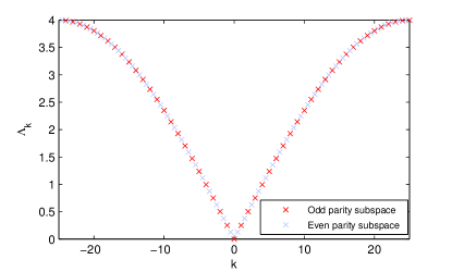
Figure 5: (Color online). Exact solution for the dispersion relation of the Bogoliubov modes at criticality (i.e., $g=1$).

IV.1 Quantum Ising model

The Hamiltonian we have used in our simulations of the Quantum Ising model is given by

$$H_{IS}=-\sum_{i}Z_{i}Z_{i+1}-g\sum_{i}X_{i}\,\,\,.$$ (11)

We have used this version rather than

$$H^{\prime}_{IS}=-\sum_{i}X_{i}X_{i+1}-g\sum_{i}Z_{i}\,\,\,.$$ (12)

due to the fact that having a diagonal interaction term is more convenient for the numerics. Of course both versions are equivalent since they can be transformed into each other by means of the unitary transformation $U=\bigotimes_{i=1}^{N}H_{i}$ where the $H_{i}$ are 1-qubit Hadamard gates. For the exact diagonalization however we have used (12) in order to stick closer to the procedure given in Lieb et al. (1961) where the authors treat the spin-$1/2$ XY chain.

The diagonalization of (12) for PBC in the limit of an infinite number of sites is straightforward Pfeuty (1970). The first thing one has to do is to map the spin Hamiltonian to a fermionic one via a Jordan-Wigner transformation. Now the Jordan-Wigner transformation is non-local due to the fact that it transforms local spin operators into fermionic ones that anticommute if they act on different sites. Luckily for almost all terms in the Hamiltonian the non-localities cancel except for the term representing the interaction between the last and the first site. This term ends up containing a global parity operator acting on all sites and thus breaking the translational invariance with respect to the fermionic modes. Now, if we are interested in the thermodynamic limit, we will eventually take the limes $N\to\infty$ at some point, and in this limit the contribution of one interaction term to the energy can be neglected. We thus have the freedom to alter this term as we please in order to simplify things. One very convenient choice are the so-called Jordan-Wigner boundary conditions which are nothing more than simply neglecting the global parity operator in the last term thereby yielding the fermionic Hamiltonian translationally invariant. Note that the Jordan-Wigner boundary conditions cannot be expressed in a trivial way in terms of spin operators.

The fermionic Hamiltonian obtained in this way is quadratic and translationally invariant, but it is not particle conserving. This can be fixed by a canonical transformation Lieb et al. (1961) to non-interacting Bogoliubov fermions. The ground state of the system is then given by the new fermionic vacuum while excited states can be obtained by sequentially filling the fermionic modes. Ordering the eigenstates of the original spin model by momentum and energy, it turns out that the lowest energy branch coincides with the dispersion relation of the Bogoliubov fermions. This happens because for a given momentum, the lowest energy state is always a state where precisely one fermionic mode is occupied.

Now, for finite systems with periodic boundary conditions, the Hamiltonian after the Jordan-Wigner transformation presents a difficulty: due to the fact that in this case we cannot choose the boundary conditions freely, there is one term that contains a global parity operator as prefactor (see Eq. 2.11’ in Lieb et al. (1961)). At first sight, this term makes the Bogoliubov transformation impossible. However, if we project the Hamiltonian onto the subspaces with either odd or even parity, we can replace the parity operator by its eigenvalue in that subspace s.t. it becomes $\pm 1$, and we can apply the Bogoliubov transformation in each subspace separately. The spectrum of the original Hamiltonian can then be constructed by picking from each subspace the states with the correct parity. It turns out that we can arbitrarily choose the sign of the Bogoliubov parity by shifting the Fermi surface. For example, if we choose the fermionic vacuum to be the state with lowest energy, all excited states are particle excitations and it turns out that the parity operator changes its sign under the Bogoliubov transformation for fields below the critical point i.e. $g<1$. For $g\geq 1$ this choice of the vacuum state leaves the parity operator invariant. Thus for $g<1$, in principle we can switch the sign of the parity operator by shifting the Fermi surface and thereby we could always define the Bogoliubov modes such that the parity operator remains invariant. We will however give numerical evidence for the fact that choosing the Fermi surface to be the fermionic vacuum state is the physical choice.

Let us first present the results obtained at the critical point $g=1$. In Figure 3 we have plotted the energy of the lowest ten branches of excitations of a chain with $50$ spins obtained for MPS bond dimensions $D=8$ and $D=32$. The results for $D=32$ are so close to the exact spectrum that it makes much more sense to look at plots of the relative energy precision rather than at plots of the energy itself. This is shown in Figure 4.

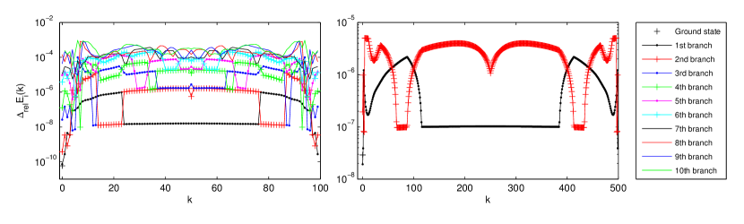
Figure 6: (Color online). Relative precision of the low excitation spectrum for the critical Ising chain with different chain lengths. Left: $N=100$, $D=32$. Right: $N=500$, $D=20$.

At first sight the crossing of the precision line for the first branch of excitations with the one for the second branch seems a little unusual. How can it be that states with higher energy are approximated by roughly two orders of magnitude better than states with lower energy? The answer to this question is obvious if one looks at how the eigenstates emerge from the elementary Bogoliubov modes. Table 1 shows which Bogoliubov modes contribute to each individual eigenstate in the first four branches of excitations. Modes from the even parity subspace have half-integer momentum while the ones from the odd parity subspace have integer momentum. Note that since only excitations with an even number of particles are allowed in the even-parity subspace, the resulting states always have integer momentum. Henceforth $\ket{\Omega}_{even}$ shall denote the vacuum in the even parity subspace and $\ket{\Omega}_{odd}$ the vacuum in the odd parity one. The ground state of the critical chain is the Bogoliubov vacuum in the even parity subspace i.e. $\ket{GS}=\ket{\Omega}_{even}$. The first excited state is the zero momentum state from the first branch and is given by a Bogoliubov mode with zero momentum from the odd parity subspace . It is sufficient to show in Table 1 how the spectrum emerges from elementary excitations for momenta $0\leq k\leq N/2$ since the dispersion relation of the Bogoliubov fermions is symmetric around $k=0$ as can be seen in Figure 5. The important thing to notice in Table 1 is that the lowest branch of excitations does not contain solely one-particle excitations as it does in the case of the infinite chain. Looking back at the right plot in Figure 4 we see immediately that the one-particle excitations from the first two branches are approximated with roughly the same accuracy between $10^{-11}$ and $10^{-9}$ with the lower value for small momentum states. One can easily check that the states with the same order of accuracy from higher branches are precisely one-particle excitations. On the other hand it is obvious that two-particle excitations from any branch where one of the particles has fixed momentum $k=1/2$ can be found in the plateau with relative precision of roughly $10^{-7}$. The other plateaus of similar precision in the $D=32$ plot of Figure 4 represent either two-particle states where each particle has higher momentum or three and more particle excitations.

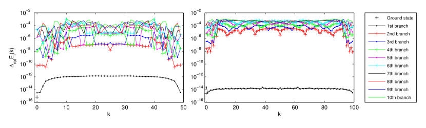
Figure 7: (Color online). Relative precision of the low excitation spectrum for the Ising chain at $g=1.1$ for different chain lengths. Left: $N=50$, $D=32$. Right: $N=100$, $D=32$.

Table 2: (Color online). Quasi-particle structure of the lowest three branches for $g=1.1$. The red/blue (grayscale: dark/light) boxes highlight states from the odd-parity subspace respectively from the even parity subspace. The ground state which is not shown in the table is the fermionic vacuum in the even parity subspace i.e. $\ket{GS}=\ket{\Omega}_{even}$.

This interpretation of the branch crossings in Figure 4 is strong evidence for the fact that (1) is a very good ansatz for one-particle excitations. However it turns out that if $D$ is large enough, (1) is also a fairly good ansatz for many-particle excitations. The reason for this is that the large bond dimension compensates for the localization of excitations inherent in ansatz (1) by spreading the effect of the optimized tensor ${\mathbf{B}}$ to a region around it whose size is of the order of the induced correlation length of the MPS we start with. This is exactly why for the Ising chain with $g=1$, $N=50$ and $D=32$ even states from tenth branch are approximated with an accuracy of roughly $10^{-4}$.

Now let us have a closer look at the region of the ”level-crossing” between the lowest two-fermion branch from the even parity subspace and the lowest one-fermion branch from the odd parity subspace. In the case of $g=1$ this crossing turns out to be at approximately $N/4$. In the immediate neighborhood of the crossing the energy difference between states with identical momentum becomes very small. Now if the bond dimension $D$ is chosen such that the precision of the MPS is of the same order like the interlevel spacing, these two levels cannot be discriminated properly by the MPS algorithm and thus there is no clear interpretation we can give to these MPS states in terms of one or two-particle states. As can be seen in the $D=8$ plot of Figure 4, in this region the first and second MPS branch interpolate between the one and the two-particle states which we can safely discriminate. Note that this observation holds only on the side of the level crossing where the one-particle state has higher energy than the two-particle state (e.g. at $k\approx N/4$ on the left side of the crossing). On the other side, the one-particle excitation has lower energy and our one-particle MPS ansatz is perfectly suited to discriminate between the first and the second branch even if the precision is smaller than the actual gap between the levels.

The last thing we would like point out about Figure 4 is the gap in accuracy between the states from the second and third branch at momentum $k=N/2$. It turns out that this is a doubly degenerate state since it can be created by two different superpositions of elementary excitations with the same energy namely $\ket{\frac{49}{2},\frac{1}{2}}$ and $\ket{-\frac{49}{2},-\frac{1}{2}}$. This is the reason why the precision of the $k=N/2$ state in the second branch is better than that of the surrounding two-particle states which are not degenerated: variational algorithms are more precise if they try to approximate the energy of an entire subspace of the Hilbert space rather than that of a single state. However since all states generated by our algorithm are orthogonal, the price we have to pay for the improved precision in the second branch, is a slightly worse precision of the $k=N/2$ state in the third branch.

With this said, we can present the results we have obtained for different chain lengths $N$ and different values of the magnetic field $g$. Figure 6 shows the accuracy of the algorithm for chains with $100$ and $500$ sites at $g=1$. The plot for $N=100$ is very similar to the $D=32$ plot from Figure 4. At small momenta $6\leq k\leq 11$ the one-particle excitations lie in the branches $4$ to $6$. These states are not reliably reproduced by our algorithm within the precision that is otherwise reached for one-particle excitations. Presumably this would be fixed by increasing the bond dimension $D$ beyond $32$. However at the moment we cannot go to larger $D$ for $N=100$. For $N=500$ the maximally accessible bond dimension is $D=20$. The corresponding plot from Figure 6 is very similar to the small $D$ plot for $N=50$. Again in the region of the ”level-crossing” between one-particle and two-particle excitations around $k=N/4$ our algorithm has difficulties obtaining the maximally reachable precision for the one-particle states.

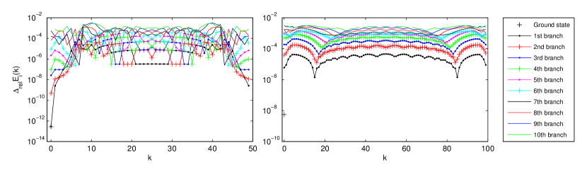
Figure 8: (Color online). Relative precision of the low excitation spectrum for the Ising chain at $g=0.9$ for different chain lengths. Left: $N=50$, $D=32$. Right: $N=100$, $D=32$.

Table 3: (Color online). Quasi-particle structure of the lowest three branches for $g=0.9$. The red/blue (grayscale: dark/light) boxes highlight states from the odd-parity subspace respectively from the even parity subspace. $\ket{\Omega}_{odd}$ denotes the fermionic vacuum in the odd-parity subspace. The ground state which is not shown in the table is the fermionic vacuum in the even parity subspace i.e. $\ket{GS}=\ket{\Omega}_{even}$.

Now let us look at how the algorithm performs when we move away from the critical point. Figure 7 shows the relative energy difference of the MPS approximation for $g=1.1$ i.e. above the critical point. The most striking feature in this regime is clear separation of the lowest branch of excitations from the higher ones. This happens due to the fact that in this case the lowest branch contains only one-particle states as can be seen in Table 2. Again if $D$ is large enough (e.g. $D=32$ for $N=50$), the different plateaus of similar precision become clearly visible. The first one at roughly $\Delta_{rel}E_{i}(k)\approx 10^{-8}$ contains two-particle excitations from the second and third branch where one of the fermionic modes has momentum $k=1/2$. The second one with precision around $10^{-6}$ consists of states where one of the fermionic modes has momentum $k=3/2$. Note that in the plot for $N=100$ the lowest branch has slightly better precision than the one in the $N=50$ plot even though the virtual bond dimension is the same. This happens presumably because in this case the chain is long enough such that the running particle cannot ”feel its own tail” due to the PBC. This is another piece of evidence that ansatz (1) is very well suited to describe one-particle excitations. Whether many-particle excitations are faithfully reproduced depends strongly on the magnitude of $D$ with respect to $N$.

For $g<1$ the picture changes dramatically. We can see in figure 8 that at $g=0.9$ the best precision for states from the lowest branch is five to seven orders of magnitude worse than for $g=1.1$. Without any knowledge of the quasi-particle structure of the spectrum this huge difference might look a bit surprising. Even more surprising is the fact that the best precision at $g=0.9$ is one order of magnitude worse than at the critical point $g=1$. However looking at the quasi-particle structure in Table 3 clarifies the situation. As already mentioned above the parity of the Bogoliubov fermions in the odd-parity subspace can in principle be arbitrarily chosen by shifting the Fermi surface. Throughout this work have made the most natural choice of choosing all modes to have positive energy i.e. none of the quasi-particle excitations are hole modes. For $g<1$ this choice switches the sign of Bogoliubov parity operator such that we must pick states with an even number of excitations from the odd-parity subspace. One might argue against this convention and claim that it would be much more natural to pick the Fermi surface s.t. the zero-momentum mode is a hole excitation which yields the Bogoliubov parity operator identical to the spin parity operator. In this case we would have to construct all states from this subspace using an odd number of quasi-particles. On the other hand Table 3 clearly shows that our one-particle excitation ansatz (1) is a poor approximation to all states in this regime thereby indicating that indeed for $g<1$ there exist no one-particle excitations. Thus our choice of the Fermi surface is justified and we have to construct the spectrum by picking the even quasi-particle excitations from the odd-parity subspace.

We can understand this behavior from another point of view if we consider an infinite chain with open boundary conditions. It is well known that in the region of the phase diagram where the ground state is doubly degenerated, the elementary excitations are kink excitations. If we would however impose periodic boundary conditions on the infinite chain, the single kink states would not be eigenstates any more since the existence of one domain wall would automatically imply the existence of a second one. In finite systems with PBC, the situation is a bit more complicated since the ground state degeneracy is not exact (the energy difference decays exponentially with $N$), but we can still argue along similar lines that localized perturbations, that interpolate between the states of the almost degenerated ground state manifold, must always come in pairs.

IV.2 Heisenberg model

The other model we have studied is the antiferromagnetic (AF) Heisenberg spin-$1/2$ chain. The Hamiltonian reads

$$H_{HB}=\sum_{i=1}^{N}\vec{S}_{i}\vec{S}_{i+1}=\frac{1}{4}\sum_{i=1}^{N}(\sigma^{x}_{i}\sigma^{x}_{i+1}+\sigma^{y}_{i}\sigma^{y}_{i+1}+\sigma^{z}_{i}\sigma^{z}_{i+1})$$ (13)

where $S^{\alpha}=\sigma^{\alpha}/2$ and $\sigma^{\alpha}$ denote as usually the Pauli operators. As we already mentioned, the tensors ${\mathbf{A}}$ that constitute the backbone of ansatz (1) are the results of the simulations presented in Pirvu et al. (2010a). In that work we have obtained a TI MPS approximation of ground states for finite spin chains with PBC using matrices $A_{i}$ that were real and symmetric. These results themselves were based on previous work Pirvu et al. (2010b) where we have approximated the ground state of infinite OBC chains by TI MPS with real symmetric matrices. Thus the starting point in the entire procedure that leads ultimately to the excited states presented here is the imaginary time evolution for an infinite chain with a set of real symmetric matrix product operators (MPO). As we explained in Pirvu et al. (2010b) it is not possible to construct these directly from the the Hamiltonian (13). However, by means of the unitary transformation $U=U^{\dagger}=\prod_{j=1}^{N/2}\sigma^{y}_{2j-1}$ (i.e. acting with a $\sigma^{y}$-gate on every second site) we obtain

$$H^{\prime}_{HB}=U^{\dagger}H_{HB}U=\frac{1}{4}\sum_{i=1}^{N}(-\sigma^{x}_{i}\sigma^{x}_{i+1}+\sigma^{y}_{i}\sigma^{y}_{i+1}-\sigma^{z}_{i}\sigma^{z}_{i+1})$$ (14)

which allows us to express the imaginary time evolution in terms of real symmetric MPO. Note that in order for this procedure to work we have to restrict ourselves to chains with an even number of sites. In this case it does not matter if we apply the $\sigma^{y}$-gates on sites with an odd or an even index, so without loss of generality we will apply them on the odd ones. Now $H_{HB}$ and $H^{\prime}_{HB}$ have the same spectrum and since their eigenstates are simply related to eachother by

$$\ket{\psi_{i}}=\prod_{j=1}^{N/2}\sigma^{y}_{2j-1}\ket{\psi_{i}^{\prime}}$$ (15)

we can digonalize $H^{\prime}_{HB}$ first and obtain the eigenstates of $H_{HB}$ subsequently with very little effort.

Table 4: (Color online). Multiplet structure of the lowest ten branches of excitations for a Heisenberg $16$-site chain with Hamiltonian (13). The colors encode the multiplet information: yellow-singlet, blue-triplet, red-quintuplet, dark red-septuplet (grayscale: darker colors encode higher multiplets). The states within each multiplet are ordered according to their total spin projection quantum number. The sign denotes the parity of a state.

Table 5: (Color online). Multiplet structure of the lowest ten branches of excitations for a Heisenberg $16$-site chain with Hamiltonian (14). The colors encode the multiplet information: yellow-singlet, blue-triplet, red-quintuplet (grayscale: darker colors encode higher multiplets). The sign denotes the parity of a state and the index denotes the momentum $k$ if we apply the transformation (15) to an eigenstate with momentum $k^{\prime}$.

We will show below that the momentum of a state is not always invariant under the transformation (14). The easiest way to obtain the momentum for any given state is by computing the expectation value of the translation operator $T$ with respect to that state. $H_{HB}$ and $H^{\prime}_{HB}$ are both translationally invariant thus all their eigenstates have well defined momentum so we can be sure that the reverse transformation $\ket{\psi_{i}^{\prime}(k^{\prime})}\rightarrow\ket{\psi_{i}(k)}$ will map momentum eigenstates to momentum eigenstates albeit $k$ will generally differ from $k^{\prime}$. The relation between the momenta follows easily from

$$\begin{split}&e^{-i\frac{2\pi k}{N}}=\braket{\psi_{i}(k)}{T}{\psi_{i}(k)}=\\ &=\braket{\psi_{i}^{\prime}(k^{\prime})}{\bigg{(}\prod_{j=1}^{N/2}\sigma^{y}_{2j-1}\bigg{)}T\bigg{(}\prod_{j=1}^{N/2}\sigma^{y}_{2j-1}\bigg{)}}{\psi_{i}^{\prime}(k^{\prime})}\\ &=\braket{\psi_{i}^{\prime}(k^{\prime})}{\bigg{(}\prod_{j=1}^{N/2}\sigma^{y}_{2j-1}\bigg{)}\bigg{(}\prod_{j=1}^{N/2}\sigma^{y}_{2j}\bigg{)}T}{\psi_{i}^{\prime}(k^{\prime})}\\ &=e^{-i\frac{2\pi k^{\prime}}{N}}\braket{\psi_{i}^{\prime}(k^{\prime})}{\prod_{j=1}^{N}\sigma^{y}_{j}\,}{\psi_{i}^{\prime}(k^{\prime})}=e^{-i\frac{2\pi k^{\prime}}{N}}\braket{P_{y}}_{i^{\prime},k^{\prime}}\end{split}$$ (16)

where we have used $T\big{(}\prod_{j}O_{j}\big{)}T^{-1}=\prod_{j}O_{j+1}$ and $T\ket{\psi_{i}^{\prime}(k^{\prime})}=e^{-i\frac{2\pi k^{\prime}}{N}}\ket{\psi_{i}^{\prime}(k^{\prime})}$. Thus the change in momentum depends solely on the expectation value of the operator $P_{y}=\prod_{j=1}^{N}\sigma^{y}_{j}$ which in the following we will call the parity operator. This naming convention makes sense since $P_{y}=i^{N}\exp(i\pi S_{T}^{y})$ where $S_{T}^{y}=\sum_{j=1}^{N}S_{j}^{y}$ thus $P_{y}$ measures the parity of the total spin along the $y$-direction. Note that due to the factor $i^{N}$ the meaning of positive and negative parity is interchanged for chains with $N=0(\mod{4})$ and chains with $N=2(\mod{4})$. The parity is a good quantum number for both $H_{HB}$ and $H_{HB}^{\prime}$ so there exist eigenstates $\ket{\psi_{i}^{\prime}(k^{\prime})}$ that have well defined parity plus or minus one. If $\braket{P_{y}}_{i^{\prime},k^{\prime}}=+1$ the momentum remains unchanged i.e. $k=k^{\prime}$, if $\braket{P_{y}}_{i^{\prime},k^{\prime}}=-1=e^{\pm i\pi}$ we have $k=k^{\prime}\oplus_{N}N/2$ where $\oplus_{N}$ denotes addition modulo $N$. Note that the parity itself is invariant under the mapping between $H_{HB}$ and $H_{HB}^{\prime}$ since $U^{\dagger}P_{y}U=P_{y}$.

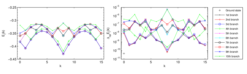
Figure 9: (Color online). Results for the low excitation spectrum (left) and the corresponding relative precision (right) for the Heisenberg spin-$1/2$ chain with $N=16$ sites.

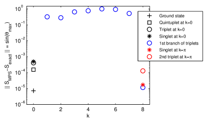
Figure 10: (Color online). Distance between several degenerated subspaces obtained by our algorithm to the corresponding degenerated subspaces obtained by exact diagonalization. As a measure for the distance we have used the sine of the canonical angle with the largest magnitude as defined in Bhatia (1997).

Now the generators of the $SU(2)$ symmetry for $H_{HB}^{\prime}$ do not commute with the translation operator thus we cannot classify the momentum eigenstates in terms of irreducible representations of $SU(2)$. For $H_{HB}$ however we can do this, so we know exactly the degeneracy structure of the spectrum in each subspace with fixed momentum. Thus if we encounter for instance a threefold degenerated eigenstate of $H_{HB}^{\prime}$, we know this is mapped to a spin triplet with well defined momentum in the original Hamiltonian. Accordingly it must contain a two-dimensional subspace with negative parity corresponding to total spin along the $y$-direction $\pm 1$ and a one-dimensional subspace corresponding to total spin $0$. Since the spin triplet in the original Hamiltonian has well defined momentum, according to the rules for the mapping $k\leftrightarrow k^{\prime}$, we will have one eigenstate of $H_{HB}^{\prime}$ with momentum $k$ and a two-dimensional subspace with the same energy but different momentum $k^{\prime}=k\ominus_{N}N/2$. In this way , after approximating the spectrum of $H_{HB}^{\prime}$ and labeling all energies with the corresponding momentum we can obtain the spectrum of $H_{HB}$ by mere inspection of the degeneracy structure. Table 4 and Table 5 illustrate how the multiplets of $H_{HB}$ and $H_{HB}^{\prime}$ are related to eachother.

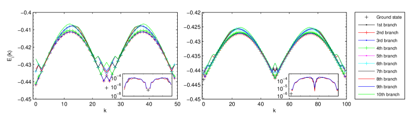
Figure 11: (Color online). Results for the low excitation spectrum and the corresponding relative precision of the lowest triplet (insets) for the Heisenberg spin-$1/2$ chain with $N=50$ (left) and $N=100$ (right) sites.

This procedure works very well for the lower branches of the dispersion relation where the precision of our simulation is good enough to discriminate unambigously between different multiplets. For higher branches, on one hand the precision gets worse and on the other hand the density of states increases such that multiplets with similar energy become effectively undistiguishable for our algorithm. In this case the eigenstates with well defined momentum that we obtain for the Hamiltonian $H_{HB}^{\prime}$ do not have well defined parity i.e. they mix parity eigenstates with different parity. Since states with same momentum and different parity are mapped by (15) to states with different momentum, if we start with such a momentum eigenstate we obtain after the transformation a superposition of states with different momenta which is clearly not a momentum eigenstate. There are however two ways to overcome this issue and obtain approximations of the eigenstates of $H_{HB}$ that are at the same time exact momentum eigenstates.

The first one amounts to computing the matrix elements of the translation operator $T$ in the subspace spanned by the transformed states $\{M_{odd}^{y}\ket{\psi_{i}^{\prime}(k)^{\prime}}\}$ where $M_{odd}^{y}:=\prod_{j=1}^{N/2}\sigma_{2j-1}^{y}$ and then diagonalize this matrix. It is not difficult to check that this can be done for each momentum $k^{\prime}$ separately since $M_{odd}^{y}\,T\,M_{odd}^{y}=M_{odd}^{y}\,M_{even}^{y}\,T=P_{y}T$ which is a translationally invariant operator and thus it does not mix states with different momentum. Diagonalizing each of the $T(k^{\prime})_{ij}=U^{\dagger}(k^{\prime})_{il}D(k^{\prime})_{lm}U(k^{\prime})_{mj}$ yields for each $k^{\prime}$ a unitary $U(k^{\prime})$ that is nothing more than the transformation that we need to obtain the desired momentum eigenstates via $\ket{\psi_{i}(k_{i})}=U(k^{\prime})_{ij}\ket{\psi_{j}^{\prime}(k^{\prime})}$. The new momentum $k_{i}$ can be read off the diagonal matrix $D(k^{\prime})$. There are two drawbacks that come with this procedure. The first one is that we must compute the matrix elements $T(k^{\prime})_{ij}$ each of which is done with the computational cost $O(ND^{5})$. Since there are $Nb^{2}$ of these where $b$ is the number of branches, we obtain the overall cost $O(N^{2}b^{2}D^{5})$. Usually we compute enough branches such that $b^{2}>D$ holds, thus the cost for this procedure ends up being higher than the one for the diagonalization of $H_{HB}^{\prime}$. The second drawback is that the superpositions $U(k^{\prime})_{ij}\ket{\psi_{j}^{\prime}(k^{\prime})}$ mix the original approximations of the energy levels thereby slightly lowering the energy of higher excitations but increasing the energy of lower excitations, which are usually the ones we are most interested in.

The second way to approximate the eigenstates of the original Hamiltonian $H_{HB}$ such that they are at the same time exact momentum eigenstates is to add to $H_{HB}^{\prime}$ a perturbation that splits degenerated levels with different parity. This is easily achieved by taking $H_{HB}^{\pm}:=H_{HB}^{\prime}\pm\lambda P_{y}$ where $\lambda$ must be chosen such that it is big enough for our algorithm to deliver only states with a single parity, but as small as possible in order to avoid numerical inaccuracies caused by altering the Hamiltonian. In the case of the Heisenberg model, if we choose to compute $b=10$ branches, $\lambda=0.1\cdot N$ fulfills these requirements. In practice we first apply our algorithm to $H_{HB}^{-}$ which yields for each momentum $k^{\prime}$ $b$ states with positive parity. These states do not change their momentum under the transformation (15). Subsequently we apply the algorithm to $H_{HB}^{+}$ which yields states with negative parity that change their momentum after the transformation according to $k=k^{\prime}\oplus_{N}N/2$. In this way we end up with $2b$ branches of states that approximate the spectrum of $H_{HB}$ and that are at the same time exact momentum eigenstates. The computational cost per state is thus exactly the same like diagonalizing only $H_{HB}^{\prime}$.

Let us first look at the results we have obtained for a small chain with $16$ sites. We have chosen to look at such a small system first for two reasons: First, even though the Heisenberg model is exactly solvable via Bethe ansatz, obtaining all energy levels can be quite involved. Choosing $N$ as small as $16$ allows us to compute the spectrum of this small chain by means of exact diagonalization. Second, even for the energy levels that are easily computable with the Bethe ansatz (i.e., the triplet states in the subspace of two-spinon excitations Karbach et al. (1998)) it is not possible to obtain the eigenstates themselves. Exact diagonalization of a small chain on the other hand allows us to compute and store the exact eigenstates in order to check the fidelity of our MPS approximation.

Figure 9 shows the energy of the first ten branches of excitations and the corresponding relative precision. Note how states belonging to the same multiplet have very similar precision even though they have different parity and thus correspond to eigenstates of $H_{HB}^{\prime}$ with different momentum. Since there are no one-particle excitations in the low-energy spectrum of the AF Heisenberg model, we do not obtain such a good precision like in the case of the quantum Ising model. Nevertheless we get a very good approximation of the first excited level, namely the triplet excitation at $k=N/2$. We have also tested the accuracy of the states themselves: for non-degenerated states, the absolute value of the overlap is a perfect measure for this, and for reasons that will become clear immediately, we have looked at the sine of the fidelity. For degenerated states, in order to compare the subspace spanned by our MPS to the one spanned by the exact eigenstates, we have used as a measure for the distance the definition given in chapter 7 of Bhatia (1997): the sine of the largest canonical angle between the two subspaces. The canonical angles can be easily computed from the matrix that has as its entries the overlaps between all states of the subspaces that we want to compare. The results are plotted in figure 10. We see that only the MPS with momentum $k=0$ and $k=N/2$ are extremely accurate. All other states, especially those around $k=N/4$, are much further away from the exact solutions, which is a bit surprising given the fact that the energy precision for these states is comparable to the one obtained for $k=0$.

The spectrum that we obtain for longer chains is plotted in figure 11. In this regime we have only looked at the precision of the lowest two-spinon triplet for which the exact results were obtained following Karbach et al. (1998). Again we see that the states at momentum $k=k_{0}\oplus N/2$ have the best accuracy. We would like to make two more remarks concerning the chain with $N=50$. First, note that the ground state has momentum $k_{0}=N/2$ in this case. Second, unlike in the case of $N=100$, where for all momenta $k\neq k_{0}$ the lowest excitation is a triplet, we observe that for $N=50$ this does not happen. Our simulations reveal that at $k\in\{2,3,47,48\}$ the quintuplet excitation lies below the triplet while at $k\in\{23,27\}$ it is a singlet that is the lowest lying excitation.

V Conclusions and Outlook

Inspired by previous approaches Östlund and Rommer (1995); Porras et al. (2006) we have introduced a new method for the simulation of translationally invariant spin chains with periodic boundary conditions. We have used an MPS based ansatz that corresponds to a particle-like excitation with well defined momentum in order to obtain extremely accurate results for models where the spectrum contains precisely one-particle states. For states that can be expressed in terms of many quasi-particle excitations, we still obtain feasible results if the MPS bond dimension is chosen to be big enough. In the case of the quantum Ising model, our results indicate that for $g<1$ the spectrum is built up entirely out of excitations with an even number of quasi-particles. Generalizations of our approach can go in two directions: First, it is possible to adjust ansatz (1) in order to treat infinite systems with open boundary condition, which we are addressing in Haegeman et al. (2011). Second, it seems feasible to generalize our approach to a many-particle ansatz by using more than one MPS tensor in (1) in order to define the variational manifold.

VI Acknowledgements

We thank G.Vidal, V. Murg, E. Rico and B. Nachtergaele for valuable discussions. This work was supported by the FWF doctoral program Complex Quantum Systems (W1210), the Research Foundation Flanders, the ERC grant QUERG, and the FWF SFB grants FoQuS and ViCoM.

References

- Östlund and Rommer (1995) S. Östlund and S. Rommer, Phys. Rev. Lett. 75, 3537 (1995)
- Rommer and Östlund (1997) S. Rommer and S. Östlund, Phys. Rev. B 55, 2164 (1997)
- Pirvu et al. (2010a) B. Pirvu, F. Verstraete, and G. Vidal (2010a), eprint arXiv:1005.5195
- Porras et al. (2006) D. Porras, F. Verstraete, and J. I. Cirac, Phys. Rev. B 73, 014410 (2006)
- Verstraete et al. (2004) F. Verstraete, D. Porras, and J. I. Cirac, Phys. Rev. Lett. 93, 227205 (2004)
- Fannes et al. (1992) M. Fannes, B. Nachtergaele, and R. Werner, Communications in Mathematical Physics 144, 443 (1992), ISSN 0010-3616, 10.1007/BF02099178, URL http://dx.doi.org/10.1007/BF02099178
- Chung and Wang (2009) S. G. Chung and L. Wang, Physics Letters A 373, 2277 (2009), ISSN 0375-9601
- Haegeman et al. (2011) J. Haegeman, B. Pirvu, D. Weir, J. Cirac, T. Osborne, H. Verschelde, and F. Verstraete (2011), eprint arXiv:1103.2286
- Karbach et al. (1998) M. Karbach, K. Hu, and M. Gerhard, Comp. in Phys. 12, 565 (1998), eprint arXiv:cond-mat/9809163
- Lieb et al. (1961) E. Lieb, T. Schultz, and D. Mattis, Annals of Physics 16, 407 (1961)
- Pfeuty (1970) P. Pfeuty, Annals of Physics 57, 79 (1970), ISSN 0003-4916
- Not (a) If the fermionic vacuum is not the lowest energy state there also exist hole and particle-hole excitations. If we choose the vaccum in such a way that there exists exactly one hole-mode we effecively switch the sign of the parity operator opposed to choosing no hole-modes at all.
- Not (b) Actually at the zero momentum mode has energy zero so the states and have exactly the same energy. However this happens only at the critical point . In general and have different energy.
- Pirvu et al. (2010b) B. Pirvu, V. Murg, J. I. Cirac, and F. Verstraete, New J. Phys. 12, 025012 (2010b)
- Bhatia (1997) R. Bhatia, Matrix analysis (Springer-Verlag New York, 1997)
- Not (c) A singlet state would have parity and thus there would be no momentum shift in this case. A quintuplet would contain a three-dimensional subspace with parity and a two-dimensional subspace with parity . Thus in this case we would observe three states with no momentum shift and two states with a -shift. The generalization to higher multiplets is obvious.