Quantitative study of quasi-one-dimensional Bose gas experiments via the stochastic Gross-Pitaevskii equation

Abstract

The stochastic Gross-Pitaevskii equation is shown to be an excellent model for quasi-one-dimensional Bose gas experiments, accurately reproducing the in situ density profiles recently obtained in the experiments of Trebbia et al. [Phys. Rev. Lett. 97, 250403 (2006)] and van Amerongen et al. [Phys. Rev. Lett. 100, 090402 (2008)], and the density fluctuation data reported by Armijo et al. [Phys. Rev. Lett. 105, 230402 (2010)]. To facilitate such agreement, we propose and implement a quasi-one-dimensional stochastic equation for the low-energy, axial modes, while atoms in excited transverse modes are treated as independent ideal Bose gases.

I Introduction

Ultracold atomic gases are proving to be extremely useful tools for synthesizing low dimensional quantum models owing to the huge degree of controlability they offer Bloch et al. (2008). The effective system dimensionality may be tuned in experiments by manipulation of external trapping potentials, with the underlying physics ultimately set by the trap geometry and level of quantum degeneracy Görlitz et al. (2001). Increasing the trapping potential in one direction leads to an effectively two-dimensional (2D) system Görlitz et al. (2001); Rychtarik et al. (2004); Stock et al. (2005); Smith et al. (2005), which allows access to a number of interesting phenomena such as the Berezinskii-Kosterlitz-Thouless transition and related studies on the nature of the Bose gas in two-dimensions Hadzibabic et al. (2006); Schweikhard et al. (2007); Krüger et al. (2007); Hadzibabic et al. (2008); Cladé et al. (2009); Rath et al. (2010); Tung et al. (2010); Hung et al. (2011). Increasing the trapping potential in a further direction results instead in an effectively one-dimensional (1D) system Moritz et al. (2003); Paredes et al. (2004); Kinoshita et al. (2004); Cacciapuoti et al. (2003); Trebbia et al. (2006); van Amerongen et al. (2008); Armijo et al. (2010, 2011); Estève et al. (2006); Dettmer et al. (2001); Hellweg et al. (2003); Gerbier et al. (2003); Richard et al. (2003); Manz et al. (2010); Gustavson et al. (1997); Hinds et al. (2001); Schumm et al. (2005); Hofferberth et al. (2006); Fixler et al. (2007); Jo et al. (2007); Hofferberth et al. (2007); Gross et al. (2010); Baumgärtner et al. (2010); Hinds and Hughes (1999); Ott et al. (2001); Hänsel et al. (2001); Folman et al. (2002); Fortágh and Zimmermann (2007); Reichel and Vuletic (2011).

In a 1D set-up, one may obtain Petrov et al. (2000) either a weakly-interacting system, or, for rather low densities, a strongly-interacting Tonks-Girardeau gas Girardeau (1960); Moritz et al. (2003); Paredes et al. (2004); Kinoshita et al. (2004). The finite temperature phase diagram of a weakly interacting 1D Bose gas Petrov et al. (2000); Al Khawaja et al. (2003); Armijo et al. (2011) is more complex than that of a 3D gas, due to a separation in the temperatures for the onset of density and phase fluctuations. Density fluctuations are typically suppressed at higher temperatures than phase fluctuations, allowing for the formation of a so-called quasi-condensate Popov (1983).

\psfrag{yaxis}{\scalebox{3.75}{$k_{B}T/\hbar\omega_{\perp}$}}\psfrag{xaxis}{\scalebox{3.75}{$\mu/\hbar\omega_{\perp}$}}\includegraphics[angle={0},scale={0.3},clip]{Cockburn_etal_fig1.eps}

Figure 1: (Color online) Phase diagram indicating the theoretically obtained parameters for the experiments considered. Hollow symbols indicate density profile data of Trebbia et al. (2006) and van Amerongen et al. (2008), whereas filled symbols indicate the density fluctuation data of Armijo et al. (2010).

A number of experiments have recently probed the physics of highly-elongated finite temperature Bose gases at equilibrium, including the direct observation and analysis of density Cacciapuoti et al. (2003); Estève et al. (2006); Armijo et al. (2010) and phase fluctuations Dettmer et al. (2001); Hellweg et al. (2003); Gerbier et al. (2003); Richard et al. (2003); Manz et al. (2010). Understanding the properties of matter waves in such geometries is of key importance to atom interferometers Gustavson et al. (1997); Hinds et al. (2001); Schumm et al. (2005); Fixler et al. (2007); Jo et al. (2007); Hofferberth et al. (2007); Gross et al. (2010); Baumgärtner et al. (2010) and atom chips Hinds and Hughes (1999); Hänsel et al. (2001); Ott et al. (2001); Folman et al. (2002); Hofferberth et al. (2006); Fortágh and Zimmermann (2007); Reichel and Vuletic (2011).

In this paper, we show that in situ density profiles and density fluctuations from the elongated Bose gas experiments of Trebbia et al.Trebbia et al. (2006), van Amerongen et al.van Amerongen et al. (2008), and Armijo et al.Armijo et al. (2010), can be predicted ab initio by means of an effective 1D stochastic model; to achieve this, we propose and implement for the first time a modification to the usual form of the stochastic Gross-Pitaevskii equation Stoof (1999); Stoof and Bijlsma (2001); Gardiner and Davis (2003) which additionally incorporates quasi-1D effects. Such an extension beyond the purely 1D limit is required, since these experiments probe regimes for which both $\mu,\,k_{B}T\gtrsim\hbar\omega_{\perp}$, as evident from Fig.1. Thus, one should in general account for both a quasi-1D degenerate system exhibiting fluctuations and for the non-negligible role of transverse thermal modes. These are included here by (i) implementing a stochastic quasi-1D equation of state for the axial modes, and (ii) treating atoms in excited transverse modes as independent, ideal Bose gases, as proposed in a related study van Amerongen et al. (2008).

In Sec. II we discuss our methodology in more detail, while Sec. III focuses on the ab initio reproduction of the experimental density profiles and density fluctuation results reported in Trebbia et al. (2006); van Amerongen et al. (2008); Armijo et al. (2010), with our conclusions presented in Sec. IV.

II Methodology

We seek a model which can provide ab initio predictions for experimentally measurable properties obtained by in situ absorption imaging. There are two issues that need to be addressed simultaneously here, regarding the spatial extent of the quasi-condensate in the transverse direction, and the role of atoms in excited transverse modes. As mentioned, the important parameters affecting these are the ratio of the chemical potential, $\mu$, and thermal energy, $k_{B}T$, to the transverse ground state energy $\hbar\omega_{\perp}$. For $\mu\ll\hbar\omega_{\perp}$, the transverse ground state density has a Gaussian profile of width $l_{\perp}$, the transverse oscillator length, whereas for larger $\mu$, this width becomes increased due to the effect of repulsive interactions. On the other hand, if $k_{B}T\ll\hbar\omega_{\perp}$, then thermal occupation of the transverse excited modes is negligibly small; for higher temperatures, this is no longer true and atoms in these modes will contribute considerably to experimental observables, such as density profiles.

In the present work, we treat the quasi-condensate and thermal modes separately: consideration of transverse thermal modes is crucial for matching total atom numbers and density profiles, however they may be simply and accurately described as independent equilibrium Bose gases, as shown in van Amerongen et al. (2008); fluctuating axial modes are instead treated within our modified stochastic model, a novel feature of this work, which is discussed in detail below.

Quasi-condensate Modeling - The axial modes of a sufficiently elongated Bose gas are typically subject to phase and density fluctuations due to thermal excitations with wavelengths greater than the radial extent of the gas Stringari (1998); Petrov et al. (2001). This requires the inclusion of such fluctuations when describing modes with energies less than $\hbar\omega_{\perp}$. We therefore choose to describe these axial modes dynamically using a stochastic Gross-Pitaevskii equation (SGPE) Stoof (1999); Stoof and Bijlsma (2001); Gardiner and Davis (2003). In solving this equation, we make the following two assumptions: (i) thermal modes (with energies $>\hbar\omega_{\perp}$) may be treated as though at equilibrium, and therefore represent a heat bath in contact with the axial sub-system (these two components are assumed to be in diffusive and thermal equilibrium with a temperature $T$ and chemical potential $\mu$); (ii) the modes in the weakly trapped, axial direction are sufficiently highly occupied that the classical field approximation is valid Svistunov (1991); Stoof and Bijlsma (2001); Duine and Stoof (2001); Davis et al. (2001); Sinatra et al. (2001); Goral et al. (2001).

Under assumptions (i) and (ii), the axial modes may be represented by the 1D SGPE,

$$\begin{split}i\hbar\frac{\partial\psi(z,t)}{\partial t}&=(1-i\gamma(z,t))\bigg{[}-\frac{\hbar^{2}}{2m}\frac{\partial^{2}}{\partial z^{2}}+V(z)\\ &+g|\psi|^{2}-\mu\bigg{]}\psi(z,t)+\eta(z,t),\end{split}$$ (1)

where $\psi$ is a complex order parameter, $V(z)=m\omega_{z}^{2}z^{2}/2$ is the axial trapping potential, $g=2\hbar\omega_{\perp}a$ is the one-dimensional interaction strength (with $a$ the s-wave scattering length), and $\eta$ is a complex Gaussian noise term, with correlations given by the relation $\langle\eta^{*}(z,t)\eta(z^{\prime},t^{\prime})\rangle=2\hbar\gamma(z,t)k_{B}T\delta(z-z^{\prime})\delta(t-t^{\prime})$. The strength of the noise, and damping, due to contact with the transverse thermal modes, is given by $\gamma(z,t)$. This may be calculated ab initio in terms of the Keldysh self-energy Stoof (1999); Stoof and Bijlsma (2001); Duine and Stoof (2001), however as we are interested only in the system properties at equilibrium, we may approximate this quantity to be spatially and temporally constant . To a good approximation, this is given by $\gamma=3\times 4ma^{2}k_{B}T/(\pi\hbar^{2})$ Penckwitt et al. (2002); Duine et al. (2004).

Eq.(1) is valid in the scenario that the transverse ground state is a Gaussian of width $l_{\perp}$. However, as we wish to consider experimental data from actual quasi-1D systems, we should additionally modify our model in a manner which accounts for the transverse swelling of the Bose gas due to repulsive interactions, as seen experimentally Krüger et al. (2010). In the context of the ordinary Gross-Pitaevskii equation, one may replace the 1D equation of state $\mu[n]=gn$, where $n$ denotes the density, with Fuchs et al. (2003)

$$\mu[n]=\hbar\omega_{\perp}\left[\sqrt{1+4na}-1\right],$$ (2)

which is obtained variationally by minimising the 3D GPE with respect to the transverse chemical potential Gerbier (2004); Muñoz Mateo and Delgado (2007); Frantzeskakis (2010). This was shown in Gerbier (2004) to interpolate smoothly across the 1D-to-3D crossover Menotti and Stringari (2002), and reduces to the 1D result in the limit that $4an\ll 1$, as pointed out (for the ordinary GPE) in Fuchs et al. (2003); Muñoz Mateo and Delgado (2007); Frantzeskakis (2010).

Motivated by this we propose, somewhat heuristically, a similar amendment to the 1D stochastic equation (Eq.(1)); for elongated but not truly 1D atomic clouds, this gives rise to the modified stochastic equation

$$\begin{split}i\hbar&\frac{\partial\psi(z,t)}{\partial t}=(1-i\gamma(z,t))\bigg{[}-\frac{\hbar^{2}}{2m}\frac{\partial^{2}}{\partial z^{2}}+V(z)\\ &+\hbar\omega_{\perp}\left(\sqrt{1+4a|\psi|^{2}}-1\right)-\mu\bigg{]}\psi(z,t)+\eta(z,t)\;,\end{split}$$ (3)

which we henceforth refer to as the quasi-1D SGPE. The proposed modification to the 1D SGPE is likely to become important when the inequality $\mu\ll\hbar\omega_{\perp}$ is no longer satisfied, signaling the onset of quasi-1D effects. This method is of course only intended for modeling very elongated systems with $\mu\lesssim{\rm few}\leavevmode\nobreak\ \hbar\omega_{\perp}$, in the weakly-interacting regime $mg/\hbar^{2}n\ll 1$; in this work we thus restrict the application of this equation to the weakly interacting regime, where numerous experiments exist.

In our stochastic scheme, the equilibrium state is reached in a dynamical manner, when the effects of the noise and damping terms of Eq.(3) balance out. Although we demonstrate that this leads to accurate equilibrium predictions, the validity of this equation for describing dynamical features remains to be investigated.

Thermal Transverse Modes: Atoms in the transverse modes are considered to be in static equilibrium, distributed according to Bose-Einstein statistics; the relative importance of their contributions depends on the ratio $k_{B}T/\hbar\omega_{\perp}$, and their contribution is significant in most experimentally relevant cases Trebbia et al. (2006); van Amerongen et al. (2008); Armijo et al. (2010) (except at extremely low temperatures). To account for their contribution to total linear density profiles, we compute (making the $\mu$ and $T$ dependence explicit for clarity)

$$n(z;\mu,T)=\langle|\psi(z;\mu,T)|^{2}\rangle+n_{\perp}(z;\mu,T)$$ (4)

where

$$n_{\perp}(z;\mu,T)=\frac{1}{\lambda_{\rm dB}}\sum_{j=1}^{\infty}(j+1){\rm g}_{1/2}\left[e^{(\mu-V(z)-j\hbar\omega_{\perp})/k_{B}T}\right],$$ (5)

${\rm g}_{1/2}[\ldots]$ is the polylogarithm (or Bose function) of order $1/2$, and $\lambda_{\rm dB}=h/\sqrt{2\pi mk_{B}T}$ is the thermal de Broglie wavelength.

Such an addition of particles in thermal modes has already been used in the so-called modified Yang-Yang model of van Amerongen et al. (2008), where Eq. (5) was used in conjunction with a description of atoms within axial modes based on Yang-Yang theory. In our approach, we effectively replace the Yang-Yang theory with the SGPE, thereby also providing an indirect comparison between SGPE and Yang-Yang, in the weakly-interacting limit. Furthermore, on making this replacement, the contribution given by $n_{\perp}$ remains consistent with our treatment of bosons in excited transverse modes as having already reached thermal equilibrium, as assumed within the SGPE model we apply here.

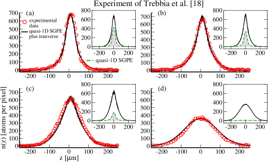
Figure 2: (Color online) Total linear density profiles from the quasi-1D SGPE model (Eq.(4); black solid line) versus data from the experiment of Trebbia et al.Trebbia et al. (2006) (red circles). Insets: quasi-1D SGPE contribution (Eq.(3); green dashed shaded region) to the total linear density profiles (Eq.(4); black solid line). Bottom: Table showing parameters $\mu$ and $T$ for the quasi-1D SGPE density profiles which match the experimental data; the parameters given in Trebbia et al. (2006) from a 3D Hartree-Fock fit are also shown.

To summarize briefly, our approach for modeling equilibrium properties of finite temperature quasi-1D Bose gases is based on self-consistently solving Eq.(3) and Eq.(5) for the desired total atom number (or measured peak density) and temperature .

In Sections III.1 and III.2, we give a quantitative comparison between the proposed method and published in situ experimental data, thereby highlighting the usefulness of this method. For a direct comparison to these experiments, we choose here to fix the temperature to that reported in the experimental papers, and then use $\mu$ as a free parameter, which we vary until the required linear density is obtained at the trap centre.

III Comparison to Experiments

III.1 Density Profiles

We begin with a comparison of the model to total linear density profiles, as obtained by in situ absorption imaging within two experiments: Sec. III.1 gives a comparison to the data of Trebbia et al.Trebbia et al. (2006), whose published analysis was based on a 3D Hartee-Fock model, before discussing the measurements of van Amerongen et al.van Amerongen et al. (2008), who instead analyzed their results via the modified Yang-Yang theory.

In each study, experimental data was compared to theory in order to quantify the equilibrium state through a chemical potential and temperature. The temperature may be quite straight-forwardly measured by fitting the wings of the density distribution to the ideal gas result (for sufficiently high temperatures), implying interactions have little effect on measurements of this parameter. Conversely, the chemical potential is far more dependent on the model used in analyzing the density profile; this is because different theories represent the full quantum Hamiltonian of the interacting system to different levels of approximation (see e.g. Proukakis and Jackson (2008)), so incorporate many-body effects to a differing degree.

It is worth pointing out also, that the density profiles of the theory presented here, and those from experimental absorption imaging share a common feature: namely, that additional analysis is required to identify a phase coherent (or ‘true’ condensate) and density coherent (or quasi-condensate) fraction from the total density. In the SGPE, the total density is due to both coherent and incoherent particles, however knowledge of the first and second order correlation functions was shown to be sufficient to isolate both quasi-condensate and true-condensate densities Cockburn et al. (2010); Wright et al. (2010). In particular, the method discussed in Cockburn et al. (2010) may be easily applied to directly extract such components from experimental measurements of correlation functions, thereby offering a more accurate, experimentally self-consistent, characterisation of phase-fluctuating experiments (without the need to resort to bimodal fits which become somewhat inaccurate in this limit).

III.1.1 Comparison to work of Trebbia et al. Trebbia et al. (2006)

The results of Trebbia et al. demonstrated experimentally the breakdown of the Hartree-Fock method when applied to highly elongated Bose gases Trebbia et al. (2006). It was concluded that this breakdown occurs because density fluctuations are not accounted for accurately within this theory, since the energy lowering effect of spatial correlations between atoms is not captured. These density correlations Naraschewski and Glauber (1999); Prokof’ev and Svistunov (2002); Proukakis (2006); Bisset and Blakie (2009) are key to correctly predicting the onset of quasi-condensation and the associated reduction in density fluctuations; it was found, therefore, that the excited states did not saturate within Hartree-Fock theory and so no quasi-condensate was predicted to form.

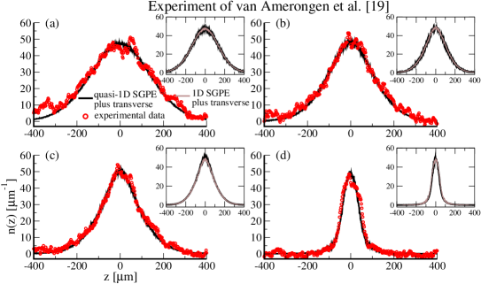
Figure 3: (Color online) Top: Total linear density profiles from the quasi-1D SGPE (black solid line) versus the experimental data of van Amerongen et al.van Amerongen et al. (2008) (red circles). Insets: Quasi-1D SGPE (thick black line) versus 1D SGPE (thin brown line) density profiles. Bottom: Table showing parameters $\mu$ and $T$ for the 1D and quasi-1D SGPE density profiles which match the experimental data and modified Yang-Yang model fits from van Amerongen et al. (2008).

If we compare instead to the results of the quasi-1D SGPE, with the total linear density given by Eq. (4), we see from Fig.II that the theoretical results (black solid line) match well those obtained within the experiments (red circles). The agreement is extremely good across the entire range of temperatures considered, notably even at a temperature close to the crossover from quasi-condensate to thermal gas (Fig. II(c)). It is precisely this regime of critical fluctuations in which a deviation from mean field theory might be expected, due to the lack of a well defined mean field quantity. Interestingly, behaviour suggestive of this was found in Trebbia et al. (2006) when comparing their data to the Hartree-Fock mean field model: the experimental data was found to have a higher peak than the mean field result [see Fig1(c) of Trebbia et al. (2006)], which illustrates the potential importance of including many-body effects, as studied recently in the context of a finite-temperature classical field theory Wright et al. (2010).

We obtain a good fit between the quasi-1D SGPE and experimental density profiles, at the experimentally measured temperatures, with a comparison between the chemical potentials extracted in our treatment and the published values based on the Hartree-Fock analysis of Trebbia et al. (2006) shown in the table . The deviation between the parameters of different theoretical methods should not be of any concern, as it merely highlights $\mu$ as a model dependent quantity, i.e. it is dependent on the actual Hamiltonian used to analyse the experimental results, and therefore varies depending upon the level of approximation Wright et al. (2010); Cockburn et al. (2010).

The insets of Fig.II show the contributions to the total linear density profiles due to the axial SGPE density (green dashed, shaded region), with the remainder coming from Eq.(5). The importance of the SGPE contribution is clear in the first three plots, which shows an appreciable fraction of atoms reside in axial modes for these parameters. In the highest temperature case, shown in Fig.II(d), $\mu<0$ and the gas is entirely in the thermal phase; here the density is instead due almost entirely to atoms in tranverse modes.

III.1.2 Comparison to work of van Amerongen et al. van Amerongen et al. (2008)

The second experiment that we consider is that of van Amerongen et al. van Amerongen et al. (2008). This was the first experimental comparison to the exact Yang-Yang thermodynamic solution to the finite temperature 1D Bose gas problem Yang and Yang (1969), also referred to as the thermodynamic Bethe ansatz.

In van Amerongen et al. (2008), the one-dimensional Yang-Yang theory was used to represent the axial modes and transverse ground state (of width $l_{\perp}$), while the contribution to the linear density due to atoms in transverse excited states, was accounted for using the method we also adopt here. The total density profiles in van Amerongen et al. (2008) were therefore calculated using Eq.(4), with the role of the SGPE contribution $\langle|\psi|^{2}\rangle$ instead played by the 1D Yang-Yang prediction. Therefore, in comparing to this work, we will gain insight on two fronts: firstly, how well the SGPE matches the experimental data in this regime, and simultaneously (but indirectly), how well the SGPE prediction for the density profiles matches that due to Yang-Yang thermodynamics.

Fig.II shows that the agreement between the experimental data and the proposed quasi-1D SGPE approach is again very good across the entire temperature range probed, including the crossover from quasi-condensate to degenerate thermal gas.

We now wish to discuss how our quasi-1D SGPE results compare to those from the SGPE with the usual 1D equation of state. Practically, this means using the equilibrium result of Eq. (1), rather than Eq. (3), as the axial density input $\langle|\psi|^{2}\rangle$ in Eq. (4). Although this approach also recovers closely the total density profiles found with the quasi-1D SGPE at each temperature (insets to Fig. II), and therefore also those measured experimentally, it is important to note that each approach can lead to slightly different chemical potentials for the same temperature.

Importantly, we find that the parameters used to obtain the 1D SGPE results are identical to those obtained from fits of the modified Yang-Yang model to the density data in van Amerongen et al. (2008). These results have also been reported Kheruntsyan et al. (2010) to arise within the context of the closely-related 1D stochastic projected Gross-Pitaevskii equation (SPGPE) Blakie et al. (2008) in parallel independent work, which also looked at the momentum distribution of the gas after focussing Shvarchuck et al. (2002). This provides an indirect additional test between the 1D SGPE, the 1D SPGPE and Yang-Yang theories in the weakly-interacting regime. The parameters predicted by the quasi-1D SGPE, 1D SGPE and modified Yang-Yang models are shown in the Table of Fig.II.

Having established that both the 1D and quasi-1D SGPE approaches accurately reproduce experimental density profiles (and therefore also those due to the modified Yang-Yang approach used in van Amerongen et al. (2008)), we now turn to an investigation of density fluctuations, which provide a more sensitive probe for the validity of these theories.

III.2 Density fluctuations

Density fluctuations are increased markedly within an ideal Bose gas, due to an effect of quantum statistics, which leads to atomic bunching Landau and Lifshitz (1980). However, at sufficiently low temperatures, and in the presence of interactions, quasi-condensation leads to atom-atom correlations which overcome the tendency for bosonic atoms to bunch together, and therefore to a reduction in the level of density fluctuations, relative to those expected in an ideal Bose gas Estève et al. (2006).

Comparison to work of Armijo et al. Armijo et al. (2010)

In a recent paper Armijo et al. (2010), Armijo et al. measured the second and third moments of the density fluctuations of a finite temperature Bose gas, comparing these to theoretical predictions from ideal Bose gas and quasi-condensate mean-field models, and also the modified Yang-Yang model of van Amerongen et al. (2008). We now briefly outline their experimental method before describing the numerical scheme we follow in order to closely mimic this.

Experimental procedure: A harmonic trapping potential leads to a density profile in which the number of atoms varies spatially, and therefore close to the trap centre it is possible to have a scenario where there is sufficient levels of degeneracy such that a quasi-condensate is formed, whereas in the low-density wings, the gas is still effectively a non-interacting thermal gas. Thus, at a single temperature, by scanning the spatial extent of the trapped gas, it is possible to observe both the enhancement of density fluctuations, due to quantum statistics (low density, ideal Bose gas), and their subsequent suppression, due to particle interactions (higher density, quasi-condensate regime).

An approach based on this observation was first undertaken experimentally in Estève et al. (2006), and subsequently followed by more detailed studies in Armijo et al. (2010, 2011). In Armijo et al. (2010), the gas was probed using a CCD camera, which effectively divides observations of the gas into pixel sized regions (of size $\Delta=4.5\mu m$ in this case). Absorption imaging allowed for the number of atoms within each pixel, $N$, to be measured, and repeated measurements provided a set of fluctuating values, as well as an average number per pixel, $\langle N\rangle$. The $p$-th moment of the density fluctuations for the set of measurements were then calculated for each pixel as usual via $\langle\delta N^{p}\rangle=\left\langle\left(N-\langle N\rangle\right)^{p}\right\rangle$.

The aim of the present work is to demonstrate the SGPE as an ab initio method for analyzing experimental findings, and so we wish to implement a numerical scheme which follows experimental procedures as closely as possible. Fortunately, the grand canonical formulation of the SGPE makes it relatively simple to simulate the experimental methods used in Armijo et al. (2010). This is because, in addition to the unified treatment of both (quasi-)condensate and thermal atoms in density profiles, the SGPE shares a second feature in common with experiments, namely a shot-to-shot variation between individual realizations. This variation enables us to straightforwardly model the equilibrium density fluctuation experiments of Armijo et al. (2010), but is also important in dynamical studies Cockburn et al. (2010); Weiler et al. (2008); Damski and Zurek (2010); Das et al. (2011).

Numerical SGPE procedure: Physical observables within the SGPE are obtained as products of the stochastic wavefunction $\psi$, averaged over many realizations of the noise $\eta$ (see Eq. 3, and Ref. Cockburn and Proukakis (2009) for a simple overview). This leads naturally to a shot-to-shot variation between numerical realizations, in a way analogous to an individual experimental run. By treating each noise realization like an experimental realization, we are able to accurately synthesize the experimental procedure of Armijo et al. (2010) within our numerical simulations. We emphasise, however, that within this analogy it should be understood that single runs represent weighted contributions to averages over fluctuating quantities, and that it is only such appropriately averaged quantities that we expect to match well those determined experimentally, as indeed is found to be the case below.

Our numerical procedure is to run a large number of stochastic simulations ($1000$), each of which yields a fluctuating density profile. We measure the number fluctuations within each pixel sized region, by first spatially binning the SGPE density data into $\Delta$-sized regions , in order to give an output consistent with that obtained in the experiments (see Fig.4 (a)-(b)). Integrating over the numerical grid points within a single pixel yields $N_{z,\Delta}$, the value for the (fluctuating) atom number from a single stochastic realization, within that pixel. Repeating the same procedure for the mean total density generates a binned average axial pixel number, $\bar{N}_{z,\Delta}$. The contribution from the axial modes to the second ($p=2$) and third ($p=3$) moments of the density fluctuations are then calculated as $\langle\delta N^{p}\rangle_{z}=\left\langle\left(N_{z,\Delta}-\bar{N}_{z,\Delta}\right)^{p}\right\rangle$.

Similarly, a binned transverse contribution to the average pixel number $\bar{N}_{\perp,\Delta}$ may be obtained, and the total average atom number in each pixel is then given by $\bar{N}_{\Delta}=\bar{N}_{z,\Delta}+\bar{N}_{\perp,\Delta}$ (which corresponds to $\langle N\rangle$ in Armijo et al. (2010)).

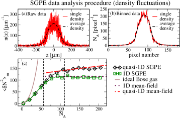
Figure 4: (Color online) Top row: quasi-1D SGPE density (noisy red curve) obtained from (a) a single numerical run (raw data), and (b) corresponding spatially binned data; dashed black curves display the density averaged over 1000 independent realisations. (c) $\langle\delta N^{2}\rangle_{m}$ endnote86 from the binned quasi-1D SGPE data (black diamonds) and 1D SGPE data (green squares), compared against correponding mean field results for an ideal Bose gas (brown solid line) 1D quasi-condensate (dotted maroon, horizontal) and quasi-1D quasi-condensate (dashed red); the thin, vertical dashed lines indicate the ‘crossover’ region where the interaction and thermal energies become comparable. This data is for $T=96$nK.

As we treat the atoms in the transverse modes in a static way, they give a non-zero contribution only to average properties, and so do not contribute to moments of the density fluctuations directly. However, as we found in Section III.1, atoms in these modes are well approximated as a degenerate ideal gas, for which $\langle\delta N^{2}\rangle_{\perp}\simeq\langle\delta N^{3}\rangle_{\perp}\simeq\langle N\rangle_{\perp}$ Armijo et al. (2010), and we therefore assume that these atoms contribute a factor $\langle N\rangle_{\perp}$ to both second and third moments. So, ultimately, we compute the total density fluctuations as $\langle\delta N^{p}\rangle=\langle\delta N^{p}\rangle_{z}+\langle N\rangle_{\perp}$, for $p=2,3$.

To illustrate our procedure, we plot in Fig.4 an example single run and average density profile both before (Fig.4(a)), and after (Fig.4(b)), spatial binning. Comparing these plots, it is clear that the binning procedure significantly smooths the raw single run data, as would be expected for this kind of a spatial coarse graining procedure; note that the binned data looks remarkably similar to the experimental fluctuating density profile shown in Armijo et al. (2010) (Fig. 1(c) of that work). We additionally show in Fig.4(c) the variance in the density fluctuations which results from the set of $1000$ fluctuating binned densities; this is plotted against the average number of atoms per pixel .

Making use of the thermodynamic relation $\langle\delta N^{2}\rangle=k_{B}T\Delta(\partial n/\partial\mu)_{T}$ Landau and Lifshitz (1980), it is possible to derive mean field results for the density fluctuations, based on both the ideal gas and quasi-condensate equations of state. The ideal gas result is Armijo et al. (2011)

$$\langle\delta N^{2}\rangle=\frac{1}{\lambda_{\mathrm{dB}}}\sum_{j=1}^{\infty}\frac{\sqrt{j}}{k_{B}T}\frac{e^{j\mu/k_{B}T}}{\sqrt{j}}\frac{1}{\left(1-e^{-j\hbar\omega_{\perp}/k_{B}T}\right)},$$ (6)

while using the 1D equation of state for a quasi-condensate ($\mu[n]=gn$) gives the simple result Estève et al. (2006) $\langle\delta N^{2}\rangle_{\rm 1D}={k_{B}T\Delta}/{g}$. Using instead the quasi-1D equation of state, Eq.(2), yields, $\langle\delta N^{2}\rangle_{\rm quasi-1D}=\langle\delta N^{2}\rangle_{\rm 1D}\left[1+{(\mu-V(z))}/{\hbar\omega_{\perp}}\right]$.

Within the higher density region of Fig.4(c), we show the mean field results due to the 1D and quasi-1D equations of state for a quasi-condensate. It is clear that the 1D SGPE shows good agreement with the 1D mean field result, whereas the quasi-1D SGPE instead agrees very well with the quasi-1D mean field prediction. The two vertical lines indicate the region where the interaction energy and the average thermal energy become comparable. For higher densities, interactions significantly reduce $\langle\delta N^{2}\rangle$ below the ideal gas prediction, and we see this is more pronounced in the 1D SGPE case relative to the quasi-1D SGPE data, as expected from the 1D and quasi-1D mean field predictions.

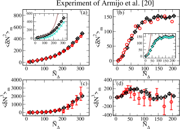
Figure 5: (Color online) Second (top row: (a)-(b)) and third (bottom row: (c)-(d)) moments of the atom number fluctuations from the quasi-1D SGPE data (black diamonds) and experimental data from the paper of Armijo et al.Armijo et al. (2010) (red circles). Temperatures are $T=376$nK (left images) and $T=96$nK (right images). Insets: axial (light blue crosses) versus axial plus transverse (black diamonds) contributions to the number fluctuations vs. the ideal gas result (brown solid line).

A key point from our analysis at this temperature, is that while the ideal gas equation of state is valid only for small densities, and the mean-field quasi-1D equation of state holds at high densities, the quasi-1D SGPE, like the experimental data, provides a smooth crossover between each of these regimes. This is because, in moving outwards from the centre of the trap in the presence of a quasi-condensate, at some point the gas changes phase to a thermal gas, and a mean field theory cannot be expected to accurately describe fluctuations in the transition region near the edge of the quasi-condensate.

Comparison to Experiment: Fig.5 shows a comparison of the experimental density fluctuation data obtained by Armijo et al. (red circles), and the quasi-1D SGPE model (black diamonds). We plot in the top row $\langle\delta N^{2}\rangle_{m}$, and in the bottom row $\langle\delta N^{3}\rangle_{m}$, each versus $\bar{N}_{\Delta}$ for two temperatures ($T=376$nK (left) and $96$nK (right)).

Concentrating on the $\langle\delta N^{2}\rangle_{m}$ data first, it is clear that the quasi-1D SGPE numerical results follow the experimental data well in both the high temperature (left) and low temperature cases (right images). Notice that as the high-density, quasi-condensate regime is reached in Fig.5(b), the 1D SGPE result (shown in Fig.4) would predict too great a reduction in density fluctuations relative to the experimental results, whereas the quasi-1D SGPE captures the experimental behaviour very well. Physically, this suggests that the effect of the transverse swelling of the quasi-condensate near the centre of the trap cannot be ignored for these parameters, and that the quasi-1D extension to the SGPE is therefore essential here.

Armijo et al. found a similar trend when comparing between their experimental data and the modified Yang-Yang model. While the Yang-Yang result matched the low density data well, at higher densities it displayed the same behaviour as the 1D SGPE result. Instead, Armijo et al. found the quasi-1D mean field result to better reproduce the experimental behaviour in the higher density quasi-condensate regime. So, as for the density profiles, we again find the 1D SGPE data to reproduce the 1D Yang-Yang behaviour, whereas the quasi-1D SGPE goes beyond the modified Yang-Yang model by capturing the quasi-1D behaviour found in the experiment in all regimes probed.

The results for the third moment (Fig.5, bottom row), $\langle\delta N^{3}\rangle_{m}$, also show good agreement between the quasi-1D SGPE and the experimental data (within the large experimental error bars).

The insets to Figs. 5(a)-(b) show clearly that the reduction in density fluctuations compared to the ideal gas prediction (brown solid line) is more pronounced in the low temperature case, where there is a higher quasi-condensate fraction. Contrary to this, the enhanced presence of thermal atoms in the high temperature case, provides an opportunity to test whether our approximate treatment of the transverse mode contribution to $\langle\delta N^{2}\rangle_{m}$, leads to the correct behaviour at low density. The results before (light blue crosses) and after (black diamonds) the transverse contribution is added are shown in the insets to Figs.5(a)-(b). This addition results in a noticeable shift upwards in the data of Fig.5(a) while for the lower temperature case, the difference following this addition is negligible. Comparing the SGPE data to the expected low density result, the ideal gas prediction for the same parameters (solid brown line), we see that adding a contribution $\langle N\rangle_{\perp}$ to the axial contribution fully captures the expected behaviour.

IV Conclusions

In conclusion, we have proposed and implemented a suitably modified one-dimensional stochastic Gross-Pitaevskii equation, which was shown to provide excellent ab initio predictions for both in situ experimental density profiles obtained by Trebbia et al.Trebbia et al. (2006) and van Amerongen et al.van Amerongen et al. (2008), and in situ density fluctuation data from the experiment of Armijo et al.Armijo et al. (2010). This was achieved by matching peak densities (equivalent to total atom number) to a hybrid scheme, which combines the aforementioned stochastic model with a previously reported approach based on treating transverse thermal modes as independent ideal Bose gases.

The study of density fluctuations showed that our combined approach captures all experimental regimes studied in a unified manner, smoothly interpolating between mean field models, whose individual validity is restricted to either the low density or high density regimes. Importantly, it was found that analyzing individual stochastic realizations in the same way as individual experimental runs, led to good agreement between the density statistics in each case.

Reducing our stochastic model to the previously tested one-dimensional stochastic Gross-Pitaevskii equation showed that: (i) the latter model is consistent with Yang-Yang predictions (in the weakly-interacting regime probed here), and that (ii) while both one-dimensional and quasi-one-dimensional approaches accurately reproduce equilibrium density profiles, they do so with slightly different chemical potentials.

The confidence gained from these successful comparisons suggests that the quasi-one-dimensional stochastic Gross-Pitaevskii model, which was proposed here as a hybrid of different previously implemented approaches, is an excellent model for describing quasi-condensate experiments at equilibrium; the extent to which this model can be directly applied to study dynamical features, such as experimentally-measured properties after expansion, remains to be investigated.

Acknowledgments.

We would like to thank Isabelle Bouchoule, and Aaldert van Amerongen and Klaasjan van Druten, for providing their experimental data for use in our comparison. NPP acknowledges discussions with Dimitri Frantzeskakis on the Gross-Pitaevskii equation in the quasi-one-dimensional regime, and Matt Davis, Geoff Lee and Karen Kheruntsyan for discussions on their related theoretical modeling. We also thank Carsten Henkel and Antonio Negretti for related discussions. This project was funded by the EPSRC.

References

- Bloch et al. (2008) I. Bloch, J. Dalibard, and W. Zwerger, Rev. Mod. Phys. 80, 885 (2008).
- Görlitz et al. (2001) A. Görlitz, J. M. Vogels, A. E. Leanhardt, C. Raman, T. L. Gustavson, J. R. Abo-Shaeer, A. P. Chikkatur, S. Gupta, S. Inouye, T. Rosenband, et al., Phys. Rev. Lett. 87, 130402 (2001).
- Rychtarik et al. (2004) D. Rychtarik, B. Engeser, H.-C. Nägerl, and R. Grimm, Phys. Rev. Lett. 92, 173003 (2004).
- Stock et al. (2005) S. Stock, Z. Hadzibabic, B. Battelier, M. Cheneau, and J. Dalibard, Phys. Rev. Lett. 95, 190403 (2005).
- Smith et al. (2005) N. L. Smith, W. H. Heathcote, G. Hechenblaikner, E. Nugent, and C. J. Foot, Journal of Physics B Atomic Molecular Physics 38, 223 (2005).
- Hadzibabic et al. (2006) Z. Hadzibabic, P. Krüger, M. Cheneau, B. Battelier, and J. Dalibard, Nature (London) 441, 1118 (2006).
- Schweikhard et al. (2007) V. Schweikhard, S. Tung, and E. A. Cornell, Phys. Rev. Lett. 99, 030401 (2007).
- Krüger et al. (2007) P. Krüger, Z. Hadzibabic, and J. Dalibard, Phys. Rev. Lett. 99, 040402 (2007).
- Hadzibabic et al. (2008) Z. Hadzibabic, P. Krüger, M. Cheneau, S. P. Rath, and J. Dalibard, New Journal of Physics 10, 045006 (2008), eprint 0712.1265.
- Cladé et al. (2009) P. Cladé, C. Ryu, A. Ramanathan, K. Helmerson, and W. D. Phillips, Phys. Rev. Lett. 102, 170401 (2009).
- Rath et al. (2010) S. P. Rath, T. Yefsah, K. J. Günter, M. Cheneau, R. Desbuquois, M. Holzmann, W. Krauth, and J. Dalibard, Phys. Rev. A 82, 013609 (2010).
- Tung et al. (2010) S. Tung, G. Lamporesi, D. Lobser, L. Xia, and E. A. Cornell, Phys. Rev. Lett. 105, 230408 (2010).
- Hung et al. (2011) C.-L. Hung, X. Zhang, N. Gemelke, and C. Chin, Nature (adv. online) (2011).
- Moritz et al. (2003) H. Moritz, T. Stöferle, M. Köhl, and T. Esslinger, Phys. Rev. Lett. 91, 250402 (2003).
- Paredes et al. (2004) B. Paredes, A. Widera, V. Murg, O. Mandel, S. Fölling, I. Cirac, G. V. Shlyapnikov, T. W. Hänsch, and I. Bloch, Nature (London) 429, 277 (2004).
- Kinoshita et al. (2004) T. Kinoshita, T. Wenger, and D. S. Weiss, Science 305, 1125 (2004).
- Cacciapuoti et al. (2003) L. Cacciapuoti, D. Hellweg, M. Kottke, T. Schulte, W. Ertmer, J. J. Arlt, K. Sengstock, L. Santos, and M. Lewenstein, Phys. Rev. A 68, 053612 (2003).
- Trebbia et al. (2006) J.-B. Trebbia, J. Esteve, C. I. Westbrook, and I. Bouchoule, Phys. Rev. Lett. 97, 250403 (2006).
- van Amerongen et al. (2008) A. H. van Amerongen, J. J. P. van Es, P. Wicke, K. V. Kheruntsyan, and N. J. van Druten, Phys. Rev. Lett. 100, 090402 (2008).
- Armijo et al. (2010) J. Armijo, T. Jacqmin, K. V. Kheruntsyan, and I. Bouchoule, Phys. Rev. Lett. 105, 230402 (2010).
- Armijo et al. (2011) J. Armijo, T. Jacqmin, K. Kheruntsyan, and I. Bouchoule, Phys. Rev. A 83, 021605 (2011).
- Estève et al. (2006) J. Estève, J.-B. Trebbia, T. Schumm, A. Aspect, C. I. Westbrook, and I. Bouchoule, Phys. Rev. Lett. 96, 130403 (2006).
- Dettmer et al. (2001) S. Dettmer, D. Hellweg, P. Ryytty, J. J. Arlt, W. Ertmer, K. Sengstock, D. S. Petrov, G. V. Shlyapnikov, H. Kreutzmann, L. Santos, et al., Phys. Rev. Lett. 87, 160406 (2001).
- Hellweg et al. (2003) D. Hellweg, L. Cacciapuoti, M. Kottke, T. Schulte, K. Sengstock, W. Ertmer, and J. J. Arlt, Phys. Rev. Lett. 91, 010406 (2003).
- Gerbier et al. (2003) F. Gerbier, J. H. Thywissen, S. Richard, M. Hugbart, P. Bouyer, and A. Aspect, Phys. Rev. A 67, 051602 (2003).
- Richard et al. (2003) S. Richard, F. Gerbier, J. H. Thywissen, M. Hugbart, P. Bouyer, and A. Aspect, Phys. Rev. Lett. 91, 010405 (2003).
- Manz et al. (2010) S. Manz, R. Bücker, T. Betz, C. Koller, S. Hofferberth, I. E. Mazets, A. Imambekov, E. Demler, A. Perrin, J. Schmiedmayer, et al., Phys. Rev. A 81, 031610 (2010).
- Gustavson et al. (1997) T. L. Gustavson, P. Bouyer, and M. A. Kasevich, Phys. Rev. Lett. 78, 2046 (1997).
- Hinds et al. (2001) E. A. Hinds, C. J. Vale, and M. G. Boshier, Phys. Rev. Lett. 86, 1462 (2001).
- Schumm et al. (2005) T. Schumm, S. Hofferberth, L. M. Andersson, S. Wildermuth, S. Groth, I. Bar-Joseph, J. Schmiedmayer, and P. Krüger, Nature Physics 1, 57 (2005).
- Hofferberth et al. (2006) S. Hofferberth, I. Lesanovsky, B. Fischer, J. Verdu, and J. Schmiedmayer, Nature Physics 2, 710 (2006).
- Fixler et al. (2007) J. B. Fixler, G. T. Foster, J. M. McGuirk, and M. A. Kasevich, Science 315, 74 (2007).
- Jo et al. (2007) G.-B. Jo, Y. Shin, S. Will, T. A. Pasquini, M. Saba, W. Ketterle, D. E. Pritchard, M. Vengalattore, and M. Prentiss, Phys. Rev. Lett. 98, 030407 (2007).
- Hofferberth et al. (2007) S. Hofferberth, I. Lesanovsky, B. Fischer, T. Schumm, and J. Schmiedmayer, Nature (London) 449, 324 (2007).
- Gross et al. (2010) C. Gross, T. Zibold, E. Nicklas, J. Estève, and M. K. Oberthaler, Nature (London) 464, 1165 (2010), eprint 1009.2374.
- Baumgärtner et al. (2010) F. Baumgärtner, R. J. Sewell, S. Eriksson, I. Llorente-Garcia, J. Dingjan, J. P. Cotter, and E. A. Hinds, Phys. Rev. Lett. 105, 243003 (2010).
- Hinds and Hughes (1999) E. A. Hinds and I. G. Hughes, Journal of Physics D Applied Physics 32, 119 (1999).
- Ott et al. (2001) H. Ott, J. Fortagh, G. Schlotterbeck, A. Grossmann, and C. Zimmermann, Phys. Rev. Lett. 87, 230401 (2001).
- Hänsel et al. (2001) W. Hänsel, P. Hommelhoff, T. W. Hänsch, and J. Reichel, Nature (London) 413, 498 (2001).
- Folman et al. (2002) R. Folman, P. Krüger, J. Schmiedmayer, J. Denschlag, and C. Henkel, Advances in Atomic and Molecular Physics 48, 263 (2002), eprint 0805.2613.
- Fortágh and Zimmermann (2007) J. Fortágh and C. Zimmermann, Rev. Mod. Phys. 79, 235 (2007).
- Reichel and Vuletic (2011) J. Reichel and V. E. Vuletic, Atom Chips (WILEY-VCH Verlag GmbH & Co. KGaA, Weinheim, 2011).
- Petrov et al. (2000) D. S. Petrov, G. V. Shlyapnikov, and J. T. M. Walraven, Phys. Rev. Lett. 85, 3745 (2000).
- Girardeau (1960) M. Girardeau, Journal of Mathematical Physics 1, 516 (1960).
- Al Khawaja et al. (2003) U. Al Khawaja, N. P. Proukakis, J. O. Andersen, M. W. J. Romans, and H. T. C. Stoof, Phys. Rev. A 68, 043603 (2003).
- Popov (1983) V. N. Popov, Functional Integrals in Quantum Field Theory and Statistical Physics (Reidel, Dordrecht, 1983), chap. 6.
- Stoof (1999) H. T. C. Stoof, J. Low Temp. Phys. 114, 11 (1999).
- Stoof and Bijlsma (2001) H. T. C. Stoof and M. J. Bijlsma, J. Low Temp. Phys. 124, 431 (2001).
- Gardiner and Davis (2003) C. W. Gardiner and M. J. Davis, J. Phys. B 36, 4731 (2003).
- Stringari (1998) S. Stringari, Phys. Rev. A 58, 2385 (1998).
- Petrov et al. (2001) D. S. Petrov, G. V. Shlyapnikov, and J. T. M. Walraven, Phys. Rev. Lett. 87, 050404 (2001).
- Svistunov (1991) B. Svistunov, J. Moscow Phys. Soc. 1, 373 (1991).
- Duine and Stoof (2001) R. A. Duine and H. T. C. Stoof, Phys. Rev. A 65, 013603 (2001).
- Davis et al. (2001) M. J. Davis, S. A. Morgan, and K. Burnett, Phys. Rev. Lett. 87, 160402 (2001).
- Sinatra et al. (2001) A. Sinatra, C. Lobo, and Y. Castin, Phys. Rev. Lett. 87, 210404 (2001).
- Goral et al. (2001) K. Goral, M. Gajda, and K. M. Rzazewski, Optics Express 8, 92 (2001).
- Penckwitt et al. (2002) A. A. Penckwitt, R. J. Ballagh, and C. W. Gardiner, Phys. Rev. Lett. 89, 260402 (2002).
- Duine et al. (2004) R. A. Duine, B. W. A. Leurs, and H. T. C. Stoof, Phys. Rev. A 69, 053623 (2004).
- Krüger et al. (2010) P. Krüger, S. Hofferberth, I. E. Mazets, I. Lesanovsky, and J. Schmiedmayer, Phys. Rev. Lett. 105, 265302 (2010).
- Fuchs et al. (2003) J. N. Fuchs, X. Leyronas, and R. Combescot, Phys. Rev. A 68, 043610 (2003).
- Gerbier (2004) F. Gerbier, Europhys. Lett. 66, 771 (2004).
- Muñoz Mateo and Delgado (2007) A. Muñoz Mateo and V. Delgado, Phys. Rev. A 75, 063610 (2007).
- Frantzeskakis (2010) D. J. Frantzeskakis, Journal of Physics A Mathematical General 43, 213001 (2010).
- Menotti and Stringari (2002) C. Menotti and S. Stringari, Phys. Rev. A 66, 043610 (2002).
- Proukakis and Jackson (2008) N. P. Proukakis and B. Jackson, J. Phys. B 41, 203002 (2008).
- Cockburn et al. (2010) S. P. Cockburn, A. Negretti, N. P. Proukakis, and C. Henkel, (accepted in Phys. Rev. A) (2010), eprint arXiv:1012.1512.
- Wright et al. (2010) T. M. Wright, N. P. Proukakis, and M. J. Davis (2010), eprint arXiv:1011.6289.
- Naraschewski and Glauber (1999) M. Naraschewski and R. J. Glauber, Phys. Rev. A 59, 4595 (1999).
- Prokof’ev and Svistunov (2002) N. Prokof’ev and B. Svistunov, Phys. Rev. A 66, 043608 (2002).
- Proukakis (2006) N. P. Proukakis, Phys. Rev. A 74, 053617 (2006).
- Bisset and Blakie (2009) R. N. Bisset and P. B. Blakie, Phys. Rev. A 80, 035602 (2009).
- Yang and Yang (1969) C. N. Yang and C. P. Yang, Journal of Mathematical Physics 10, 1115 (1969).
- Kheruntsyan et al. (2010) K. Kheruntsyan, M. J. Davis, P. B. Blakie, A. H. van Amerongen, and N. J. van Druten, Poster at ICAP (2010).
- Blakie et al. (2008) P. B. Blakie, A. S. Bradley, M. J. Davis, R. J. Ballagh, and C. W. Gardiner, Adv. Phys. 57, 363 (2008).
- Shvarchuck et al. (2002) I. Shvarchuck, C. Buggle, D. S. Petrov, K. Dieckmann, M. Zielonkowski, M. Kemmann, T. G. Tiecke, W. von Klitzing, G. V. Shlyapnikov, and J. T. M. Walraven, Phys. Rev. Lett. 89, 270404 (2002).
- Landau and Lifshitz (1980) L. D. Landau and E. M. Lifshitz, Statistical Physics, Part 1., vol. Vol. 5 (3rd ed.) (Butterworth-Heinemann, 1980).
- Cockburn et al. (2010) S. P. Cockburn, H. E. Nistazakis, T. P. Horikis, P. G. Kevrekidis, N. P. Proukakis, and D. J. Frantzeskakis, Phys. Rev. Lett. 104, 174101 (2010).
- Weiler et al. (2008) C. N. Weiler, T. W. Neely, D. R. Scherer, A. S. Bradley, M. J. Davis, and B. P. Anderson, Nature 455, 948 (2008), eprint 0807.3323.
- Damski and Zurek (2010) B. Damski and W. H. Zurek, Phys. Rev. Lett. 104, 160404 (2010).
- Das et al. (2011) A. Das, J. Sabbatini, and W. H. Zurek (2011), eprint arXiv:1102.5474.
- Cockburn and Proukakis (2009) S. P. Cockburn and N. P. Proukakis, Las. Phys. 19, 558 (2009).
- Zaremba et al. (1999) E. Zaremba, T. Nikuni, and A. Griffin, J. Low Temp. Phys. 116, 277 (1999).
- Andersen et al. (2002) J. Andersen, U. Al Khawaja, and H. Stoof, Phys. Rev. Lett. 88, 070407 (2002).
- Al Khawaja et al. (2002) U. Al Khawaja, J. O. Andersen, N. P. Proukakis, and H. T. C. Stoof, Phys. Rev. A 66, 013615 (2002), erratum: Phys. Rev. A 66, 059902(E) (2002).