Stability of the Zagreb realization of the Carnegie-Mellon-Berkeley coupled-channels unitary model

Abstract

In ref. Mirza2011 we have used the Zagreb realization of Carnegie-Melon-Berkeley coupled-channel, unitary model as a tool for extracting pole positions from the world collection of partial wave data, with the aim of eliminating model dependence in pole-search procedures. In order that the method is sensible, we in this paper discuss the stability of the method with respect to the strong variation of different model ingredients. We show that the Zagreb CMB procedure is very stable with strong variation of the model assumptions, and that it can reliably predict the pole positions of the fitted partial wave amplitudes.

I Introduction

Various analyses of meson-baryon scattering designed with the goal to extract resonance properties from data are available in literature. They fundamentally differ in technical approach how the model is implemented (effective Lagrangian approach, K matrix formalism, K matrix approximation, phenomenological coupled-channel formalism, t-channel dispersion relations, hyperbolic dispersion relations, e.t.c.), however most of them strongly insist in obeying fundamental physics principles like Lorentz invariance, crossing symmetry, unitarity and analyticity. In ref. Mirza2011 , we have extracted the pole positions from a “world collection” of partial wave data and partial-wave amplitudes understanding them as partial-wave data, with the aim of eliminating the model dependence from the individual pole-search procedures. We have analyzed some major PWA amplitudes like: i) Karlsruhe-Helsinki (KH80) amplitudes KH80 for the $\pi$N elastic scattering, where fixed t-channel dispersion relations are combined with Pietarinen expansion to impose and maintain point-to-point analyticity; ii) VPI/GWU single energy (GWU-SES) GWUWEB , and energy dependent solutions (WI08) Arn04 ; GWUWEB where Chew-Mandelstam K-matrix formalism together with dispersion relation constraints is applied; iii) dynamic coupled-channel Lagrangian approaches from EBAC model Diaz07 ; Dur08 which is based on an energy independent Hamiltonian which is derived from a set of Lagrangians by using a unitary transformation method Matsuyama2007 ; iv) Jülich model Juelich which is also a dynamical coupled-channels model of meson production reactions in the nucleon resonance region which includes $\pi$N, $\eta$N, $\pi\Delta$, $\sigma$N, and $\rho$N channels; v) Dubna-Mainz-Taipei (DMT) model Che03 ; Che07 , a meson-exchange model for pion-nucleon scattering which was constructed using a three-dimensional reduction scheme of the Bethe-Salpeter equation for a model Lagrangian involving $\pi$, $\eta$, N, $\Delta$, $\rho$, and $\sigma$ fields; and vi) and the Giessen K-matrix approximation (analyticity violating) model Giessen . Let us not fail to mention other, important theoretical approaches like Cutkosky CMU-LBL phenomenological coupled channel model Cut79 , Pittsburgh phenomenological coupled-channel model Vrana2000 and Bonn-Gatchina K-matrix approach without dispersive part BonnGatchina , which are for different reasons not included in analysis of ref. Mirza2011 .

In this paper we discuss how stable our recommended procedure is with respect to our model assumptions in order to give an quantitative estimate how confident the results of that report actually are.

We have been triggered to start the whole enterprise by the present uncertainty how to make the least model dependent comparison between scattering theories which analyze experimental data on one side, and QCD models or lattice QCD calculations on the other. In other words, we have been dealing with the problem how to precisely define what a resonance actually is. And it has to be done on both sides, on scattering theory side, as well as on the QCD side.

One, and the most intuitive way to define a resonance in a scattering process, is to define it as an intermediate state of two particles when they, because of attractive interaction, dwell in the vicinity of each other longer then in a standard scattering process. When this definition is transformed into the language of scattering theory, since 1976 it seems that, as Höhler has said in Hoe2001 : “It is ‘noncontroversial among theorists’ (see Chew Chew1976 and the references in my ‘pole-emics’, p.697 in ref. Hoe2000 ) that in S-matrix theory the effects of resonances follow from first order poles in the 2nd sheet.” However, if resonances are to be identified with the first order poles in the 2nd sheet, we can not but observe that characterizing such states, namely identifying and quantifying scattering matrix poles in the complex energy plane turns out to be quite a challenge.

Different methods aimed onto identifying one of the possible repercussions of a resonant state onto measurable quantities have been developed. First it has been speculated that a Breit-Wigner function should be a good representation of the complex energy pole, so the Breit-Wigner formula for spin zero particles together with its generalization to the non-zero spin case has been developed in 1936 (see an illustrative discussion in Cottingham and Greenwood, p.241 in ref. Breit-Wigner ). Then in DalitzMoorhouse Dalitz and Moorehouse considered the scattering matrix eigenphases, and their rapid increase through $\pi$/2 have been taken as a signature of pinpointing a scattering matrix pole (namely, the corresponding eigenvalue of the reaction matrix K = i (S-1)/(S+1) then has a pole at this energy Dalitz61 ). Finally, closely related to the afore two, the quick backwards looping of Argand diagram have been also extensively discussed by Dalitz and Moorehouse DalitzMoorhouse .

As the time passed by, the real meaning of these methods, namely the fact that they are devised only to reach the scattering matrix pole in the complex energy plane in a certain approximation, tended to be overlooked. These methods alone have been identified as resonance definition procedures, and what they found has been proclaimed to be a resonant state. However, their inherent model dependence, like for instance unitary addition of non-resonant background, has been systematically neglected (see the elaboration on Breit-Wigner model dependence in ref. Hoe2000 ). The problems of eigenphases, linked to the manifest violation of Neumann-Wigner no-crossing theorem Neumann-Wigner29 when rapidly going through $\pi/2$ even for the case of simply constant background terms, have been suppressed in spite of the extensive elaboration of the problem given by Dalitz and Moorhouse in ref. DalitzMoorhouse . They have explicitly said that: “With such a complexity of branch cuts without physical significance, we must conclude that the eigenphase representation for the S matrix is not generally a useful representation for the scattering in the neighbourhood of a resonance”, but have anyhow allowed the possibility to use it in a more restricted situation: “However, we should emphasize also that the eigenphase representation is a perfectly acceptable and economical representation of the S matrix in situations where the eigenphases vary slowly and do not cross”. The single-channel nature of pole search methods (with the exception of the time delay which is in principle of multi-channel character) also did not represent much of a problem,because experimental data in inelastic channels were scarce. The fact that a single-channel procedure can not reveal much information about resonant states being ‘far away’ from that channel, has also been suppressed.

In ref. Mirza2011 we have returned to the root of the problem – we have fully respected that we are looking for the pole in the complex energy plane having at our disposal only data on the real axes, and instead of using different pole-extraction methods to extract a pole per resonance, we have suggested to use only one, Zagreb CMB method Bat98 ; Batinic2010 and extract poles from a selected collection of partial wave amplitudes simultaneously. We have decided to use only one method to extract pole positions from all published partial waves analyses, and inspect the result with the aim to distinguish which part of the disagreement in pole positions is coming from the different analytic structure, and which is coming from the different input (different PWA functions). In other words, we have taken all sets of partial-wave amplitudes, treated them as nothing else but a good, energy dependent representations of all analyzed experimental data, and extracted the poles which are needed by the CMB method. We observe that even when practically all analyzed PWA use very similar input data set, their PWA solutions do differ in spite of reporting the similar quality of fit to the input data (similar reduced $\chi^{2}$). So, from the theoretical point of view, they equally well describe the experiment. And now these, however similar, but still different curves through different analytic continuations of each model generate corresponding and different sets of poles. So, in addition to the issue of slightly different input, the error of unknown analyticity is superimposed to it. It is important to realize that these poles, even for the identical set of input amplitudes, should not necessarily coincide, because the models used for analytic continuation are intrinsically different in their analytic form (for illustration see ref. Ceci2011 ). The idea of using only one model (Zagreb CMB) to extract the set of poles from different PWA treating them as partial wave data boils down to testing the internal agreement of input data sets. In this way, the difference between poles of various solutions is attributed only to the under-determinacy of input data and not to the analytic structure of the models in question. Simply, different poles obtained in this way quantify the difference in PWA solutions with respect to the similar input, and disregard the different analytic form used to obtain them. In this manner, all uncertainties originating from different analytic properties of different models are avoided, and the only remaining errors are the quality of the input and the precision of CMB method itself. Therefore, averaging and error analysis of pole positions is sensible, and can be safely carried out. To answer the question of a correct choice of analytic form is a more complex problem and will be addressed elsewhere.

In this paper we discuss how sensitive this method is to CMB model assumptions when our input data set is well defined. We have first chosen the reliable input data set, a data set for which the minimization is fast, stable and unambiguous. Then we have identified our model assumptions, specific ones which we may check, and more general ones which are unfortunately beyond our reach. The general ones, like the isobar character of the model representing the unstable channels with a quasi two body channel with decay properly taken into account, could not be checked directly. Other ones, like for instance the form of the channel propagator (channel-resonance vertex function), dependence on the dispersion integral subtraction constant, background parameterization, number of channels, mass of the effective channel, etc. we check directly. Instead of taking different recipes for each model assumption, we have simply modified the used functional form with an completely arbitrary function which is just changing the range of interest, and repeated the fit. In this way the stability with respect to different model assumption is performed.

II General idea

If we want to apply a CMB formalism with the intention of extracting pole parameters from a “world collection” of partial wave data and partial wave amplitudes, one has to answer a natural question how stable the formalism itself is with respect to model assumptions. We are aware that we can test the sensitivity of the model upon its ingredients, but the reliability of the isobar model itself can not be tested in this way. Therefore, at this instant, we still can not say how strongly our answer depends on the fact that we assume that the interaction mechanism of isobar intermediate states is the only relevant one.

Our present analysis involves yet another approximation, and that is that possible three body states are effectively represented by a group of two body ones. We shall not test this hypothesis either, even knowing that according to some considerations these effects can build up to 30%.

Even before starting the procedure, we have to answer a nontrivial question:
“What is the optimal input data base so that our pole positions are unique for the model without any modifications?”

Once this answer is given, we have to analyze how the final pole positions depend on model assumptions like (i) shape of the channel-resonance form factor; (ii) choice of the dispersion integral subtraction constant; (iii) masses of the effective channel; (iv) number of channels; (v) type of the background parameterization.
The driving idea of this paper is:
“To drastically modify only one part of the model at a time, and then make a fit to the chosen data base. The dissipation of pole positions known from the original fit will give us information how important certain part of the model is for the stability of the solution.”

We will just add that these changes are intentionally artificial, aimed only at obtaining the effect, and not paying attention to the physical meaning.

III Formalism

The CMB model is isobar, coupled-channel, analytic, and unitary model, where the T matrix in a given channel is assumed to be a sum over the contributions from a number of intermediate particles (resonance and background contributions). The coupling of the channel asymptotic states to these intermediate particles determines the imaginary part of the channel function, and is represented effectively with a separable function. The real part of the channel function is calculated by the dispersion relation technique, thus ensuring analyticity. Besides the known resonance contributions, the background contributions are included via additional terms with poles below the $\pi$N threshold. Due to the clear analytic and separable structure of the model, finding the pole positions in CMB model is trimmed down to the generalization of the dispersion integral for the channel propagator from real axes to the full complex energy plane, and this is a very well defined procedure. In practice, we instead use a very stable, and numerically much faster analytic continuation method based on the Pietarienen expansion Pietarinen in order to extrapolate the real valued channel propagator into the complex energy plane.

III.1 Formulae

Our current partial-wave analysis Bat98 is based on the manifestly unitary, multichannel CMB approach of ref. Cut79 . The most prominent property of this approach is analyticity of partial waves with respect to Mandelstam $s$ variable. In every discussion of partial-wave poles, analyticity plays a crucial role since the poles are situated in a complex plane, away from physical region, and our measuring abilities are restricted to the real energy axis only. To gain any knowledge about the nature of partial-wave singularities would be impossible if partial waves were not analytic. Therefore, the ability to calculate pole positions is not just a benefit of the CMB model’s analyticity but also a necessity for resonance extraction. In this approach, the resonance itself is considered to exist if there is an associated partial-wave pole in the “unphysical” sheet.

We use the multichannel $T$ matrix related to the scattering matrix $S$ as:

$$S_{ab}(s)=\delta_{ab}+2\,i\,T_{ab}(s),$$

where $\delta_{ab}$ is Kronecker delta symbol. The T-matrix matrix element is in the CMB model given as:

$$T_{ab}^{JL}(s)=\sum_{i,j=1}^{N^{JL}}f_{a}^{JL}(s)\sqrt{\rho_{a}(s)}\gamma_{ai}^{JL}G_{ij}^{JL}(s)\gamma_{jb}^{JL}\sqrt{\rho_{b}(s)}f_{b}^{JL}(s)$$ (1)

where $a(b)$ represents the outgoing (incoming) channel. In our analyses we use $a,b=\pi N,\eta N,\pi^{2}N$. The initial and final channel $b(a)$ couple through intermediate particles labeled $i$ and $j$. The factors $\gamma_{ia}$ are energy-independent parameters occurring graphically at the vertex between channel $a$ and intermediate particle $i$ and are determined by fitting procedure. Also occurring at each initial or final vertex is form factor $f_{a}^{JL}(s)$

$$f_{a}^{JL}(s)=\left(\frac{q_{a}}{Q_{1a}+\sqrt{Q_{2a}^{2}+q_{a}^{2}}}\right)^{L},$$ (2)

and phase-space factor $\rho_{a}(s)$

$$\rho_{a}(s)=\frac{q_{a}(s)}{\sqrt{s}},$$ (3)

where $s=W^{2}$ is a Mandelstam variable, and $q_{a}(s)$ is the meson momentum for any of the three channels given as

$$q_{a}(s)=\frac{\sqrt{(s-(m+m_{a})^{2})(s-(m-m_{a})^{2})}}{2\sqrt{s}}.$$ (4)

Furthermore, $L$ is the angular momentum in channel $a$, and $Q_{1a}$, $Q_{2a}$ are constants. The factor $f_{a}^{JL}(s)$ provides appropriate threshold behavior on the right-hand cut, and also produces a left-hand branch cut in the $s$ plane. Parameters $Q_{1a}$ and $Q_{2a}$ are chosen to determine the branch point and strength of the left-hand branch cut. In our analyses they have been taken to be the same, and are fixed to the mass of the channel meson $a$.

$G_{ij}^{JL}$ is a dressed propagator for partial wave $JL$ and particles $i$ and $j$, and may be written in terms of a diagonal bare propagator $G_{ij}^{0JL}$ and a self-energy matrix $\Sigma_{kl}^{JL}$ using Dyson equation

$$G_{ij}^{JL}(s) = G_{ij}^{0JL}(s)+\sum_{k,l=1}^{N^{JL}}G_{ik}^{0JL}(s)\Sigma_{kl}^{JL}(s)G_{ij}^{JL}(s).$$ (5)

The bare propagator

$$G_{ij}^{0JL}(s)=\frac{e_{i}\delta_{ij}}{s_{i}-s}$$ (6)

has a pole at the real value $s_{i}$. The sign $e_{i}=\pm 1$ must be chosen to be positive for poles above the elastic threshold which correspond to resonance.

The nonresonant background is described by a meromorphic function, in most of the cases consisting of two terms of the form (6) with pole positions below $\pi N$ threshold. For that case, the signs of the terms are opposite. The positive sign correspond to the repulsive and the negative sign to the attractive potential. In principle the number of poles can be increased arbitrarily (see the next subsection on background representation), but in reality the number is never larger than three.

$\Sigma_{kl}^{JL}$ is the self-energy term for the particle propagator

$$\Sigma_{kl}^{JL}(s)=\sum_{a}\gamma_{ka}^{JL}\cdot\Phi_{a}^{JL}(s)\cdot\gamma_{la}^{JL}$$ (7)

The $\Phi_{a}^{JL}(s)$ are called “channel propagators”. They are constructed in an approximation that treats each channel as containing only two particles. We require that $T_{ab}^{JL}$ have, in all channels, correct unitarity and analyticity properties consistent with a quasi-two-body approximation.

The imaginary part of $\Phi_{a}^{JL}(s)$ is the effective phase-space factor for channel $a$:

$$\mathrm{Im}\ \Phi_{a}^{JL}(s)=[f_{a}^{JL}(s)]^{2}\rho_{a}(s).$$ (8)

The channel propagator is evaluated on the real axes only

$$\mathrm{Im}\,\Phi(x)=\frac{\left[q(x)\right]^{2L+1}}{\sqrt{x}\,\left\{Q_{1}+\sqrt{Q_{2}^{2}+\left[q(x)\right]^{2}}\right\}^{2L}},\vspace*{0.1cm}$$ (9)

where by $x$ we stress the fact that values are on the real axes. The real part of $\Phi_{a}^{JL}(x)$ is calculated using a subtracted dispersion relation

$$\mathrm{Re}\,\Phi(x)={\mathrm{Re}\,\Phi(x_{0})}+\frac{x-x_{0}}{\pi}\,\,\mathrm{P}\int_{x_{a}}^{\infty}\frac{\mathrm{Im}\,\Phi(x^{\prime})\,dx^{\prime}}{(x^{\prime}-x)(x^{\prime}-x_{0})}.$$ (10)

where $x_{a}=(m+m_{a})^{2}$ and $\mathrm{Re}\,\Phi(x_{0})$ is a subtraction constant at the subtraction point $x_{0}$. In all publications Bat98 ; Batinic2010 we have chosen the convention that $x_{0}=x_{a}$ and $\mathrm{Re}\,\Phi(x_{0})$ = 0, but this is not necessarily so. For better understanding, the structure of the channel-intermediate particle form factor and its relation to the full T-matrix is given in Fig. 1.

Figure 1: (Color online) Parameterization of channel-intermediate particle vertex in CMB model.

We give a matrix form of the final T-matrix as defined in Eq. (1):

$$\hat{T}(s)=\sqrt{\mathrm{Im}\hat{\Phi}(s)}\cdot\hat{\gamma}^{\rm T}\cdot\frac{\hat{G}_{0}(s)}{I-\left[\hat{\gamma}\cdot\hat{\Phi}(s)\cdot\hat{\gamma}{\rm{}^{T}}\right]\cdot\hat{G}_{0}(s)}\cdot\hat{\gamma}\cdot\sqrt{\mathrm{Im}\hat{\Phi}(s)}$$ (11)

III.2 Background contributions

Theoretically, background term is in principle a free function of energy. However, an approximation is very often used that one may decompose the background term into a finite number of unphysical pole terms, i.e., the background is a meromorphic function. This approach is very convenient for the CMB type calculation because integral equations for the background poles are solved in the identical manner as for physical ones, so has it been applied and strongly defended by Cutkosky et al Cut79 in CMB PWA. Zagreb group has taken it over in Bat98 .

Let us elaborate on what we have actually done when we assumed that the background indeed is a meromorphic function. In that case, instead of solving a nonlinear equation for the T-matrix pole positions when the background has a general energy dependent form, we have actually introduced a new type of poles which mimic the background. Here we rely on the approximation that the solutions of a nonlinear equation with general type background will be close to the solutions of “pole-type” equation, the equation when the meromorphic background is very close to the original function. Consequently, we do not have one, but two types of T-matrix poles: i) poles which correspond to the physical internal singularities; and ii) poles which correspond to the background. We call the first type genuine poles, and the second ones we call dynamic poles.

The speculative question is: “How realistic the meromorphic background approximation actually is?”

III.3 Pole extraction procedure

The poles of the T matrix given in Eq. (1) are found by solving the equation:

$$\mathrm{det}\,\,G^{-1}(s)=\mathrm{det}\,\left[e_{ij}\delta_{ij}(s_{i}-s)-\Sigma_{ij}\right]=0.$$ (12)

This ia a complex equation, and can be solved only by analytic continuation of the physical, experimentally accessible T-matrix values which of course lie on the real energy axes into the complex energy plane. Let us observe that the only part of the Eq. (12) which is not defined in the complex energy plane is the channel propagator which is defined on the real axes only.

Therefore, the problem of finding the poles of Eq. (1) is reduced to analytic continuation of the channel propagator.

This analytic continuation can be done either by numeric principle value integration, or by Pietarinen expansion. The numeric integration of the channel propagator, used in ref. Bat98 , is a straightforward procedure, but requires a lot of computer time. Instead, we have used a more elegant way, a Pietarinen expansion used by Karlsruhe-Helsinki group KH80 .
From Eq. (9) it is evident that $\Phi(s)$ has a square-root type singularity in cm momentum, and analytic continuation into the complex energy plane should take it into account. Instead of calculating the dispersion integral (10) for each point in complex plane, we decided to expend the function $\Phi(s)$ in power series of a new variable, which accounts for all analyticity requirements. We use the expansion (similar to Pietarinen’s in Ref. Pietarinen or Ciuli’s Ciu62 )

$$\Phi_{\mathrm{I}}(s)=\sum_{n=0}^{N}C_{n}\,\left[Z_{\mathrm{I}}(s)\right]^{n},$$ (13)

where $C_{n}$ are coefficients of expansion. The new channel dependent variable is given by its principal branch

$$Z_{\mathrm{I}}(s)=\frac{\alpha-\sqrt{x_{a}-s}}{\alpha+\sqrt{x_{a}-s}},$$ (14)

with the tuning parameter $\alpha$. This function is fitted to a data set consisting of imaginary parts of $\Phi(x)$ from Eq. (9) and real parts of $\Phi(x)$ calculated from dispersion relation (10), both of them evaluated at real axis (hence $x$).

The general idea is that the $\Phi(s)$ inherits analytic structure from $Z(s)$. We obtained parameters $\alpha$ and coefficients $C_{n}$ for each channel, and for all analyzed partial waves. The least-square fit is considered to be good if it meets following conditions: (i) small number of coefficients $C_{n}$ needed (7 or 8, at most), (ii) the function fitted to the part of data set, when extrapolated outside of the fitted region is consistent with the rest of data, and (iii) fitting just imaginary part of $\Phi(x)$ produces real part that is in agreement with values obtained from (10).

The channel propagator given by expansion (13) is obtained quite accurately on the real axes, and as the expansion possess a correct analytic structure of 2$\rightarrow$2 scattering processes, the deviation between expansion (13) and the correct value given by Eq. (10) should be fairly small for the resonant region in the vicinity of physical axis.

Every channel opening is responsible for two Riemann sheets: the first (physical) sheet with physical partial waves, and the secondary (unphysical) sheet with resonant poles. To get to the unphysical sheet it is enough to use the second branch of $Z(z)$

$$Z_{\mathrm{II}}(s)=\frac{\alpha+\sqrt{x_{a}-s}}{\alpha-\sqrt{x_{a}-s}}.$$ (15)

Finally, it is evident from Eq. (1) that all poles of each partial wave must by construction be the same in all channels and, in fact, equal to the poles of the resolvent $\mathbf{G}(s)$.

In practice, for the S-wave $\pi$N channel propagator, the realization of the Pietarinen expansion on the real axes is shown in Fig. 2. Red points represent the imaginary part of the channel propagator $\Phi$ on the real axes, and are given by Eq. (9), blue points represent the real part of the channel propagator $\Phi$ on the real axes, and are calculated by the dispersion relation (10), and the full line represent the function $\Phi_{\mathrm{I}}$(x), a complex function defined on the full complex energy plane, and having a proper branch points and corresponding cuts for each channel.

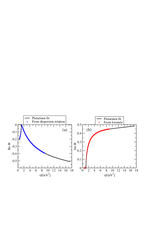
Figure 2: (Color online) Pietarinen expansion for the S₁₁ partial wave.

As the channel propagator is now known in the whole complex energy plane, the equation Eq. (12) was solved numerically as the complex function of the complex arguments. In reality, instead of looking for zeroes of Eq. (12) we have looked for the poles of $\mathrm{det}\,G(s)^{-1}$. In practice we have calculated $|\mathrm{det}\,G|$ as a function of Re(s) and Im(s) - (3D plot) specifying exactly the Riemann sheet in question (we have defined the appropriate momentum square roots in the channel propagator). Then we have looked for the values of Real(s) and Imag(s) when $|\mathrm{det}\,G|$ becomes bigger then an arbitrary number.

We regarded the obtained values of Re(s₀) and Im(s₀) as pole positions, and illustrate the procedure in Fig. 3.

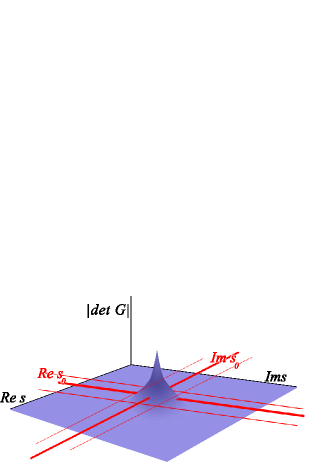
Figure 3: (Color online) The principle of numerical finding the pole positions using Eq. (12) with the Pietarinen expansion of the channel propagator.

IV Sources of model dependence

Understanding that the general assumptions of the model like its isobar, two body character in which the three and more body channels are identified with a quasi two body channels are properly taken into account, we now identify other sources of model dependence which at the present moment represent additional, systematic and uncontrollable uncertainties:

1. the form of the channel propagator (meson-resonance vertex function)

   • its asymptotic part

   • its intermediate part

   • threshold behavior

2. dispersion integral subtraction constant

3. background parameterization

4. number of channels

5. mass of the effective channel

The idea of present work is to allow for the extensive change of the chosen model features, and see at which level the pole positions are starting to move. The extensive change of the chosen model feature is realized by multiplying it with a freely chosen function (no physical meaning whatsoever) which influences only the tested part of the model assumption, and parameters are varied in such a way that the change in the analyzed part in/decreases from $\sim$ 10% to more than 100% of the original value.

Prerequisite of such a procedure is that the input data base is such that it ensures a confident and reliable fit. Namely, we have to be positive that the variation of the extracting pole positions is coming from changing the ingredients of the model drastically, and that the fit to the input data base converges fast and uniquely. Therefore, we first describe the choice of the input data base, and then we test the ingredients of the model.

V Testing the model dependence

V.1 Defining the input data set

If we want to test the stability of the model with respect to its ingredients, we first have to choose such an input data base (set of input data our modified model will fit) for which the fitting procedure with original model is fast, unique and reproducible. In other words, we want to choose such an input data base for which the original model reproduces its own, input values safely, quickly and unambiguously. In that case, we can vary the ingredients of the model, and claim that the resulting shift in pole positions is the result of change in the model itself, and not the consequence of inadequate input data. This is in a way a test of internal consistency of the model, the proof that the model when fitting its own result obtains the parameters that were used to generate the input (logistic tautology). However, when we start changing the ingredients of the model, the analytic structure of the model itself is changed, so we necessarily expect to obtain a different set of resulting pole parameters. The deviations of these parameters from the original input values are now the measure of sensitivity of the model to different model assumptions.

As the input for this work we have chosen partial wave amplitudes of Zagreb model Bat98 . Once the input parameters are chosen and fixed (bare poles and channel-resonance coupling constants $\gamma$), we have all partial waves at our disposal. In this section we test how stable the fit is for the first three lowest angular momentum partial waves S₁₁, P₁₁ and D₁₃ with respect to how many channel data sets we have used.

In Zagreb model we have three set of partial wave amplitudes at our disposal: $\pi\!N\!\rightarrow\!\pi\!N$, $\pi\!N\!\rightarrow\!\eta N\>$and $\pi\!N\!\rightarrow\!\pi^{2}N$. In principle, all Zagreb PWA are smooth energy dependent functions. We could have fitted these solutions directly. However, we have been of an opinion that by doing so it would introduce too many analytic constraints coming from the fact that these solutions “memorize” the analytic form of CMB formalism used to obtain them. We wanted to eliminate these additional constraints, so we have distributed the energy continuous Zagreb solutions by the recipe given in ref. Ceci06 .

Instead of using smooth theoretical curves and avoid pathologically small $\chi_{R}^{2}$ , we constructed pseudo data points by normally distributing the model input in order to simulate the statistical nature of really measured data. The standard deviation $\sigma$ was set to 0.02, similar to the average error value of GWU data Arn04 ; GWUWEB . By using this procedure we were able to produce a set of $\pi\!N\!\rightarrow\!\pi\!N$, $\pi\!N\!\rightarrow\!\eta N\>$and $\pi\!N\!\rightarrow\!\pi^{2}N\>$ partial-wave data which reproduced the experiment, and when fitted, they gave realistic $\chi^{2}$ values comparable with those obtained by GWU/VPI SES fits. The pole parameters of the input data set are given in Table 1. The input data sets together with our fit are shown in Fig. 4.

To simplify the discussion, we introduce the generic abbreviation L${}_{2I2J}($mass$)$ for each pole position produced in Zagreb model.

To illustrate, the S₁₁ (1518) pole denotes the first, 1518 MeV S₁₁ pole, and is identified with the N(1535) S₁₁ PDG resonance. Observe that all Zagreb solutions correspond to an existing PDG resonant state, with the exception of two P₁₁ intermediate energy solutions. In Zagreb model we get two P₁₁ solutions: P₁₁ (1708) pole which is in Bat98 ; Batinic2010 identified with N(1710) P₁₁ state, and a new solution P₁₁ (1728) which is not confirmed by PDG.

In Tables 2, 3, 4 we show the results of the test in which we have looked for the optimal number of fitted channels required for the stable fit. Results obtained by fitting only elastic channel are denoted by Fit 1. Fit 2 stands for a case when the $\pi N\rightarrow\eta N$ channel is included in a fit in addition to elastic channel. Results denoted by Standard fit are obtained by fitting all three channel simultaneously. The reduced chi-squared for the limited data input (one channel for Fit 1 and two channels for Fit 2) is denoted with $\chi^{2}$. We have calculated the new chi-square parameter which is obtained when solutions for Fit 1 and Fit 2 are used to calculate the agreement with all three channels without any fitting of the third channel, and denoted it as ${}^{tot}\chi_{R}^{2}$. This new parameter now describes how well single and two channel fits reproduce all channels at the same time. We are aware that fitting two out of three channels should in principle fully predict the third one for the manifestly unitary model as Zagreb CMB, but this is true for the ideal, theoretical and smooth input. However, when we have decided to distribute the smooth input by adding realistic errors, in spite of the fact that the statement is still in principle valid, the reality makes the fit rather complicated and slightly unstable if only two channels are fitted. That can be seen when analyzing the tables containing the $\chi^{2}$ and ${}^{tot}\chi_{R}^{2}$ for the two and three channel fits. Both parameters are qualitatively similar, but for the three channel fits, $\chi^{2}$ is still always slightly better then the ${}^{tot}\chi_{R}^{2}$ parameter for the two channel ones.

Hence, we have shown that reduced $\chi^{2}$ indeed is sufficiently stable if we fit two out of three channels, but in spite of the fact that fitting three out of three channels effectively is over-constraining the problem, we have decided to use it thought this paper because this technically simplifies the fitting procedure when generated pseudo-data are fitted, and also opens the possibility to increase the number of channels.

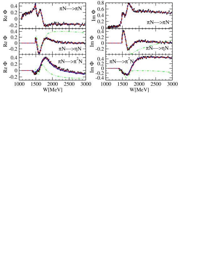
(a) S11 wave

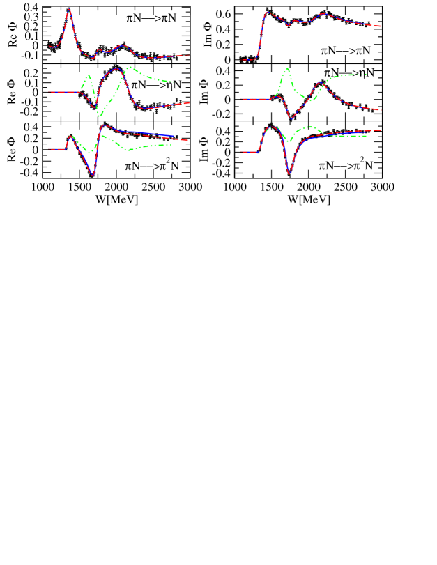
(b) P11 wave

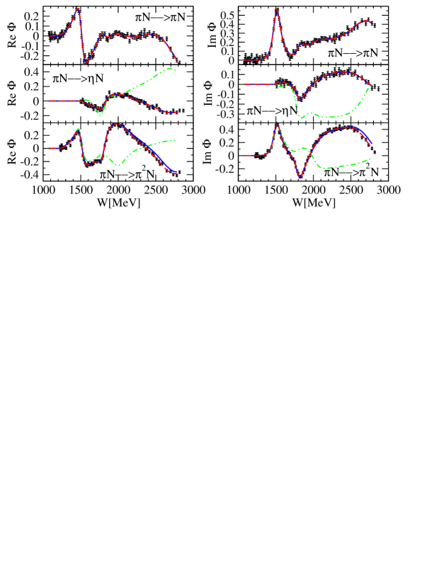
(c) D13 wave

Figure 4: (Color online) The input data sets together with our fit to them with the standard model are shown for the S₁₁, $P_{11}$ and $D_{13}$ partial waves T-matrices.

Table 1: The original parameters of the Zagreb solution for the S₁₁, P₁₁ and D₁₃ partial waves.

Partial	Bare poles				Dressed poles
waves	$\mathrm{W_{s_{1}}}$	$\mathrm{W_{s_{2}}}$	$\mathrm{W_{s_{3}}}$	$\mathrm{W_{s_{4}}}$	$\begin{pmatrix}\mathrm{ReW}\\ \mathrm{-2ImW}\end{pmatrix}$	$\begin{pmatrix}\mathrm{ReW}\\ \mathrm{-2ImW}\end{pmatrix}$	$\begin{pmatrix}\mathrm{ReW}\\ \mathrm{-2ImW}\end{pmatrix}$	$\begin{pmatrix}\mathrm{ReW}\\ \mathrm{-2ImW}\end{pmatrix}$
		$\mathrm{MeV}$				$\mathrm{MeV}$
S11	1523	1640	1837		$\begin{pmatrix}1518\\ 191\end{pmatrix}$	$\begin{pmatrix}1642\\ 205\end{pmatrix}$	$\begin{pmatrix}1784\\ 424\end{pmatrix}$
P11	1607	1771	2186	2852	$\begin{pmatrix}1360\\ 161\end{pmatrix}$	$\begin{pmatrix}1708\\ 175\end{pmatrix}$	$\begin{pmatrix}1728\\ 138\end{pmatrix}$	$\begin{pmatrix}2114\\ 345\end{pmatrix}$
D13	1582	1880	2497		$\begin{pmatrix}1507\\ 121\end{pmatrix}$	$\begin{pmatrix}1805\\ 128\end{pmatrix}$	$\begin{pmatrix}1942\\ 471\end{pmatrix}$	$\begin{pmatrix}2699\\ 558\end{pmatrix}$

Table 2: The stability of the fitting result for the S₁₁ partial wave.

	Number of   channels	Number of    resonances	Fitted   channels	Bare poles			Dressed poles
				$\mathrm{W_{s_{1}}}$	$\mathrm{W_{s_{2}}}$	$\mathrm{W_{s_{3}}}$	$\begin{pmatrix}\mathrm{ReW}\\ \mathrm{-2ImW}\end{pmatrix}$	$\begin{pmatrix}\mathrm{ReW}\\ \mathrm{-2ImW}\end{pmatrix}$	$\begin{pmatrix}\mathrm{ReW}\\ \mathrm{-2ImW}\end{pmatrix}$	$\mathrm{\chi_{R}^{2}}$	$\mathrm{{}^{tot}\chi_{R}^{2}}$
					$\mathrm{MeV}$			$\mathrm{MeV}$
Fit 1	3	3	1	1455	1654	2860	$\begin{pmatrix}1562\\ 100\end{pmatrix}$	$\begin{pmatrix}1684\\ 179\end{pmatrix}$	$\begin{pmatrix}4090\\ 2450\end{pmatrix}$	1.094	117.186
Fit 2	3	3	2	1522	1635	1823	$\begin{pmatrix}1516\\ 185\end{pmatrix}$	$\begin{pmatrix}1640\\ 207\end{pmatrix}$	$\begin{pmatrix}1790\\ 435\end{pmatrix}$	1.004	1.711
$\begin{array}[]{l}Standard\\ fit\end{array}$	3	3	3	1523	1640	1834	$\begin{pmatrix}1518\\ 189\end{pmatrix}$	$\begin{pmatrix}1642\\ 208\end{pmatrix}$	$\begin{pmatrix}1779\\ 427\end{pmatrix}$	1.016	1.016

Table 3: The stability of the fitting result for the P₁₁ partial wave.

	Number of   channels	Number of    resonances	Fitted   channels	Bare poles				Dressed poles
				$\mathrm{W_{s_{1}}}$	$\mathrm{W_{s_{2}}}$	$\mathrm{W_{s_{3}}}$	$\mathrm{W_{s_{4}}}$	$\begin{pmatrix}\mathrm{ReW}\\ \mathrm{-2ImW}\end{pmatrix}$	$\begin{pmatrix}\mathrm{ReW}\\ \mathrm{-2ImW}\end{pmatrix}$	$\begin{pmatrix}\mathrm{ReW}\\ \mathrm{-2ImW}\end{pmatrix}$	$\begin{pmatrix}\mathrm{ReW}\\ \mathrm{-2ImW}\end{pmatrix}$	$\mathrm{\chi_{R}^{2}}$	$\mathrm{{}^{tot}\chi_{R}^{2}}$
					$\mathrm{MeV}$				$\mathrm{MeV}$
Fit 1	3	4	1	1712	1781	2172	3162	$\begin{pmatrix}1416\\ 69\end{pmatrix}$	$\begin{pmatrix}1701\\ 30\end{pmatrix}$	$\begin{pmatrix}1788\\ 128\end{pmatrix}$	$\begin{pmatrix}2118\\ 321\end{pmatrix}$	0.872	99.866
Fit 2	3	4	2	1734	1923	2191	2330	$\begin{pmatrix}1360\\ 169\end{pmatrix}$	$\begin{pmatrix}1695\\ 216\end{pmatrix}$	$\begin{pmatrix}1745\\ 112\end{pmatrix}$	$\begin{pmatrix}2120\\ 350\end{pmatrix}$	1.048	1.739
$\begin{array}[]{l}Standard\\ fit\end{array}$	3	4	3	1607	1772	2182	2841	$\begin{pmatrix}1365\\ 157\end{pmatrix}$	$\begin{pmatrix}1708\\ 174\end{pmatrix}$	$\begin{pmatrix}1731\\ 136\end{pmatrix}$	$\begin{pmatrix}2117\\ 345\end{pmatrix}$	0.958	0.958

Table 4: The stability of the fitting result for the D₁₃ partial wave.

	Number of   channels	Number of    resonances	Fitted   channels	Bare poles			Dressed poles
				$\mathrm{W_{s_{1}}}$	$\mathrm{W_{s_{2}}}$	$\mathrm{W_{s_{3}}}$	$\begin{pmatrix}\mathrm{ReW}\\ \mathrm{-2ImW}\end{pmatrix}$	$\begin{pmatrix}\mathrm{ReW}\\ \mathrm{-2ImW}\end{pmatrix}$	$\begin{pmatrix}\mathrm{ReW}\\ \mathrm{-2ImW}\end{pmatrix}$	$\begin{pmatrix}\mathrm{ReW}\\ \mathrm{-2ImW}\end{pmatrix}$	$\mathrm{\chi_{R}^{2}}$	$\mathrm{{}^{tot}\chi_{R}^{2}}$
					$\mathrm{MeV}$			$\mathrm{MeV}$
Fit 1	3	3	1	1589	1998	2537	$\begin{pmatrix}1500\\ 127\end{pmatrix}$	$\begin{pmatrix}1765\\ 200\end{pmatrix}$	$\begin{pmatrix}1980\\ 232\end{pmatrix}$	$\begin{pmatrix}2720\\ 597\end{pmatrix}$	1.295	137.071
Fit 2	3	3	2	1589	1880	2557	$\begin{pmatrix}1507\\ 127\end{pmatrix}$	$\begin{pmatrix}1800\\ 126\end{pmatrix}$	$\begin{pmatrix}1932\\ 508\end{pmatrix}$	$\begin{pmatrix}2700\\ 595\end{pmatrix}$	1.070	1.555
$\begin{array}[]{l}Standard\\ fit\end{array}$	3	3	3	1582	1880	2499	$\begin{pmatrix}1506\\ 121\end{pmatrix}$	$\begin{pmatrix}1807\\ 127\end{pmatrix}$	$\begin{pmatrix}1939\\ 485\end{pmatrix}$	$\begin{pmatrix}2691\\ 583\end{pmatrix}$	1.027	1.027

V.2 The form of the channel propagator $\Phi(s)$

The major assumption of the CMB model is done about the functional form of the channel propagator. We first define the channel-resonance vertex function in Eq. (2), and then combine it with the phase space factors into the analytic channel propagator, see Eq. (9). We take over a recipe extensively used by CMB group Cut79 , and the full definitions are given by Eqs. (2, 9 and 10).

However, it is very difficult to justify the correctness of these assumptions. So, instead of defending its physical reasonability, and discussing the dependence of the vertex function upon the channel resonance vertex constants $Q_{1a}$ and $Q_{2a}$, we shall test how sensitive our model is substantial but artificial changes of its constituent parts: asymptotic part, intermediate part, threshold behavior.
Procedure
(i) We have chosen the modification function completely artificially, requiring that the change of the channel propagator is localized only to its constituent part, and that the transition from the modified to non-modified part is smooth.
(ii) The imaginary part of the channel propagator is evaluated.
(iii) The real part of the channel propagator is calculated using the dispersion relation given by Eq. (10).
(iv) The input data set is refitted with modified channel propagator.

Important:
We have modified all three channel propagators simultaneously using the same modification function.

V.2.1 Asymptotic part

The imaginary part of the channel propagator was kept unchanged at $s$ below 10 GeV². Above 10 GeV² the correction function g(s) which changes the asymptotic behavior of the channel propagator is introduced:

$$f(s)=f_{0}+f_{1}\cdot e^{-\lambda\cdot(s-s_{0})^{2}},$$ (16)

Modified imaginary part of the channel propagator (omitting channel indices) now reads:

$${\mathrm{I}m}\Phi_{corr}=\left\{{}^{{\mathrm{I}m}\Phi(s){\rm\ \ \ for\ s\leq 10\ GeV^{2}}}_{{\mathrm{I}m}\Phi(s)\cdot f(s){\rm\ \ \ for\ s>10\ GeV^{2}}}\right.$$ (17)

Parameters $f_{0}$, $f_{1}$ and $\lambda$ are determined in such a way to ensure continuity of channel propagator and its first derivative at $s=10$ GeV², and $s=10.5$ GeV². Imaginary and real parts of channel propagator are shown in the Fig. (5) for several values of parameter $f_{0}$.

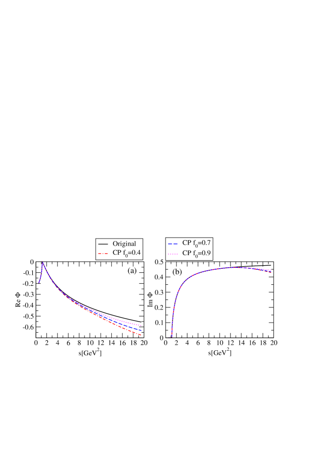
Figure 5: (Color online) Real and imaginary part of channel propagator. Several values of parameter $f_{0}$ are used: $0.4$, $0.7$ and $0.9$.

Let us briefly discuss the analyticity and unitarity of afore used piecewise defined functions. When analyticity of the channel propagator is imposed via dispersion relations, the analyticity of real and imaginary parts themselves is not required Analyticity-piecewise . Piecewise defined imaginary part of channel propagator is by construction a continuous function having continuous first derivative and not necessarily analytic, but when we use dispersion relations to obtain the corresponding real part, we automatically construct the analytic function having the same cut. The idea of the paper is to analyze how this change influences pole position of the T-matrix.

Such a change does not influence unitarity, because in ref. Cut79 it has been explicitly shown that the CMB formalism by the very construction retains unitary if all used functions are analytic.

Result:

As it is seen in Fig. (5) neither imaginary nor real part of the channel propagator are changed in the relevant energy range s $\leq$ 10 GeV².

Conclusion:

Pole positions are unaffected.

V.2.2 Intermediate part

As the intermediate part of the channel propagator, we define the energy domain which is notably above threshold, but not exceeding the high energy part above 10 GeV². In this energy range, 1 GeV${}^{2}<$ $s$ $<$ 10 GeV², most of the known nucleon resonances are situated.

In this part of our analysis channel propagator is multiplied by a function

$$g(s)=\left[\frac{1+a\cdot s+s^{2}}{1+s^{2}}\right]^{2}$$ (18)

which changes a shape of channel propagator without changing its asymptotic or threshold behavior. Depending on the size and the sign of the free parameter $a$, the value of the channel propagator in the intermediate range 2 GeV${}^{2}<$ $s$ $<$ 5 GeV² can be enhanced, or reduced for as much as 100%.

The imaginary part of channel propagator is given by

$$\mathrm{Im}\ \Phi_{corr}=\mathrm{Im}\ \Phi\cdot g(s),$$ (19)

and the real part is calculated using the dispersion relation (10).

The change of the channel propagator for the S₁₁, P₁₁ and D₁₃ partial wave is given in Fig. (6).

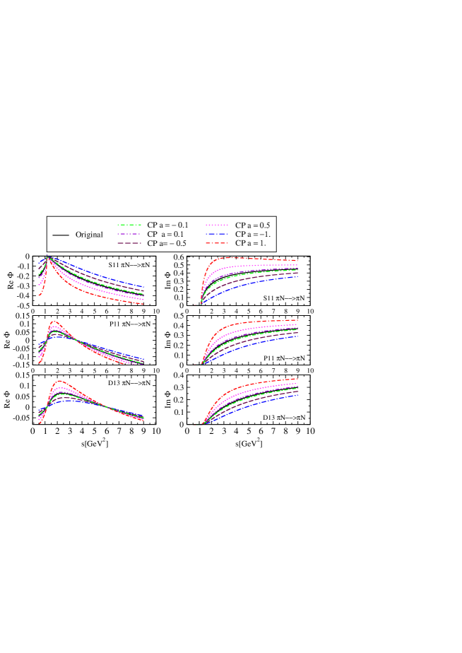
Figure 6: (Color online) Real and imaginary parts of S₁₁, $P_{11}$ and $D_{13}$ elastic channel propagator. We change intermediate part of channel propagator.

Result:

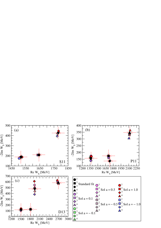
Figure 7: (Color online) The extracted S₁₁, $P_{11}$ and $D_{13}$ partial waves T-matrix poles using different solutions of channel propagator. We change intermediate part of channel propagator and the modification is the same for all three used channels. Red arrows indicate the position of Standard solution poles.

The shift in pole positions for partial waves S₁₁, P₁₁ and D₁₃ are presented in Tables 5- 7 and depicted in Fig.(7).

Table 5: The extracted S₁₁ partial wave T-matrix poles using different solutions of channel propagator. We change intermediate part of channel propagator and the modification is the same for all three used channels

	Bare poles			Dressed poles
Solutions	$\mathrm{W_{s_{1}}}$	$\mathrm{W_{s_{2}}}$	$\mathrm{W_{s_{3}}}$	$\begin{pmatrix}\mathrm{ReW}\\ \mathrm{-2ImW}\end{pmatrix}$	$\begin{pmatrix}\mathrm{ReW}\\ \mathrm{-2ImW}\end{pmatrix}$	$\begin{pmatrix}\mathrm{ReW}\\ \mathrm{-2ImW}\end{pmatrix}$	$\mathrm{\chi_{R}^{2}}$
		$\mathrm{MeV}$			$\mathrm{MeV}$
Sol $a=-1.0$	1522	1640	1837	$\begin{pmatrix}1505\\ 176\end{pmatrix}$	$\begin{pmatrix}1636\\ 208\end{pmatrix}$	$\begin{pmatrix}1773\\ 394\end{pmatrix}$	1.198
Sol $a=-0.5$	1523	1641	1835	$\begin{pmatrix}1512\\ 181\end{pmatrix}$	$\begin{pmatrix}1640\\ 208\end{pmatrix}$	$\begin{pmatrix}1776\\ 418\end{pmatrix}$	1.048
Sol $a=-0.1$	1523	1640	1834	$\begin{pmatrix}1516\\ 188\end{pmatrix}$	$\begin{pmatrix}1642\\ 207\end{pmatrix}$	$\begin{pmatrix}1779\\ 424\end{pmatrix}$	1.031
Standard fit	1523	1640	1834	$\begin{pmatrix}1518\\ 189\end{pmatrix}$	$\begin{pmatrix}1642\\ 208\end{pmatrix}$	$\begin{pmatrix}1779\\ 427\end{pmatrix}$	1.016
Sol $a=0.1$	1523	1640	1834	$\begin{pmatrix}1518\\ 189\end{pmatrix}$	$\begin{pmatrix}1642\\ 207\end{pmatrix}$	$\begin{pmatrix}1780\\ 427\end{pmatrix}$	1.037
Sol $a=0.5$	1523	1639	1833	$\begin{pmatrix}1522\\ 190\end{pmatrix}$	$\begin{pmatrix}1644\\ 207\end{pmatrix}$	$\begin{pmatrix}1782\\ 433\end{pmatrix}$	1.062
Sol $a=1.0$	1523	1638	1831	$\begin{pmatrix}1524\\ 187\end{pmatrix}$	$\begin{pmatrix}1645\\ 210\end{pmatrix}$	$\begin{pmatrix}1783\\ 445\end{pmatrix}$	1.105

Table 6: The extracted P₁₁ partial wave T-matrix poles using different solutions of channel propagator. We change intermediate part of channel propagator and the modification is the same for all three used channels

	Bare poles				Dressed poles
Solutions	$\mathrm{W_{s_{1}}}$	$\mathrm{W_{s_{2}}}$	$\mathrm{W_{s_{3}}}$	$\mathrm{W_{s_{4}}}$	$\begin{pmatrix}\mathrm{ReW}\\ \mathrm{-2ImW}\end{pmatrix}$	$\begin{pmatrix}\mathrm{ReW}\\ \mathrm{-2ImW}\end{pmatrix}$	$\begin{pmatrix}\mathrm{ReW}\\ \mathrm{-2ImW}\end{pmatrix}$	$\begin{pmatrix}\mathrm{ReW}\\ \mathrm{-2ImW}\end{pmatrix}$	$\mathrm{\chi_{R}^{2}}$
		$\mathrm{MeV}$				$\mathrm{MeV}$
Sol $a=-1.0$	1603	1772	2181	2929	$\begin{pmatrix}1367\\ 139\end{pmatrix}$	$\begin{pmatrix}1711\\ 160\end{pmatrix}$	$\begin{pmatrix}1736\\ 139\end{pmatrix}$	$\begin{pmatrix}2105\\ 304\end{pmatrix}$	1.137
Sol $a=-0.5$	1606	1772	2182	2874	$\begin{pmatrix}1367\\ 141\end{pmatrix}$	$\begin{pmatrix}1710\\ 170\end{pmatrix}$	$\begin{pmatrix}1733\\ 137\end{pmatrix}$	$\begin{pmatrix}2111\\ 328\end{pmatrix}$	0.971
Sol $a=-0.1$	1606	1772	2182	2849	$\begin{pmatrix}1359\\ 161\end{pmatrix}$	$\begin{pmatrix}1708\\ 174\end{pmatrix}$	$\begin{pmatrix}1731\\ 137\end{pmatrix}$	$\begin{pmatrix}2115\\ 345\end{pmatrix}$	0.955
Standard fit	1607	1772	2182	2841	$\begin{pmatrix}1365\\ 157\end{pmatrix}$	$\begin{pmatrix}1708\\ 174\end{pmatrix}$	$\begin{pmatrix}1731\\ 136\end{pmatrix}$	$\begin{pmatrix}2117\\ 345\end{pmatrix}$	0.958
Sol $a=0.1$	1606	1772	2182	2796	$\begin{pmatrix}1367\\ 168\end{pmatrix}$	$\begin{pmatrix}1711\\ 168\end{pmatrix}$	$\begin{pmatrix}1732\\ 136\end{pmatrix}$	$\begin{pmatrix}2115\\ 338\end{pmatrix}$	1.001
Sol $a=0.5$	1607	1772	2184	2811	$\begin{pmatrix}1369\\ 173\end{pmatrix}$	$\begin{pmatrix}1707\\ 174\end{pmatrix}$	$\begin{pmatrix}1730\\ 135\end{pmatrix}$	$\begin{pmatrix}2121\\ 343\end{pmatrix}$	0.973
Sol $a=1.0$	1607	1772	2186	2784	$\begin{pmatrix}1374\\ 169\end{pmatrix}$	$\begin{pmatrix}1707\\ 175\end{pmatrix}$	$\begin{pmatrix}1730\\ 135\end{pmatrix}$	$\begin{pmatrix}2127\\ 362\end{pmatrix}$	0.995

Table 7: The extracted D₁₃ partial wave T-matrix poles using different solutions of channel propagator. We change intermediate part of channel propagator and the modification is the same for all three used channels

	Bare poles			Dressed poles
Solutions	$\mathrm{W_{s_{1}}}$	$\mathrm{W_{s_{2}}}$	$\mathrm{W_{s_{3}}}$	$\begin{pmatrix}\mathrm{ReW}\\ \mathrm{-2ImW}\end{pmatrix}$	$\begin{pmatrix}\mathrm{ReW}\\ \mathrm{-2ImW}\end{pmatrix}$	$\begin{pmatrix}\mathrm{ReW}\\ \mathrm{-2ImW}\end{pmatrix}$	$\begin{pmatrix}\mathrm{ReW}\\ \mathrm{-2ImW}\end{pmatrix}$	$\chi_{R}^{2}$
		$\mathrm{MeV}$			$\mathrm{MeV}$
Sol $a=-1.0$	1578	1881	2503	$\begin{pmatrix}1502\\ 106\end{pmatrix}$	$\begin{pmatrix}1806\\ 123\end{pmatrix}$	$\begin{pmatrix}1937\\ 384\end{pmatrix}$	$\begin{pmatrix}2675\\ 583\end{pmatrix}$	1.396
Sol $a=-0.5$	1579	1881	2500	$\begin{pmatrix}1504\\ 113\end{pmatrix}$	$\begin{pmatrix}1807\\ 125\end{pmatrix}$	$\begin{pmatrix}1943\\ 436\end{pmatrix}$	$\begin{pmatrix}2692\\ 567\end{pmatrix}$	1.087
Sol $a=-0.1$	1581	1880	2498	$\begin{pmatrix}1505\\ 120\end{pmatrix}$	$\begin{pmatrix}1808\\ 127\end{pmatrix}$	$\begin{pmatrix}1941\\ 479\end{pmatrix}$	$\begin{pmatrix}2697\\ 575\end{pmatrix}$	1.027
Standard fit	1582	1880	2499	$\begin{pmatrix}1506\\ 121\end{pmatrix}$	$\begin{pmatrix}1807\\ 127\end{pmatrix}$	$\begin{pmatrix}1939\\ 485\end{pmatrix}$	$\begin{pmatrix}2691\\ 583\end{pmatrix}$	1.027
Sol $a=0.1$	1582	1879	2497	$\begin{pmatrix}1505\\ 121\end{pmatrix}$	$\begin{pmatrix}1808\\ 127\end{pmatrix}$	$\begin{pmatrix}1939\\ 500\end{pmatrix}$	$\begin{pmatrix}2685\\ 594\end{pmatrix}$	1.032
Sol $a=0.5$	1584	1878	2495	$\begin{pmatrix}1506\\ 127\end{pmatrix}$	$\begin{pmatrix}1808\\ 127\end{pmatrix}$	$\begin{pmatrix}1935\\ 546\end{pmatrix}$	$\begin{pmatrix}2670\\ 609\end{pmatrix}$	1.084
Sol $a=1.0$	1585	1876	2493	$\begin{pmatrix}1507\\ 135\end{pmatrix}$	$\begin{pmatrix}1811\\ 127\end{pmatrix}$	$\begin{pmatrix}1929\\ 610\end{pmatrix}$	$\begin{pmatrix}2656\\ 627\end{pmatrix}$	1.183

Conclusions:

As seen in Fig. (6) changing the $a$ parameter in ad hoc modification function given by Eq. (18) within the range -1 $<$ $a$ $<$ 1 changes the imaginary part of the channel propagator for up to 100% in the intermediate range 2 $GeV^{2}$ $<$ $s$ $<$ 5 GeV².

We observe:

1. The strong modification of the imaginary part of the channel propagator is via the dispersion relation Eq. (10) transmitted to the real part, causing opposite effect (reduction) for the S-wave, and a combined effect for other partial waves.

2. From Tables 5- 7 we learn that bare poles are fairly stable with respect with change of the intermediate part of the channel propagator, while dressed poles experience quite a change.

3. The dressed poles can, however, be classified in two categories:

   a.

   Poles weekly dependent upon the strong changes of the intermediate part - stable poles
   S₁₁ (1518), S₁₁ (1642), P₁₁ (1731), D₁₃ (1506) and D₁₃ (1807)

   b.

   Poles moderately and notably dependent upon the strong changes of the intermediate part - running poles
   S₁₁ (1779), $P_{11}(1365)$, P₁₁ (1731), P₁₁ (2117), D₁₃ (1939) and D₁₃ (2691)

4. We may connect the category of the pole to its self energy content:

   a.

   For the stable poles the self energy correction to the bare mass is small

   b.

   For the running poles, the self energy correction to the bare mass is either strong (as for S₁₁ (1779), P₁₁ (1731), P₁₁ (2117) and D₁₃ (2691) ), or poles are entirely dynamically generated meaning that they do not at all have a corresponding, nearby bare poles (as for $P_{11}(1365)$ Roper resonance, and D₁₃ (1939) )

5. Consequently, “difference” of bare and dressed pole position can be taken as the criterion for the stability of the pole position with respect to the strong modification of the intermediate part: “The lower the self energy correction is, the more stable the pole position is.”

6. As seen in Tables 5 - 7, the reduced $\chi^{2}_{R}$, the quantity representing the measure of ability of our model to reproduce the input data, is systematically smallest for the non-modified solution. In other words, our fit to the input data worsens whenever any change to the intermediate part of channel propagator is introduced.

V.2.3 Threshold behavior

In this part of our analysis, behavior of channel propagator’s imaginary part close to the threshold a given channel is changed. For values $s$ $>$ 3.5 GeV² channel propagator is kept unchanged. The threshold behavior of imaginary part of the channel propagator is given by $q^{2L+1}$. It is changed by multiplying the channel propagator with $q^{\lambda}$. The continuity in energy is ensured by the matching function $h(s)=(a+b\cdot s+c\cdot s^{2})$. Modified imaginary part is given by:

$$\mathrm{Im}\Phi_{corr}=\mathrm{Im}\Phi\cdot q_{a}^{\lambda}\cdot h(s).$$ (20)

with $\lambda=\pm 0.5$. Parameters $a$, $b$ and $c$ are adjusted in such a way to ensure continuity of channel propagator and first derivative at $s$ =3.5 GeV² .
The change of the channel propagator for the S₁₁, P₁₁ and D₁₃ partial wave is given in Fig. (8).

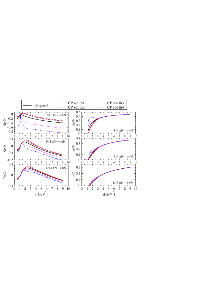
Figure 8: (Color online) Real and imaginary parts of the $S_{11}$, $P_{11}$ and $D_{13}$ elastic channel propagator. Threshold behavior. Sol th1: $\mathrm{Im}\Phi_{corr}=\mathrm{Im}\Phi\cdot\sqrt{q}(a+cs^{2})$, Sol th2: $\mathrm{Im}\Phi_{corr}=\mathrm{Im}\Phi\cdot\sqrt{q}(a+0.5s+cs^{2})$, Sol th3: $\mathrm{Im}\Phi_{corr}=\mathrm{Im}\Phi\cdot(\frac{1}{\sqrt{q}})(a+cs^{2})$, Sol th4: $\mathrm{Im}\Phi_{corr}=\mathrm{Im}\Phi\cdot(\frac{1}{\sqrt{q}})(a-0.5s+cs^{2})$.

Result:

The shift in pole positions for partial waves S₁₁, P₁₁ and D₁₃ are presented in Tables 8- 10 and depicted in Fig. (9).  We personally do not believe that such strong variations in the threshold behavior are physics-wise permissible, but we have investigated this aspect of our model just to check the how quickly our results deteriorate when even uphysical changes are introduced. We are happy to conclude that the results are only moderately sensitive to even huge changes.

Table 8: The extracted $S_{11}$ partial wave T-matrix poles using different solutions of channel propagator. We change threshold behavior of channel propagator and the modification is the same for all three used channels.

	Bare poles			Dressed poles
Solutions	$\mathrm{W_{s_{1}}}$	$\mathrm{W_{s_{2}}}$	$\mathrm{W_{s_{3}}}$	$\begin{pmatrix}\mathrm{ReW}\\ \mathrm{-2ImW}\end{pmatrix}$	$\begin{pmatrix}\mathrm{ReW}\\ \mathrm{-2ImW}\end{pmatrix}$	$\begin{pmatrix}\mathrm{ReW}\\ \mathrm{-2ImW}\end{pmatrix}$	$\mathrm{\chi_{R}^{2}}$
		$\mathrm{MeV}$			$\mathrm{MeV}$
Standard fit	1523	1640	1834	$\begin{pmatrix}1518\\ 189\end{pmatrix}$	$\begin{pmatrix}1642\\ 208\end{pmatrix}$	$\begin{pmatrix}1779\\ 427\end{pmatrix}$	1.016
Sol th1	1551	1673	1899	$\begin{pmatrix}1505\\ 139\end{pmatrix}$	$\begin{pmatrix}1642\\ 212\end{pmatrix}$	$\begin{pmatrix}1755\\ 468\end{pmatrix}$	1.289
Sol th2	1557	1683	1915	$\begin{pmatrix}1505\\ 130\end{pmatrix}$	$\begin{pmatrix}1642\\ 208\end{pmatrix}$	$\begin{pmatrix}1751\\ 457\end{pmatrix}$	1.372
Sol th3	1477	1575	1728	$\begin{pmatrix}1552\\ 164\end{pmatrix}$	$\begin{pmatrix}1642\\ 212\end{pmatrix}$	$\begin{pmatrix}1781\\ 397\end{pmatrix}$	1.409
Sol th4	1453	1540	1678	$\begin{pmatrix}1557\\ 154\end{pmatrix}$	$\begin{pmatrix}1643\\ 203\end{pmatrix}$	$\begin{pmatrix}1786\\ 401\end{pmatrix}$	1.587

Table 9: The extracted $P_{11}$ partial wave T-matrix poles using different solutions of channel propagator. We change threshold behavior of channel propagator and the modification is the same for all three used channels

	Bare poles				Dressed poles
Solutions	$\mathrm{W_{s_{1}}}$	$\mathrm{W_{s_{2}}}$	$\mathrm{W_{s_{3}}}$	$\mathrm{W_{s_{4}}}$	$\begin{pmatrix}\mathrm{ReW}\\ \mathrm{-2ImW}\end{pmatrix}$	$\begin{pmatrix}\mathrm{ReW}\\ \mathrm{-2ImW}\end{pmatrix}$	$\begin{pmatrix}\mathrm{ReW}\\ \mathrm{-2ImW}\end{pmatrix}$	$\begin{pmatrix}\mathrm{ReW}\\ \mathrm{-2ImW}\end{pmatrix}$	$\mathrm{\chi_{R}^{2}}$
		$\mathrm{MeV}$				$\mathrm{MeV}$
Standard fit	1607	1772	2182	2841	$\begin{pmatrix}1365\\ 157\end{pmatrix}$	$\begin{pmatrix}1708\\ 174\end{pmatrix}$	$\begin{pmatrix}1731\\ 136\end{pmatrix}$	$\begin{pmatrix}2117\\ 345\end{pmatrix}$	0.957
Sol th1	1629	1780	2192	2802	$\begin{pmatrix}1376\\ 161\end{pmatrix}$	$\begin{pmatrix}1705\\ 168\end{pmatrix}$	$\begin{pmatrix}1733\\ 128\end{pmatrix}$	$\begin{pmatrix}2112\\ 327\end{pmatrix}$	1.157
Sol th2	1639	1784	2196	2801	$\begin{pmatrix}1383\\ 163\end{pmatrix}$	$\begin{pmatrix}1706\\ 164\end{pmatrix}$	$\begin{pmatrix}1734\\ 124\end{pmatrix}$	$\begin{pmatrix}2112\\ 323\end{pmatrix}$	1.335
Sol th3	1572	1763	2174	2712	$\begin{pmatrix}1351\\ 163\end{pmatrix}$	$\begin{pmatrix}1715\\ 175\end{pmatrix}$	$\begin{pmatrix}1729\\ 143\end{pmatrix}$	$\begin{pmatrix}2123\\ 352\end{pmatrix}$	1.010
Sol th4	1534	1753	2168	2546	$\begin{pmatrix}1341\\ 148\end{pmatrix}$	$\begin{pmatrix}1718\\ 191\end{pmatrix}$	$\begin{pmatrix}1724\\ 145\end{pmatrix}$	$\begin{pmatrix}2135\\ 344\end{pmatrix}$	1.274

Table 10: The extracted $D_{13}$ partial wave T-matrix poles using different solution of channel propagator. We change threshold behavior of channel propagator and the modification is the same for all three used channels

	Bare poles			Dressed poles
Solutions	$\mathrm{W_{s_{1}}}$	$\mathrm{W_{s_{2}}}$	$\mathrm{W_{s_{3}}}$	$\begin{pmatrix}\mathrm{ReW}\\ \mathrm{-2ImW}\end{pmatrix}$	$\begin{pmatrix}\mathrm{ReW}\\ \mathrm{-2ImW}\end{pmatrix}$	$\begin{pmatrix}\mathrm{ReW}\\ \mathrm{-2ImW}\end{pmatrix}$	$\begin{pmatrix}\mathrm{ReW}\\ \mathrm{-2ImW}\end{pmatrix}$	$\chi_{R}^{2}$
		$\mathrm{MeV}$			$\mathrm{MeV}$
Standard fit	1582	1880	2499	$\begin{pmatrix}1506\\ 121\end{pmatrix}$	$\begin{pmatrix}1807\\ 127\end{pmatrix}$	$\begin{pmatrix}1939\\ 485\end{pmatrix}$	$\begin{pmatrix}2691\\ 583\end{pmatrix}$	1.027
Sol th1	1589	1881	2500	$\begin{pmatrix}1503\\ 114\end{pmatrix}$	$\begin{pmatrix}1807\\ 124\end{pmatrix}$	$\begin{pmatrix}1933\\ 449\end{pmatrix}$	$\begin{pmatrix}2694\\ 567\end{pmatrix}$	1.057
Sol th2	1593	1882	2505	$\begin{pmatrix}1502\\ 109\end{pmatrix}$	$\begin{pmatrix}1806\\ 123\end{pmatrix}$	$\begin{pmatrix}1930\\ 424\end{pmatrix}$	$\begin{pmatrix}2692\\ 563\end{pmatrix}$	1.148
Sol th3	1573	1875	2481	$\begin{pmatrix}1508\\ 128\end{pmatrix}$	$\begin{pmatrix}1808\\ 129\end{pmatrix}$	$\begin{pmatrix}1947\\ 518\end{pmatrix}$	$\begin{pmatrix}2680\\ 609\end{pmatrix}$	1.119
Sol th4	1563	1871	2468	$\begin{pmatrix}1515\\ 137\end{pmatrix}$	$\begin{pmatrix}1810\\ 132\end{pmatrix}$	$\begin{pmatrix}1961\\ 554\end{pmatrix}$	$\begin{pmatrix}2662\\ 648\end{pmatrix}$	1.363

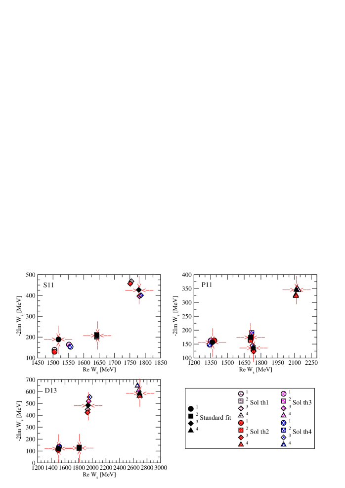
Figure 9: (Color online) The extracted S₁₁, $P_{11}$ and D₁₃ partial waves T-matrix poles using different solutions of channel propagator. We change threshold behavior of channel propagator and the modification is the same for all three used channels. Red arrows indicate the position of Standard solution poles.

Conclusion:

As seen in Fig. (8) the threshold behavior was modified by the continuous and arbitrary function given by Eq. (20). We have chosen 4 possibilities, in two of them the threshold behavior has been made shallower (th1 and th2), and for the two of them (th3 and th4) much steeper.

We observe:

1. The strong modification of the imaginary part threshold behavior of the channel propagator is via the dispersion relation Eq. (10) transmitted to the real part, causing significant changes of the real part in complete energy range.

2. Contrary to the former case when intermediate part of the channel propagator has been analyzed, bare poles now experience significant change for all energies, and all partial waves.

3. Dressing tries to compensate for the strong shift of the bare poles, but not always very successfully.

4. As a result, we conclude that the correct threshold behavior of the channel propagator is essential for the applicability of the model.

5. With some possible coincidental exceptions, all dressed poles experience a notable shift.

6. As seen in Tables 8 - 10, the reduced $\chi^{2}_{R}$, the quantity representing the measure of ability of our model to reproduce the input data, is systematically smallest for the non-modified solution. In other words, our fit to the input data worsen whenever any change to the threshold behavior of channel propagator is introduced.

V.3 Dispersion integral subtraction constant

As positions of bare poles are in principle not too well defined (they must depend on the renormalization scheme, see Capstick et.al CapstickEPJA ), the fact that they can only be significantly moved by changing the threshold behavior troubled us a lot. As our model is an effective model, changing its ingredients should enable us to ”mimic” at least some of other models, and that means we should observe a significant shift of bare poles. So, having the bare pole model dependence hidden only in fairly well defined threshold behavior was non-satisfactory.

The answer to this issue was already hinted by Vrana et al in Vrana2000 where they have shown that position of bare poles significantly depends on the dispersion integral subtraction constant, and its importance for the position of the bare and dressed poles was briefly discussed. We have, therefore, extensively tested this freedom within our model, and shifted the subtraction constant $\mathrm{Re}\Phi(s_{0})$ defined in Eq. (10) from its original zero value. We have chosen SC Sol 1: $\mathrm{Re}\Phi(s_{0})=m_{\pi}$ for all three used channels; SC Sol 2: $\mathrm{Re}\Phi(s_{0})=m_{\pi}$ for $\pi N$ channel only, while in other two channels $\mathrm{Re}\Phi(s_{0})=0$; SC Sol 3: $\mathrm{Re}\Phi(s_{0})=m_{\eta}$ for $\eta N$ channel only, while in other two channels $\mathrm{Re}\Phi(s_{0})=0$; SC Sol 4: $\mathrm{Re}\Phi(s_{0})=m_{\pi^{2}}$ for $\pi^{2}N$ channel only, while in other two channels $\mathrm{Re}\Phi(s_{0})=0$; SC Sol 5: $\mathrm{Re}\Phi(s_{0})=-m_{\pi}$ for all three used channels, SC Sol 6: $\mathrm{Re}\Phi(s_{0})=m_{a}$, where $m_{a}$ is the mass of the meson in corresponding channel.

As changing the dispersion integral subtraction constant only shifts the real part of the channel propagator into positive or negative y-direction for a certain constant value, we show the modified real part of the S₁₁, P₁₁ and D₁₃ partial wave channel propagator in Fig. (10) for only two representative values of subtraction constant $\mathrm{Re}\Phi(s_{0})=\pm m_{\pi}$ in all three channels simultaneously. For other modifications related plots look qualitatively the same, so we do not show them explicitly.

Results:

Results are given in Tables 11 -13 and in Fig. (11).

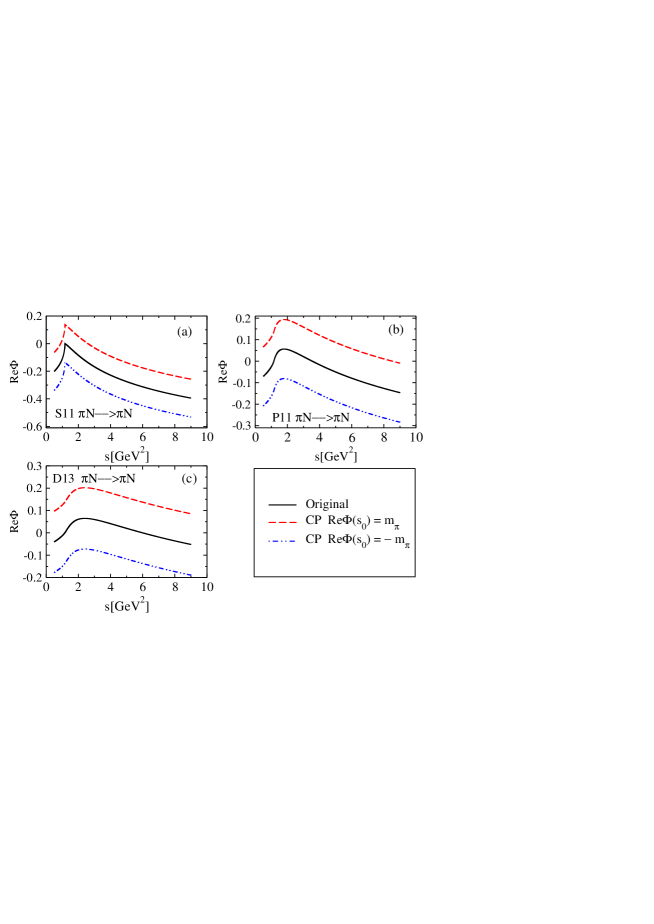
Figure 10: (Color online) Real part of S₁₁, $P_{11}$ and $D_{13}$ elastic channel propagator. We change the dispersion integral subtraction constant.

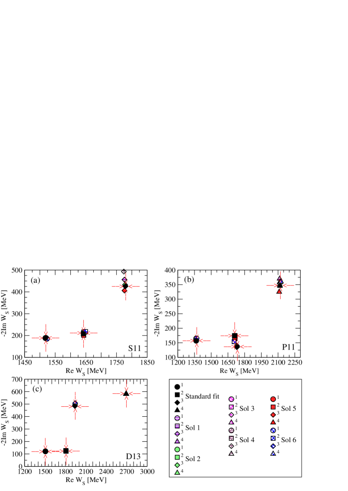
Figure 11: (Color online) The extracted S₁₁, $P_{11}$ and D₁₃ partial waves T-matrix poles using different solutions of channel propagator. We change dispersion integral subtraction constant for all three used channels. Red arrows indicate the position of Standard solution poles.

Table 11: The extracted $S_{11}$ partial wave $T$-matrix poles using different values of subtraction constant. SC Sol 1: $\mathrm{Re}\Phi(s_{0})=m_{\pi}$ for all three used channels; SC Sol 2: $\mathrm{Re}\Phi(s_{0})=m_{\pi}$ for $\pi N$ channel only, while in other two channels $\mathrm{Re}\Phi(s_{0})=0$; SC Sol 3: $\mathrm{Re}\Phi(s_{0})=m_{\eta}$ for $\eta N$ channel only, while in other two channels $\mathrm{Re}\Phi(s_{0})=0$; SC Sol 4: $\mathrm{Re}\Phi(s_{0})=m_{\pi^{2}}$ for $\pi^{2}N$ channel only, while in other two channels $\mathrm{Re}\Phi(s_{0})=0$; SC Sol 5: $\mathrm{Re}\Phi(s_{0})=-m_{\pi}$ for all three used channels, SC Sol 6: $\mathrm{Re}\Phi(s_{0})=m_{a}$, where $m_{a}$ is the mass of the meson in corresponding channel.

	Bare poles			Dressed poles
	$W_{s_{1}}$	$W_{s_{2}}$	$W_{s_{3}}$	$\begin{pmatrix}\mathrm{ReW}\\ \mathrm{-2ImW}\end{pmatrix}$	$\begin{pmatrix}\mathrm{ReW}\\ \mathrm{-2ImW}\end{pmatrix}$	$\begin{pmatrix}\mathrm{ReW}\\ \mathrm{-2ImW}\end{pmatrix}$	$\mathrm{\chi_{R}^{2}}$
		$MeV$			$MeV$
Standard fit	1523	1640	1834	$\begin{pmatrix}1518\\ 189\end{pmatrix}$	$\begin{pmatrix}1642\\ 208\end{pmatrix}$	$\begin{pmatrix}1779\\ 427\end{pmatrix}$	1.016
SC Sol 1	1579	1686	1953	$\begin{pmatrix}1520\\ 188\end{pmatrix}$	$\begin{pmatrix}1643\\ 216\end{pmatrix}$	$\begin{pmatrix}1776\\ 456\end{pmatrix}$	1.054
SC Sol 2	1537	1662	1868	$\begin{pmatrix}1520\\ 189\end{pmatrix}$	$\begin{pmatrix}1642\\ 210\end{pmatrix}$	$\begin{pmatrix}1778\\ 433\end{pmatrix}$	1.019
SC Sol 3	1587	1730	1907	$\begin{pmatrix}1518\\ 188\end{pmatrix}$	$\begin{pmatrix}1642\\ 207\end{pmatrix}$	$\begin{pmatrix}1779\\ 425\end{pmatrix}$	1.016
SC Sol 4	1529	1659	2150	$\begin{pmatrix}1522\\ 186\end{pmatrix}$	$\begin{pmatrix}1647\\ 216\end{pmatrix}$	$\begin{pmatrix}1774\\ 493\end{pmatrix}$	1.141
SC Sol 5	1462	1593	1756	$\begin{pmatrix}1518\\ 188\end{pmatrix}$	$\begin{pmatrix}1643\\ 201\end{pmatrix}$	$\begin{pmatrix}1776\\ 406\end{pmatrix}$	1.052
SC Sol 6	1663	1761	2252	$\begin{pmatrix}1523\\ 185\end{pmatrix}$	$\begin{pmatrix}1649\\ 218\end{pmatrix}$	$\begin{pmatrix}1775\\ 510\end{pmatrix}$	1.216

Table 12: The extracted $P_{11}$ partial wave $T$-matrix poles using different values of subtraction constant. SC Sol 1: $\mathrm{Re}\Phi(s_{0})=m_{\pi}$ for all three used channels; SC Sol 2: $\mathrm{Re}\Phi(s_{0})=m_{\pi}$ for $\pi N$ channel only, while in other two channels $\mathrm{Re}\Phi(s_{0})=0$; SC Sol 3: $\mathrm{Re}\Phi(s_{0})=m_{\eta}$ for $\eta N$ channel only, while in other two channels $\mathrm{Re}\Phi(s_{0})=0$; SC Sol 4: $\mathrm{Re}\Phi(s_{0})=m_{\pi^{2}}$ for $\pi^{2}N$ channel only, while in other two channels $\mathrm{Re}\Phi(s_{0})=0$; SC Sol 5: $\mathrm{Re}\Phi(s_{0})=-m_{\pi}$ for all three used channels, SC Sol 6: $\mathrm{Re}\Phi(s_{0})=m_{a}$, where $m_{a}$ is the mass of the meson in corresponding channel.

	Bare poles				Dressed poles
Solutions	$\mathrm{W_{s_{1}}}$	$\mathrm{W_{s_{2}}}$	$\mathrm{W_{s_{3}}}$	$\mathrm{W_{s_{4}}}$	$\begin{pmatrix}\mathrm{ReW}\\ \mathrm{-2ImW}\end{pmatrix}$	$\begin{pmatrix}\mathrm{ReW}\\ \mathrm{-2ImW}\end{pmatrix}$	$\begin{pmatrix}\mathrm{ReW}\\ \mathrm{-2ImW}\end{pmatrix}$	$\begin{pmatrix}\mathrm{ReW}\\ \mathrm{-2ImW}\end{pmatrix}$	$\mathrm{\chi_{R}^{2}}$
		$\mathrm{MeV}$				$\mathrm{MeV}$
Standard fit	1607	1772	2182	2841	$\begin{pmatrix}1365\\ 157\end{pmatrix}$	$\begin{pmatrix}1708\\ 174\end{pmatrix}$	$\begin{pmatrix}1731\\ 136\end{pmatrix}$	$\begin{pmatrix}2117\\ 345\end{pmatrix}$	0.958
SC Sol 1	1686	1858	2323	4216	$\begin{pmatrix}1365\\ 157\end{pmatrix}$	$\begin{pmatrix}1715\\ 174\end{pmatrix}$	$\begin{pmatrix}1730\\ 135\end{pmatrix}$	$\begin{pmatrix}2114\\ 370\end{pmatrix}$	1.011
SC Sol 2	1660	1801	2191	3279	$\begin{pmatrix}1364\\ 160\end{pmatrix}$	$\begin{pmatrix}1713\\ 173\end{pmatrix}$	$\begin{pmatrix}1730\\ 136\end{pmatrix}$	$\begin{pmatrix}2116\\ 359\end{pmatrix}$	0.965
SC Sol 3	1611	1796	2376	3586	$\begin{pmatrix}1364\\ 159\end{pmatrix}$	$\begin{pmatrix}1711\\ 175\end{pmatrix}$	$\begin{pmatrix}1730\\ 135\end{pmatrix}$	$\begin{pmatrix}2116\\ 349\end{pmatrix}$	0.953
SC Sol 4	1662	1809	2181	4842	$\begin{pmatrix}1364\\ 160\end{pmatrix}$	$\begin{pmatrix}1712\\ 173\end{pmatrix}$	$\begin{pmatrix}1730\\ 136\end{pmatrix}$	$\begin{pmatrix}2116\\ 357\end{pmatrix}$	0.959
SC Sol 5	1461	1634	1966	2412	$\begin{pmatrix}1365\\ 165\end{pmatrix}$	$\begin{pmatrix}1711\\ 164\end{pmatrix}$	$\begin{pmatrix}1731\\ 140\end{pmatrix}$	$\begin{pmatrix}2110\\ 325\end{pmatrix}$	1.027
SC Sol 6	1696	1876	2433	7115	$\begin{pmatrix}1369\\ 165\end{pmatrix}$	$\begin{pmatrix}1706\\ 154\end{pmatrix}$	$\begin{pmatrix}1734\\ 136\end{pmatrix}$	$\begin{pmatrix}2126\\ 360\end{pmatrix}$	1.303

Table 13: The extracted $D_{13}$ partial wave $T$-matrix poles using different values of subtraction constant. SC Sol 1: $\mathrm{Re}\Phi(s_{0})=m_{\pi}$ for all three used channels; SC Sol 2: $\mathrm{Re}\Phi(s_{0})=m_{\pi}$ for $\pi N$ channel only, while in other two channels $\mathrm{Re}\Phi(s_{0})=0$; SC Sol 3: $\mathrm{Re}\Phi(s_{0})=m_{\eta}$ for $\eta N$ channel only, while in other two channels $\mathrm{Re}\Phi(s_{0})=0$; SC Sol 4: $\mathrm{Re}\Phi(s_{0})=m_{\pi^{2}}$ for $\pi^{2}N$ channel only, while in other two channels $\mathrm{Re}\Phi(s_{0})=0$; SC Sol 5: $\mathrm{Re}\Phi(s_{0})=-m_{\pi}$ for all three used channels, SC Sol 6: $\mathrm{Re}\Phi(s_{0})=m_{a}$, where $m_{a}$ is the mass of the meson in corresponding channel.

	Bare poles			Dressed poles
Solutions	$\mathrm{W_{s_{1}}}$	$\mathrm{W_{s_{2}}}$	$\mathrm{W_{s_{3}}}$	$\begin{pmatrix}\mathrm{ReW}\\ \mathrm{-2ImW}\end{pmatrix}$	$\begin{pmatrix}\mathrm{ReW}\\ \mathrm{-2ImW}\end{pmatrix}$	$\begin{pmatrix}\mathrm{ReW}\\ \mathrm{-2ImW}\end{pmatrix}$	$\begin{pmatrix}\mathrm{ReW}\\ \mathrm{-2ImW}\end{pmatrix}$	$\chi_{R}^{2}$
		$\mathrm{MeV}$			$\mathrm{MeV}$
Standard fit	1582	1880	2499	$\begin{pmatrix}1506\\ 121\end{pmatrix}$	$\begin{pmatrix}1807\\ 121\end{pmatrix}$	$\begin{pmatrix}1939\\ 485\end{pmatrix}$	$\begin{pmatrix}2675\\ 583\end{pmatrix}$	1.027
SC Sol 1	1666	1988	2683	$\begin{pmatrix}1506\\ 121\end{pmatrix}$	$\begin{pmatrix}1808\\ 124\end{pmatrix}$	$\begin{pmatrix}1942\\ 497\end{pmatrix}$	$\begin{pmatrix}2691\\ 581\end{pmatrix}$	1.041
SC Sol 2	1619	1891	2547	$\begin{pmatrix}1506\\ 121\end{pmatrix}$	$\begin{pmatrix}1807\\ 127\end{pmatrix}$	$\begin{pmatrix}1939\\ 485\end{pmatrix}$	$\begin{pmatrix}2691\\ 583\end{pmatrix}$	1.031
SC Sol 3	1628	2071	2599	$\begin{pmatrix}1506\\ 122\end{pmatrix}$	$\begin{pmatrix}1807\\ 127\end{pmatrix}$	$\begin{pmatrix}1939\\ 486\end{pmatrix}$	$\begin{pmatrix}2692\\ 583\end{pmatrix}$	1.031
SC Sol 4	1661	1930	2661	$\begin{pmatrix}1506\\ 122\end{pmatrix}$	$\begin{pmatrix}1807\\ 127\end{pmatrix}$	$\begin{pmatrix}1939\\ 486\end{pmatrix}$	$\begin{pmatrix}2692\\ 583\end{pmatrix}$	1.031
SC Sol 5	1317	1697	2376	$\begin{pmatrix}1505\\ 121\end{pmatrix}$	$\begin{pmatrix}1805\\ 125\end{pmatrix}$	$\begin{pmatrix}1939\\ 485\end{pmatrix}$	$\begin{pmatrix}2692\\ 583\end{pmatrix}$	1.032
SC Sol 6	1678	2071	2722	$\begin{pmatrix}1506\\ 121\end{pmatrix}$	$\begin{pmatrix}1810\\ 122\end{pmatrix}$	$\begin{pmatrix}1943\\ 508\end{pmatrix}$	$\begin{pmatrix}2690\\ 580\end{pmatrix}$	1.183

We see that bare pole positions are notably changed with the variation of the dispersion relation subtraction point value. For the shift into the time-like direction the bare poles are shifted upwards; and when the subtraction point is shifted into the negative energy region the value of bare poles is reduced. The change is notable, and for inspected values varies for 150 - 200 MeV. It is important to notice that the dressed pole positions are extremely stable, see Fig. (11), and not influenced by the subtraction constant values.

We have also tested the freedom in choosing the dispersion integral subtraction point point $s_{0}$. In Fig. (12) where the resulting real part is depicted, we show that the results are qualitatively and quantitatively similar to changing the size of the subtraction constant. We see that changing the subtraction point value shifts the real part upwards and downwards depending on the direction of the shift. So, in practice, this freedom is equivalent to retaining the subtraction point at threshold and varying the subtraction constant. Therefore, the similar conclusions as in case of dispersion constant variation are drawn that the bare poles are strongly influenced, and dressed poles remain virtually untouched.

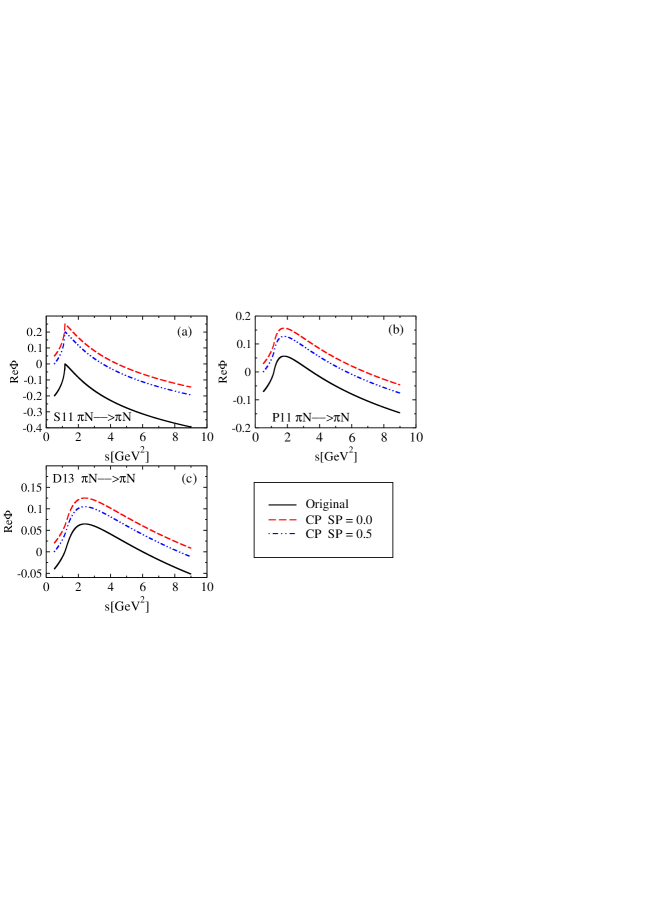
Figure 12: (Color online) Real part of S₁₁, $P_{11}$ and $D_{13}$ elastic channel propagator. We change the dispersion integral subtraction point value.

Conclusion:

Results shown in Tables 11 - 13 prove that the value of subtraction constant affect bare pole positions significantly. Dressed poles remain practically unchanged.

V.4 Background parameterization

Additional background poles below and above physical region are added. Our model was based on the premises that two subthreshold unphysical poles are enough to represent the smooth energy dependent background, and we test this assumption. We test two aspects:

1. Are two poles absolutely essential?

2. Does adding new subthreshold, or distant, positive energy poles change the pole positions?

Therefore, we have added first one, and then two poles, below, and far above threshold, and with different signs representing attraction or repulsion. All possible combinations for three analyzed partial waves are analyzed.

Result:

The shift in pole positions for partial waves S₁₁, P₁₁ and D₁₃ are presented in Tables 14- 16 and depicted in Fig. (13).

Table 14: The extracted $S_{11}$ partial wave T-matrix poles. Additional background poles below and above physical region are added.

	Bare poles					Dressed poles
Solutions	$\begin{array}[]{c}\mathrm{B1}\\ \mathrm{B2}\end{array}$	$\begin{array}[]{c}\mathrm{B3}\\ \mathrm{B4}\end{array}$	$\mathrm{W_{s_{1}}}$	$\mathrm{W_{s_{2}}}$	$\mathrm{W_{s_{3}}}$	$\begin{pmatrix}\mathrm{ReW}\\ \mathrm{-2ImW}\end{pmatrix}$	$\begin{pmatrix}\mathrm{ReW}\\ \mathrm{-2ImW}\end{pmatrix}$	$\begin{pmatrix}\mathrm{ReW}\\ \mathrm{-2ImW}\end{pmatrix}$	$\mathrm{\chi_{R}^{2}}$
	$\mathrm{GeV^{2}}$	$\mathrm{GeV^{2}}$		$\mathrm{MeV}$			$\mathrm{MeV}$
Standard fit	$\begin{array}[]{c}-1.256\\ 0.210\end{array}$		1523	1640	1834	$\begin{pmatrix}1518\\ 189\end{pmatrix}$	$\begin{pmatrix}1642\\ 208\end{pmatrix}$	$\begin{pmatrix}1779\\ 427\end{pmatrix}$	1.016
Sol 1$\begin{array}[]{c}e1=+1(Below)\\ e2=-1(Below)\\ e3=+1(Below)\end{array}$	$\begin{array}[]{c}-1.382\\ 0.460\end{array}$	-1.851	1523	1640	1835	$\begin{pmatrix}1518\\ 189\end{pmatrix}$	$\begin{pmatrix}1642\\ 208\end{pmatrix}$	$\begin{pmatrix}1779\\ 427\end{pmatrix}$	1.016
Sol 2$\begin{array}[]{c}e1=+1(Below)\\ e2=-1(Below)\\ e3=-1(Below)\end{array}$	$\begin{array}[]{c}-2.508\\ -6.794\end{array}$	0.419	1523	1640	1834	$\begin{pmatrix}1518\\ 189\end{pmatrix}$	$\begin{pmatrix}1642\\ 208\end{pmatrix}$	$\begin{pmatrix}1780\\ 427\end{pmatrix}$	1.019
Sol 3$\begin{array}[]{c}e1=+1(Below)\\ e2=-1(Below)\\ e3=-1(Below)\\ e4=+1(Below)\end{array}$	$\begin{array}[]{c}-0.0049\\ 0.103\end{array}$	$\begin{array}[]{c}-1.078\\ -0.0024\end{array}$	1523	1640	1835	$\begin{pmatrix}1520\\ 191\end{pmatrix}$	$\begin{pmatrix}1641\\ 207\end{pmatrix}$	$\begin{pmatrix}1781\\ 420\end{pmatrix}$	1.019
Sol 4$\begin{array}[]{c}e1=+1(Below)\\ e2=-1(Above)\end{array}$	$\begin{array}[]{c}-46594\\ 36.17\end{array}$		1525	1646	1844	$\begin{pmatrix}1529\\ 171\end{pmatrix}$	$\begin{pmatrix}1659\\ 223\end{pmatrix}$	$\begin{pmatrix}1713\\ 681\end{pmatrix}$	2.461
Sol 5$\begin{array}[]{c}e1=+1(Below)\\ e2=-1(Below)\\ e3=+1(Above)\end{array}$	$\begin{array}[]{c}-1.694\\ 0.344\end{array}$	7536	1523	1640	1834	$\begin{pmatrix}1518\\ 193\end{pmatrix}$	$\begin{pmatrix}1642\\ 208\end{pmatrix}$	$\begin{pmatrix}1779\\ 428\end{pmatrix}$	1.019
Sol 6$\begin{array}[]{c}e1=+1(Below)\\ e2=-1(Above)\\ e3=+1(Above)\end{array}$	$\begin{array}[]{c}-7725\\ 12.85\end{array}$	12.80	1525	1645	1844	$\begin{pmatrix}1528\\ 177\end{pmatrix}$	$\begin{pmatrix}1657\\ 220\end{pmatrix}$	$\begin{pmatrix}1740\\ 670\end{pmatrix}$	2.211
Sol 7$\begin{array}[]{c}e1=+1(Below)\\ e2=-1(Below)\\ e3=-1(Above)\\ e4=+1(Above)\end{array}$	$\begin{array}[]{c}-1.897\\ 0.410\end{array}$	$\begin{array}[]{c}51.69\\ 73.95\end{array}$	1523	1640	1835	$\begin{pmatrix}1519\\ 194\end{pmatrix}$	$\begin{pmatrix}1641\\ 207\end{pmatrix}$	$\begin{pmatrix}1780\\ 427\end{pmatrix}$	1.018

Table 15: The extracted $P_{11}$ partial wave T-matrix poles. Additional background poles below and above physical region are added.

	Bare poles						Dressed poles
Solutions	$\begin{array}[]{c}\mathrm{B1}\\ \mathrm{B2}\end{array}$	$\begin{array}[]{c}\mathrm{B3}\\ \mathrm{B4}\end{array}$	$\mathrm{W_{s_{1}}}$	$\mathrm{W_{s_{2}}}$	$\mathrm{W_{s_{3}}}$	$\mathrm{W_{s_{4}}}$	$\begin{pmatrix}\mathrm{ReW}\\ \mathrm{-2ImW}\end{pmatrix}$	$\begin{pmatrix}\mathrm{ReW}\\ \mathrm{-2ImW}\end{pmatrix}$	$\begin{pmatrix}\mathrm{ReW}\\ \mathrm{-2ImW}\end{pmatrix}$	$\begin{pmatrix}\mathrm{ReW}\\ \mathrm{-2ImW}\end{pmatrix}$	$\mathrm{\chi_{R}^{2}}$
	$\mathrm{GeV^{2}}$	$\mathrm{GeV^{2}}$		$\mathrm{MeV}$				$\mathrm{MeV}$
Standard fit	$\begin{array}[]{c}0.814\\ 0.9886\end{array}$		1607	1772	2182	2841	$\begin{pmatrix}1365\\ 157\end{pmatrix}$	$\begin{pmatrix}1708\\ 174\end{pmatrix}$	$\begin{pmatrix}1731\\ 136\end{pmatrix}$	$\begin{pmatrix}2117\\ 345\end{pmatrix}$	0.958
Sol 1$\begin{array}[]{c}e1=+1(Below)\\ e2=-1(Below)\\ e3=+1(Below)\end{array}$	$\begin{array}[]{c}0.749\\ 0.945\end{array}$	0.928	1606	1772	2181	2859	$\begin{pmatrix}1364\\ 162\end{pmatrix}$	$\begin{pmatrix}1708\\ 174\end{pmatrix}$	$\begin{pmatrix}1731\\ 136\end{pmatrix}$	$\begin{pmatrix}2116\\ 344\end{pmatrix}$	0.964
Sol 2$\begin{array}[]{c}e1=+1(Below)\\ e2=-1(Below)\\ e3=-1(Below)\end{array}$	$\begin{array}[]{c}0.612\\ -11285\end{array}$	1.241	1606	1772	2180	2816	$\begin{pmatrix}1361\\ 161\end{pmatrix}$	$\begin{pmatrix}1709\\ 172\end{pmatrix}$	$\begin{pmatrix}1730\\ 138\end{pmatrix}$	$\begin{pmatrix}2118\\ 345\end{pmatrix}$	0.960
Sol 3$\begin{array}[]{c}e1=+1(Below)\\ e2=-1(Below)\\ e3=+1(Below)\\ e4=-1(Below)\end{array}$	$\begin{array}[]{c}0.530\\ 1.145\end{array}$	$\begin{array}[]{c}0.668\\ 0.195\end{array}$	1605	1772	2177	2859	$\begin{pmatrix}1354\\ 169\end{pmatrix}$	$\begin{pmatrix}1710\\ 172\end{pmatrix}$	$\begin{pmatrix}1731\\ 141\end{pmatrix}$	$\begin{pmatrix}2115\\ 340\end{pmatrix}$	0.957
Sol 4$\begin{array}[]{c}e1=+1(Below)\\ e2=-1(Above)\end{array}$	$\begin{array}[]{c}0.030\\ 95.24\end{array}$		1597	1768	2207	3508	$\begin{pmatrix}1375\\ 176\end{pmatrix}$	$\begin{pmatrix}1717\\ 133\end{pmatrix}$	$\begin{pmatrix}1733\\ 154\end{pmatrix}$	$\begin{pmatrix}2082\\ 351\end{pmatrix}$	2.695
Sol 5 $\begin{array}[]{c}e1=+1(Below)\\ e2=-1(Below)\\ e3=+1(Above)\end{array}$	$\begin{array}[]{c}0.354\\ 0.351\end{array}$	$0.961\cdot 10^{10}$	1606	1772	2182	2801	$\begin{pmatrix}1364\\ 165\end{pmatrix}$	$\begin{pmatrix}1710\\ 169\end{pmatrix}$	$\begin{pmatrix}1732\\ 137\end{pmatrix}$	$\begin{pmatrix}2112\\ 334\end{pmatrix}$	1.010
Sol 6$\begin{array}[]{c}e1=+1(Below)\\ e2=-1(Below)\\ e3=+1(Above)\end{array}$	$\begin{array}[]{c}0.169\\ 79.84\end{array}$	1746	1606	1773	2201	2860	$\begin{pmatrix}1365\\ 168\end{pmatrix}$	$\begin{pmatrix}1705\\ 168\end{pmatrix}$	$\begin{pmatrix}1733\\ 135\end{pmatrix}$	$\begin{pmatrix}2108\\ 338\end{pmatrix}$	1.019
Sol 7$\begin{array}[]{c}e1=+1(Below)\\ e2=-1(Below)\\ e3=-1(Above)\\ e4=+1(Above)\end{array}$	$\begin{array}[]{c}0.793\\ 0.885\end{array}$	$\begin{array}[]{c}33.64\\ 5954\end{array}$	1606	1773	2177	2901	$\begin{pmatrix}1359\\ 163\end{pmatrix}$	$\begin{pmatrix}1709\\ 175\end{pmatrix}$	$\begin{pmatrix}1730\\ 140\end{pmatrix}$	$\begin{pmatrix}2115\\ 331\end{pmatrix}$	0.959

Table 16: The extracted $D_{13}$ partial wave T-matrix poles. Additional background poles below and above physical region are added.

	Bare poles					Dressed poles
Solutions	$\begin{array}[]{c}\mathrm{B1}\\ \mathrm{B2}\end{array}$	$\begin{array}[]{c}\mathrm{B3}\\ \mathrm{B4}\end{array}$	$\mathrm{W_{s_{1}}}$	$\mathrm{W_{s_{2}}}$	$\mathrm{W_{s_{3}}}$	$\begin{pmatrix}\mathrm{ReW}\\ \mathrm{-2ImW}\end{pmatrix}$	$\begin{pmatrix}\mathrm{ReW}\\ \mathrm{-2ImW}\end{pmatrix}$	$\begin{pmatrix}\mathrm{ReW}\\ \mathrm{-2ImW}\end{pmatrix}$	$\begin{pmatrix}\mathrm{ReW}\\ \mathrm{-2ImW}\end{pmatrix}$	$\mathrm{\chi_{R}^{2}}$
	$\mathrm{GeV^{2}}$	$\mathrm{GeV^{2}}$		$\mathrm{MeV}$			$\mathrm{MeV}$
Standard fit	$\begin{array}[]{c}0.729\\ -14628.0\end{array}$		1582	1880	2499	$\begin{pmatrix}1506\\ 121\end{pmatrix}$	$\begin{pmatrix}1807\\ 127\end{pmatrix}$	$\begin{pmatrix}1939\\ 485\end{pmatrix}$	$\begin{pmatrix}2691\\ 583\end{pmatrix}$	1.027
Sol 1$\begin{array}[]{c}e1=+1(Below)\\ e2=-1(Below)\\ e3=+1(Below)\end{array}$	$\begin{array}[]{c}-0.254\\ -254\end{array}$	1.077	1582	1882	2500	$\begin{pmatrix}1506\\ 120\end{pmatrix}$	$\begin{pmatrix}1808\\ 127\end{pmatrix}$	$\begin{pmatrix}1937\\ 486\end{pmatrix}$	$\begin{pmatrix}2699\\ 572\end{pmatrix}$	1.019
Sol 2$\begin{array}[]{c}e1=+1(Below)\\ e2=-1(Below)\\ e3=-1(Below)\end{array}$	$\begin{array}[]{c}0.669\\ -12317\end{array}$	0.677	1582	1879	2498	$\begin{pmatrix}1506\\ 122\end{pmatrix}$	$\begin{pmatrix}1807\\ 128\end{pmatrix}$	$\begin{pmatrix}1938\\ 495\end{pmatrix}$	$\begin{pmatrix}2698\\ 580\end{pmatrix}$	1.038
Sol 3$\begin{array}[]{c}e1=+1(Below)\\ e2=-1(Below)\\ e3=+1(Below)\\ e4=-1(Below)\end{array}$	$\begin{array}[]{c}0.446\\ 0.310\end{array}$	$\begin{array}[]{c}0.201\\ -109.7\end{array}$	1583	1884	2499	$\begin{pmatrix}1505\\ 120\end{pmatrix}$	$\begin{pmatrix}1808\\ 127\end{pmatrix}$	$\begin{pmatrix}1934\\ 498\end{pmatrix}$	$\begin{pmatrix}2696\\ 572\end{pmatrix}$	1.034
Sol 4$\begin{array}[]{c}e1=+1(Below)\\ e2=-1(Above)\end{array}$	$\begin{array}[]{c}-0.89\cdot 10^{7}\\ 15.839\end{array}$		1577	1880	2507	$\begin{pmatrix}1508\\ 118\end{pmatrix}$	$\begin{pmatrix}1829\\ 135\end{pmatrix}$	$\begin{pmatrix}1928\\ 564\end{pmatrix}$	$\begin{pmatrix}2775\\ 429\end{pmatrix}$	2.142
Sol 5$\begin{array}[]{c}e1=+1(Below)\\ e2=-1(Below)\\ e3=+1(Above)\end{array}$	$\begin{array}[]{c}0.517\\ -10037\end{array}$	$0.1\cdot 10^{9}$	1582	1879	2498	$\begin{pmatrix}1506\\ 122\end{pmatrix}$	$\begin{pmatrix}1808\\ 128\end{pmatrix}$	$\begin{pmatrix}1938\\ 496\end{pmatrix}$	$\begin{pmatrix}2698\\ 580\end{pmatrix}$	1.039
Sol 6$\begin{array}[]{c}e1=+1(Below)\\ e2=-1(Above)\\ e3=+1(Above)\end{array}$	$\begin{array}[]{c}1.125\\ 6626\end{array}$	220	1581	1880	2498	$\begin{pmatrix}1506\\ 120\end{pmatrix}$	$\begin{pmatrix}1809\\ 131\end{pmatrix}$	$\begin{pmatrix}1935\\ 500\end{pmatrix}$	$\begin{pmatrix}2700\\ 570\end{pmatrix}$	1.035
Sol 7$\begin{array}[]{c}e1=+1(Below)\\ e2=-1(Below)\\ e3=-1(Above)\\ e4=+1(Above)\end{array}$	$\begin{array}[]{c}0.564\\ 0.563\end{array}$	$\begin{array}[]{c}90.68\\ 656.6\end{array}$	1583	1899	2500	$\begin{pmatrix}1506\\ 119\end{pmatrix}$	$\begin{pmatrix}1808\\ 126\end{pmatrix}$	$\begin{pmatrix}1933\\ 497\end{pmatrix}$	$\begin{pmatrix}2689\\ 580\end{pmatrix}$	1.038

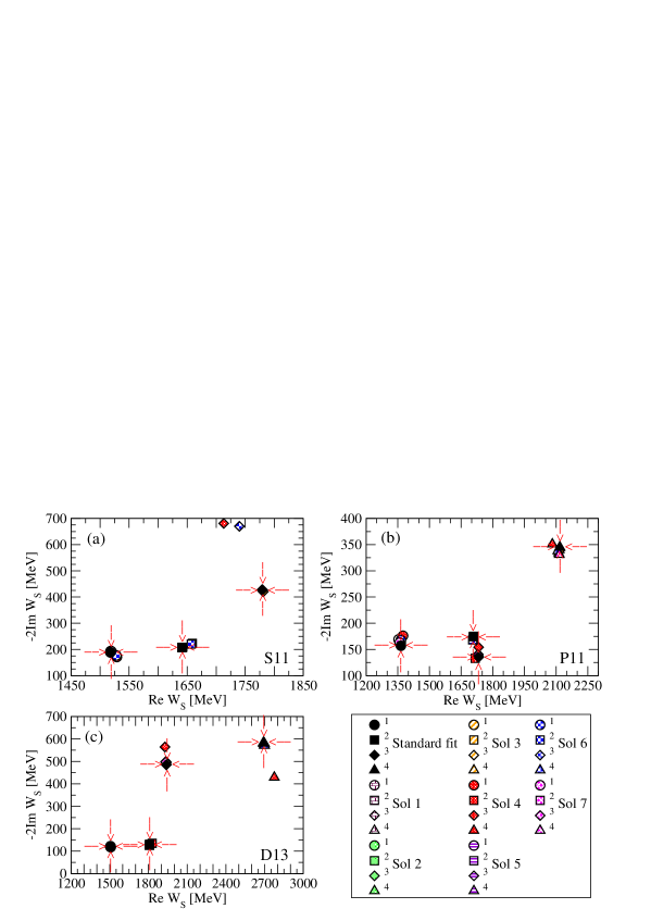
Figure 13: (Color online) The extracted $S_{11}$, $P_{11}$ and $D_{13}$ partial waves T-matrix poles. Additional background poles below and above physical region are added. Red arrows indicate the position of Standard solution poles.

Conclusion:

In Tables 14- 16 in Fig. (13) we see that all extracted bare and dressed poles are practically identical with the exception of solutions $Sol\ 4$ and $Sol\ 6$. And these are solutions where only 1 subthreshold pole has been allowed.

Therefore:

1. at least two background poles are needed to adequately represent the energy dependent background.

2. two subthreshold poles are enough to adequately represent the background. Two pole meromorphic approximation for the background representation is justified.

V.5 Number of channels

It is not self evident that introducing new channels, i.e. new contributions to the self energy term in the denominator of Eq. (11), does not influence pole positions at all. Namely, self energy matrix is of higher order, and self energy is distributed in a different way. To test this assumption we have introduced the fourth channel, and fitted the existing data base with this channel.

In addition to the existing $\pi$N elastic and $\pi\!N\!\rightarrow\!\eta N\>$ processes we have introduced a third channel opening at 1612 MeV (K$\Lambda$ channel). The mass of the effective channel has not been altered, as the effective channel is primarily dominated by the $\pi\pi$N channel. The results are given in Tables 17 - 19.

Table 17: Extracted $S_{11}$ partial wave T-matrix poles obtained by including three and four channels into a model.

	Bare poles			Dressed poles
Solutions	$\mathrm{W_{s_{1}}}$	$\mathrm{W_{s_{2}}}$	$\mathrm{W_{s_{3}}}$	$\begin{pmatrix}\mathrm{ReW}\\ \mathrm{-2ImW}\end{pmatrix}$	$\begin{pmatrix}\mathrm{ReW}\\ \mathrm{-2ImW}\end{pmatrix}$	$\begin{pmatrix}\mathrm{ReW}\\ \mathrm{-2ImW}\end{pmatrix}$	$\mathrm{\chi_{R}^{2}}$
		$\mathrm{MeV}$			$\mathrm{MeV}$
Sol 3CH	1523	1640	1834	$\begin{pmatrix}1518\\ 189\end{pmatrix}$	$\begin{pmatrix}1642\\ 208\end{pmatrix}$	$\begin{pmatrix}1779\\ 427\end{pmatrix}$	1.016
Sol 4CH	1523	1640	1836	$\begin{pmatrix}1516\\ 190\end{pmatrix}$	$\begin{pmatrix}1642\\ 211\end{pmatrix}$	$\begin{pmatrix}1776\\ 418\end{pmatrix}$	1.013

Table 18: Extracted $P_{11}$ partial wave T-matrix poles obtained by including three and four channels into a model.

	Bare poles				Dressed poles
Solutions	$\mathrm{W_{s_{1}}}$	$\mathrm{W_{s_{2}}}$	$\mathrm{W_{s_{3}}}$	$\mathrm{W_{s_{4}}}$	$\begin{pmatrix}\mathrm{ReW}\\ \mathrm{-2ImW}\end{pmatrix}$	$\begin{pmatrix}\mathrm{ReW}\\ \mathrm{-2ImW}\end{pmatrix}$	$\begin{pmatrix}\mathrm{ReW}\\ \mathrm{-2ImW}\end{pmatrix}$	$\begin{pmatrix}\mathrm{ReW}\\ \mathrm{-2ImW}\end{pmatrix}$	$\mathrm{\chi_{R}^{2}}$
		$\mathrm{MeV}$				$\mathrm{MeV}$
Sol 3CH	1607	1772	2182	2841	$\begin{pmatrix}1365\\ 157\end{pmatrix}$	$\begin{pmatrix}1708\\ 174\end{pmatrix}$	$\begin{pmatrix}1731\\ 136\end{pmatrix}$	$\begin{pmatrix}2117\\ 345\end{pmatrix}$	0.958
Sol 4CH	1607	1772	2182	2841	$\begin{pmatrix}1363\\ 161\end{pmatrix}$	$\begin{pmatrix}1708\\ 174\end{pmatrix}$	$\begin{pmatrix}1731\\ 136\end{pmatrix}$	$\begin{pmatrix}2117\\ 343\end{pmatrix}$	0.970

Table 19: Extracted $D_{13}$ partial wave T-matrix poles obtained by including three and four channels into a model.

	Bare poles			Dressed poles
Solutions	$\mathrm{W_{s_{1}}}$	$\mathrm{W_{s_{2}}}$	$\mathrm{W_{s_{3}}}$	$\begin{pmatrix}\mathrm{ReW}\\ \mathrm{-2ImW}\end{pmatrix}$	$\begin{pmatrix}\mathrm{ReW}\\ \mathrm{-2ImW}\end{pmatrix}$	$\begin{pmatrix}\mathrm{ReW}\\ \mathrm{-2ImW}\end{pmatrix}$	$\begin{pmatrix}\mathrm{ReW}\\ \mathrm{-2ImW}\end{pmatrix}$	$\mathrm{\chi_{R}^{2}}$
		$\mathrm{MeV}$			$\mathrm{MeV}$
Sol 3CH	1582	1880	2499	$\begin{pmatrix}1506\\ 121\end{pmatrix}$	$\begin{pmatrix}1807\\ 127\end{pmatrix}$	$\begin{pmatrix}1939\\ 485\end{pmatrix}$	$\begin{pmatrix}2691\\ 583\end{pmatrix}$	1.027
Sol 4CH	1581	1890	2499	$\begin{pmatrix}1500\\ 169\end{pmatrix}$	$\begin{pmatrix}1808\\ 131\end{pmatrix}$	$\begin{pmatrix}1944\\ 492\end{pmatrix}$	$\begin{pmatrix}2689\\ 586\end{pmatrix}$	1.035

Conclusion:

Pole position for the analyzed partial waves are extremely stable with respect to the opening of a new channel.

V.6 Mass of the effective channel

However, in spite of looking identical to all other tests, choice of the effective cannel mass undergoes strong physical constraints:

1. The effective channel represents all inelastic two and three body channels as only one, stable, two body channel. This is a serious assumption because some channels, the dominant three body channel like $\pi\pi N$ and unstable ones like $\sigma N$ and $\rho N$ introduce a significantly different analytic structure, so this might influence the conclusion on existence of some resonant states. An indication that it might be actually happening is already given for the $\rho N$ channel where its complex branchpoint for the P₁₁ partial wave lies dangerously close to the P₁₁(1710) resonance - see ref. Ceci2011 . Genuine three body effects for the dominant $\pi\pi N$ channel might also cause serious problem, This particularities should be analyzed as they are detected, but the method in general can enable statistical analyses of most of other resonant states.

2. As the effective channel represents the loss of flux to all inelastic channels, its mass has to be neither to high nor too low. If it is too high, the loss of flux to inelastic channels imposed by the data at energies below effective channel threshold will not be compensated by the third channel, so the T-matrix values will simply be too high to fit the data. If the mass is too low, we shall artificially open the new degrees of freedom where they actually do not exist. So, the mass of the effective channel will be fairly precisely defined by all inelastic channels.

3. When the effective channel mass is changed, the effective channel T-matrix threshold is also shifted. Therefore, the code will unsuccessfully try to reproduce the inelastic channel data which are generated by the different threshold, and move other resonances.

Therefore, we have decided to show both aspects of the problem for the $S_{11}$, $P_{11}$ and $D_{13}$ partial waves: In Fig (14) and Tables 20 - 22 we illustrate what is happening to the poles when the mass of the effective channel is changed $\pm$ 40%.

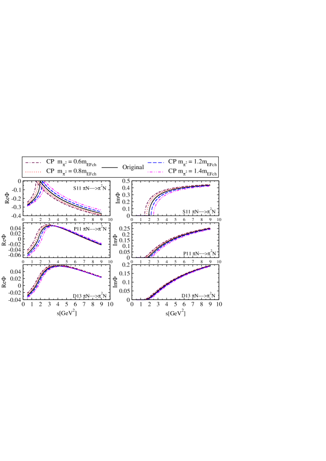
Figure 14: (Color online) Real and imaginary parts of $S_{11}$, $P_{11}$ and $D_{13}$ effective channel propagator.

Result:

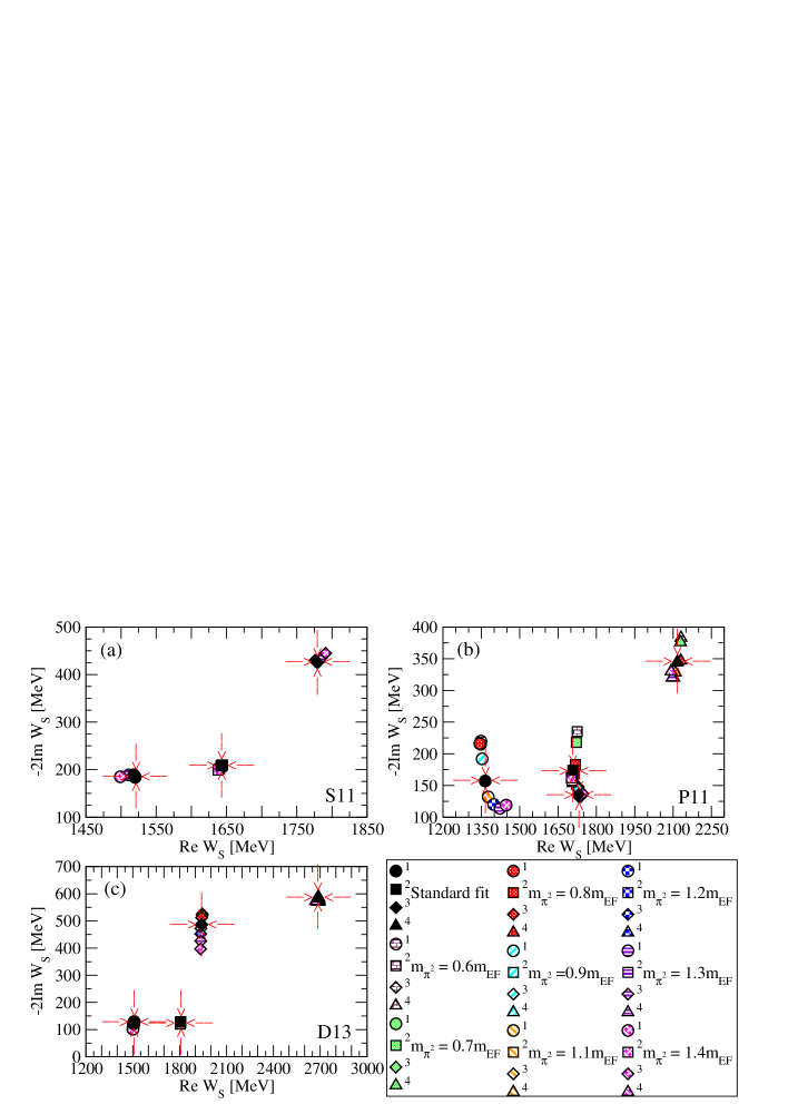
Figure 15: (Color online) The extracted $S_{11}$, $P_{11}$ and $D_{13}$ partial waves T-matrix poles using different mass of the effective channel.

The shift in pole positions for partial waves S₁₁, P₁₁ and D₁₃ are presented in Tables 20- 22 and depicted in Fig. (15).

Table 20: The extracted $S_{11}$ partial wave T-matrix poles using different mass of effective channel

	Bare poles			Dressed poles
Solutions	$\mathrm{W_{s_{1}}}$	$\mathrm{W_{s_{2}}}$	$\mathrm{W_{s_{3}}}$	$\begin{pmatrix}\mathrm{ReW}\\ \mathrm{-2ImW}\end{pmatrix}$	$\begin{pmatrix}\mathrm{ReW}\\ \mathrm{-2ImW}\end{pmatrix}$	$\begin{pmatrix}\mathrm{ReW}\\ \mathrm{-2ImW}\end{pmatrix}$	$\mathrm{\chi_{R}^{2}}$
		$\mathrm{MeV}$			$\mathrm{MeV}$
Sol $0.6m_{EF}$	1522	1637	1823	$\begin{pmatrix}1520\\ 184\end{pmatrix}$	$\begin{pmatrix}1644\\ 210\end{pmatrix}$	$\begin{pmatrix}1776\\ 430\end{pmatrix}$	1.028
Sol $0.7m_{EF}$	1523	1638	1825	$\begin{pmatrix}1520\\ 184\end{pmatrix}$	$\begin{pmatrix}1644\\ 209\end{pmatrix}$	$\begin{pmatrix}1777\\ 430\end{pmatrix}$	1.024
Sol $0.8m_{EF}$	1523	1638	1827	$\begin{pmatrix}1520\\ 185\end{pmatrix}$	$\begin{pmatrix}1644\\ 210\end{pmatrix}$	$\begin{pmatrix}1776\\ 429\end{pmatrix}$	1.020
Sol $0.9m_{EF}$	1523	1639	1830	$\begin{pmatrix}1519\\ 186\end{pmatrix}$	$\begin{pmatrix}1643\\ 209\end{pmatrix}$	$\begin{pmatrix}1779\\ 426\end{pmatrix}$	1.014
Standard fit	1523	1640	1834	$\begin{pmatrix}1518\\ 189\end{pmatrix}$	$\begin{pmatrix}1642\\ 208\end{pmatrix}$	$\begin{pmatrix}1779\\ 427\end{pmatrix}$	1.016
Sol $1.1m_{EF}$	1524	1641	1837	$\begin{pmatrix}1518\\ 188\end{pmatrix}$	$\begin{pmatrix}1642\\ 207\end{pmatrix}$	$\begin{pmatrix}1778\\ 427\end{pmatrix}$	1.003
Sol $1.2m_{EF}$	1524	1643	1842	$\begin{pmatrix}1516\\ 188\end{pmatrix}$	$\begin{pmatrix}1642\\ 206\end{pmatrix}$	$\begin{pmatrix}1781\\ 427\end{pmatrix}$	1.016
Sol $1.3m_{EF}$	1523	1643	1846	$\begin{pmatrix}1511\\ 189\end{pmatrix}$	$\begin{pmatrix}1640\\ 202\end{pmatrix}$	$\begin{pmatrix}1786\\ 437\end{pmatrix}$	1.062
Sol $1.4m_{EF}$	1522	1644	1850	$\begin{pmatrix}1499\\ 185\end{pmatrix}$	$\begin{pmatrix}1638\\ 199\end{pmatrix}$	$\begin{pmatrix}1791\\ 445\end{pmatrix}$	1.172

Table 21: The extracted $P_{11}$ partial wave T-matrix poles using different mass of the effective channel.

	Bare poles				Dressed poles
Solutions	$\mathrm{W_{s_{1}}}$	$\mathrm{W_{s_{2}}}$	$\mathrm{W_{s_{3}}}$	$\mathrm{W_{s_{4}}}$	$\begin{pmatrix}\mathrm{ReW}\\ \mathrm{-2ImW}\end{pmatrix}$	$\begin{pmatrix}\mathrm{ReW}\\ \mathrm{-2ImW}\end{pmatrix}$	$\begin{pmatrix}\mathrm{ReW}\\ \mathrm{-2ImW}\end{pmatrix}$	$\begin{pmatrix}\mathrm{ReW}\\ \mathrm{-2ImW}\end{pmatrix}$	$\chi_{R}^{2}$
		$\mathrm{MeV}$				$\mathrm{MeV}$
Sol $0.6m_{EF}$	1574	1775	2204	2826	$\begin{pmatrix}1348\\ 220\end{pmatrix}$	$\begin{pmatrix}1725\\ 235\end{pmatrix}$	$\begin{pmatrix}1729\\ 148\end{pmatrix}$	$\begin{pmatrix}2131\\ 383\end{pmatrix}$	1.827
Sol $0.7m_{EF}$	1582	1774	2199	2811	$\begin{pmatrix}1347\\ 215\end{pmatrix}$	$\begin{pmatrix}1722\\ 218\end{pmatrix}$	$\begin{pmatrix}1728\\ 144\end{pmatrix}$	$\begin{pmatrix}2129\\ 376\end{pmatrix}$	1.587
Sol $0.8m_{EF}$	1595	1772	2182	2773	$\begin{pmatrix}1344\\ 216\end{pmatrix}$	$\begin{pmatrix}1718\\ 183\end{pmatrix}$	$\begin{pmatrix}1725\\ 145\end{pmatrix}$	$\begin{pmatrix}2130\\ 347\end{pmatrix}$	1.272
Sol $0.9m_{EF}$	1600	1772	2178	2799	$\begin{pmatrix}1353\\ 192\end{pmatrix}$	$\begin{pmatrix}1714\\ 169\end{pmatrix}$	$\begin{pmatrix}1729\\ 145\end{pmatrix}$	$\begin{pmatrix}2115\\ 344\end{pmatrix}$	1.002
Standard fit	1607	1772	2182	2841	$\begin{pmatrix}1365\\ 157\end{pmatrix}$	$\begin{pmatrix}1708\\ 174\end{pmatrix}$	$\begin{pmatrix}1731\\ 136\end{pmatrix}$	$\begin{pmatrix}2117\\ 345\end{pmatrix}$	0.958
Sol $1.1m_{EF}$	1614	1773	2184	2811	$\begin{pmatrix}1377\\ 132\end{pmatrix}$	$\begin{pmatrix}1707\\ 163\end{pmatrix}$	$\begin{pmatrix}1732\\ 132\end{pmatrix}$	$\begin{pmatrix}2109\\ 328\end{pmatrix}$	1.182
Sol $1.2m_{EF}$	1615	1775	2182	2809	$\begin{pmatrix}1399\\ 120\end{pmatrix}$	$\begin{pmatrix}1705\\ 156\end{pmatrix}$	$\begin{pmatrix}1735\\ 132\end{pmatrix}$	$\begin{pmatrix}2103\\ 320\end{pmatrix}$	2.215
Sol $1.3m_{EF}$	1608	1777	2175	2832	$\begin{pmatrix}1423\\ 114\end{pmatrix}$	$\begin{pmatrix}1704\\ 158\end{pmatrix}$	$\begin{pmatrix}1735\\ 132\end{pmatrix}$	$\begin{pmatrix}2103\\ 320\end{pmatrix}$	4.166
Sol $1.4m_{EF}$	1592	1779	2166	2883	$\begin{pmatrix}1447\\ 119\end{pmatrix}$	$\begin{pmatrix}1702\\ 162\end{pmatrix}$	$\begin{pmatrix}1747\\ 137\end{pmatrix}$	$\begin{pmatrix}2092\\ 330\end{pmatrix}$	7.021

Table 22: The extracted $D_{13}$ partial wave T-matrix poles using different mass of the effective channel

	Bare poles			Dressed poles
Solutions	$\mathrm{W_{s_{1}}}$	$\mathrm{W_{s_{2}}}$	$\mathrm{W_{s_{3}}}$	$\begin{pmatrix}\mathrm{ReW}\\ \mathrm{-2ImW}\end{pmatrix}$	$\begin{pmatrix}\mathrm{ReW}\\ \mathrm{-2ImW}\end{pmatrix}$	$\begin{pmatrix}\mathrm{ReW}\\ \mathrm{-2ImW}\end{pmatrix}$	$\begin{pmatrix}\mathrm{ReW}\\ \mathrm{-2ImW}\end{pmatrix}$	$\mathrm{\chi_{R}^{2}}$
		$\mathrm{MeV}$			$\mathrm{MeV}$
Sol $0.6m_{EF}$	1580	1878	2496	$\begin{pmatrix}1509\\ 129\end{pmatrix}$	$\begin{pmatrix}1808\\ 129\end{pmatrix}$	$\begin{pmatrix}1945\\ 526\end{pmatrix}$	$\begin{pmatrix}2687\\ 588\end{pmatrix}$	1.096
Sol $0.7m_{EF}$	1580	1878	2496	$\begin{pmatrix}1508\\ 129\end{pmatrix}$	$\begin{pmatrix}1808\\ 128\end{pmatrix}$	$\begin{pmatrix}1944\\ 520\end{pmatrix}$	$\begin{pmatrix}2687\\ 589\end{pmatrix}$	1.069
Sol $0.8m_{EF}$	1580	1879	2499	$\begin{pmatrix}1507\\ 127\end{pmatrix}$	$\begin{pmatrix}1807\\ 128\end{pmatrix}$	$\begin{pmatrix}1941\\ 512\end{pmatrix}$	$\begin{pmatrix}2688\\ 589\end{pmatrix}$	1.041
Sol $0.9m_{EF}$	1582	1880	2499	$\begin{pmatrix}1507\\ 124\end{pmatrix}$	$\begin{pmatrix}1807\\ 127\end{pmatrix}$	$\begin{pmatrix}1940\\ 488\end{pmatrix}$	$\begin{pmatrix}2691\\ 578\end{pmatrix}$	1.044
Standard fit	1582	1880	2499	$\begin{pmatrix}1506\\ 121\end{pmatrix}$	$\begin{pmatrix}1807\\ 127\end{pmatrix}$	$\begin{pmatrix}1939\\ 485\end{pmatrix}$	$\begin{pmatrix}2691\\ 583\end{pmatrix}$	1.027
Sol $1.1m_{EF}$	1583	1880	2499	$\begin{pmatrix}1505\\ 118\end{pmatrix}$	$\begin{pmatrix}1807\\ 127\end{pmatrix}$	$\begin{pmatrix}1936\\ 472\end{pmatrix}$	$\begin{pmatrix}2694\\ 572\end{pmatrix}$	0.996
Sol $1.2m_{EF}$	1584	1881	2501	$\begin{pmatrix}1503\\ 113\end{pmatrix}$	$\begin{pmatrix}1806\\ 126\end{pmatrix}$	$\begin{pmatrix}1935\\ 452\end{pmatrix}$	$\begin{pmatrix}2690\\ 570\end{pmatrix}$	1.031
Sol $1.3m_{EF}$	1586	1882	2504	$\begin{pmatrix}1502\\ 108\end{pmatrix}$	$\begin{pmatrix}1805\\ 123\end{pmatrix}$	$\begin{pmatrix}1935\\ 426\end{pmatrix}$	$\begin{pmatrix}2681\\ 571\end{pmatrix}$	1.127
Sol $1.4m_{EF}$	1589	1883	2507	$\begin{pmatrix}1501\\ 101\end{pmatrix}$	$\begin{pmatrix}1804\\ 120\end{pmatrix}$	$\begin{pmatrix}1934\\ 397\end{pmatrix}$	$\begin{pmatrix}2670\\ 573\end{pmatrix}$	1.325

Conclusion:

We see that increasing the mass of the effective channel too much above the threshold of the first inelastic channel contributing to the particular partial wave is producing unrealistic shifts of the pole positions.

Reducing the mass for up to 40% is producing some shift, but not significant. And again we see that the T-matrix poles form two classes: the first class–almost stable poles S₁₁ (1518), S₁₁ (1642), D₁₃ (1506), D₁₃ (1807), and D₁₃ (2691) and the second class– more sensitive poles S₁₁ (1779), P₁₁ (1506), P₁₁ (1708), P₁₁ (1731), P₁₁ (2117), and D₁₃ (1939). The pole is not sensitive to the model parameters if it is dominantly determined by the bare singularity (small self energy correction), and it is moderately or strongly sensitive upon the model choices if the pole is created more dynamically (self energy contribution is strong).

From Tables 20-22 it is seen that reduced $\chi^{2}$ significantly raises when we increase the mass of the effective channel for up to 40%. This is, however, not so when the mass of effective channel is decreased for the same amount. We can easily understand the effect. Namely, the effective channel serves for ensuring unitarity for all open inelastic channels. However, if we increase the mass of the inelastic channel too much, then the fit, which is manifestly unitary, will not have an extra channel at its disposal to get rid of unwanted flux, and the code will be forced to fit the input data with amplitudes which are much more “elastic” then in reality. Simply, there will be no room for the loss of flux to inelastic channels which are open at these energies. Therefore, the fit will produce unrealistic results. On the other hand, if we lower the mass of the effective channel for 40%, we shall allow the fit to send the flux to inelastic channel if needed. However, the fit declines this possibility because the input data are dominantly elastic.

VI Conclusions

In our model we find two classes of poles: ones strongly determined by the bare poles, and ones which are more influenced by the self energy correction.

Poles S₁₁ (1518), S₁₁ (1642), P₁₁ (1731), D₁₃ (1506) and D₁₃ (1807) belong to the first class, and S₁₁ (1779), $P_{11}(1365)$, P₁₁ (1708), P₁₁ (2117), D₁₃ (1939) and D₁₃ (2691) to the second.

We show that the position of bare poles is model dependent. It is strongly influenced by dispersion relation subtraction constant and the channel propagator threshold behavior. As we believe that the threshold behavior is fairly well determined by the $q^{2L+1}$ law, the major model freedom of bare poles is originating from the choice of dispersion relation subtraction constant.

The dressed pole positions are much better fixed. Poles for which the self energy correction is small are stable, and ones for which the self energy correction is stronger are only moderately running. The “complex plane distance” between bare and dressed poles representing the size of the self energy contributions can be taken as a measure how model dependent a certain pole is. The smaller the difference is, the more confident the pole extraction is.

We observe that the reduced $\chi^{2}_{R}$, the quantity representing the measure of ability of our model to reproduce the input data, is systematically smallest for the non-modified solution. In other words, our model is unable to correctly fit the input data whenever any significant change to the model ingredients is introduced. We conclude that our model is sensitive to the analytic structure embedded into the input data by the way they are generated, because the underlying analytical structure of the Zagreb model is transferred to the data when we created the input data set by distributing Zagreb theoretical curves. If our analytic structure is wrong, and it certainly has to be up to a certain level, the real data coming from the experiment are described by the different analytic function and will not be ideally fitted by our curves. So, pole positions will be shifted.

However, we could at least in principle, use this feature as to test the shape of the model ingredients determining the self energy corrections. We propose the following procedure to improve the analytic structure of Zagreb CMB model with respect to any input data, either originating from different PWA or preferably coming directly from experiment in the form of partial wave data:

1. We fit the obtained input set and get the pole positions with the standard channel propagator, and note the belonging $\chi^{2}_{R}$.

2. We change the form of the channel propagator, re do the fit, and compare the new $\chi^{2}_{R}$ with the old value.

3. If the $\chi^{2}_{R}$ is better, we keep on changing the form of the channel propagator because we infer that our imposed analytic structure is not adequate, and that we are finding the better one.

4. When we achieve the best $\chi^{2}_{R}$, we pronounce that we have found the optimal value of the channel propagator for our formalism, and declare the found pole positions a correct ones.

5. We should, in principle, be able to follow which poles are changed, and which remain stable, and on the basis of that infer the error.

However, the afore hinted procedure is not within the scope of this paper.

In conclusion:

Zagreb CMB model can be used for extracting dressed pole positions from either partial wave data or partial wave amplitudes. The bare pole masses are strongly model dependent, while the dressed pole positions are much better fixed. The poles which are strongly influenced by the self energy corrections, however, show more model dependence then the ones which are dominated by the bare poles. At this point it is important to mention that our findings about the relative size of bare vs. self energy contributions of a certain pole are not eternal truth for all models. As bare mass is a movable quantity, it is easy to imagine that for some other model the shift of the bare pole position in proper direction might result in reducing the importance of self energy corrections. So, poles which are dominated by self energy corrections in our model might be dominated by the bare pole in others. This allows us to speculate that changing the subtraction constant that is a completely free parameter of our model may shift the results of Zagreb CMB fit in the direction of other models with respect to the value of bare poles.

There are other interesting questions like the role of physical requirements on the S-matrix that are missing in the Zagreb CMB model. Those are, e.g., sub-threshold cuts (circular, short nucleon, left-hand cuts as we have a trivial left-hand cut from kinematics, but that is, of course, not the full one…), or true and not effective three-body intermediate states with the corresponding additional analytic structures in the complex plane. Those are the really questions of exceptional interest which are really hard to answer, and will not be answered yet in this paper.

References

- (1) M. Hadžimehmedović, S. Ceci, A. Švarc, H. Osmanović, and J. Stahov, arXiv:1103.2653, submitted for publication to Phys. Rev. C.
- (2) G. Höhler, in Pion-Nucleon Scattering, Landolt-Börnstein, Vol I/9b2 (Springer-Verlag, Berlin, 1983); G. Höhler and A. Schulte, Newsletter, 7 (1992) 407.
- (3) http://gwdac.phys.gwu.edu/analysis/pin_analysis.html.
- (4) R. A. Arndt, W.J. Briscoe, I.I. Strakovsky, R.L. Workman, and M.M. Pavan, Phys. Rev. C69, 035213 (2004), R. A. Arndt, W. J. Briscoe, I. I. Strakovsky, and R. L. Workman, Phys. Rev. C 74, 045205 (2006).
- (5) B. Juliá - Díaz, T.-S. H. Lee, A. Matsuyama, and T. Sato, Phys. Rev. C 76, 065201 (2007).
- (6) J. Durand, B. Juliá - Díaz, T.-S. H. Lee, B. Saghai, and T. Sato, Rev. C 78, 025204 (2008).
- (7) A. Matsuyama, T. Sato, and T.-S.H. Lee, Physics Reports 439, 193 (2007).
- (8) M. Döring, C. Hanhart,, F. Huang, S. Krewald, and U.-G. Meissner, Nucl.Phys, A 829, 170 (2009); C. Schütz, J. Haidenbauer, J. Speth, and J. W. Durso, Phys. Rev. C 57 1464 (1998); O. Krehl, C. Hanhart, S. Krewald, and J. Speth, Phys. Rev. C 62 025207 (2000); A. M. Gasparyan, J. Haidenbauer, C. Hanhart, and J. Speth, Phys. Rev. C 68 045207 (2003).
- (9) Guan-Yeu Chen, S.S. Kamalov, Shin Nan Yang, D. Drechsel, and L. Tiator, Nuclear Physics A 723, 447 (2003).
- (10) Guan Yeu Chen, S. S. Kamalov, Shin Nan Yang, D. Drechsel and L. Tiator, Phys. Rev. C76, 035206 (2007).
- (11) V. Shklyar, H. Lenske, and U. Mosel, Phys. Rev. C 72, 015210 (2005), and private communication.
- (12) R. E. Cutkosky, C.P. Forsyth, R.E. Hendrick, and R.L. Kelly, Phys. Rev. D 20, 2839 (1979).
- (13) T. P. Vrana, S. A. Dytman, T. -S. H. Lee, Phys. Rep. 328,181 (2000).
-
(14)
A.V. Anisovich, A.V. Sarantsev, Eur.Phys.J. A30 , 427 (2006), and
http://pwa.hiskp.uni-bonn.de/. - (15) G. Höhler, in NSTAR2001, Proceedings of the Workshop on The Physics of Excited Nucleons, ed. D. Drechsel and L. Tiator, World Scientific 2001, 185.
- (16) G.F. Chew, Resonances, Particles, and Poles from the Experimenter s Point of View. Berkeley UCRL-16983 (1966).
- (17) G. Höhler in D.E. Groom et al., Particle Data Group, Eur. Phys. Jour. C 15, 1 (2000).
- (18) W. N. Cottingham, D. A. Greenwood, “An Introduction to Nuclear Physics”, Cambridge University Press, Cambridge 1986 and 2001.
- (19) R. H. Dalitz and R. G. Moorhouse, What is Resonance? Proc. R. Soc. Lond. A 318, 279-298 (1970).
- (20) R. H. Dalitz, Ann. Rev. Nucl. Science 13, 471 (1961).
- (21) J. von Neumann and E. P. Wigner, Z. Physik 30, 467 (1929).
- (22) M. Batinić, I. Šlaus, A. Švarc, and B.M.K. Nefkens, Phys. Rev. C 51, 2310 (1995); M. Batinić, I. Dadić, I. Šlaus, A. Švarc, B.M.K. Nefkens, and T.-S.H. Lee, Physica Scripta 58, 15, (1998).
- (23) M. Batinić, S. Ceci, A. Švarc, and B. Zauner, Phys. Rev. C 82, 038203 (2010).
- (24) S. Ceci, M. Döring, C. Hanhart, S. Krewald, U.-G. Meissner, A. Švarc, Phys. Rev. C84, 015205 (2011).
- (25) E. Pietarinen, Nuovo Cimento Soc. Ital. Fis. 12A, 522 (1972).
- (26) I. Ciulli, S. Ciulli, and J. Fisher, Il Nuovo Cimento 23, 1129 (1962).
- (27) S. Ceci, A. Švarc, and B. Zauner, Phys. Rev. Lett. 97, 062002 (2006).
- (28) P.M. Morse and H. Fesbach, Methods of Theoretical Physics, McGraW- Hill, New York, 1953.
- (29) S. Capstick, A. Švarc, L. Tiator, J. Gegelia, M.M. Giannini, E. Santopinto, C. Hanhart, S. Scherer, T.-S.H. Lee, T. Sato and N. Suzuki, Eur. Phys. J. A 35, 253 (2008), and references therein.