Extreme value analysis of actuarial risks:
estimation and model validation

Abstract

We give an overview of several aspects arising in the statistical analysis of extreme risks with actuarial applications in view. In particular it is demonstrated that empirical process theory is a very powerful tool, both for the asymptotic analysis of extreme value estimators and to devise tools for the validation of the underlying model assumptions. While the focus of the paper is on univariate tail risk analysis, the basic ideas of the analysis of the extremal dependence between different risks are also outlined. Here we emphasize some of the limitations of classical multivariate extreme value theory and sketch how a different model proposed by Ledford and Tawn can help to avoid pitfalls. Finally, these theoretical results are used to analyze a data set of large claim sizes from health insurance.

1 Introduction

In nonlife insurance, usually extreme events constitute a considerable portion of the total risk covered by an insurance company. Therefore, in actuarial practice extreme value statistics (though often in a simplified form) has been used for at least two decades to assess the risk of large claims. Given their exposure to huge claims, it is natural that reinsurers were among the first to emphasize the need for appropriate models of losses exceeding high thresholds. While the use of Pareto distributions and generalizations thereof were advocated early (see, e.g., Schmutz and Doerr (1998)), the fact that they naturally arise as approximative models for exceedances was not always fully acknowledged, but they were often considered yet another useful parametric model.

This situation has thoroughly changed. Nowadays it is rarely called into question that the assessment of “tail risks” requires specific methods and that extreme value theory often (though not always) offers efficient and mathematically sound procedures to deal with such problems. Moreover, several smooth introductions both to general extreme value statistics and to its application to actuarial problems have been published; see, e.g., Embrechts et al. (1997), Beirlant et al. (2004), McNeil (1997) and Cebrián et al. (2003). For that reason, the present paper focusses on specific aspects which have perhaps not attracted the attention they deserve:

• We will show that empirical process theory offers a general framework to deal with different steps in the risk analysis from model fitting to model validation and the estimation of risk measures.

• An important step in a prudent risk assessment is to validate the model assumptions on which the statistical analysis is based. To this end, graphical tools like qq-plots are widely used but the assessment which deviations from the ideal line indicate a violation of the model assumptions is largely subjective, and experience from classical statistical applications can be misleading if one analyzes heavy-tailed data. Hence in Section 4 it is described how to refine such tools to obtain a rigorous statistical test.

• The analysis of the dependence between different extreme risks has been extensively discussed in the recent statistical literature. We will first comment on problems arising when parametric copula models are used to this end. Then we discuss how to overcome a serious weakness of classical multivariate extreme value statistics.

As the choice of topics addressed by such a partial survey is subjective, it is inevitable that some readers will miss aspects they consider particularly important. Perhaps the most obvious topic we only touch on concerns the extreme value analysis of investment risks. Although recent years have shown that in some instances the asset side of the balance book contains the most serious risks of extreme losses, for several reasons here we will nevertheless focus on “genuine” actuarial problems related to the insured risks. Firstly, the statistical and economic literature on extreme investment risks is abound. Secondly, though the very basics of extreme value theory needed in this context is the same as the one discussed here, a serious treatment of market risks would require a lengthy introduction to the extreme value behavior of time series; we refrain from discussing this topic in detail in order not to overload the article. Finally, we feel that mathematically satisfactory solutions are yet to be developed for important practical problems like the risk assessment for complex portfolios. An exposition that cannot go into great details carries the risk of provoking a serious misconception of the solutions that the state of the art in statistical theory can actually deliver.

As there are plenty of other important problems we can merely touch on, we will try to mitigate this lack by giving references where aspects important in actuarial applications are discussed in greater detail. We do however not aim at giving a full overview over the rapidly expanding literature relevant in this context. Hence the present text may be best characterized as a tutorial with particular emphasis laid on crucial points which, from my personal point of view, have often not attracted the interest they deserve.

The paper is organized as follows. Section 2 gives an introduction into the basics of univariate extreme value theory, with particular emphasis on conditional distributions of exceedances (instead of the distribution of maxima as in the classical approach). In Section 3 we discuss how to construct extreme value estimators of quantities like risk measures and insurance premiums which depend only on the tail behavior. Then Section 4 deals with methods to define a tail region depending on the data and the purpose and methods of the tail analysis as well as tools for model validation. In both these sections, a limit theorem for the tail empirical quantile function proves extremely useful. In Section 5 we outline how the dependence structure between the components of a vector of risks can be statistically analyzed. In Section 6 the previously introduced statistical procedures are used to analyze a data set of large claims in US health insurances. All proofs are deferred to the final Section 7.

2 Basics of univariate extreme value theory

Classically a synopsis on extreme value theory starts with the analysis of maxima of independent and identically distributed random variables (iid rv’s). We prefer to discuss the asymptotic behavior of excesses over high thresholds, because these naturally arise as effective claim sizes in insurances with high retention levels, while the maximum of claim sizes rarely is an economically meaningful quantity.

In what follows, let $X$ denote a rv defined on some probability space $(\Omega,\mathcal{A},P)$ with cumulative distribution function (cdf) $F$ and quantile function ${F^{\leftarrow}}$ (i.e., the generalized inverse of $F$). If $X$ describes a loss covered by an insurance with retention level $u$, then

$$F_{u}(x):=P(X-u\leq x\mid X>u)$$

is the cdf of the actual claim size. For a very high retention level $u$ (e.g., in an excess of loss reinsurance against catastrophes), usually few or none of the losses observed so far exceed $u$, so that standard methods for risk modeling and premium calculation do not apply directly. Of course, one could assume a parametric model for all losses, estimate its parameters (provided the full losses are observed) and calculate the resulting conditional cdf of the excesses over $u$. Then, however, the fitted model for $F_{u}$ is largely determined by the bulk of losses that are much smaller than the losses of interest that exceed $u$. Hence such an approach seems advisable only if one is confident that the same “stochastic mechanism” generates the moderate losses on the one hand and large losses on the other hand, and that all these losses can be well described by the chosen parametric model. As this will rarely be justified, it is widely accepted that for modeling $F_{u}$ one should consult only losses which are large, though perhaps still smaller than $u$. Sometimes this general idea is subsumed in the catchy phrase “Let the tails speak for themselves”.

The basic idea of extreme value theory is to tackle this problem by assuming that, after a suitable normalization, the cdf $F_{u}$ converges to a non-degenerate limit as the threshold $u$ tends to the largest possible loss ${F^{\leftarrow}}(1)$. More precisely, we assume that for some (measurable) function $a>0$ there exists a non-degenerate cdf $H$ (i.e., $H(\mathbb{R})\not\subset\{0,1\}$) such that

$$F_{u}(a(u)x)=P\Big{(}\frac{X-u}{a(u)}\leq x\,\Big{|}\,X>u\Big{)}\to H(x)$$ (2.1)

as $u\uparrow{F^{\leftarrow}}(1)$ for all points of continuity $x$ of $H$ (i.e., $F_{u}(a(u)\cdot)\to H$ weakly). It turns out that then $H$ is necessarily the cdf of a generalized Pareto distribution (GPD), that is

$$H(x)=H_{\gamma,\sigma}(x)=\left\{\begin{array}[]{l@{\quad}c@{\quad}l}0&&x\leq 0,\\ 1-(1+\gamma x/\sigma)^{-1/\gamma}&\text{if}&x>0,1+\gamma x/\sigma>0,\\ 1&&1+\gamma x/\sigma\leq 0,\gamma<0.\end{array}\right.$$

Here $H_{0,\sigma}(x)$ is interpreted as $\lim_{\gamma\to 0}H_{\gamma,\sigma}(x)=(1-{\rm e}^{-x/\sigma})1_{[0,\infty)}(x)$, which is an exponential cdf. Note that the scale parameter depends on the choice of the normalizing function $a$; we can and will always assume $\sigma=1$ and write $H_{\gamma}$ instead of $H_{\gamma,1}$.

If (2.1) holds, then the conditional cdf $F_{u}$ can be approximated by $H_{\gamma,\sigma_{u}}$ with $\sigma_{u}=a(u)$, provided $u$ is sufficiently large. In that case, the following approximation of the tail of the loss cdf $F$ follows:

$$1-F(y)=(1-F(u))(1-F_{u}(y-u))\approx(1-F(u))\big{(}1-H_{\gamma,\sigma_{u}}(y-u)\big{)}$$ (2.2)

for $y\geq u$. Of course, this approximation can also be used for thresholds $u$ different from the retention level at hand. It is important to note that (almost) always (2.2) is only an approximation to the tail and that its accuracy depends on the choice of $u$. Hence one should avoid considering the GPD model to be the “true” one above a certain threshold $u$. As we will discuss in detail later on, there will always be a bias-variance trade-off when choosing a threshold to estimate premiums or risk measures.

The extreme value approach to the analysis of $F_{u}$ relies on convergence (2.1). Fortunately, almost all textbook distributions suggested to model claim sizes fulfill this condition, that can be reformulated as

$$\lim_{u\uparrow{F^{\leftarrow}}(1)}\frac{1-F(u+a(u)x)}{1-F(u)}=1-H_{\gamma}(x),\quad x>0,$$ (2.3)

for some $\gamma\in\mathbb{R}$. It is easily seen that this condition holds if and only if for $\tilde{a}(t)=a({F^{\leftarrow}}(1-t))$

$$\lim_{t\downarrow 0}\frac{{F^{\leftarrow}}(1-tx)-{F^{\leftarrow}}(1-t)}{\tilde{a}(t)}=H_{\gamma}^{\leftarrow}(1-x)=\frac{x^{-\gamma}-1}{\gamma},\quad x\in(0,1),$$ (2.4)

where the right-hand side is interpreted as $-\log x$ for $\gamma=0$. (Indeed, (2.4) holds for all $x>0$.)

The so-called extreme value index $\gamma$ largely determines the tail behavior of $F$. If $\gamma>0$, then the loss distribution is unbounded and (2.4) is equivalent to the regular variation of $1-F$ at $\infty$ and of ${F^{\leftarrow}}$ at 1:

$$\lim_{u\uparrow\infty}\frac{1-F(ux)}{1-F(u)} = x^{-1/\gamma},$$ (2.5)

$$\lim_{t\downarrow 0}\frac{{F^{\leftarrow}}(1-tx)}{{F^{\leftarrow}}(1-t)} = x^{-\gamma},\qquad x>0.$$ (2.6)

In this case, both $F$ and $X$ are called heavy-tailed. (Notice, however, that in the literature other meanings of the term “heavy-tailed distributions” are common, too.) Typical examples are Burr distributions, loggamma distributions and $t$ distributions. As the survival function $1-F(x)$ roughly decays as the power function $x^{-1/\gamma}$, large losses are the more likely the larger $\gamma$ is. In particular, the loss has infinite expectation if $\gamma>1$ and it has infinite variance if $\gamma\in(1/2,1)$.

If the extreme value index is negative, then the loss has bounded support, while for $\gamma=0$ the right endpoint of the loss distribution can be finite or infinite. For most textbook examples, including lognormal, gamma and normal distributions, the latter is true.

This article will mainly focus on the case $\gamma>0$, that is obviously the most troublesome from an insurer’s perspective. We will see that in the statistical analysis it is nevertheless sometimes better to work with the more general conditions (2.3) and (2.4) instead of the simpler conditions (2.5) and (2.6), that correspond to the particular choice $a(u)=\gamma u$.

We close this section with a brief outline of the relationship to the limit behavior of maxima of iid rv’s $X_{i}$, $1\leq i\leq n$, with cdf $F$. It can be shown that assumption (2.1) is equivalent to the convergence of the suitably standardized maxima to the (generalized) extreme value distribution corresponding to $H$, i.e.

$$\lim_{n\to\infty}P\Big{\{}\frac{\max_{1\leq i\leq n}X_{i}-b_{n}}{a_{n}}\leq x\Big{\}}=G(x)$$

holds for some $a_{n}>0$, $b_{n}\in\mathbb{R}$ and all points of continuity $x$ of the non-degenerate cdf $G$ if and only if (2.1) is fulfilled with $H=(1+\log G)^{+}$. Then it is said that $F$ belongs to the maximum domain of attraction ($F\in D(G)$ for short), and one can choose $b_{n}={F^{\leftarrow}}(1-1/n)$ and $a_{n}=a(b_{n})=\tilde{a}(1/n)$.

3 Univariate tail risk analysis

To start with a concrete problem, assume that based on observed losses $X_{1},\ldots,X_{n}$ the fair net premium of a (working) excess-of-loss (XL-) reinsurance with a cover of $c$ in excess of $t$ is to be estimated, that is, the reinsurer has to pay $\min((X-t)^{+},c)$ of all future claims $X$ exceeding $t$. After a suitable correction for inflation, the random variables $X_{i}$, $1\leq i\leq n$, shall be regarded as iid with some unknown cdf $F$. If at most a few observations exceed the retention level $t$, then the net premium per loss $E\big{(}\min((X-t)^{+},c)\big{)}$ cannot be directly estimated by the corresponding mean. Therefore, we assume that $F$ fulfills the basic condition (2.3) for some $\gamma\in\mathbb{R}$, so that we may approximate the net premium as follows:

$$E\big{(}\min((X-t)^{+},c)\big{)} = \int_{t}^{t+c}1-F(s)\,ds$$

$$= \int_{(t-u)/a(u)}^{(t+c-u)/a(u)}\frac{1-F(u+a(u)x)}{1-F(u)}\,dx\cdot a(u)(1-F(u))$$

$$\approx \int_{(t-u)/a(u)}^{(t+c-u)/a(u)}(1+\gamma x)^{-1/\gamma}\,dx\cdot a(u)(1-F(u))$$

$$= \bigg{[}\Big{(}1+\gamma\frac{t-u}{a(u)}\Big{)}^{1-1/\gamma}-\Big{(}1+\gamma\frac{t+c-u}{a(u)}\Big{)}^{1-1/\gamma}\bigg{]}\frac{a(u)(1-F(u))}{1-\gamma}$$

for some suitable threshold $u\leq t$, provided that $1+\gamma(t+c-u)/a(u)>0$. If $1-F(u)$ is sufficiently large, then it can be estimated by the corresponding empirical probability $1-F_{n}(u)$. Hence, if one replaces the extreme value $\gamma$ and the scale factor $a(u)$ by some estimators $\hat{\gamma}_{n}$ and $\hat{a}_{n}(u)$, respectively, then one obtains a reasonable estimator of the net premium per claim. (To obtain an estimator for the net premium of the whole XL reinsurance contract, one has to multiply this expression with some estimator of the expected number of claims.)

Estimators of $\gamma$ and $a(u)$ that use only exceedances over the threshold $u$ can be motivated in a similar way. For example, if one can assume that $\gamma$ is strictly positive, then by (2.5) the conditional distribution of $X/u$ given $X>u$ may be approximated by a Pareto distribution with Lebesgue density $\tilde{h}_{\gamma}(x)=x^{-(1/\gamma+1)}/\gamma$, $x>1$. Ignoring the approximation error and the fact that the number $N(u)$ of exceedances is also random, we may estimate $\gamma$ by a maximum likelihood approach to obtain

$$\hat{\gamma}_{n}:=\frac{1}{N(u)}\sum_{i=1}^{n}\log\frac{X_{i}}{u}1_{(u,\infty)}(X_{i}).$$ (3.2)

If one starts with condition (2.3) in the general case $\gamma\in\mathbb{R}$, then the conditional distribution of the excesses $X_{i}-u$ given $X_{i}>u$ are iid with approximative density $h_{\gamma}(x/\sigma)/\sigma=(1+\gamma x/\sigma)^{-(1/\gamma+1)}/\sigma$ for $1+\gamma x/\sigma>0$ with $\sigma:=a(u)$. As the resulting approximative likelihood is unbounded for $\gamma\leq-1$, a point of maximum of the loglikelihood $-(1/\gamma+1)\sum_{i=1}^{n}\log\big{(}1+\gamma(X_{i}-u)^{+}/\sigma\big{)}-N(u)\log\sigma$ on the parameter set $\{(\gamma,\sigma)\mid\gamma>-1,\sigma>-\gamma\max_{1\leq i\leq n}(X_{i}-u)^{+}\}$ can be motivated as an estimator for $(\gamma,a(u))$.

Of course, several other estimators of the extreme value index and the scale factor have been proposed; see, for instance, de Haan and Ferreira (2006), Sections 3 and 4.

The performance of all these estimators crucially depends on the accuracy of the (generalized) Pareto approximation in (2.3) (respectively (2.5) in the case $\gamma>0$) and the choice of the threshold $u$. Too low a threshold will lead to a large bias, because the GPD approximation is inaccurate for the smallest exceedances of $u$. On the other hand, if $u$ is chosen too large, then the estimators use only a very small fraction of the whole sample and thus their variance will be large. In Section 4, we will discuss methods to deal with the bias-variance tradeoff in greater detail.

Because one has to choose the threshold $u$ depending on the data, it seems natural to use a large order statistic $u=X_{n-k_{n}:n}$ (with $X_{i:n}$ denoting the $i$th smallest observation). Then all estimators under consideration are based on the $k_{n}+1$ largest observations and can therefore be written as functionals of the tail empirical quantile function

$$Q_{n}(t):=X_{n-[k_{n}t]:n},\quad t\in[0,1].$$ (3.3)

For example, replacing $u$ with $X_{n-k_{n}:n}$ in (3.2) yields the well-known Hill estimator

$$\hat{\gamma}_{n}:=\hat{\gamma}_{n,k_{n}}:=\frac{1}{k_{n}}\sum_{i=1}^{k_{n}}\log\frac{X_{n-i+1:n}}{X_{n-k_{n}:n}}$$ (3.4)

(if there are no ties).

Since the parameters $\gamma,a(u)$ and $\tilde{a}(t)$ are only defined by limit relations like (2.3) and (2.4), the performance of their estimators must be analyzed in an asymptotic framework. (Indeed, there are no unique “true” functions $a$ and $\tilde{a}$, because any function $\bar{a}$ such that $\bar{a}(t)/\tilde{a}(t)\to 1$ as $t\downarrow 0$ also satisfies (2.4).) Because the basic condition (2.4) describes the behavior of $F^{\leftarrow}$ only at its right endpoint $F^{\leftarrow}(1)$, in the asymptotic setting we must ensure that, while the number of order statistics used for the statistical tail analysis tends to infinity, all order statistics tend to $F^{\leftarrow}(1)$, that is, $(k_{n})_{n\in\mathbb{N}}$ is a so-called intermediate sequence satisfying

$$k_{n}\to\infty,\quad\frac{k_{n}}{n}\to 0.$$ (3.5)

Moreover, $k_{n}$ should not grow too fast to avoid the aforementioned bias problems due to a poor GPD approximation. The precise conditions on $k_{n}$ will be given below in terms of the approximation error in (2.4), i.e.

$$R(t,x):=\frac{{F^{\leftarrow}}(1-tx)-{F^{\leftarrow}}(1-t)}{\tilde{a}(t)}-\frac{x^{-\gamma}-1}{\gamma}.$$

As the randomness of all extreme value estimators under consideration is captured by the tail empirical quantile function, it is natural first to establish a limit theorem for this process and then to conclude the asymptotic behavior of quite general extreme value estimators (or tests) by a functional delta method. In what follows, we are focussing on the case $\gamma>-1/2$ and will often assume that $\gamma\geq 0$, which is by far the most relevant case in actuarial applications and helps to avoid technicalities. The following limit theorem (Drees, 1998a, Theorem 2.1) is the corner stone for the subsequent risk analysis

Theorem 3.1.

If $(k_{n})_{n\in\mathbb{N}}$ is an intermediate sequence such that for some $\tilde{\varepsilon}>0$

$$k_{n}^{1/2}\sup_{0<x\leq 1+\tilde{\varepsilon}}x^{\gamma+1/2}|R(k_{n}/n,x)|\;\to\;0,$$ (3.6)

then for a standard Brownian motion $W$ and all $\varepsilon>0$ we have

$$k_{n}^{1/2}\Big{(}\frac{Q_{n}(t)-{F^{\leftarrow}}(1-k_{n}/n)}{\tilde{a}(k_{n}/n)}-\frac{t^{-\gamma}-1}{\gamma}\Big{)}_{0<t\leq 1}\;\longrightarrow\;\big{(}t^{-(\gamma+1)}W(t)\big{)}_{0<t\leq 1}$$ (3.7)

weakly in the normed vector space $\big{(}D_{\gamma,\varepsilon},\|\cdot\|_{\gamma,\varepsilon}\big{)}$ of functions $z:(0,1]\to\mathbb{R}$ which are continuous from the right with left-hand limits and finite weighted supremum norm

$$\|z\|_{\gamma,\varepsilon}:=\sup_{0<t\leq 1}t^{\gamma+1/2+\varepsilon}\|z(t)\|.$$

It is noteworthy that, under the basic assumption (2.4), there always exist intermediate sequences $(k_{n})_{n\in\mathbb{N}}$ such that (3.6) is fulfilled. Hence (3.6) is not a condition on $F$, but it merely restricts the speed at which $k_{n}$ grows with the sample size.

Now suppose $T:D_{\gamma,\varepsilon}\to\mathbb{R}$ is a scale and shift invariant functional (i.e., $T(az+b)=T(z)$ for all $a>0$, $b\in\mathbb{R}$ and $z\in D_{\gamma,\varepsilon}$) such that $T(z_{\gamma})=\gamma$ for $z_{\gamma}(t):=(t^{-\gamma}-1)/\gamma$, such that the following (Hadamard) differentiability condition holds: there exists a signed measure $\nu_{T,\gamma}$ on $(0,1]$ such that

$$\frac{T(z_{\gamma}+\lambda_{n}y_{n})-T(z_{\gamma})}{\lambda_{n}}\;\longrightarrow\;\int y\,d\nu_{T,\gamma}$$ (3.8)

for all sequences $\lambda_{n}\downarrow 0$ and all $y_{n},y\in D_{\gamma,\varepsilon}$ satisfying $\|y_{n}-y\|_{\gamma,\varepsilon}\to 0$. Then one may easily deduce that

$$k_{n}^{1/2}\big{(}T(Q_{n})-\gamma\big{)}=k_{n}^{1/2}\Big{(}T\Big{(}\frac{Q_{n}-{F^{\leftarrow}}(1-k_{n}/n)}{\tilde{a}(k_{n}/n)}\Big{)}-\gamma\Big{)}\;\longrightarrow\;\int_{(0,1]}t^{-(\gamma+1)}W(t)\,\nu_{T,\gamma}(dt)\quad\text{weakly,}$$ (3.9)

where the right-hand side is normally distributed with expectation 0 and variance

$$\sigma_{T,\gamma}^{2}:=\int_{(0,1]}\int_{(0,1]}(st)^{-(\gamma+1)}\min(s,t)\,\nu_{T,\gamma}(ds)\,\nu_{T,\gamma}(dt).$$ (3.10)

Likewise, the scale factor $\tilde{a}(k_{n}/n)$ can be estimated by $S(Q_{n})$, where $S:D_{\gamma,\varepsilon}\to\mathbb{R}$ is a scale equivariant and shift invariant functional (i.e., $S(az+b)=aS(z)$ for all $a>0$, $b\in\mathbb{R}$ and $z\in D_{\gamma,\varepsilon}$) such that $S(z_{\gamma})=1$ and for some signed measure $\nu_{S,\gamma}$ on $(0,1]$

$$\frac{S(z_{\gamma}+\lambda_{n}y_{n})-S(z_{\gamma})}{\lambda_{n}}\;\longrightarrow\;\int y\,d\nu_{S,\gamma}$$ (3.11)

for all sequences $\lambda_{n}\downarrow 0$ and $\|y_{n}-y\|_{\gamma,\varepsilon}\to 0$. Then we conclude

$$k_{n}^{1/2}\Big{(}\frac{S(Q_{n})}{\tilde{a}(k_{n}/n)}-1\Big{)}\;\longrightarrow\;\int_{(0,1]}t^{-(\gamma+1)}W(t)\,\nu_{s,\gamma}(dt)\quad\text{weakly.}$$ (3.12)

(In fact, the joint weak convergence of (3.7), (3.9) and (3.12) holds.)

As an example, consider the functional $(T(z),S(z))$ defined as a solution $(\gamma,\sigma)$ of the equations

$$\int_{0}^{1}\frac{1}{1+\gamma(z(t)-z(1))/\sigma}\,dt = \frac{1}{\gamma+1}$$

$$\int_{0}^{1}\log\big{(}1+\gamma(z(t)-z(1))/\sigma\big{)}\,dt = \gamma$$

with $\gamma\neq 0$, or as $(0,\sigma)$ if $\big{(}\int_{0}^{1}z(t)-z(1)\,dt\big{)}^{2}=\int_{0}^{1}(z(t)-z(1))^{2}\,dt/2$ and $\sigma=\int_{0}^{1}z(t)-z(1)\,dt$. Then $(T(Q_{n}),S(Q_{n})$ is the aforementioned maximum likelihood estimator in the approximating GPD model (or more precisely, a solution of the corresponding likelihood equations). Using the methodology sketched above, one can prove that under the conditions of Theorem 3.1

$$k_{n}^{1/2}{T(Q_{n})-\gamma\choose S(Q_{n})/\tilde{a}(k_{n}/n)-1}\;\longrightarrow\;\mathcal{N}_{(0,\Sigma)}\quad\text{weakly with}\quad\Sigma:=\Big{(}\begin{array}[]{cc}(1+\gamma)^{2}&-(1+\gamma)\\ -(1+\gamma)&2+2\gamma+\gamma^{2}\end{array}\Big{)}.$$

It can be shown that these estimators have minimal asymptotic variances among all estimators $T(Q_{n})$ and $S(Q_{n})$ of the type discussed above. (See Drees (1998a) and Drees et al. (2004) for details.)

If $\gamma>0$, then one can always choose $\tilde{a}(t)=\gamma{F^{\leftarrow}}(1-t)$, so that (3.7) reads as

$$k_{n}^{1/2}\Big{(}\frac{Q_{n}(t)}{{F^{\leftarrow}}(1-k_{n}/n)}-t^{-\gamma}\Big{)}_{0<t\leq 1}\;\longrightarrow\big{(}\gamma t^{-(\gamma+1)}W(t)\big{)}_{0<t\leq t}\quad\text{weakly in }D_{\gamma,\varepsilon}.$$

Hence, in this case, we need not require that $T$ is shift invariant, but merely that it is scale invariant, which allows for a wider class of functionals. A prominent example is the Hill estimator $T_{H}(Q_{n})$ with $T_{H}(Z)=\int_{0}^{1}\log(z(t)/z(1))\,dt$, that is scale invariant but not shift invariant. The Hill estimator is asymptotically normal with asymptotic variance $\gamma^{2}$ if condition (3.6) is met for $\tilde{a}(t)=\gamma{F^{\leftarrow}}(1-t)$, which reads as

$$k_{n}^{1/2}\sup_{0<x\leq 1+\tilde{\varepsilon}}x^{\gamma+1/2}\Big{|}\frac{{F^{\leftarrow}}(1-k_{n}x/n)}{{F^{\leftarrow}}(1-k_{n}/n)}-x^{-\gamma}\Big{|}\;\longrightarrow\;0.$$ (3.13)

Note that for some cdf’s $F$ this condition imposes a much more severe restriction on the number of order statistics used for estimation than condition (3.6) for some other choice of the normalizing function $\tilde{a}$. Thus, even if it is known (or assumed) in advance that $\gamma>0$, it may be advisable to use the shift invariant ML estimator in the GPD model instead of the Hill estimator, although the latter has a smaller asymptotic variance.

Example 3.2.

Assume that the following expansion of the quantile function holds:

$${F^{\leftarrow}}(1-t)=d_{1}t^{-\gamma}+d_{2}+d_{3}t^{\rho-\gamma}+o(t^{\rho-\gamma})$$ (3.14)

for some $\gamma,\rho>0$, $d_{1}>0$ and $d_{2},d_{3}\neq 0$ with $d_{2}+d_{3}\neq 0$ if $\rho=\gamma$. Then condition (3.13) ensuring the asymptotic normality of the Hill estimator is equivalent to $k_{n}^{1/2}(k_{n}/n)^{\min(\gamma,\rho)}\to 0$ and hence to $k_{n}=o\big{(}n^{2\min(\gamma,\rho)/(2\min(\gamma,\rho)+1)}\big{)}$. In contrast, the ML estimator in the GPD model is asymptotically normal if condition (3.6) holds, e.g., with the choice $\tilde{a}(t)=\gamma d_{1}t^{-\gamma}$, which is equivalent to $k_{n}^{1/2}(k_{n}/n)^{\rho}\to 0$ and is hence fulfilled for $k_{n}=o(n^{2\rho/(2\rho+1)})$. For that reason, in the case $\rho>\gamma$, the ML estimator may use many more large order statistics than the Hill estimator before a significant bias shows up.

Remark 3.3.

It can be shown that, in the situation of Example 3.2, the shift invariant estimators $T(Q_{n})$ and $S(Q_{n})$ are still asymptotically normal if $k_{n}\sim\lambda n^{2\rho/(2\rho+1)}$ for some $\lambda>0$, but then the limiting normal distribution is no longer centered. See Drees (1998a) or de Haan and Ferreira (2006), Section 3, for similar results under second order refinements of condition (2.4), that are generalizations of expansion (3.14).

A different type of estimators for the extreme value index that explicitly uses these second order conditions are discussed in Section 4.5 of Beirlant et al. (2004). These estimators typically have a smaller bias in the more restrictive model, but their consistency is not ensured if only condition (2.3) or (2.5) is assumed.

Next we will demonstrate by the example of an estimator for the net premium of the XL-reinsurance discussed above that the asymptotic normality of a huge class of extreme value estimators follows by straightforward (though sometimes lengthy) computations. Replacing in (3) the threshold $u$ with $Q_{n}(1)=X_{n-k_{n}:n}$ and the unknown parameters by suitable estimators, we arrive at

$$\hat{\Pi}_{n}(t,c):=\frac{k_{n}}{n}S(Q_{n})\int_{(t-Q_{n}(1))/S(Q_{n})}^{(t+c-Q_{n}(1))/S(Q_{n})}(1+T(Q_{n})x)^{-1/T(Q_{n})}\,dx.$$

As explained above, we are interested in the case that at most a few observations exceed the retention level $t$. To reflect this crucial feature in the asymptotic framework, one must consider a sequence of retention levels $t=t_{n}$ which increases with the sample size. More precisely, we assume

$$\frac{n}{k_{n}}(1-F(t_{n}))\;\to\;0\quad\text{and}\quad\frac{1-F(t_{n}+c_{n})}{1-F(t_{n})}\;\to\;\lambda\in(0,1).$$ (3.15)

Despite the quite complex structure of the estimator $\hat{\Pi}_{n}(t_{n},c_{n})$, its asymptotic normality follows from the joint asymptotic normality of $T(Q_{n}),S(Q_{n})$ and $Q_{n}(1)$ by rather simple Taylor type expansions. For simplicity, we focus on the case $\gamma\geq 0$, but an analogous result can be proved by the same methodology for all $\gamma\in\mathbb{R}$. In the case $\gamma<0$, though, the asymptotic behavior of $\hat{\Pi}_{n}$ also depends on the asymptotics of $S(Q_{n})$, while it does not play a role in the following result.

Corollary 3.4.

Assume that $F\in D(G_{\gamma})$ for some $\gamma\geq 0$, that $(t_{n})_{n\in\mathbb{N}}$ is a sequence of retention levels such that (3.15) holds, and let $(k_{n})_{n\in\mathbb{N}}$ be an intermediate sequence satisfying (3.6),

$$\sup_{0<x\leq 1}x^{\gamma}|R(k_{n}/n,x)|=o(k_{n}^{-1/2}\tau_{n})$$ (3.16)

and

$$\log\Big{(}\frac{n}{k_{n}}(1-F(t_{n}))\Big{)}=\left\{\begin{array}[]{l@{\quad}l}o(k_{n}^{1/2}),&\gamma>0,\\ o(k_{n}^{1/6}),&\gamma=0\end{array}\right.$$ (3.17)

with

$$\tau_{n}:=\left\{\begin{array}[]{l@{\quad}l}\big{|}\log\big{(}\frac{n}{k_{n}}(1-F(t_{n}))\big{)}\big{|}/\gamma,&\gamma>0,\\ \frac{1}{2}\log^{2}\big{(}\frac{n}{k_{n}}(1-F(t_{n}))\big{)},&\gamma=0.\end{array}\right.$$

Then

$$\frac{n}{k_{n}^{1/2}\tau_{n}\tilde{a}(k_{n}/n)}\Big{(}\frac{n}{k_{n}}(1-F(t_{n}))\Big{)}^{\gamma-1}\Big{(}\hat{\Pi}_{n}(t_{n},c_{n})-\int_{t_{n}}^{t_{n}+c_{n}}1-F(s)\,ds\Big{)}\;\longrightarrow\;\mathcal{N}_{(0,\sigma_{\Pi,\gamma}^{2})}\quad\text{weakly}$$

with

$$\sigma_{\Pi,\gamma}^{2}:=\Big{(}\frac{1-\lambda^{1-\lambda}}{1-\gamma}\Big{)}^{2}\sigma_{T,\gamma}^{2}.$$

Remark 3.5.

1. From Corollary 3.4 and its proof, one can easily conclude that

   $$\frac{k_{n}^{1/2}}{\tau_{n}}\Bigg{(}\frac{\int_{t_{n}}^{t_{n}+c_{n}}1-F(s)\,ds}{\hat{\Pi}_{n}(t_{n},c_{n})}-1\Bigg{)}\;\longrightarrow\;\mathcal{N}_{(0,\sigma_{T,\gamma}^{2})}\quad\text{weakly}.$$

   Hence, if $\hat{\tau}_{n}$ is a consistent estimator of $\tau_{n}$ in the sense that $\hat{\tau}_{n}/\tau_{n}\to 1$ in probability, and if $\sigma_{T,\gamma}^{2}$ is a continuous function of $\gamma$, then

   $$\frac{k_{n}^{1/2}}{\hat{\tau}_{n}\sigma_{T,T(Q_{n})}}\Bigg{(}\frac{\int_{t_{n}}^{t_{n}+c_{n}}1-F(s)\,ds}{\hat{\Pi}_{n}(t_{n},c_{n})}-1\Bigg{)}\;\longrightarrow\;\mathcal{N}_{(0,1)}\quad\text{weakly},$$

   from which asymptotic confidence intervals are readily constructed. If $\gamma>0$, then

   $$\hat{\tau}_{n}:=\frac{\log(t_{n}/Q_{n}(1))}{T^{2}(Q_{n})}$$

   is a consistent estimator of $\tau_{n}$.

2. In the situation of Example 3.2, condition (3.16) is a direct consequence of condition (3.6). In general, though, (3.16) cannot always be fulfilled, if the rate of convergence in (2.4) is particularly slow. Since in the proof of Corollary 3.4 this condition is essentially only needed to bound the bias term IV, a closer inspection of the proof shows that it can be replaced by a weaker, but more complex condition on $k_{n}$ which can always be satisfied.

By the same approach one can construct estimators of all risk measures or insurance premiums which are smooth functionals of the tail cdf $1-F(t)$, $t>u$, for some large $u$ or of the tail quantile function ${F^{\leftarrow}}(1-t)$, $t<\eta$, for some small $\eta>0$. For example, the value at risk ${F^{\leftarrow}}(1-\alpha)$ for small $\alpha$ can be estimated by

$$\widehat{VaR_{\alpha}}:=Q_{n}(1)+S(Q_{n})\frac{(n\alpha/k_{n})^{-T(Q_{n})}-1}{T(Q_{n})}$$

(cf. Drees (2003)). Extreme value estimators of reinsurance premiums according to Wang’s premium principle have been examined by Vandewalle and Beirlant (2006) in the case $\gamma>0$ (without using the tail empirical quantile function explicitly).

An advantage of the approach via the tail empirical quantile function is that, with rather little effort, one can analyze the asymptotic behavior of a large class of extreme value estimators in a unified framework, and hence easily compare their performance. Moreover, the same analysis immediately gives the asymptotic normality of the estimators if one replaces the assumption of independence of the observations by more general condition on the serial dependence structure. Indeed, Drees (2003) proved the convergence of the tail empirical quantile function $Q_{n}$ towards a centered Gaussian process for stationary time series which satisfy suitable mixing conditions. Although all the estimators discussed above can still be used in this more general setting, usually their estimation error will be larger than for iid data. In an extensive simulation study, Drees (2003) showed that then the actual coverage probability of confidence intervals for extreme quantiles constructed on the basis of the theory for iid data can be much smaller than its nominal value. Therefore, it is important not to use these confidence intervals when analyzing time series of returns on some investment that usually exhibit quite strong a serial dependence.

4 Selecting the tail fraction and validating the model

As explained above, in almost all cases there does not exist a threshold $u$ such that the tail cdf $F(x),x>u$, is exactly equal to some GPD tail, but the accuracy of the GPD approximation usually increases with the threshold. Consequently, roughly speaking the modulus of the bias of any of the extreme value estimators discussed in Section 3 will be a monotonically decreasing function of $u$, respectively an increasing function of $k$ if the order statistic $X_{n-k:n}$ is used as the threshold. (This statement should be taken with a pinch of salt: for very small $k$ the bias sometimes becomes larger again, but in an asymptotic setting the monotonicity can be made precise for intermediate sequences $(k_{n})_{n\in\mathbb{N}}$.) On the other hand, the variance is an increasing function of $u$ and decreasing function of $k$, respectively. Therefore, choosing an “optimal” sample fraction of largest observations used for the statistical tail analysis involves a bias-variance tradeoff. Note that this selection does not only depend on the data set (or the underlying distribution), but also on the estimator (or statistical test) used in the analysis. Moreover, the appropriate balance between bias and variance may also depend on the purpose of the statistical analysis: in some applications a non-negligible bias may be unacceptable when calculating an insurance premium, while such a bias may be admissible if it helps to reduce the variance of an estimator of a risk measure. Thus, for a given data set, there does not exist the optimal choice for $u$ or $k$.

This said, widely applicable techniques are needed to select the number of largest order statistics used in the statistical analysis. The most popular graphical tool is to plot the estimator under consideration (based on the largest $k+1$ observations) versus $k$. Typically, the graph will be rather wiggly for small values of $k$, and it will be more or less monotone for large values of $k$ due to the increasing modulus of the bias. Hopefully, there is a range in between where the plot is relatively stable, indicating that the bias is not yet dominating, but the variance has already decreased to an acceptable level. Drees et al. (2000) showed (for the Hill estimator) that it may be advisable to plot the estimator versus $\log k/\log n$ (as suggested by C. Stărică), because usually this graph spends a larger portion of time in the neighborhood of the true value.

Figure 1 shows such plots for the Hill estimator calculated for a sample of $n=1000$ iid Fréchet rv’s with cdf $F(x)=\exp(-x^{-1/\gamma})$ on the left-hand side and for a sample of $n$ rv’s with quantile function ${F^{\leftarrow}}(1-t)=(t/|\log t|)^{-\gamma}$ on the right-hand side with $\gamma=1/2$. The plots for the Fréchet rv’s are quite stable for $k$ around 150 or $\log k/\log n$ about 0.7. In contrast, in the right-hand plots for the logarithmically disturbed Pareto distribution, after strong fluctuations in the beginning, the graphs immediately show a clear upward trend, and so no plateau is clearly visible. This different behavior is caused by the different accuracy of the GPD approximation to the tail. While the Fréchet distribution satisfies expansion (3.14) with $\rho=1$ leading to the optimal rate of convergence when $k_{n}$ is of the order $n^{2/3}$, in the case of the logarithmically disturbed Pareto distribution it can be shown that the squared bias dominates the variance if $k_{n}$ is of larger order than $\log^{2}n$. Thus for the second distribution the increasing bias leads to the clear trend already for quite small values of $k$.

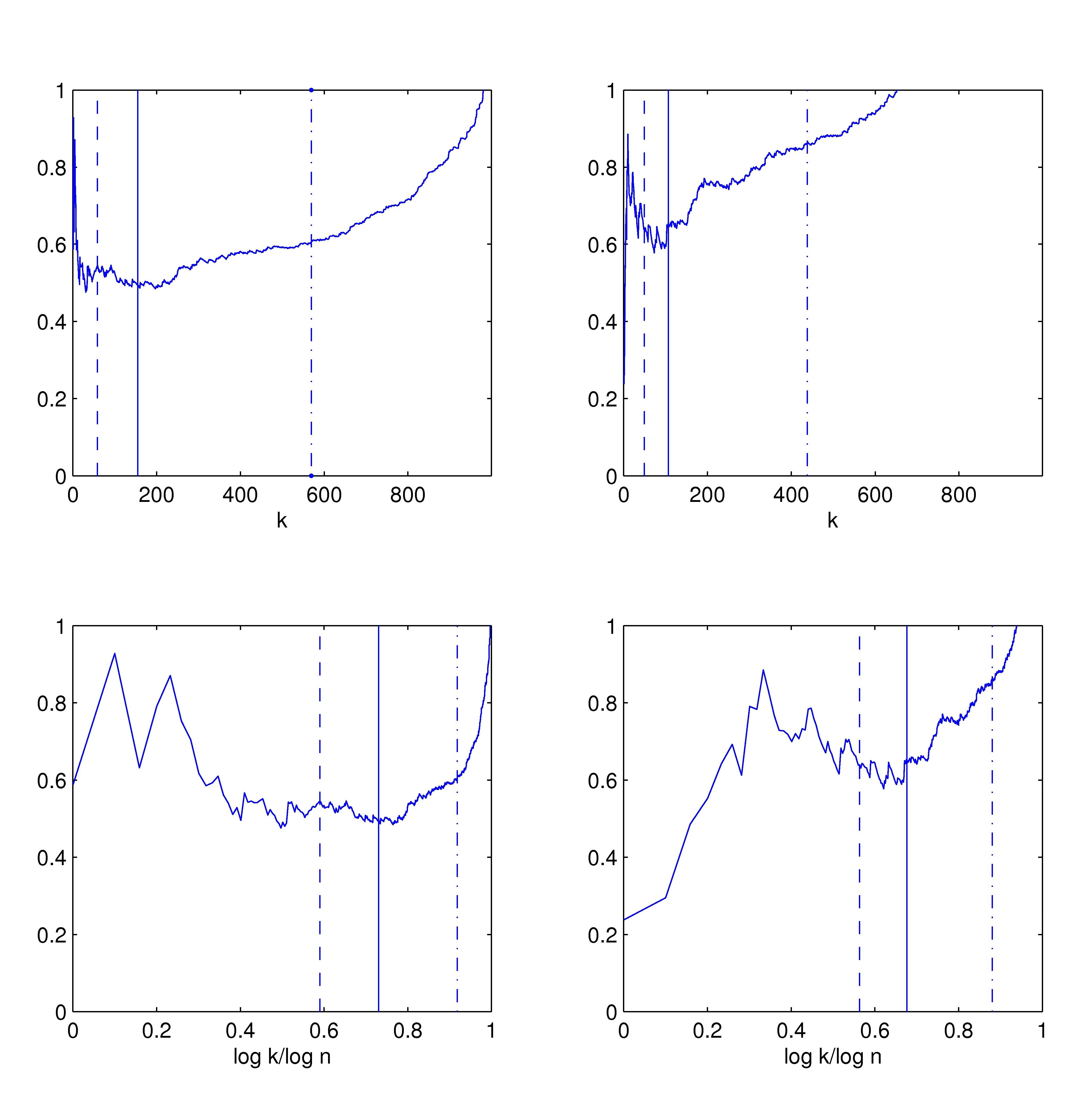
Figure 1: Hill estimator based on $k+1$ largest order statistics versus $k$ (above) and versus $\log k/\log n$ (below) for $n=1000$ iid Fréchet rv’s (left) and logarithmically disturbed Pareto rv’s (right) with $\gamma=1/2$. Estimated optimal numbers $\hat{k}_{n}^{boot}$ (dashed), $\hat{k}_{n}^{seq}$ (solid) and $\hat{k}_{n}^{ML}$ (dash-dotted) are indicated by vertical lines.

To give some advice how to choose the sample fraction used in the tail analysis in such cases and also to avoid subjective choices which have an influence on the estimation accuracy that is difficult to quantify, fully automatic data-driven selection procedures have been proposed that minimize the asymptotic mean squared error of the estimators under consideration. Here we consider three different methods to choose the number of largest order statistics such that the (asymptotic) mean squared error of the Hill estimator $\gamma_{n,k}$ is minimized. See Section 4.7 of Beirlant et al. (2004) for a more extensive list and additional references.

Danielsson et al. (2001) used a bootstrap approach to minimize the mean squared error (MSE). Hill (1990) showed that the standard bootstrap does not work here, because it does not capture the bias of the Hill estimator (and other linear statistics) properly, but a suitable bootstrap may yield a consistent estimator of the MSE in a restricted model. Instead of trying to minimize the MSE of the Hill estimator directly, Danielsson et al. (2001) used the auxiliary statistic $A_{n,k}:=(M_{n,k}-2\hat{\gamma}_{n,k}^{2})^{2}$ with

$$M_{n,k}:=k^{-1}\sum_{i=1}^{k}\log^{2}(X_{n-i+1:n}/X_{n-k:n}).$$ (4.1)

It can be shown that under a suitable second order condition, that generalizes assumption (3.14), a sequence $\bar{k}_{0}(n)$ which minimizes $E(A_{n,k})$ and a sequence $k_{0}(n)$ which minimizes the MSE of the Hill estimator $\hat{\gamma}_{n,k}$ have the same asymptotic behavior up to a multiplicative constant. Starting from this fact, Danielsson et al. (2001) developed the following algorithm:

• For some $\varepsilon\in(0,1/2)$, some $n_{1}=O(n^{1-\varepsilon})$ and $n_{2}:=[n_{1}^{2}/n]$, define $k_{0}^{*}(n_{i})$, $i=1,2$, which minimizes the conditional expectation of $(M_{n,k}^{*}-2(\hat{\gamma}_{n,k}^{*})^{2})^{2}$ given the data $X_{1},\ldots,X_{n}$, where $\hat{\gamma}_{n,k}^{*}$ and $M_{n,k}^{*}$ are defined as in (3.4) and (4.1), respectively, but with $n$ replaced by $n_{1}$ and $X_{i}$ replaced by $X_{i}^{*}$ independently drawn from $X_{1},\ldots,X_{n}$ (with replacement). Here the conditional expectation is minimized over $k_{1}\in\{[\log n_{1}],\ldots,[n_{1}/\log n_{1}]\}$, say.

• The asymptotic MSE of the Hill estimator $\hat{\gamma}_{n,k}$ is then minimal for

  $$\hat{k}_{n}^{boot}:=\frac{(k_{0}^{*}(n_{1}))^{2}}{k_{0}^{*}(n_{2})}\big{(}2\log n_{1}/\log k_{0}^{*}(n_{1})-1\big{)}^{2(\log k_{0}^{*}(n_{1})/\log n_{1}-1)}.$$

The performance of the data-driven choice of $k$ crucially depends on the value $n_{1}$. Using heuristic arguments, Danielsson et al. (2001) proposed to select $n_{1}$ which minimizes $(Q(n_{1},k_{0}^{*}(n_{1})))^{2}/$ $Q(n_{2},k_{0}^{*}(n_{2}))$ with $Q(n_{i},k_{i})$ denoting the conditional expectation of $\big{(}M_{n_{i},k_{i}}^{*}-2(\hat{\gamma}_{n_{i},k_{i}}^{*})^{2}\big{)}^{2}$ given the data.

Drees and Kaufmann (1998) suggested a sequential procedure that was inspired by the so-called Lepskii-method for adaptive bandwidth selection in curve estimation. The basic idea of this approach is that too large a difference between two Hill estimators $\hat{\gamma}_{n,i}$ and $\hat{\gamma}_{n,k}$ with $i<k$ indicates that the latter exhibits a large bias. As the random error of the difference is of the order $i^{-1/2}$, an asymptotically optimal choice of the number of order statistics can be determined from the smallest $k$ such that $i^{1/2}|\hat{\gamma}_{n,i}-\hat{\gamma}_{n,k}|$ exceeds a suitable threshold. More precisely, Drees and Kaufmann (1998) proposed the following algorithm:

• For some $r_{n}=o(n^{1/2})$ such that $(\log\log n)^{1/2}=o(r_{n})$ let

  $$\bar{k}_{n}(r_{n}):=\min\big{\{}k\in\{1,\ldots,n\}\mid\max_{1\leq i\leq k}i^{1/2}|\hat{\gamma}_{n,i}-\hat{\gamma}_{n,k}|>r_{n}\big{\}}.$$

• Fix some $\lambda,\xi\in(0,1)$ such that $(\log\log n)^{1/(2\xi)}=o(r_{n})$ and calculate a pilot estimate $\hat{\gamma}_{n}=\hat{\gamma}_{n,[2\sqrt{n^{+}}]}$ with $n^{+}$ denoting the number of positive observations. Then the asymptotic MSE of the Hill estimator $\hat{\gamma}_{n,k}$ is minimal for

  $$\hat{k}_{n}^{seq}:=\bigg{[}(2\hat{\rho}_{n}+1)^{-1/\hat{\rho}_{n}}(2\hat{\gamma}_{n}\hat{\rho}_{n})^{1/(2\hat{\rho}_{n}+1)}\Big{(}\frac{\bar{k}_{n}(r_{n}^{\xi})}{(\bar{k}_{n}(r_{n}))^{\xi}}\Big{)}^{1/(1-\xi)}\bigg{]}$$

  with

  $$\hat{\rho}_{n}:=\log\frac{\max_{1\leq i\leq[\lambda\bar{k}_{n}(r_{n})]}i^{1/2}\big{|}\hat{\gamma}_{n,i}-\hat{\gamma}_{n,[\lambda\bar{k}_{n}(r_{n})]}\big{|}}{\max_{1\leq i\leq\bar{k}_{n}(r_{n})}i^{1/2}\big{|}\hat{\gamma}_{n,i}-\hat{\gamma}_{n,\bar{k}_{n}(r_{n})}\big{|}}\Big{/}\log\lambda-\frac{1}{2}.$$

Here the specific values of $r_{n}$, $\xi$ and (to a lesser extent) $\lambda$ influence the performance of the procedure. the authors recommended to choose $r_{n}=2.5\hat{\gamma}_{n}n^{1/4}$, $\xi=0.7$ and $\lambda=0.8$; see Drees and Kaufmann (1998) for further comments on the implementation of this algorithm.

In yet another approach, Beirlant et al. (2004), Section 4.7.1 (ii), fitted an extended Pareto model with an explicit second order correction term to the data using a maximum likelihood estimator. Then they calculated and minimized the MSE of the Hill estimator directly from this fit. The resulting estimated optimal number will be denoted by $\hat{k}_{n}^{ML}$.

In Figure 1 the resulting estimates for the optimal number of order statistics are indicated by vertical lines. While the bootstrap (dashed line) and the sequential approach (solid line) both yield reasonable values, the method which uses an explicit model for the second order term leads to too large values and thus a considerable bias. Indeed, it has been observed in literature that for moderate sample sizes it is notoriously difficult to estimate the second order parameters like $\rho$ in expansion (3.14). In contrast, the bootstrap and the sequential approach both use estimates of this second order parameter only in an estimate of a multiplicative constant, while their order of magnitude does not explicitly depend on such an estimate. Hence they yield reasonable estimates even if this second order parameter is fixed (e.g., $\rho=1$) and misspecified.

Once the sample fraction of largest order statistics has been chosen, one should check whether it can be well approximated by a (generalized) Pareto distribution. A classical graphical tool for such an model validation is the qq-plot. If $F\in D(G_{\gamma})$ for some $\gamma>0$ and $k$ is chosen not too large, then using (2.6) one can approximate

$$\log\frac{X_{n-i+1:n}}{X_{n-k:n}}\approx\log\frac{{F^{\leftarrow}}(1-(i-1/2)/n)}{{F^{\leftarrow}}(1-(k+1/2)/n)}\approx-\gamma\log\frac{i-1/2}{k+1/2}.$$

Hence the points $\big{(}-\log((i-1/2)/(k+1/2)),\log(X_{n-i+1:n}/X_{n-k:n})\big{)}$ should approximately lie on the line with slope $\hat{\gamma}_{n}=T(Q_{n})$ through the origin. To assess whether the observed deviations of the points from this line are probably only due to their randomness or whether they indicate that the GPD approximation is inaccurate, we can again use Theorem 3.1.

Corollary 4.1.

Assume that $(k_{n})_{n\in\mathbb{N}}$ is an intermediate sequence such that condition (3.13) holds for some $\gamma>0$. Then for all $\varepsilon>0$ and all scale invariant functionals $T$ on $D_{\gamma,\varepsilon}$ satisfying $T(z_{\gamma})=\gamma$ and the differentiability condition (3.8), we have

$$k_{n}^{1/2}\Big{(}\log\frac{Q_{n}(t)}{Q_{n}(1)}+T(Q_{n})\log t\Big{)}_{0<t\leq 1}$$ (4.2)

$$\longrightarrow \Big{(}\gamma(t^{-1}W(t)-W(1))+\int_{(0,1]}s^{-(\gamma+1)}W(s)\,\nu_{T,\gamma}(ds)\cdot\log t\Big{)}_{0<t\leq 1}$$

weakly in $\big{(}D_{0,\varepsilon},\|\cdot\|_{0,\varepsilon}\big{)}$. Hence,

$$P\Big{\{}\max_{1\leq i\leq k_{n}}h\Big{(}\frac{i-1/2}{k_{n}+1/2}\big{)}\Big{|}\log\frac{X_{n-i+1:n}}{X_{n-k_{n}:n}}+T(Q_{n})\log\frac{i-1/2}{k_{n}+1/2}\Big{|}>c\Big{\}}$$ (4.3)

$$\longrightarrow P\Big{\{}\sup_{0<t\leq 1}h(t)\Big{|}\gamma(t^{-1}W(t)-W(1))+\int_{(0,1]}s^{-(\gamma+1)}W(s)\,\nu_{T,\gamma}(ds)\cdot\log t\Big{|}>c\Big{\}}$$

for all continuous functions $h:(0,1]\to(0,\infty)$ such that $h(t)t^{-(1/2+\varepsilon)}\to 0$ as $t\downarrow 0$ for some $\varepsilon>0$. In particular, for $T=T_{H}$ (i.e., $T(Q_{n})$ equal to the Hill estimator), we obtain

$$P\Big{\{}\max_{1\leq i\leq k_{n}}h\Big{(}\frac{i-1/2}{k_{n}+1/2}\big{)}\Big{|}\log\frac{X_{n-i+1:n}}{X_{n-k_{n}:n}}+T_{H}(Q_{n})\log\frac{i-1/2}{k_{n}+1/2}\Big{|}>cT_{H}(Q_{n})\Big{\}}$$ (4.4)

$$\longrightarrow P\Big{\{}\sup_{0<t\leq 1}h(t)\Big{|}t^{-1}W(t)-W(1)+\int_{(0,1]}s^{-1}W(s)-W(1)\,ds\cdot\log t\Big{|}>c\Big{\}}.$$

Under slightly different conditions, a similar result has been proved by Dietrich et al. (2002) for the Hill estimator.

Using (4.4) one can turn the Pareto qq-plot into a statistical testing tool with given asymptotic size $\alpha$. To this end, for some function $h$ satisfying the conditions of Corollary 4.1, using Monte Carlo simulations, one determines a critical value $c_{\alpha}$ such that the probability on the right-hand side of (4.4) equals $\alpha$. Then with probability of about $1-\alpha$ all points of the Pareto qq-plot should lie in the band defined by the graphs of the functions $T_{H}(Q_{n})(\log t\pm c_{\alpha}/h(t))$ if the GPD approximation is accurate enough so that the bias of the Hill estimator is negligible. The choice of the function $h$ determines in which part of the qq-plot deviations are most easily detected: the larger $h(t)$ is, the more narrow is the band at that point. Because of the condition $h(t)t^{-(1/2+\varepsilon)}\to 0$ as $t\downarrow 0$, the band always widens for small values of $t$, thus allowing for larger deviations of the most extreme points of the qq-plot from the ideal line.

It has been suggested to use such tests also to select the tail fraction to be analyzed by increasing $k$ until the test rejects the GPD hypothesis (see, e.g., Dietrich et al., 2002, Remark 2). In some applications this approach may be problematic if $\alpha$ is chosen as small as it is common in testing (e.g., $\alpha=0.05$). Note that the limiting Gaussian process in (4.2) tends to 0 as $t$ tends to 1, but that the function $h$ is assumed continuous and hence bounded, so that deviations of points of the qq-plot from the ideal line near $t=1$ (corresponding to the smallest order statistics taken into account) are usually difficult to detect. Hence it may happen that one increases the number $k$ so much that the Hill estimator (and other extreme value estimators) are strongly biased, before the tests acknowledges that the last order statistics taken into account are poorly fitted. (The same argument also applies if $L_{2}$-type tests like the one examined by Dietrich et al. (2002) are used.)

To avoid such effects, one might think of choosing a weight function $h$ that tends to $\infty$ as $t$ tends to 1 to compensate for the decrease of the modulus of the limiting Gaussian process. For instance, as this process has the variance function $\sigma^{2}(t)=t^{-1}-1-\log^{2}t$ if $T=T_{H}$, one might be tempted to use a weight function of the form $h(t)=(t(1-t))^{\varepsilon}/\sigma(t)$ for some small $\varepsilon>0$. Unfortunately, without additional conditions on the smoothness of ${F^{\leftarrow}}$, convergence (4.4) need not hold for such a choice of $h$. The reason is that under the general condition (2.5) small jumps of ${F^{\leftarrow}}$ (or continuous small but rapid changes) are still possible which lead to an “unusually” irregular behavior of the tail empirical quantile function $Q_{n}$ near 1. If one strengthens condition (2.5) to a regularity condition on the quantile density function $({F^{\leftarrow}})^{\prime}(1-t)=f({F^{\leftarrow}}(1-t))$, though, then assertion (4.2) may also be strengthened. It is well known that if ${F^{\leftarrow}}$ has a Lebesgue density which is monotonically decreasing in a neighborhood of 1, then by Karamata’s theorem

$$\eta(t):=\frac{tf({F^{\leftarrow}}(1-t))}{{F^{\leftarrow}}(1-t)}-\gamma\;\to\;0$$

(cf. de Haan and Ferreira (2006), Proposition B.1.9 11.). If we replace condition (3.13) with a condition on $k_{n}$ in terms of the function $\eta$, then convergence (4.2) can be made more precise in a neighborhood of $t=1$.

Corollary 4.2.

Assume that $(k_{n})_{n\in\mathbb{N}}$ is an intermediate sequence such that for some $\gamma>0$

$$k_{n}^{1/2}\sup_{0<t\leq(1+\tilde{\varepsilon})k_{n}/n}|\eta(t)|\;\to\;0$$ (4.5)

and that the functional $T$ satisfies the conditions specified in Corollary 4.1. Then for all $\varepsilon>0$ and for all continuous functions $h:(0,1)\to(0,\infty)$ such that $h(t)t^{-(1/2+\varepsilon)}\to 0$ as $t\downarrow 0$, and $h(t)(1-t)^{1/2-\varepsilon}\to 0$ as $t\uparrow 1$, one has

$$k_{n}^{1/2}\bigg{(}h(t)\Big{(}\log\frac{Q_{n}(t)}{Q_{n}(1)}+T(Q_{n})\log t\Big{)}1_{(0,1-1/(2k_{n})]}(t)\bigg{)}_{0<t<1}$$ (4.6)

$$\longrightarrow \bigg{(}h(t)\Big{(}\gamma(t^{-1}W(t)-W(1))+\int_{(0,1]}s^{-(\gamma+1)}W(s)\,\nu_{T,\gamma}(ds)\cdot\log t\Big{)}\bigg{)}_{0<t<1}$$

weakly with respect to the supremum norm. In particular, convergence (4.4) holds for $T=T_{H}$.

In Section 6 this result is applied to construct a “confidence band” for the Hill-qq-plot based on claim sizes from health insurances.

If one uses some estimator of $\gamma$ different from the Hill estimator, then usually the probability on the right-hand side of (4.3) is a continuous non-linear function of the unknown extreme value index $\gamma$. In that case, one can still construct tests with prescribed asymptotic size $\alpha$ for the null hypothesis that (3.13) holds. To this end, one first estimates $\gamma$ consistently by $\hat{\gamma}_{n}=T(Q_{n})$ and then, using Monte Carlo simulations, one determines a critical value $c_{\alpha}$ such that the right-hand side of (4.3) equals $\alpha$ when $\gamma$ is replaced with $\hat{\gamma}_{n}$.

Since the supremum is difficult to simulate, it seems natural to simulate the limiting process $Z(t)=t^{-1}W(t)-W(1)+\int_{(0,1]}s^{-(\gamma+1)}W(s)\,\nu_{T,\gamma}(ds)\cdot\log t$ on a fine grid $t_{i},1\leq i\leq m$, and then to approximate the supremum by $\max_{1\leq i\leq m}h(t_{i})|Z(t_{i})|$. This can still be computationally challenging if one tries to approximate the integral of $s^{-(\gamma+1)}W(s)$ using some quadrature formula, because the integrand is unbounded in a neighborhood of zero and a large number of integration points may be needed to obtain an accurate approximation. Fortunately, for most estimators, one can avoid numerical integration using the fact that conditionally on $W(t_{i})$, $1\leq i\leq m$, the integrals $\int_{(t_{i-1},t_{i}]}s^{-(\gamma+1)}W(s)\,\nu_{T,\gamma}(ds)$, $1\leq i\leq m$, (with $t_{0}:=0$) are independent normal rv’s with mean

$$\mu_{i} := \int_{(t_{i-1},t_{i}]}s^{-\gamma}\,\nu_{T,\gamma}(ds)\frac{W(t_{i})-W(t_{i-1})}{t_{i}-t_{i-1}}$$

$$\hskip 28.45274pt+\int_{(t_{i-1},t_{i}]}s^{-(\gamma+1)}\,\nu_{T,\gamma}(ds)\Big{(}W(t_{i-1})-\frac{t_{i-1}}{t_{i}-t_{i-1}}(W(t_{i})-W(t_{i-1}))\Big{)}$$

and variance

$$\sigma_{i}^{2}:=\frac{1}{t_{i}-t_{i-1}}\int_{(t_{i-1},t_{i}]}\int_{(t_{i-1},t_{i}]}(st)^{-(\gamma+1)}(\min(s,t)-t_{i-1})(t_{i}-\max(s,t))\,\nu_{T,\gamma}(ds)\,\nu_{T,\gamma}(dt).$$

This statement, in turn, follows from the conditional independence of the processes $(W(t))_{t_{i-1}\leq t\leq t_{i}}$ which have the same conditional distribution as

$$W(t_{i-1})-\frac{t_{i-1}}{t_{i}-t_{i-1}}(W(t_{i})-W(t_{i-1}))+\tilde{W}(t-t_{i-1})-\frac{t-t_{i-1}}{t_{i}-t_{i-1}}\tilde{W}(t_{i}-t_{i-1})$$

with $\tilde{W}$ denoting a Brownian motion independent of $W$. Hence the limiting Gaussian process $Z$ can be simulated as follows if integrals of power functions with respect to $\nu_{T,\gamma}$ can be calculated analytically:

1. Simulate $m$ independent centered normal rv’s $\Delta_{i}$ with variance $t_{i}-t_{i-1}$ where $t_{0}:=0$ and $t_{m}:=1$, and let $W(t_{l}):=\sum_{i=1}^{l}\Delta_{i}$.

2. Simulate a normal rv $I$ with mean $\sum_{i=1}^{m}\mu_{i}$ and variance $\sum_{i=1}^{m}\sigma_{i}^{2}$.

3. Then $\big{(}\gamma(t_{i}^{-1}W(t_{i})-W(t_{m}))+I\log t_{i})\big{)}_{1\leq i\leq m}$ is a (pseudo) realization of $(Z(t_{i}))_{1\leq i\leq m}$.

Note that the variance of $I$ does not depend on $W$. In case of the Hill estimator and equidistant design points $t_{i}=i/m$, one has

$$\sum_{i=1}^{m}\mu_{i} = (1+\log m)\Delta_{i}+\sum_{i=2}^{m}\Big{(}\log\frac{m}{i}+1-(i-1)\log\frac{i}{i-1}\Big{)}\Delta_{i}$$

$$\sum_{i=1}^{m}\sigma_{i}^{2} = 1-\frac{1}{m}\sum_{i=1}^{m-1}i(i+1)\log^{2}\frac{i+1}{i}.$$

The Corollaries 4.1 and 4.2 describe tests for the null hypothesis that the left-hand sides of (3.13) and (4.5), respectively, are negligible. Likewise, one can devise analogous tests for the validity of condition (3.6), but the resulting limiting process is more complicated.

Corollary 4.3.

Suppose that $(k_{n})_{n\in\mathbb{N}}$ is an intermediate sequence satisfying condition (3.6) for some $\gamma\geq 0$, and that $S,T:D_{\gamma,\varepsilon}\to\mathbb{R}$ are scale and location invariant functionals such that $S(z_{\gamma})=1$, $T(z_{\gamma})=\gamma$ and the differentiability conditions (3.8) and (3.11) are met. Then for all $\varepsilon>0$

$$k_{n}^{1/2}\Big{(}\log\frac{Q_{n}(t)-Q_{n}(1)}{S(Q_{n})}+-\frac{t^{-T(Q_{n})}-1}{T(Q_{n})}\Big{)}_{0<t\leq 1}\;\longrightarrow\;\Big{(}t^{-(\gamma+1)}W(t)-W(1)$$

$${}-\int_{(0,1]}s^{-(\gamma+1)}W(s)\,\nu_{T,\gamma}(ds)\cdot\frac{1-t^{-\gamma}(1+\gamma\log t)}{\gamma^{2}}-\int_{(0,1]}s^{-(\gamma+1)}W(s)\,\nu_{S,\gamma}(ds)\cdot\frac{t^{-\gamma}-1}{\gamma}\Big{)}_{0<t\leq 1}$$

weakly in $\big{(}D_{\gamma,\varepsilon},\|\cdot\|_{\gamma,\varepsilon}\big{)}$ (with $(1-t^{-\gamma}(1+\gamma\log t))/\gamma^{2}$ interpreted as $(\log^{2}t)/2$ for $\gamma=0$).

The proof is omitted as the assertion follows readily from Theorem 3.1, (3.10), (3.12) and a Taylor expansion of $\gamma\mapsto(t^{-\gamma}-1)/\gamma$.

Similarly as above, from Corollary 4.3 one may construct bands around the fitted generalized Pareto quantile function $Q_{n}(1)+S(Q_{n})(t^{-T(Q_{n})}-1)/T(Q_{n})$ in which all the points $\big{(}(i-1/2)/(k_{n}+1/2),X_{n-i+1:n}\big{)}$ should lie with probability of about $1-\alpha$.

5 Analysis of the extremal dependence

In recent years, the analysis of the dependence between the extremes of the components of a random vector of risks has attracted much attention. If the random vector describes returns on different assets, then it is obviously important to assess the risk of large losses in different assets at the same time. However, extremal dependence also matters in the analysis of claim sizes from one customer in different lines of business. For example, if both a building and its content are insured with the same company, then a fire will often lead to large claims in both lines of business. Likewise, some dependence can be expected between the claims in different types of health insurances (e.g.  inpatient and outpatient cover); cf. Section 6.

In order not to overload this presentation, we will only sketch the basic theory used in the analysis of extremal dependence, but we will rather discuss some pitfalls and problems that may arise in applications in more detail. For simplicity, we mainly consider bivariate vectors $(X_{1},X_{2})$ of claim sizes (or risks).

Analogously to our basic assumption (2.1) in the univariate setting, in classical multivariate extreme value theory it is assumed that the conditional distribution of the suitably standardized random vector given that its norm exceeds a high threshold converges to a non-degenerate limit as the threshold increases. However, as the components of the vector need not be of comparable size, the marginal distributions are usually first standardized, e.g., to the standard Pareto distribution:

$$Y:=\Big{(}\frac{1}{1-F_{l}(X_{l})}\Big{)}_{1\leq l\leq 2}.$$ (5.1)

Here we assume for simplicity that the marginal cdf’s $F_{l}$, $1\leq l\leq 2$, of $X$ are continuous.

Now fix some norm $\|\cdot\|$ on $\mathbb{R}^{2}$ and suppose that

$$P\Big{(}\frac{Y}{u}\in\cdot\,\Big{|}\,\|Y\|>u\Big{)}\;\longrightarrow\;P^{Z}(\cdot)\quad\text{weakly}$$ (5.2)

as $u\to\infty$ for some non-degenerate limit distribution $P^{Z}$. In that case, $Y$ and $P^{Y}$ are said to be multivariate regularly varying.

It can be shown that this condition does not depend on the specific choice of the norm, while the exact form of the limit distribution does. For example, if one works with the maximum norm $\|\cdot\|_{\infty}$, then (5.2) is equivalent to

$$P(Y_{1}>uy_{1}\text{ or }Y_{2}>uy_{2}\mid Y_{1}>u\text{ or }Y_{2}>u) = \frac{1-F_{Y}(uy_{1},uy_{2})}{1-F_{Y}(u,u)}$$ (5.3)

$$\to P\{Z_{1}>y_{1}\text{ or }Z_{2}>y_{2}\}$$

$$=: 1-H(y_{1},y_{2})$$

for all points $(y_{1},y_{2})\in[1,\infty)^{2}$ of continuity of $H$.

Applying the (generalized) polar transformation

$$\Xi:y\mapsto\Big{(}\|y\|,\frac{y}{\|y\|}\Big{)},$$

one can conclude from (5.2) that

$$P\Big{(}\Big{(}\|Y\|,\frac{Y}{\|Y\|}\Big{)}\in\cdot\,\Big{|}\,\|Y\|>u\Big{)}\;\longrightarrow\;P^{\Xi(Z)}(\cdot)\quad\text{weakly.}$$

Now standard arguments from the theory of regular variation show that the limiting distribution $P^{\Xi(Z)}$ must be a product measure with first factor equal to the standard Pareto distribution and the second factor being some distribution $\Phi$ on the upper right quadrant $S^{+}:=\{z\in[0,\infty)\mid\|z\|=1\}$ of the unit “circle” with respect to the norm $\|\cdot\|$. Unlike in the univariate setting, all possible limit distributions do not form a parametric family, because the so-called spectral probability measure $\Phi$ can be any distribution on $S^{+}$ satisfying the condition

$$\int_{S^{+}}\omega_{1}\,\Phi(d\omega)=\int_{S^{+}}\omega_{2}\,\Phi(d\omega),$$ (5.4)

that follows from the fact that all marginal cdf’s are standard Pareto.

Remark 5.1.

In the literature, instead of (5.2) often the equivalent assumption

$$uP\Big{\{}\frac{Y}{u}\in\cdot\,\Big{\}}\,\longrightarrow\,\nu\quad\text{vaguely as }u\to\infty$$ (5.5)

is considered, where $\nu$ is some Radon measure on $[0,\infty]^{2}\setminus\{(0,0)\}$ (see e.g. Resnick (2007), Section 6.1). Similarly as before, one can conclude that the measure $\nu^{\Xi}$ induced by the polar transformation is the product of the measure with Lebesgue density $t\mapsto t^{-2}$ on $(0,\infty)$ and a finite measure $\tilde{\Phi}$ on $S^{+}$, the so-called spectral measure. The latter is related to the spectral probability measure via

$$\Phi=\frac{\tilde{\Phi}}{\tilde{\Phi}(S^{+})}\quad\text{and}\quad\tilde{\Phi}=\frac{\Phi}{\int_{S^{+}}\omega_{1}\,\Phi(d\omega)}.$$

For an arbitrary measurable set $A\subset(0,\infty)^{2}$ one has

$$P\Big{(}\frac{Y}{u}\in A\,\Big{|}\,\|Y\|>u\Big{)}\;\longrightarrow\;\int_{S^{+}}\int_{1}^{\infty}1_{A}(t\omega)t^{-2}\,dt\,\Phi(d\omega)$$ (5.6)

as $u\to\infty$, provided the set $A$ is continuous with respect to the limit measure (that is the right-hand side equals 0 if $A$ is replaced with its topological boundary). Hence, to estimate the probability that some future observation $X$ falls into a given extreme set $C$ (e.g., $C=(x_{1},\infty)\times(x_{2},\infty)$ describing the event that the claim sizes in both lines of business exceed a given high threshold) can be estimated as follows:

1. Estimate the marginal cdf’s $F_{l}$ by $\hat{F}_{l}$; for the estimation of the tails, the methods discussed in the previous sections can be used.

2. Transform the data $X_{i}=(X_{i,1},X_{i,2})$, $1\leq i\leq n$, and the extreme set $C$ using the fitted marginal cdf’s:

   $$\hat{Y}_{i} := \Big{(}\frac{1}{1-\hat{F}_{1}(X_{i,1})},\frac{1}{1-\hat{F}_{2}(X_{i,2})}\Big{)}$$

   $$\frac{1}{1-\hat{F}(C)} := \Big{\{}\Big{(}\frac{1}{1-\hat{F}_{1}(x_{1})},\frac{1}{1-\hat{F}_{2}(x_{2})}\Big{)}\,\Big{|}\,(x_{1},x_{2})\in C\Big{\}}.$$

3. Fix some norm and estimate the corresponding spectral probability measure $\Phi$ by $\hat{\Phi}$ (see below).

4. Use (5.6) and the regular variation of $\|Y\|$ to approximate

   $$P\{X\in C\} = P\Big{\{}Y\in\frac{1}{1-F(C)}\Big{\}}$$

   $$= P\Big{(}Y\in\frac{1}{1-F(C)}\,\Big{|}\,\|Y\|>ru\Big{)}\cdot\frac{P\{\|Y\|>ru\}}{P\{\|Y\|>u\}}\cdot P\{\|Y\|>u\}$$

   $$\approx \int_{S^{+}}\int_{1}^{\infty}1_{1/(1-F(C))}(t\omega)t^{-2}\,dt\,\Phi(d\omega)\cdot r^{-1}\cdot P\{\|Y\|>u\}$$

   $$\approx \int_{S^{+}}\int_{1}^{\infty}1_{1/(1-\hat{F}(C))}(t\omega)t^{-2}\,dt\,\hat{\Phi}(d\omega)\cdot r^{-1}\cdot\frac{1}{n}\sum_{i=1}^{n}1_{\textstyle\{\|\hat{Y}_{i}\|>u\}}.$$

   Here we have assumed that $\|y\|>ru$ for all $y\in 1/(1-F(C))$, while on the other hand $ru$ is sufficiently large such that (5.6) (with $ru$ instead of $u$) yields a good approximation. Moreover, on the one hand $u$ must be sufficiently large such that $P\{\|Y\|>ru\}/P\{\|Y\|>u\}\approx r^{-1}$, while on the other hand it must be sufficiently small such that $P\{\|Y\|>u\}$ can be well estimated by its empirical counterpart.

As the family of all possible spectral (probability) measures is nonparametric (infinite dimensional), it is substantially more complicated to estimate $\Phi$ (or $\tilde{\Phi}$) than to fit the tail of a univariate cdf. In the last decade, though, a variety of nonparametric estimators of the spectral measure and related functions, that also characterize the extremal dependence structure, have been suggested and analyzed; see, for instance, de Haan and Ferreira (2006), Chapter 7, Beirlant et al. (2004), Chapter 9, or Einmahl and Segers (2009). These estimators also use marginally transformed observations $\hat{Y}_{i}$, but, unlike in program to estimate the probability of extreme events outlined above, here one may use fully nonparametric estimators of the marginal cdf’s, which amounts to working with the coordinatewise ranks of the original observations. In the analysis of the asymptotic behavior of these estimators, it is important to not assume that the marginal cdf’s are known, because usually the transformation of the data using estimated marginal cdf’s (rather than the true ones) does have a non-negligible influence on the estimation error for $\Phi$; ignoring it may lead to a wrong assessment of the estimation accuracy (see, e.g., Einmahl and Segers (2009), p. 2960).

As an alternative approach, it has been suggested to assume some parametric submodel of spectral (probability) measures and then to fit this model to the transformed observations using maximum likelihood or a generalized moment method. Sometimes it is even assumed that, for some $\Phi$ from this parametric family, in (5.6) equality holds for some sufficiently large $u$. We consider this approach quite problematic, because it will rarely be possible to argue for a specific parametric family of spectral measures based on either experience with similar data sets or some “physical” reasoning about the process generating the extremal dependence. Instead, the parametric families are almost always chosen with mathematical convenience in view, while it is argued that the family is sufficiently flexible to capture many different dependence structures. Then, however, one merely trades the random estimation error, that can be quantified in the nonparametric framework, for the risk of a model misspecification, that can hardly be assessed. Hence the seemingly increased estimation accuracy which comes with the parametric approach if the model is correct will often be just a chimera, which possibly leads to an assessment of the insured risk which is not prudent anymore.

An even more restrictive modeling approach is related to a reformulation of the multivariate regular variation in terms of copulas. Any multivariate cdf $F$ with marginal cdf’s $F_{l}$, $1\leq l\leq d$, can be represented as $F(x_{1},\ldots,x_{l})=C(F_{1}(x_{1}),\ldots,F_{d}(x_{d}))$ where $C$ is a so-called copula, i.e. a multivariate cdf with uniform margins. If all $F_{l}$ are continuous, then $C$ is unique: it is the joint cdf of $(F_{1}(X_{1}),\ldots,F_{d}(X_{d}))$. Thus, the cdf $F_{Y}$ of $Y$ defined by (5.1) equals $F_{Y}(y_{1},y_{2})=C(1-1/y_{1},1-1/y_{2})$ and convergence (5.3) is equivalent to

$$\lim_{t\downarrow 0}\frac{1-C(1-ty_{1},1-ty_{2})}{1-C(1-t,1-t)}=1-H(y_{1}^{-1},y_{2}^{-1})$$

for all points $(y_{1}^{-1},y_{2}^{-1})$ of continuity of $H$. Hence the parametric approach outlined above boils down to assuming that, on a small neighborhood of the point (1,1), the copula $C$ can be well approximated by a parametric model.

Because the estimation of a general copula is essentially as difficult as the estimation of a general multivariate cdf (in particular it is also plagued by the well-known “curse of dimensionality”), it has been suggested to assume parametric models for the whole copula $C$. This approach, however, does not only introduce a modeling error that is difficult to quantify, but it contradicts the general philosophy of extreme value theory to “let the tails speak for themselves”. In contrast, while the estimation error of the aforementioned nonparametric estimators of the extremal dependence structure can be quite large (in particular in higher dimensions), it can be well assessed under weak model assumptions and thus it can be taken into account by the risk manager. For that reason, with the rare exception of those situations when there are convincing arguments that a particular family of copulas contains the true one (and not just a crude approximation to it), one should take the utmost care in analyzing the tail risk using parametric copulas, in particular in actuarial applications where prudence is a time-honored principle. (In this context, the interested reader is advised to study the article by Mikosch (2006) and the pertaining discussion for an enlightening and entertaining argument about the pros and cons of copula modeling.)

While the program sketched above in four steps will often yield a reasonable assessment of the risk that a future observation falls into some given extreme set if some nonparametric estimator of $\Phi$ is used, there is one important case in which the result can be quite misleading. Suppose that large values of one component of the transformed vector $Y$ of risks do not usually coincide with large values of the other component, or more precisely that

$$P(Y_{2}>u\mid Y_{1}>u)\;\to\;0$$ (5.7)

as $u\to\infty$. In that case, $X_{1}$ and $X_{2}$ (or $Y_{1}$ and $Y_{2}$) are said to be asymptotically independent. Straightforward calculations show that then the limit measure $\nu$ in (5.5) has no mass on $(0,\infty]^{2}$, i.e., it is concentrated on the axes. Hence, $\tilde{\Phi}$ and $\Phi$ have mass only in the points $(0,1)$ and $(1,0)$ if one uses one of the usual $p$-norms on $\mathbb{R}^{2}$ with $p\in[1,\infty]$. (Indeed, because of the normalization constraint (5.4), $\Phi$ must be the uniform distribution on $\{(0,1),(1,0)\}$.) But then for all sets $A$ that do not intersect with any of the axes, the limit in (5.6) is 0, which usually is too crude an approximation for the left-hand side.

Note that asymptotic independence is a property of the copula of $X$. Many popular parametric families of copulas allow for asymptotic independence for suitable parameter values. A thorough analysis of the tail behavior of so-called Archimedean copulas both in the case of asymptotic independence and of asymptotic dependence can be found in Charpentier and Segers (2009).

To obtain more useful approximations, one has to specify the rate at which $P(Y_{2}>u\mid Y_{1}>u)$ tends to 0. More precisely, one assumes that for some nontrivial function $d$

$$\frac{P\{Y_{1}>uy_{1},Y_{2}>uy_{2}\}}{P\{Y_{1}>u,Y_{2}>u\}}\;\to\;d(y_{1},y_{2})$$ (5.8)

as $u\to\infty$ uniformly for all points $(y_{1},y_{2})$ with $\max(y_{1},y_{2})=1$. As an immediate consequence, one obtains the regular variation of the function $u\mapsto P\{Y_{1}>u,Y_{2}>u\}=P\{\min(Y_{1},Y_{2})>u\}$:

$$\frac{P\{\min(Y_{1},Y_{2})>ux\}}{P\{\min(Y_{1},Y_{2})>u\}}\;\to\;x^{-1/\eta}$$ (5.9)

as $u\to\infty$ for all $y_{1},y_{2}>0$ and some $\eta\in(0,1]$ which is called the coefficient of tail dependence. Moreover, the limiting function $d$ is homogeneous of order $-1/\eta$. Since $Y_{1}$ and $Y_{2}$ are asymptotically independent whenever $P\{Y_{1}>u,Y_{2}>u\}=o(u)$, in particular one has asymptotic independence if $\eta<1$. If $Y_{1}$ and $Y_{2}$ are exactly independent, then $\eta=1/2$, while, roughly speaking, values of $\eta$ between 1/2 and 1 indicate a positive, but asymptotically vanishing dependence between the large values of $Y_{1}$ and $Y_{2}$. A slight modification of this model was first suggested by Ledford and Tawn (1996,1997).

To construct estimators of the coefficient of tail dependence, let $\hat{Y}_{i,l}^{(n)}:=(n+1)/(n+1-R_{i,l})$, $1\leq i\leq n,1\leq l\leq 2$, with $R_{i,l}$ denoting the rank of $X_{i,l}$ among $X_{1,l},\ldots,X_{n,l}$. Hence $\hat{Y}_{i,l}^{(n)}=1/(1-\hat{F}_{l}(X_{i,l}))$ where $\hat{F}_{l}$ is essentially the empirical cdf of $X_{1,l},\ldots,X_{n,l}$, with a minor modification to avoid division by 0. In view of (5.9), the rv’s

$$T_{i}^{(n)}:=\min\big{(}\hat{Y}_{i,1}^{(n)},\hat{Y}_{i,2}^{(n)}\big{)}$$ (5.10)

have approximately a Pareto tail with extreme value index $\eta$, that can be estimated by one of the usual estimators discussed in Section 3 applied to $T_{i}^{(n)}$, $1\leq i\leq n$. Draisma et al. (2004) proved an analog to Theorem 3.1 for the tail empirical quantile function pertaining to these rv’s. It turned out that in case of asymptotic independence one obtains the same limit as in Theorem 3.1, so that also all the results on the extreme value estimators discussed in Section 3 carry over to the present situation (although the rv’s $T_{i}^{(n)}$ are not exactly independent). If the components are not asymptotically independent, one can still conclude the asymptotic normality of the estimators of $\eta$, but the formulas for the asymptotic variance are more complicated and depend on the positive limit of $P(Y_{2}>u\mid Y_{1}>u)$.

Drees and Müller (2008) proposed the estimator

$$\hat{d}(y_{1},y_{2}):=\frac{1}{m}\sum_{i=1}^{n}1_{\textstyle\{\hat{Y}_{i,1}>T^{(n)}_{n-m:n}y_{1},\hat{Y}_{i,2}>T^{(n)}_{n-m:n}y_{2}\}}$$ (5.11)

of the limiting function $d(y_{1},y_{2})$ in (5.8) and proved uniform convergence of the suitably standardized estimation error $\hat{d}-d$ towards a centered Gaussian process under suitable smoothness conditions on $d$. Moreover, they derived statistical tests and a graphical tool to validate the model assumption (5.8). Finally, the theory was applied to two well-known bivariate data sets of claim sizes, the first describing losses to buildings and losses to their content in Danish fire insurances, while the second was taken from the Society of Actuaries Group Medical Insurance Large Claims Database (cf. Section 6). In both cases it seems very likely that condition (5.8) holds with a coefficient of tail dependence $\eta$ less than 1. As the point estimates of $\eta$ were larger than 1/2, the claim sizes in the different lines of business are probably asymptotically independent, though with a non-negligible positive dependence for finite levels. Applying classical bivariate extreme value theory in such cases will usually lead to a wrong assessment of the true risk insured.

So far, the extremal dependence structure has been analyzed in terms of the joint distribution of the observations after a standardization of the marginals to some fixed distribution (standard Pareto or uniform). Consequently both coordinates of the random vector have been treated symmetrically. As an alternative, in recent years the so-called conditional extreme value (CEV) approach has been considered, where the asymptotic behavior of one component (after a suitable linear normalization) given that the other component is large is investigated. For example, Abdous et al. (2005) and Abdous et al. (2008) considered the limit behavior of

$$P\big{(}X_{2}\leq a(x_{i})x_{2}+b(x_{1})\mid X_{1}>x_{1}\big{)}$$ (5.12)

as $x_{1}\to\infty$ for elliptically distributed vectors $(X_{1},X_{2})$, and Fougères and Soulier (2010) determined such limit distributions for more general bivariate distributions in polar representation. Das and Resnick (2011) examined possible limits in (5.12) in a general framework of regular variation on cones and discussed the relationship to the approach by Ledford and Tawn. In the special case $a(x_{1})=1$ and $b(x_{1})=0$ (coined standard regular varying case by Das and Resnick), the CEV approach facilitates the analysis of the extremal dependence between large claim sizes in absolute terms rather than just a comparison the behavior of the conditional distribution of one claim size given that the other is large relative to its unconditional distribution as in the approach by Ledford and Tawn. Unfortunately, in most applications one needs different normalizing functions $a$ and $b$ to obtain a non-degenerate limit of (5.12).

It is worth mentioning that the methods outlined in this section are only useful to analyze the dependence between extreme claim sizes (or losses) observed in a small number of different lines of insurances (usually sold to the same customer). From an economic point of view, the dependence between different risks insured in the same line of business is often more important. For example, in property insurance a large storm will usually result in many claims from customers living in the same area. With the present state of the art, extreme value theory has little to offer to analyze the extremal dependence in such situations. Instead, approaches using expert knowledge (e.g., from meteorology) remain the methods of choice.

6 Analyzing Large Claim Sizes in Health Insurance

In the years 1991 and 1992 the Society of Actuaries collected large claim sizes (totalling $25,000 or more) in US health insurances. The resulting large claim size database is available at the website http://www.soa.org. For each claimant, hospital charges and other charges were recorded in each year together with the type of the health insurance plan and the status of the claimant (employee or dependent), among other information. See Grazier and G’Sell Associates (1997) for a detailed description of the data set (see also Cebrián et al. (2003) for a statistical analysis of the total charges).

A closer inspection of the data reveals that the structure of the claim sizes depend on the status of the claimant and the type of the health insurance plan. For example, the large non-hospital costs were significantly larger for HMO (health maintenance organization), POS (point of service) and indemnity plans than for PPO (preferred provider organization), EPO (exclusive provider organization), comprehensive and other indemnity plans as well as for those records for which the type of plan was unknown. Therefore, as an example here we analyze the claims for the second group of health plans in the year 1992 when the claimant had the status ‘dependent’.

The sampling scheme that only those claims with total costs of at least $25,000 were recorded introduces an artificial negative dependence between both components: if the hospital charges were small, say less than $5,000, then the other charges must be larger than $20,000, and vice versa. For that reason, here we only consider those records for which both type of charges were at least $25,000, leading to a sample of size $n=1959$. (We discuss the consequences of this choice at the end of the section.)

First we fit Pareto distributions to the marginal tails. Figure 2 shows the maximum likelihood estimator (in the GPD model) for the extreme value index of the hospital charges (solid line) and the Hill estimator (dashed line) as a function of $k$ (i.e., the number of largest observations used for estimation reduced by 1). Obviously, the graph of the ML estimator is much more stable than that of the Hill estimator. While for the former it seems reasonable to use at least $1400$ largest observations, the Hill plot increases more or less monotonically for $k\geq 300$, say. Moreover, the data-driven procedures to select an optimal number of order statistics yield very small values of $k$ for the Hill estimator ($\hat{k}_{n}^{boot}=38$, $\hat{k}_{n}^{DK}=26$).

As explained in Example 3.2, this qualitatively different behavior may be due to a constant term in the GPD approximation of the tail, that does not influence the shift invariant ML estimator but that leads to a large bias of the Hill estimator if $k$ is chosen too large. In fact, the ML estimator fits a shifted Pareto distribution with location parameter of about $-3\cdot 10^{5}$ for a wide range of $k$-values. If one adds $300,000 to each of the hospital charges, then the Hill plot (displayed by the dash-dotted line in Figure 2) becomes very flat so that at first glance the Hill plot suggests that one may use almost all observations to estimate $\gamma$. So apparently for this data set the instability of the Hill estimator is indeed largely due to its sensitivity to shifts. For the shifted data the optimal number of order statistics estimated by the bootstrap and the sequential procedure sketched in Section 4 suggest to use the 143 and 134 largest order statistics, respectively, resulting in a Hill estimate of about 0.22.

Figure 2: ML estimator (solid line) and Hill estimator (dashed line) and the Hill estimator applied to the data shifted by $ 300,000 (dash-dotted line) based on $k+1$ largest hospital charges versus $k$; the estimated optimal number $\hat{k}_{n}^{DK}$ for the Hill estimators are indicated by vertical lines

Figure 3 shows the qq-plot for the shifted data together with the line with slope equal to the Hill estimate $\hat{\gamma}_{n,k}^{(1)}\approx 0.286$ for $k=133$. Moreover, the functions $-\hat{\gamma}_{n,k}^{(1)}\big{(}\log t\pm c_{\alpha}\big{(}t^{-1}-1-(\log t)^{2}\big{)}^{1/2}(t(1-t))^{-1/10}\big{)}$ are displayed as dashed lines. Here, $c_{\alpha}=2.78$ was calculated by Monte Carlo simulations as described in Section 4 such that the probability that all points of the qq-plot lie between these graphs is about $1-\alpha=0.95$. (Strictly speaking, the probability is probably a bit higher, because the band does not take into account the fact that the shift has been chosen depending on the data to improve on the Pareto fit.) Indeed, the fit is reasonably good and all points lie in the band bordered by these functions. However, for the most extreme points the qq-plot flattens out, indicating that perhaps the fitted Pareto tail slightly overstates the actual risk, which may be desirable for a prudent risk assessment. (If one uses the largest 1900 observations as suggested by a superficial inspection of the Hill plot, then the Hill estimate is not changed much and still all points of the qq-plot lie within the confidence band.)

Figure 3: Pareto-qq-plot of 133 largest hospital charges together with 0.95%-“confidence band”

Figure 4 displays the ML estimator and the Hill estimator for the second component describing the other costs. These plots are less stable than the ones for the hospital charges. For both estimators it seems certainly advisable to not use many more than 350 largest observations to fit the tail; the bootstrap and the sequential procedure suggest to merely use $\hat{k}_{n}^{boot}=125$ and $\hat{k}_{n}^{DK}=90$ largest order statistics for the Hill estimator. As Hill estimate one obtains $\hat{\gamma}_{n,125}^{(2)}\approx 0.495$ and a $95\%$-confidence interval of about $[0.41,0.58]$. Hence, apparently the other charges are significantly heavier tailed than the hospital charges.

Figure 4: ML estimator (solid line) and Hill estimator (dashed line) based on $k+1$ largest other charges versus $k$

The ML estimator and the Hill estimator of the coefficient $\eta$ of tail dependence between both types of costs (based on the rv’s $T_{i}^{(n)}$ defined by (5.10)) are shown in Figure 5. Here perhaps up to 600 large order statistics of the $T_{i}^{(n)}$ can be used for the ML estimator. Note that the mathematical theory for the data-driven procedures of choosing $k$ has only been developed for the Hill estimator based on iid data. Hence, strictly speaking, it is not applicable here, but the aforementioned result by Draisma et al. (2004) suggests that in the present situation the sequential estimator, that yields $\hat{k}_{n}^{DK}=318$, has the same asymptotic behavior as for iid data. The resulting Hill estimate 0.63 hints at a rather weak, asymptotically vanishing, but non-negligible dependence, because the pertaining confidence interval [0.52, 0.74] does neither contain 1 or 1/2.

Figure 5: ML estimator (solid line) and Hill estimator (dashed line) for $\eta$ based on $k+1$ order statistics of $T_{i}^{(n)}$ versus $k$

Finally, we consider the estimate $\hat{d}(y_{1},y_{2})$ defined in (5.11). Figure 6 depicts the estimates

$$x\mapsto\left\{\begin{array}[]{l@{\quad}l}\hat{d}(1/x,1),&0<x\leq 1,\\ \hat{d}(1,1/(2-x)),&1\leq x<2.\end{array}\right.$$

From these values and the estimate $\hat{\eta}_{n}$ one can calculate estimates of $d(y_{1},y_{2})$ for all values $y_{1},y_{2}>0$ because of the homogeneity of $d$ of order $-1/\eta$:

$$d(y_{1},y_{2})=(\min(y_{1},y_{2}))^{-1/\eta}d\Big{(}\frac{y_{1}}{\min(y_{1},y_{2})},\frac{y_{2}}{\min(y_{1},y_{2})}\Big{)}.$$

Figure 6: Estimator of $d(1/x,1)$ ($0<x\leq 1$) and $d(1,1/(2-x))$ ($1\leq x<2$)(solid line); pointwise asymptotic $95\%$-confidence intervals are indicated by dashed lines; for comparison, the lines $x\mapsto x$ and $x\mapsto 2-x$ are shown by dotted lines

In view of (5.8), one may approximate

$$d\Big{(}\frac{1}{x},1\Big{)} \approx P\Big{(}Y_{i,1}>\frac{u}{x}\,\Big{|}\,Y_{i,1}>u,Y_{i,2}>u\Big{)}$$

$$= P\Big{(}X_{i,1}>F_{1}^{\leftarrow}\Big{(}1-\frac{x}{u}\Big{)}\,\Big{|}\,X_{i,1}>F_{1}^{\leftarrow}\Big{(}1-\frac{1}{u}\Big{)},X_{i,2}>F_{2}^{\leftarrow}\Big{(}1-\frac{1}{u}\Big{)}\Big{)}$$

for large $u$. Observe that in Figure 6, the estimate of this probability is just slightly larger than $x=P(Y_{i,1}>u/x\mid Y_{i,1}>u)=P(X_{i,1}>F_{1}^{\leftarrow}(1-x/u)\mid X_{i,1}>F_{1}^{\leftarrow}(1-1/u))$. Hence, given that the hospital charge exceeds a high threshold, the fact that also the other charges exceed an analogously high threshold does not alter the conditional distribution of the hospital charges much. The same observation can be made with the roles of hospital charges and other charges interchanged. This property should not be confused with the asymptotic independence condition (5.7) in which one conditions only at the event that one component is large. Indeed, it can be shown that to each $\eta\in(0,1)$ and each function $g:[0,2]\to[0,1]$ that is increasing on $[0,1]$ and decreasing on $[1,2]$ with $g(0)=g(2)=0$ and $g(1)=1$, one can find a probability distribution $P^{Y}$ such that (5.8) holds with

$$d(y_{1},y_{2})=\left\{\begin{array}[]{l@{\quad}l}y_{2}^{-1/\eta}g(y_{1}/y_{2},1),&y_{1}\geq y_{2},\\ y_{1}^{-1/\eta}g(1,y_{2}/y_{1}),&y_{1}<y_{2}.\end{array}\right.$$

Hence the function whose estimate is shown in Figure 6 can be combined with any value of the coefficient of tail dependence in $(0,1)$ to obtain a limiting function $d$ in (5.8). (The converse result that the function $d$ can be represented in such a way is an easy consequence of its homogeneity; cf. e.g. Charpentier and Juri, 2006, Remark 3.4.)

As we have considered only those claims for which both components are at least $25,000, in fact we have analyzed the conditional distribution of the claim sizes given that both components are at least $25,000. If instead we use all record for which at least one of the component exceeds $25,000, then a different conditional distribution is analyzed. Indeed, for this larger data set one obtains higher estimates of the coefficient of tail dependence, indicating a stronger extremal dependence between both types of charges. At first glance, this fact seems counterintuitive, because in assumption (5.9) only probabilities of events occur in which both components are large. Notice, however, that the $Y_{i,l}$ have been calculated by transforming $X_{i,l}$ using the marginal cdf $F_{l}$, and this marginal distribution is different for the two conditional settings described above. For that reason, in contrast to the first impression, the parameter $\eta$ and likewise the limiting function $d$ also depend on the stochastic behavior of the vector on the regions where just one of the components is large.

7 Proofs

Proof of Corollary 3.4. For the sake of simplicity, we assume that $F$ is continuous on $({F^{\leftarrow}}(1-\eta),\infty)$ for some $\eta>0$, but a slight refinement of the arguments given below shows that the assertion holds without this continuity assumption. With

$$\psi(t;\gamma):=\int_{0}^{t}(1+\gamma x)^{-1/\gamma}\,dx$$

and $u_{n}:={F^{\leftarrow}}(1-k_{n}/n)$, the estimation error can be decomposed as follows:

$$\frac{n/k_{n}}{\tilde{a}(k_{n}/n)}\Big{(}\hat{\Pi}_{n}(t_{n},c_{n})-\int_{t_{n}}^{t_{n}+c_{n}}1-F(s)\,ds\Big{)}$$

$$= \frac{S(Q_{n})}{\tilde{a}(k_{n}/n)}\Big{(}\psi\Big{(}\frac{t_{n}+c_{n}-Q_{n}(1)}{S(Q_{n})};T(Q_{n})\Big{)}-\psi\Big{(}\frac{t_{n}+c_{n}-u_{n}}{\tilde{a}(k_{n}/n)};T(Q_{n})\Big{)}\Big{)}$$

$$-\frac{S(Q_{n})}{\tilde{a}(k_{n}/n)}\Big{(}\psi\Big{(}\frac{t_{n}-Q_{n}(1)}{S(Q_{n})};T(Q_{n})\Big{)}-\psi\Big{(}\frac{t_{n}-u_{n}}{\tilde{a}(k_{n}/n)};T(Q_{n})\Big{)}\Big{)}$$

$$+\Big{(}\frac{S(Q_{n})}{\tilde{a}(k_{n}/n)}-1\Big{)}\Big{(}\psi\Big{(}\frac{t_{n}+c_{n}-u_{n}}{\tilde{a}(k_{n}/n)};T(Q_{n})\Big{)}-\psi\Big{(}\frac{t_{n}-u_{n}}{\tilde{a}(k_{n}/n)};T(Q_{n})\Big{)}\Big{)}$$

$$+\psi\Big{(}\frac{t_{n}+c_{n}-u_{n}}{\tilde{a}(k_{n}/n)};T(Q_{n})\Big{)}-\psi\Big{(}\frac{t_{n}-u_{n}}{\tilde{a}(k_{n}/n)};T(Q_{n})\Big{)}-\Big{(}\psi\Big{(}\frac{t_{n}+c_{n}-u_{n}}{\tilde{a}(k_{n}/n)};\gamma\Big{)}-\psi\Big{(}\frac{t_{n}-u_{n}}{\tilde{a}(k_{n}/n)};\gamma\Big{)}\Big{)}$$

$$+\int_{(t_{n}-u_{n})/\tilde{a}(k_{n}/n)}^{(t_{n}+c_{n}-u_{n})/\tilde{a}(k_{n}/n)}(1+\gamma x)^{-1/\gamma}-\frac{n}{k_{n}}(1-F(u_{n}+\tilde{a}(k_{n}/n)x))\,dx$$

$$=: I_{a}-I_{b}+II+III+IV.$$

It will turn out that, under the conditions of the corollary, the term III dominates all other terms.

Because

$$\frac{\partial}{\partial\gamma}\psi(t;\gamma)=\int_{0}^{t}\frac{1}{\gamma^{2}}\log(1+\gamma x)(1+\gamma x)^{-1/\gamma}-\frac{x}{\gamma}(1+\gamma x)^{-(1+1/\gamma)}\,dx$$

(which is interpreted as $\int_{0}^{t}x^{2}{\rm e}^{-x}\,dx/2$ for $\gamma=0$), the mean value theorem shows that

$$III=(T(Q_{n})-\gamma)\int_{(t_{n}-u_{n})/\tilde{a}(k_{n}/n)}^{(t_{n}+c_{n}-u_{n})/\tilde{a}(k_{n}/n)}\frac{1}{\tilde{\gamma}_{n}^{2}}\log(1+\tilde{\gamma}_{n}x)(1+\tilde{\gamma}_{n}x)^{-1/\tilde{\gamma}_{n}}-\frac{x}{\tilde{\gamma}_{n}}(1+\tilde{\gamma}_{n}x)^{-(1+1/\tilde{\gamma}_{n})}\,dx$$

for some $\tilde{\gamma}_{n}$ between $T(Q_{n})$ and $\gamma$, which implies $\tilde{\gamma}_{n}-\gamma=O_{P}(k_{n}^{-1/2})$.

First consider the case $\gamma>0$. Then $1+\tilde{\gamma}_{n}x\to\infty$ uniformly over the range of integration, because

$$\frac{y-u_{n}}{\tilde{a}(k_{n}/n)} = \frac{(n(1-F(y))/k_{n})^{-\gamma}-1}{\gamma}+R\Big{(}\frac{k_{n}}{n},\frac{n}{k_{n}}(1-F(y)\Big{)}$$ (7.1)

$$= \frac{(n(1-F(y))/k_{n})^{-\gamma}-1}{\gamma}+o\Big{(}k_{n}^{-1/2}\tau_{n}\Big{(}\frac{n}{k_{n}}(1-F(y))\Big{)}^{-\gamma}\Big{)}$$

$$= \frac{(n(1-F(y))/k_{n})^{-\gamma}-1}{\gamma}(1+o(1))$$

uniformly for $y\in[t_{n},t_{n}+c_{n}]$ by assumptions (3.16) and (3.17). It follows that $x(1+\tilde{\gamma}_{n}x)^{-(1+1/\tilde{\gamma}_{n})}=o\big{(}\log(1+\tilde{\gamma}_{n}x)(1+\tilde{\gamma}_{n}x)^{-1/\tilde{\gamma}_{n}}\big{)}$ and $\log(1+\tilde{\gamma}_{n}x)=O(\log(n(1-F(t_{n}))/k_{n}))$, and thus by condition (3.17)

$$\frac{\log(1+\tilde{\gamma}_{n}x)(1+\tilde{\gamma}_{n}x)^{-1/\tilde{\gamma}_{n}}}{\log(1+\gamma x)(1+\gamma x)^{-1/\gamma}}$$

$$= \bigg{(}1+\frac{\log\big{(}1+\frac{(\tilde{\gamma}_{n}-\gamma)x}{1+\gamma x}\big{)}}{\log(1+\gamma x)}\bigg{)}\Big{(}1+\frac{(\tilde{\gamma}_{n}-\gamma)x}{1+\gamma x}\Big{)}^{-1/\tilde{\gamma}_{n}}\exp\Big{(}\Big{(}\frac{1}{\gamma}-\frac{1}{\tilde{\gamma}_{n}}\Big{)}\log(1+\gamma x)\Big{)}$$

$$= 1+O_{P}\Big{(}k_{n}^{-1/2}\log\Big{(}\frac{n}{k_{n}}(1-F(t_{n}))\Big{)}\Big{)}$$

$$= 1+o_{P}(1)$$

uniformly over the range of integration. Therefore, in the case $\gamma>0$, $\gamma\neq 1$, direct calculations yield

$$III = (T(Q_{n})-\gamma)\frac{1}{\gamma^{2}}\int_{(t_{n}-u_{n})/\tilde{a}(k_{n}/n)}^{(t_{n}+c_{n}-u_{n})/\tilde{a}(k_{n}/n)}\log(1+\gamma x)(1+\gamma x)^{-1/\gamma}\,dx(1+o_{P}(1))$$

$$= (T(Q_{n})-\gamma)\frac{1}{\gamma^{2}}(1+o_{P}(1))\times$$

$${}\times\frac{\big{(}1+\gamma\frac{t_{n}+c_{n}-u_{n}}{\tilde{a}(k_{n}/n)}\big{)}^{1-1/\gamma}\log\big{(}1+\gamma\frac{t_{n}+c_{n}-u_{n}}{\tilde{a}(k_{n}/n)}\big{)}-\big{(}1+\gamma\frac{t_{n}-u_{n}}{\tilde{a}(k_{n}/n)}\big{)}^{1-1/\gamma}\log\big{(}1+\gamma\frac{t_{n}-u_{n}}{\tilde{a}(k_{n}/n)}\big{)}}{\gamma-1}$$

$$= (T(Q_{n})-\gamma)\frac{1}{\gamma}(1+o_{P}(1))\times$$

$${}\times\frac{\big{(}\frac{n}{k_{n}}(1-F(t_{n}+c_{n}))\big{)}^{1-\gamma}\log\big{(}\frac{n}{k_{n}}(1-F(t_{n}+c_{n}))\big{)}-\big{(}\frac{n}{k_{n}}(1-F(t_{n}))\big{)}^{1-\gamma}\log\big{(}\frac{n}{k_{n}}(1-F(t_{n}+c_{n}))\big{)}}{1-\gamma}$$

$$= (T(Q_{n})-\gamma)\frac{1}{\gamma}\Big{(}\frac{n}{k_{n}}(1-F(t_{n}))\Big{)}^{1-\gamma}\Big{|}\log\Big{(}\frac{n}{k_{n}}(1-F(t_{n}))\Big{)}\Big{|}\frac{1-\lambda^{1-\gamma}}{1-\gamma}(1+o_{P}(1))$$

where in the last but one step again (7.1) has been used. For $\gamma=1$, analogous arguments yield

$$III = (T(Q_{n})-\gamma)\int_{(t_{n}-u_{n})/\tilde{a}(k_{n}/n)}^{(t_{n}+c_{n}-u_{n})/\tilde{a}(k_{n}/n)}\frac{\log(1+x)}{1+x}-\frac{x}{(1+x)^{2}}\,dx(1+o_{P}(1))$$

$$= (T(Q_{n})-\gamma)\frac{1}{2}\bigg{(}\log^{2}\Big{(}\Big{(}\frac{n}{k_{n}}(1-F(t_{n}+c_{n}))\Big{)}^{-1}(1+o_{P}(1))\Big{)}$$

$${}\hskip 71.13188pt-\log^{2}\Big{(}\Big{(}\frac{n}{k_{n}}(1-F(t_{n}))\Big{)}^{-1}(1+o_{P}(1))\Big{)}+o\Big{(}\log\Big{(}\frac{n}{k_{n}}(1-F(t_{n}))\Big{)}\Big{)}\bigg{)}$$

$$= (T(Q_{n})-\gamma)\log\Big{(}\frac{n}{k_{n}}(1-F(t_{n}))\Big{)}(\log\lambda+o_{P}(1)).$$

In the case $\gamma=0$ we have $\tilde{\gamma}_{n}x^{2}=O_{P}(k_{n}^{-1/2}\log^{2}(n(1-F(t_{n}))/k_{n})=o_{p}(1)$ uniformly over the range of integration. A Taylor expansion of $\log(1+t)$ and of ${\rm e}^{-t}$ at $t=0$ shows that the integrand of III equals

$$\frac{1}{\tilde{\gamma}_{n}^{2}}\log(1+\tilde{\gamma}_{n}x)\exp\Big{(}-\frac{1}{\tilde{\gamma}_{n}}\log(1+\tilde{\gamma}_{n}x)\Big{)}-\frac{x}{\tilde{\gamma}_{n}}\exp\Big{(}-\Big{(}1+\frac{1}{\tilde{\gamma}_{n}}\Big{)}\log(1+\tilde{\gamma}_{n}x)\Big{)}=\frac{1}{2}x^{2}{\rm e}^{-x}+O_{P}(k_{n}^{-1/2}x^{5}{\rm e}^{-x}).$$

Hence, in view of (7.1),

$$III = (T(Q_{n})-\gamma)\frac{1}{2}\bigg{[}\Big{(}\frac{t_{n}-u_{n}}{\tilde{a}(k_{n}/n)}\Big{)}^{2}\exp\Big{(}-\frac{t_{n}-u_{n}}{\tilde{a}(k_{n}/n)}\Big{)}-\Big{(}\frac{t_{n}+c_{n}-u_{n}}{\tilde{a}(k_{n}/n)}\Big{)}^{2}\exp\Big{(}-\frac{t_{n}+c_{n}-u_{n}}{\tilde{a}(k_{n}/n)}\Big{)}$$

$${}+O\Big{(}\frac{t_{n}-u_{n}}{\tilde{a}(k_{n}/n)}\exp\Big{(}-\frac{t_{n}-u_{n}}{\tilde{a}(k_{n}/n)}\Big{)}\Big{)}+O\Big{(}k_{n}^{-1/2}\Big{(}\frac{t_{n}-u_{n}}{\tilde{a}(k_{n}/n)}\Big{)}^{5}\exp\Big{(}-\frac{t_{n}-u_{n}}{\tilde{a}(k_{n}/n)}\Big{)}\Big{)}\bigg{]}$$

$$= (T(Q_{n})-\gamma)\frac{1}{2}\bigg{[}\log^{2}\Big{(}\frac{n}{k_{n}}(1-F(t_{n}))\Big{)}\frac{n}{k_{n}}(1-F(t_{n}))-\log^{2}\Big{(}\frac{n}{k_{n}}(1-F(t_{n}+c_{n}))\Big{)}\frac{n}{k_{n}}(1-F(t_{n}+c_{n}))$$

$${}+O\Big{(}\log\Big{(}\frac{n}{k_{n}}(1-F(t_{n}))\Big{)}\frac{n}{k_{n}}(1-F(t_{n}))\Big{)}+O\Big{(}k_{n}^{-1/2}\log^{5}\Big{(}\frac{n}{k_{n}}(1-F(t_{n}))\Big{)}\frac{n}{k_{n}}(1-F(t_{n}))\Big{)}\bigg{]}$$

$$= (T(Q_{n})-\gamma)\frac{1}{2}\log^{2}\Big{(}\frac{n}{k_{n}}(1-F(t_{n}))\Big{)}\frac{n}{k_{n}}(1-F(t_{n}))(1-\lambda+o_{P}(1))$$

by assumption (3.17).

To sum up, in all cases we have proved that

$$III=\Big{(}\frac{n}{k_{n}}(1-F(t_{n}))\Big{)}^{1-\gamma}\tau_{n}\frac{1-\lambda^{1-\gamma}}{1-\gamma}(1+o_{P}(1)).$$

In view of the asymptotic normality of $T(Q_{n})$, the assertion is obvious if we can show that the other terms in the above decomposition of the estimation error are of smaller order.

To derive an upper bound for the term $I_{b}$, note that by (3.7), (3.12) and (7.1)

$$\frac{t_{n}-Q_{n}(1)}{S(Q_{n})}-\frac{t_{n}-u_{n}}{\tilde{a}(k_{n}/n)} = -\Big{(}\frac{t_{n}-u_{n}}{\tilde{a}(k_{n}/n)}\Big{(}\frac{S(Q_{n})}{\tilde{a}(k_{n}/n)}-1\Big{)}+\frac{Q_{n}(1)-u_{n}}{\tilde{a}(k_{n}/n)}\Big{)}\frac{\tilde{a}(k_{n}/n)}{S(Q_{n})}$$

$$= O_{P}\Big{(}k_{n}^{-1/2}\frac{(n(1-F(t_{n}))/k_{n})^{-\gamma}-1}{\gamma}\Big{)}.$$

Hence, again using (7.1) we obtain

$$|I_{b}|=O_{P}\Big{(}k_{n}^{-1/2}\frac{(n(1-F(t_{n}))/k_{n})^{-\gamma}-1}{\gamma}\frac{n}{k_{n}}(1-F(t_{n}))\Big{)},$$

which is of smaller order than the term III. Likewise, it can be shown that $I_{a}$ is asymptotically negligible.

Next, check that by similar arguments

$$II=O_{P}(k_{n}^{-1/2})\Big{(}\int_{(t_{n}-u_{n})/\tilde{a}(k_{n}/n)}^{(t_{n}+c_{n}-u_{n})/\tilde{a}(k_{n}/n)}(1+\gamma x)^{-1/\gamma}\,dx+III\Big{)}=O_{P}\Big{(}k_{n}^{-1/2}\frac{(n(1-F(t_{n}))/k_{n})^{1-\gamma}-1}{1-\gamma}\Big{)},$$

which also is of smaller order than the term III.

It remains to be shown that the last term IV is asymptotically negligible, too. For $y=u_{n}+\tilde{a}(u_{n})x$ equation (7.1) reads as

$$x=\frac{\big{(}\frac{n}{k_{n}}(1-F(u_{n}+\tilde{a}(u_{n})x))\big{)}^{-\gamma}-1}{\gamma}+o\big{(}k_{n}^{-1/2}\tau_{n}(1+\gamma x)\big{)}$$

and thus

$$\frac{n}{k_{n}}(1-F(u_{n}+\tilde{a}(u_{n})x))=(1+\gamma x)^{-1/\gamma}\big{(}1+o(k_{n}^{-1/2}\tau_{n}))^{-1/\gamma}=(1+\gamma x)^{-1/\gamma}\big{(}1+o(k_{n}^{-1/2}\tau_{n})).$$

We may conclude that

$$|IV| \leq \int_{(t_{n}-u_{n})/\tilde{a}(k_{n}/n)}^{(t_{n}+c_{n}-u_{n})/\tilde{a}(k_{n}/n)}\Big{|}\frac{n}{k_{n}}(1-F(u_{n}+\tilde{a}(k_{n}/n)x))-(1+\gamma x)^{-1/\gamma}\Big{|}\,dx$$

$$= o(k_{n}^{-1/2}\tau_{n})\int_{(t_{n}-u_{n})/\tilde{a}(k_{n}/n)}^{(t_{n}+c_{n}-u_{n})/\tilde{a}(k_{n}/n)}(1+\gamma x)^{-1/\gamma}\,dx$$

which is asymptotically negligible compared with III. $\Box$

Proof of Corollary 4.1. By Theorem 3.1 (with $\tilde{a}(t)=\gamma{F^{\leftarrow}}(1-t)$) and Skorohod’s theorem, there exist versions of $Q_{n}$ and $W$ such that

$$\sup_{0<t\leq 1}t^{\gamma+1/2+\varepsilon/2}\Big{|}k_{n}^{1/2}\Big{(}\frac{Q_{n}(t)}{{F^{\leftarrow}}(1-k_{n}/n)}-t^{-\gamma}\Big{)}-\gamma t^{-(\gamma+1)}W(t)\Big{|}\;\to\;0\quad\text{a.s.}$$

A Taylor expansion of the logarithm at 1 yields

$$\log\Big{(}\frac{Q_{n}(T)}{Q_{n}(1)}t^{\gamma}\Big{)} = \log\big{(}1+\gamma k_{n}^{-1/2}t^{-1}W(t)+o(k_{n}^{-1/2}t^{-(1/2+\varepsilon)})\big{)}-\log\big{(}1+\gamma k_{n}^{-1/2}W(1)+o(k_{n}^{-1/2})\big{)}$$

$$= \gamma k_{n}^{-1/2}(t^{-1}W(t)-W(1))+o(k_{n}^{-1/2}t^{-(1/2+\varepsilon)})$$

uniformly for $t\in[k_{n}^{-1/(1+\varepsilon)},1]$, because then $k_{n}^{-1/2}t^{-1}W(t)\to 0$ uniformly by the law of the iterated logarithm for Brownian motions. Hence

$$t^{1/2+\varepsilon}\bigg{[}k_{n}^{1/2}\Big{(}\log\frac{Q_{n}(t)}{Q_{n}(1)}+T(Q_{n})\log t\Big{)}-\gamma(t^{-1}W(t)-W(1))-\int_{(0,1]}s^{-(\gamma+1)}W(s)\,\nu_{T,\gamma}(ds)\cdot\log t\bigg{]}$$

$$= t^{1/2+\varepsilon}\Big{(}k_{n}^{1/2}(T(Q_{n})-\gamma)-\int_{(0,1]}s^{-(\gamma+1)}W(s)\,\nu_{T,\gamma}(ds)\Big{)}\log t+o(1)\hskip 142.26378pt$$

$$\stackrel{{\scriptstyle P}}{{\to}} 0$$

uniformly for $t\in[k_{n}^{-1/(1+\varepsilon)},1]$ by (3.9).

To deal with small values of $t$, recall the following well-known facts about the order statistics of iid rv’s $U_{i}$ that are uniformly distributed over $(0,1)$:

$$\sup_{0<t\leq 1}\frac{t}{nU_{[nt]+1:n}}=O_{P}(1),\quad\sup_{1/(2n)\leq t\leq 1}\frac{nU_{[nt]+1:n}}{t}=O_{P}(1),$$ (7.2)

and $nU_{k_{n}+1:n}/k_{n}\to 1$ in probability (see, e.g., Shorack and Wellner, 1986, (10.3.7) and (10.3.8)). Because $(X_{n-i+1:n})_{1\leq i\leq k_{n}+1}$ has the same distribution as $({F^{\leftarrow}}(1-U_{i:n}))_{1\leq i\leq k_{n}+1}$, it follows by assumption (3.13) that for

$$\tilde{R}(t,x):=\frac{{F^{\leftarrow}}(1-tx)}{{F^{\leftarrow}}(1-t)}-x^{-\gamma}$$ (7.3)

one has

$$\log\Big{(}\frac{Q_{n}(t)}{Q_{n}(1)}t^{\gamma}\Big{)} =^{d} \log\Big{(}\frac{{F^{\leftarrow}}(1-U_{[k_{n}t]+1:n})}{{F^{\leftarrow}}(1-k_{n}/n)}t^{\gamma}\Big{)}-\log\frac{{F^{\leftarrow}}(1-U_{k_{n}+1:n})}{{F^{\leftarrow}}(1-k_{n}/n)}$$

$$= \log\Big{(}\frac{nU_{[k_{n}t]+1:n}}{k_{n}t}\Big{)}^{-\gamma}+\log\Big{(}1+\Big{(}\frac{nU_{[k_{n}t]+1:n}}{k_{n}}\Big{)}^{\gamma}\tilde{R}\Big{(}\frac{k_{n}}{n},\frac{nU_{[k_{n}t]+1:n}}{k_{n}}\Big{)}\Big{)}$$

$${}-\log\Big{(}\frac{nU_{k_{n}+1:n}}{k_{n}}\Big{)}^{-\gamma}-\log\Big{(}1+\Big{(}\frac{nU_{k_{n}+1:n}}{k_{n}}\Big{)}^{\gamma}\tilde{R}\Big{(}\frac{k_{n}}{n},\frac{nU_{k_{n}+1:n}}{k_{n}}\Big{)}\Big{)}$$

$$= -\gamma\log\frac{nU_{[k_{n}t]+1:n}}{k_{n}t}+\log\Big{(}1+o_{P}\Big{(}k_{n}^{-1/2}\Big{(}\frac{nU_{[k_{n}t]+1:n}}{k_{n}}\Big{)}^{-1/2}\Big{)}\Big{)}$$

$${}+\gamma\log\frac{nU_{k_{n}+1:n}}{k_{n}}-\log\Big{(}1+o_{P}\Big{(}k_{n}^{-1/2}\Big{(}\frac{nU_{k_{n}+1:n}}{k_{n}}\Big{)}^{-1/2}\Big{)}\Big{)}$$

$$= O_{P}(1)$$

uniformly for $t\in[(2k_{n})^{-1},k_{n}^{-1/(1+\varepsilon)}]$, where in the last step we have used (7.2) which implies

$$k_{n}^{-1/2}\Big{(}\frac{nU_{[k_{n}t]+1:n}}{k_{n}}\Big{)}^{-1/2}\leq(nU_{1:n})^{-1/2}=O_{P}(1).$$

Therefore,

$$t^{1/2+\varepsilon}k_{n}^{1/2}\Big{(}\log\frac{Q_{n}(t)}{Q_{n}(1)}+T(Q_{n})\log t\Big{)} = O_{P}(t^{1/2+\varepsilon}k_{n}^{1/2})+k_{n}^{1/2}(T(Q_{n})-\gamma)t^{1/2+\varepsilon}\log t$$

$$= O_{P}\big{(}k_{n}^{1/2-(1/2+\varepsilon)/(1+\varepsilon)}\big{)}+o_{P}(1)$$

$$\to 0$$

in probability uniformly for $t\in[(2k_{n})^{-1},k_{n}^{-1/(1+\varepsilon)}]$. Now assertion (4.2) is obvious from the law of iterated logarithm for Brownian motions and the fact that $Q_{n}$ is constant on $(0,1/k_{n})$.

If $h(t)t^{1/2+\varepsilon}$ is bounded, the continuous mapping theorem yields

$$k_{n}^{1/2}\sup_{0<t\leq 1}h(t)\Big{(}\log\frac{Q_{n}(t)}{Q_{n}(1)}+T(Q_{n})\log t\Big{)}$$ (7.4)

$$\longrightarrow \sup_{0<t\leq 1}h(t)\Big{(}\gamma(t^{-1}W(t)-W(1))+\int_{(0,1]}s^{-(\gamma+1)}W(s)\,\nu_{T,\gamma}(ds)\cdot\log t\Big{)}.$$

Since $Q_{n}$ is constant on intervals of the form $[(i-1)/k_{n},i/k_{n})$, the continuity of $h$ implies

$$\max_{[k_{n}t_{0}]\leq i\leq k_{n}}h\Big{(}\frac{i-1/2}{k_{n}+1/2}\Big{)}k_{n}^{1/2}\Big{|}\log\frac{X_{n-i+1:n}}{X_{n-k_{n}:n}}+T(Q_{n})\log\frac{i-1/2}{k_{n}+1/2}\Big{|}$$

$$= \sup_{t_{0}\leq t\leq 1}h(t)k_{n}^{1/2}\Big{|}\log\frac{Q_{n}(t)}{Q_{n}(1)}+T(Q_{n})\log t\Big{|}+o_{P}(1)$$

for all $t_{0}\in(0,1]$. Finally, by the law of iterated logarithm combined with (7.4)

$$\max_{1\leq i<[k_{n}t_{0}]}h\Big{(}\frac{i-1/2}{k_{n}+1/2}\Big{)}k_{n}^{1/2}\Big{|}\log\frac{X_{n-i+1:n}}{X_{n-k_{n}:n}}+T(Q_{n})\log\frac{i-1/2}{k_{n}+1/2}\Big{|}$$

$$\leq \sup_{0<t\leq t_{0}}h(t)k_{n}^{1/2}\Big{|}\log\frac{Q_{n}(t)}{Q_{n}(1)}+T(Q_{n})\log t\Big{|}+o_{P}(1)$$

$$\to 0$$

in probability as $t_{0}\to 0$, so that assertion (4.3) follows. The last assertion is immediate from $\nu_{T_{H},\gamma}(ds)=\gamma(s^{\gamma}ds-\varepsilon_{1}(ds))$ with $\varepsilon_{1}$ denoting the Dirac measure in 1 (cf. Drees (1998b), Example 3.1). $\Box$

Proof of Corollary 4.2. Note that

$$\frac{{F^{\leftarrow}}(1-tx)}{{F^{\leftarrow}}(1-t)}x^{\gamma}=\exp\Big{(}\int_{tx}^{t}\frac{\eta(s)}{s}\,ds\Big{)},$$ (7.5)

so that condition (3.13) reads as

$$k_{n}^{1/2}\sup_{0<x\leq 1+\tilde{\varepsilon}}x^{1/2}\Big{(}\exp\Big{(}\int_{x}^{1}\frac{\eta(sk_{n}/n)}{s}\,ds\Big{)}-1\Big{|}$$

$$\leq k_{n}^{1/2}\sup_{0<x\leq 1+\tilde{\varepsilon}}x^{1/2}\Big{|}\exp\Big{(}\sup_{0<s\leq(1+\tilde{\varepsilon})k_{n}/n}|\eta(s)|\log x\Big{)}-1\Big{|}$$

$$\to 0.$$

In view of (4.5) this condition is fulfilled, and so convergence (4.2) holds.

By the law of the iterated logarithm

$$h(t)\Big{|}\frac{W(t)}{t}-W(1)\Big{|} \leq h(t)\frac{|W(t)-W(1)|}{t}+h(t)\frac{1-t}{t}|W(1)|$$

$$= O\big{(}h(t)(1-t)^{1/2}\log^{1/2}|\log(1-t)|\big{)}+O(h(t)(1-t))$$

$$\to 0\quad a.s.$$

as $t\uparrow 1$. Hence, in view of (4.2), it suffices to prove that

$$k_{n}^{1/2}\sup_{t_{n}\leq t\leq 1-(2k_{n})^{-1}}h(t)\Big{|}\log\frac{Q_{n}(t)}{Q_{n}(1)}+T(Q_{n})\log t\Big{|}\;\to\;0$$ (7.6)

in probability for all sequences $t_{n}\uparrow 1$. Because $h(t)\log t\to 1$ as $t\uparrow 1$ and $k_{n}^{1/2}(T(Q_{n})-\gamma)=O_{P}(1)$, (7.6) would follow from

$$k_{n}^{1/2}\sup_{t_{n}\leq t\leq 1-(2k_{n})^{-1}}h(t)\Big{|}\log\Big{(}\frac{Q_{n}(t)}{Q_{n}(1)}t^{\gamma}\Big{)}\Big{|}\;\stackrel{{\scriptstyle P}}{{\to}}\;0.$$ (7.7)

To establish (7.7), one may argue similarly as in the second part of the proof of Corollary 4.1 using the uniform tail empirical quantile function, but it is easier to work with a Hungarian construction for partial sums $S_{i}:=\sum_{j=1}^{i}\xi_{j}$ with $\xi_{j}$, $j\in\mathbb{N}$, denoting iid standard exponential rv’s. More concretely, for suitable versions of $\xi_{j}$ there exist a Brownian motion $W$ such that $\max_{1\leq i\leq k_{n}+1}|S_{i}-i-W(i)|=O(\log k_{n})$ a.s. Moreover, the variational distance between the distribution of $(X_{n-i+1:n})_{1\leq i\leq k_{n}}$ and the distribution of $({F^{\leftarrow}}(1-S_{i}/n))_{1\leq i\leq k_{n}}$ tends to 0 (Reiss, 1989, Theorem 5.4.3). Hence, to verify (7.7), it suffices to prove that

$$k_{n}^{1/2}\sup_{t_{n}\leq t\leq 1-(2k_{n})^{-1}}h(t)\Big{|}\log\Big{(}\frac{{F^{\leftarrow}}(1-S_{[k_{n}t]+1}/n)}{{F^{\leftarrow}}(1-S_{k_{n}+1}/n)}t^{\gamma}\Big{)}\Big{|}$$

$$\leq k_{n}^{1/2}\sup_{t_{n}\leq t\leq 1-(2k_{n})^{-1}}h(t)\gamma\Big{|}\log\frac{S_{[k_{n}t]+1}}{tS_{k_{n}+1}}\Big{|}+k_{n}^{1/2}\sup_{t_{n}\leq t\leq 1-(2k_{n})^{-1}}h(t)\int_{S_{[k_{n}t]+1}/n}^{S_{k_{n}+1}/n}\frac{|\eta(s)|}{s}\,ds$$

$$\to 0$$

in probability.

The Hungarian construction and the law of iterated logarithm imply

$$\log\frac{S_{[k_{n}t]+1}}{S_{k_{n}+1}} = -\log\frac{[k_{n}t]+W([k_{n}t]+1)+O(\log k_{n})}{k_{n}+W(k_{n}+1)+O(\log k_{n})}$$

$$= -\log t-\log\Big{(}1+\frac{W([k_{n}t]+1)}{k_{n}t}+O\Big{(}\frac{\log k_{n}}{k_{n}}\Big{)}\Big{)}+\log\Big{(}1+\frac{W(k_{n}+1)}{k_{n}}+O\Big{(}\frac{\log k_{n}}{k_{n}}\Big{)}\Big{)}$$

$$= 1-t+O((1-t)^{2})+O\Big{(}\frac{\log\log k_{n}}{k_{n}}\Big{)}^{1/2}\Big{)}.$$

Thus the second term in (7) can be bounded by

$$k_{n}^{1/2}\sup_{0<s\leq(1+\tilde{\varepsilon})k_{n}/n}|\eta(s)|\cdot\sup_{t_{n}\leq t\leq 1-(2k_{n})^{-1}}h(t)\Big{(}1-t+O((1-t)^{2})+O\Big{(}\Big{(}\frac{\log\log k_{n}}{k_{n}}\Big{)}^{1/2}\Big{)}\Big{)}$$

which tends to 0 because of (4.5) and $h(t)(1-t)^{1/2-\varepsilon}\to 0$ as $t\uparrow 1$.

Moreover,

$$\log\frac{S_{[k_{n}t]+1}}{tS_{k_{n}+1}}=\log\Big{(}1-\frac{W([k_{n}t]+1)-W(k_{n}+1)t+O(\log k_{n})}{k_{n}+O(k_{n}^{-1/2}\log^{1/2}\log k_{n})}\Big{)},$$

where

$$W([k_{n}t]+1)-W(k_{n}+1) =^{d} k_{n}^{1/2}W\Big{(}1-\frac{[k_{n}t]}{k_{n}}\Big{)}$$

$$= O\Big{(}k_{n}^{1/2}\Big{(}1-\frac{[k_{n}t]}{k_{n}}\Big{)}^{1/2}\log^{1/2}\Big{|}\log\Big{(}1-\frac{[k_{n}t]}{k_{n}}\Big{)}\Big{|}\Big{)}$$

$$= O\big{(}k_{n}^{1/2}(1-t)^{1/2}\log^{1/2}|\log(1-t)|\big{)}$$

uniformly for $t_{n}\leq t\leq 1-(2k_{n})^{-1}$. Hence, the first term in (7) is of the stochastic order

$$k_{n}^{1/2}\sup_{t_{n}\leq t\leq 1-(2k_{n})^{-1}}h(t)\Big{|}\frac{W([k_{n}t]+1)-W(k_{n}+1)+W(k_{n}+1)(1-t)}{k_{n}}$$

$$\hskip 113.81102pt\quad+O\big{(}k_{n}^{-1}(1-t)\log|\log(1-t)|+k_{n}^{-1}\log^{2}k_{n}\big{)}\Big{|}$$

$$= O_{P}\Big{(}\sup_{t_{n}\leq t\leq 1-(2k_{n})^{-1}}h(t)(1-t)^{1/2}\log^{1/2}|\log(1-t)|\Big{)}\hskip 113.81102pt$$

$$\to 0$$

in probability, which completes the proof of (4.6). The second assertion follows exactly as in the proof of Corollary 4.1. $\Box$

Acknowledgement: I thank the anonymous referees for their constructive criticism and remarks that led to a substantial improvement of the presentation.

References

Abdous, B., Fougères, A.-L., and Ghoudi, K. (2005). Extreme behavior for bivariate elliptical distributions. rev. Canad. Statist. 33, 1095–1107.

Abdous, B., Fougères, A.-L., Ghoudi, K., and Soulier, P. (2008). Estimation of bivariate excess probabilities for elliptical models. Bernoulli 14, 1065 -1088.

Beirlant, J., Goegebeur, Y., Segers, J., Teugels, J., de Waal, D., and Ferro, C. (2004). Statistics of Extremes. Wiley.

Cebrián, A.C., Denuit, M., and Lambert, P. (2003). Generalized Pareto fit to the society of actuaries large claims database. N. Am. Actuar. J. 7, 18–36.

Charpentier, A., and Juri, A. (2006). Limiting dependence structures for tail events, with applications to credit derivatives. J. Appl. Probab. 43, 563–586.

Charpentier, A., and Segers, J. (2009). Tails of multivariate Archimedean copulas. J. Multiv. Anal. 100, 1521–1537.

Danielsson , J., de Haan, L., Peng, L., and de Vries, C.G. (2001). Using a bootstrap method to choose the sample fraction in tail index estimation. J. Multiv. Anal. 76, 226–248.

Das, B., and Resnick, S.I. (2011). Conditioning on an extreme component: Model consistency and regular variation on cones. Bernoulli 17, 226 -252.

Dietrich, D., de Haan, L., and Hüsler, J. (2002) Testing extreme value conditions. Extremes 5, 71–85.

Draisma, G., Drees, H., Ferreira, A., and de Haan, L. (2004). Bivariate tail estimation: dependence in asymptotic independence. Bernoulli 10, 251–280.

Drees, H. (1998a). On smooth statistical tail functionals. Scand. J. Statist. 25, 187–210.

Drees, H. (1998b). A general class of estimators of the extreme value index. J. Statist. Plann. Inference 66, 95–112.

Drees, H. (2003). Extreme Quantile Estimation for Dependent Data with Applications to Finance. Bernoulli 9, 617–657.

Drees, H., de Haan, L., and Resnick, S. (2000). How to make a Hill plot. Ann. Statist. 28, 254–274.

Drees, H., and Kaufmann, E. (1998). Selecting the optimal sample fraction in univariate extreme value statistics. Stoch. Processes Appl. 75, 149–172.

Drees, H., Ferreira, A., and de Haan, L. (2004). On the maximum likelihood estimation of the extreme value index. Ann. Appl. Probab. 14, 1179–1201.

Drees, H., and Müller, P. (2008). Fitting and validation of a bivariate model for large claims. Insurance Math. Econom. 42, 638–650.

Einmahl, J.H.J., and Segers, J. (2009). Maximum empirical likelihood estimation of the spectral measure of an extreme value distribution. Ann. Statist. 37, 2953–2989.

Embrechts, P., Klüppelberg, C. and Mikosch, T. (1997). Modelling Extremal Events, Springer.

Fougères, A.-L., and Soulier, P. (2010). Limit conditional distributions for bivariate vectors with polar representation. Stoch. Models 26, 54–77.

Grazier, K.L., and G’Sell Associates (1997): Group Medical Insurance Large Claims Data Base Collection and Analysis. SOA Monograph M-HB97-1, Society of Actuaries, Schaumburg, Illinois.

de Haan, L., and Ferreira, A. (2006). Extreme Value Theory. Springer.

Ledford, A.W., und Tawn, J.A. (1996). Statistics for near independence in multivariate extreme values. Biometrika 83, 169–187.

Ledford, A.W., and Tawn, J.A. (1997). Modelling Dependence within Joint Tail Regions, J. Royal Statist. Soci. 59, 475–499.

McNeil, A. (1997). Estimating the tails of loss severity distributions using extreme value theory. ASTIN Bull. 27, 117–137.

Mikosch, T. (2006). Copulas: Tales and facts (with discussion). Extremes. 9, 3–62.

Reiss, R.-D. (1989). Approximate Distributions of Order Statistics. Springer.

Resnick, S.I. (2007). Heavy-Tail Phenomena. Springer.

Schmutz, M., and Doerr, R.R. (1998). The Pareto model in property reinsurance. Swiss Re publication.

Shorack, G.R., and Wellner, J.A. (1986). Empirical Processes with Applications to Statistics. Wiley.

Vandewalle, B., and Beirlant, J. (2006). On univariate extreme value statistics and the estimation of reinsurance premiums. Insurance Math. Econom. 38, 441–459.