Asymptotics of self-similar solutions to coagulation equations with product kernel

Abstract

We consider mass-conserving self-similar solutions for Smoluchowski’s coagulation equation with kernel $K(\xi,\eta)=(\xi\eta)^{\lambda}$ with $\lambda\in(0,1/2)$. It is known that such self-similar solutions $g(x)$ satisfy that $x^{-1+2\lambda}g(x)$ is bounded above and below as $x\to 0$. In this paper we describe in detail via formal asymptotics the qualitative behavior of a suitably rescaled function $h(x)=h_{\lambda}x^{-1+2\lambda}g(x)$ in the limit $\lambda\to 0$. It turns out that $h\sim 1+Cx^{\lambda/2}\cos(\sqrt{\lambda}\log x)$ as $x\to 0$. As $x$ becomes larger $h$ develops peaks of height $1/\lambda$ that are separated by large regions where $h$ is small. Finally, $h$ converges to zero exponentially fast as $x\to\infty$. Our analysis is based on different approximations of a nonlocal operator, that reduces the original equation in certain regimes to a system of ODE.

1 Introduction

In this article we consider self-similar solutions to Smoluchowski’s mean-field model for coagulation [4, 16] that is given by the equation

$$\begin{split}\partial_{t}f\left(\xi,t\right)&=\frac{1}{2}\int_{0}^{\xi}K\left(\xi-\eta,\eta\right)f\left(\xi-\eta,t\right)f\left(\eta,t\right)d\eta\\ &\quad-\int_{0}^{\infty}K\left(\xi,\eta\right)f\left(\xi,t\right)f\left(\eta,t\right)d\eta=:Q\left[f\right]\,,\end{split}$$ (1.1)

where $f(\xi,t)$ denotes the number density of clusters of size $\xi$ at time $t$. The kernel $K(\xi,\eta)$ describes the rate of coalescence of clusters of size $\xi$ and $\eta$ and subsumes all the microscopic aspects of the coagulation process. It is well-known, cf. for example the review article [10] and references therein, that if the kernel grows at most linearly, then the initial value problem for (1.1) is well-posed for initial data with finite mass and the mass is conserved for all times. For homogeneous kernels it is furthermore expected that solutions converge to a self-similar form for large times. In fact, for the kernels $K(\xi,\eta)\equiv 1$ and $K(\xi,\eta)=\xi+\eta$, the constant and additive kernel respectively, this issue has by now been completely solved. It has been established [2, 13] that besides explicitly known exponentially decaying self-similar solutions also solutions with algebraic decay exist. In [13] their domains of attraction could also be completely characterized. However, not much is known about self-similar solutions for other kernels than these solvable ones. Existence of fast-decaying self-similar solutions has been established for a large class of kernels [8, 5], and local properties of such solutions have been investigated in [3, 6, 9, 14], but it is not known whether they are unique in the class of solutions with finite mass. It is also not clear, not even on the formal level, whether self-similar solutions with algebraic decay exist.

In this article we will consider mass-conserving self-similar solutions to coagulation equations with the following product kernel of homogeneity $2\lambda\in(0,1)$:

$$K\left(\xi,\eta\right)=\left(\xi\eta\right)^{\lambda}\ ,\\ \ \ 0<\lambda<\frac{1}{2}\,.$$ (1.2)

Existence of a solution for this kernel has been established in [8]. The purpose of this paper is to give an asymptotic description of such a solution in the regime $\lambda\to 0$.

Let us describe briefly what is known for self-similar solutions for kernels as in (1.2) and compare it to results for the so-called sum kernels. To fix ideas, we restrict ourselves to kernels of the form

$$K(\xi,\eta)=\xi^{\alpha}\eta^{\beta}+\xi^{\beta}\eta^{\alpha},\qquad\alpha+\beta=2\lambda,\;0\leq\alpha\leq\beta,$$ (1.3)

even though most of the results that we mention also apply to more general kernels with the same growth behavior as the ones in (1.3). We will need in particular to distinguish between the case $\alpha=0$, the sum kernel, and the case $\alpha>0$, the product kernel. It has long been predicted [12, 17] that self-similar solutions for kernels as in (1.3) exhibit a singular power-law behavior of the form $x^{-\tau}$ with $\tau<1+2\lambda$ in the case $\alpha=0$, and $\tau=1+2\lambda$ for the case $\alpha>0$. This has been rigorously proved for the case $\alpha=0$ in [9] and for the case $\alpha>0$ in [6, 14]. As has been pointed out in [9], the next order behavior for small clusters in the case $\alpha=0$ can then easily be established and is as predicted by the physicists. In the case $\alpha>0$, however, the next order behavior has not been known [17], and only numerical simulations suggested that it is oscillatory [7, 11].

Our goal in this paper is to describe formally how to construct mass-conserving self-similar solutions for kernels as in (1.2) in the limit $\lambda\to 0$ and by this also describe their asymptotic behavior on the whole positive real line. While we believe that such self-similar solutions are unique, our approach only gives the construction of one such solution. In forthcoming work [15] we will also show how to make this construction rigorous. We will see that in the limit $\lambda\to 0$ the oscillatory character of the solutions becomes very explicit and can be interpreted in terms of simple ODEs coupled with explicitly solvable equations.

In the limit $\lambda\rightarrow 0^{+}$ the product kernel becomes close to the sum kernel $x^{2\lambda}+y^{2\lambda}$. As described above the power law for the sum kernel is different from the one for the product kernel. This is due to the fact that, thinking in terms of coagulating particles, the physical behaviour of these particles is different in these two cases. Indeed, the power law obtained for the sum case shows that particles with small $x$ coalesce mostly with particles that are much bigger than themselves. On the contrary, in the case of the product kernel small particles interact mostly with the ones having a comparable size. The point $\lambda=0$ can be thought as a bifurcation point where both kind of behaviours take place simultaneously.

2 Preliminaries and Overview

2.1 Equation for self-similar solutions

We are now going to derive the equations that are solved by self-similar solutions. It is known that the coagulation equation (1.1) can be written in the following conservative form that makes the conservation of the number of monomers $\int_{0}^{\infty}\xi f\left(\xi,t\right)d\xi$ transparent.

$$\partial_{t}\left(\xi f\left(\xi,t\right)\right)+\partial_{\xi}\left(\int_{0}^{\xi}d\eta\int_{\xi-\eta}^{\infty}d\rho K\left(\eta,\rho\right)\eta f\left(\eta,t\right)f\left(\rho,t\right)\right)=0\,.$$ (2.1)

Using the self-similar variables

$$f\left(\xi,t\right)=t^{-\frac{2}{1-2\lambda}}g\left(x\right)\ ,\ \ \ x=\frac{\xi}{t^{\frac{1}{1-2\lambda}}}\,,$$ (2.2)

as well as the form of the kernel (1.2), equation (2.1) becomes

$$-\partial_{x}\left(\frac{x^{2}g}{\left(1{-}2\lambda\right)}\right)+\partial_{x}\left(\int_{0}^{x}dy\int_{x-y}^{\infty}dzK\left(y,z\right)yg\left(y\right)g\left(z\right)\right)=0\,.$$

Integrating this equation, assuming decay of the solutions as $x\rightarrow\infty$ and imposing absence of particle fluxes, we obtain

$$\frac{x^{2}g\left(x\right)}{\left(1{-}2\lambda\right)}=\int_{0}^{x}dy\int_{x-y}^{\infty}dzK\left(y,z\right)yg\left(y\right)g\left(z\right)\,.$$ (2.3)

The balance of the terms on both sides of (2.3) suggests the following power law behaviour for $g$ near the origin,

$$g\left(x\right)\sim\frac{H_{\lambda}}{\left(1{-}2\lambda\right)}\frac{1}{x^{1+2\lambda}}\ \ \text{as\ \ }x\rightarrow 0^{+}\ ,\ \ \ H_{\lambda}=\frac{\lambda}{B\left(1{-}\lambda,1{-}\lambda\right)}$$ (2.4)

where $B\left(\cdot,\cdot\right)$ is the classical Beta function [1]. For further reference we notice that

$$B\left(1{-}\lambda,1{-}\lambda\right)\sim 1+2\lambda+o(\lambda)\qquad\mbox{ as }\lambda\to 0.$$ (2.5)

In order to remove the power law behaviour we introduce the new function

$$h\left(x\right)=\frac{\left(1{-}2\lambda\right)}{H_{\lambda}}x^{1+2\lambda}g\left(x\right)\,.$$ (2.6)

Then $h$ solves

$$h\left(x\right)=H_{\lambda}x^{2\lambda-1}\int_{0}^{x}\,dy\,y^{-2\lambda}h\left(y\right)\int_{x-y}^{\infty}dzK\left(y,z\right)z^{-\left(1+2\lambda\right)}h\left(z\right)\,.$$ (2.7)

In the rest of the paper we will study solutions of (2.7) in the limit $\lambda\to 0$ that satisfy $h(x)\to 0$ as $x\to\infty$. Notice that (2.7) has the explicit constant solution $h\left(x\right)=1$ that corresponds to the well-known solution with infinite mass $g\left(x\right)=\frac{H_{\lambda}}{\left(1-2\lambda\right)}\frac{1}{x^{1+2\lambda}}$ in the formulation (2.3).

2.2 Reformulation as a Volterra integro-differential equation

A main idea in our approach is to reformulate the problem of finding solutions of (2.7) as a shooting problem for a Volterra integro-differential equation. Indeed, we can rewrite (2.7) as

$$h\left(x\right) =\frac{H_{\lambda}}{\lambda\left(1{-}\lambda\right)}u\left(x\right)v\left(x\right)+H_{\lambda}x^{2\lambda-1}\int_{0}^{x}dy\int_{x-y}^{x}dzy^{-\lambda}z^{-\left(\lambda+1\right)}h\left(y\right)h\left(z\right)\,,$$ (2.8)

$$u\left(x\right) =\left(1{-}\lambda\right)x^{\lambda-1}\int_{0}^{x}dyy^{-\lambda}h\left(y\right)\ ,\ \ \ \ v\left(x\right)=\lambda x^{\lambda}\int_{x}^{\infty}dzz^{-\left(\lambda+1\right)}h\left(z\right)\,.$$ (2.9)

Differentiating (2.9) we obtain the equations

$$xu_{x}=-\left(1-\lambda\right)u+\left(1-\lambda\right)h\ ,\ \ \ \ xv_{x}=\lambda v-\lambda h\,.$$ (2.10)

Thus the solution of (2.7) solves (2.10) with $h$ as in (2.8), that has the advantage of being a Volterra integro-differential equation. However, the problem (2.8), (2.10) admits solutions that in general do not decay as $x\rightarrow\infty$ and therefore they do not provide solutions of (2.7). Therefore, among all the solutions of (2.8), (2.10) we must select those satisfying

$$v\left(x\right)\rightarrow 0\ ,\ \ \ \ h\left(x\right)\rightarrow 0\ ,\ \ \ \ u\left(x\right)\rightarrow 0\ \ \text{ as \ \ }x\rightarrow\infty\,.$$ (2.11)

2.3 Overview of different regimes

We now sketch the asymptotics of the solution that we are going to construct. It passes, roughly speaking, through three stages that are described in detail in Sections 3, 4 and 6 respectively.

Section 3 discusses the behavior of the solution near $x=0$. As pointed out before, near the origin the solution is oscillatory and behaves as

$$h\left(x\right)\sim 1+Cx^{\beta\left(\lambda\right)}\cos\left(\alpha\left(\lambda\right)\log\left(x\right)+\varphi\right)\ \ \text{as\ \ }x\rightarrow 0^{+}$$ (2.12)

where $\beta(\lambda)\sim\lambda/2$ and $\alpha(\lambda)\sim\sqrt{\lambda}$ as $\lambda\to 0$. Our analysis consists of constructing a solution by starting with $h$ as in (2.12) and using $K=Ce^{i\varphi}$ as a shooting parameter. However, since equation (2.7) is invariant under the rescaling $x\mapsto ax$ for $a>0$, we can restrict the range of $K$ to $[1,\exp{2\pi(\beta/\alpha)})$ (see also the comment in Section 3.2). In this regime near the origin we can approximate (2.8) and (2.9) by a nonlinear ODE (see (3.19)), that is a perturbation of a simple ODE system. For the perturbed system we can use an adiabatic approximation to compute the increase of an associated energy $E$ along trajectories. As we discuss in Section 3.5 this first ODE approximation is valid as long as $E\ll 1/\lambda$. When $E\sim 1/\lambda$ we enter a new regime that is described in Section 4. In this regime $h$ develops peaks of height $1/\lambda$ and width of order one that are separated by wide regions in which $h$ is small. The regime where $h$ is small is again described by an ODE (cf. Section 4.2), while the peaks are described by an integro-differential equation (see Section 4.1). The analysis of these respective regimes is done in Sections 4.3 and 4.4, while their coupling is described in Section 4.5. In Section 5 we will then show by a continuity argument that there exists a shooting parameter such that the corresponding solution $h$ converges to zero as $x\to\infty$. In the third regime, that is discussed in Section 6, $h$ then decays exponentially fast to zero.

3 The behaviour as $x\to 0$

3.1 Oscillations

It has been observed in [7, 11] that the self-similar solutions associated with (1.1) exhibit oscillations for small values of $x.$ This oscillatory behaviour can be seen as follows. If we make the ansatz $h(x)=1+\alpha x^{\mu}+\cdots$ with some $\mu\in\mathbb{C}$, plug this into (2.7) and keep only the leading order terms, we obtain that $\mu$ must satisfy

$$\begin{split}\frac{1}{H_{\lambda}}&=\int_{0}^{1}dyy^{-2\lambda}\int_{1-y}^{\infty}dzK\left(y,z\right)z^{-\left(1+2\lambda\right)+\mu}\\ &+\int_{0}^{1}dyy^{-2\lambda+\mu}\int_{1-y}^{\infty}dzK\left(y,z\right)z^{-\left(1+2\lambda\right)}\,.\end{split}$$

After some computations, we find that this is equivalent to

$$\Psi_{\lambda}\left(\mu\right):=\left(\lambda{-}\mu\right)B\left(1{-}\lambda,1{-}\lambda\right)-\left(2\lambda{-}\mu\right)B\left(1{-}\lambda,1{-}\lambda{+}\mu\right)=0\,.$$ (3.1)

One can show that $\Psi_{\lambda}$ has two complex conjugate roots $\mu_{\lambda}^{\pm}=\pm\alpha\left(\lambda\right)i+\beta\left(\lambda\right)$ with positive real part and nonzero imaginary part. Indeed, in the limit $\lambda\to 0$ this can be seen easily as the dominating terms in (3.1) are, assuming $|\mu|\gg\lambda$,

$$\Psi_{\lambda}\left(\mu\right)\sim(\lambda{-}\mu)(1{+}2\lambda)-(2\lambda{-}\mu)(1{-}\mu{+}2\lambda+\mu^{2})$$

and thus the roots of $\Psi_{\lambda}$ satisfy

$$\mu_{\lambda}^{\pm}=\frac{\lambda}{2}\pm\sqrt{\lambda}i+O\left(\lambda^{\frac{3}{2}}\right)\ \ \text{as\ \ }\lambda\rightarrow 0^{+}.$$ (3.2)

Consequently we expect the following asymptotics for the solutions of (2.7):

$$h\left(x\right)\sim 1+Cx^{\beta\left(\lambda\right)}\cos\left(\alpha\left(\lambda\right)\log\left(x\right)+\varphi\right)\ \ \text{as\ \ }x\rightarrow 0^{+}$$ (3.3)

for suitable real constants $C$ and $\varphi.$

Notice that the asymptotics (3.3) indicate that two consecutive local maxima of $h$, called $x_{1}$ and $x_{2}$, satisfy $\frac{x_{1}}{x_{2}}\approx\exp\left(\frac{2\pi}{\sqrt{\lambda}}\right)$ for small $\lambda.$ In comparison, to double the amplitude of (3.3) we must multiply $x$ by a number of order $\exp\left(\frac{2\log\left(2\right)}{\lambda}\right)$. Thus, the behaviour (3.3) is essentially oscillatory, with a growth in the amplitude that takes place on a much larger scale.

3.2 A new set of variables

For our forthcoming analysis it will be more convenient to use the following variables:

$$x =e^{X},\ \ \ y=e^{Y},\ \ \ z=e^{Z}\,,$$ (3.4)

$$h\left(x\right) =H\left(X\right),\ \ \ \ u\left(x\right)=U\left(X\right),\ \ \ \ v\left(x\right)=V\left(X\right)\,.$$ (3.5)

Then (2.8), (2.10) becomes

$$H =\frac{H_{\lambda}}{\lambda\left(1{-}\lambda\right)}\,UV+I\left[H\right]\,,$$ (3.6)

$$\frac{dU}{dX} =-\left(1{-}\lambda\right)U+\left(1{-}\lambda\right)H\,,\qquad\frac{dV}{dX}=\lambda V-\lambda H\,,$$ (3.7)

where

$$I\left[H\right]\left(X\right)=H_{\lambda}\int_{-\infty}^{X}dYe^{\left(1-\lambda\right)\left(Y-X\right)}H\left(Y\right)\int_{\log\left(e^{X}-e^{Y}\right)}^{X}dZe^{-\lambda\left(Z-X\right)}H\left(Z\right)\,.$$ (3.8)

The system (3.6)-(3.8) has two explicit solutions, namely $(H,U,V)$ $\equiv(1,1,1)$ and $(H,U,V)\equiv(0,0,0)$. Our goal is to construct a solution of (3.6)-(3.8) for small values of $\lambda$ with the property

$$\lim_{X\rightarrow-\infty}\left(H\left(X\right),U\left(X\right),V\left(X\right)\right) =\left(1,1,1\right)\,,$$ (3.9)

$$\lim_{X\rightarrow\infty}\left(H\left(X\right),U\left(X\right),V\left(X\right)\right) =\left(0,0,0\right)\,.$$ (3.10)

We will see that a solution that satisfies (3.10) decays exponentially fast to zero. This in particular implies that the corresponding self-similar solution $g$ has finite mass.

Equations (3.4), (3.5) and (3.3) yield the following asymptotics of the solutions as $X\rightarrow-\infty$:

$$\left(H\left(X\right),U\left(X\right),V\left(X\right)\right)\sim\left(1,1,1\right)+\operatorname{Re}\left(K\left(1,\frac{\left(1{-}\lambda\right)}{\left(1{-}\lambda\right)+\mu^{+}},\frac{-\lambda}{\left(\mu^{+}{-}\lambda\right)}\right)e^{\mu^{+}X}\right)\,,$$ (3.11)

where $\mu^{+}$ is as in (3.2) and $K=Ce^{i\varphi}\in\mathbb{C}.$

The complex number $K$ determines the solution of (3.6)-(3.8) uniquely. However, we notice that (3.6)-(3.8) is invariant under translations $X\rightarrow X+a$ and thus all the complex numbers in the spiral $\mathcal{S}_{\lambda,K}=\left\{Ke^{\mu^{+}a}:a\in\mathbb{R}\right\}\subset\mathbb{C}$ yield the same solution up to translations. Thus we can identify the solutions of (3.6)-(3.8) satisfying (3.9), up to translations, with the set of positive real numbers contained between two consecutive intersections of $\mathcal{S}_{\lambda}$ with the real axis. In particular, given $K=1$ we have, since $\mu_{\lambda}^{+}=\alpha\left(\lambda\right)i+\beta\left(\lambda\right)$, that the next consecutive point in $\mathbb{R}^{+}\cap\mathcal{S}_{\lambda,1}$ is $\exp\left(\frac{2\pi\beta\left(\lambda\right)}{\alpha\left(\lambda\right)}\right).$ Therefore, there is a one-to-one correspondence between the points in the interval $\left[1,\exp\left(\frac{2\pi\beta\left(\lambda\right)}{\alpha\left(\lambda\right)}\right)\right)$ and the solutions of (3.6)-(3.8) satisfying (3.9).

The main result of this paper is that we show, using asymptotic arguments, that for small $\lambda$ a value of $K\in\left[1,\exp\left(\frac{2\pi\beta\left(\lambda\right)}{\alpha\left(\lambda\right)}\right)\right)$ exists such that (3.10) holds.

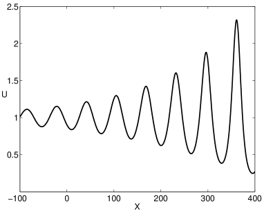
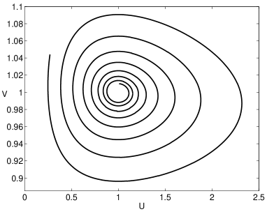
Figure 3.1: Oscillatory behavior of $U$ (left) and phase plane for $U,V$ (right).

3.3 The ODE regime

The key idea in computing the asymptotics of the solutions of (3.6)-(3.8) is to obtain suitable approximations of the operator $I\left[H\right]\left(X\right)$ in (3.8) for small $\lambda$. The formula for $H_{\lambda}$ (cf. (2.4)), combined with (2.5) and (3.8), suggests the approximation

$$I\left[H\right]\left(X\right)=\lambda\int_{-\infty}^{X}e^{\left(Y-X\right)}H\left(Y\right)dY\int_{\log\left(e^{X}-e^{Y}\right)}^{X}H\left(Z\right)dZ\,.$$ (3.12)

We will discuss the consistency of this assumption in Section 7.

The operator $I\left[H\right]\left(X\right)$ can be further approximated if $Y/X$ changes significantly faster than $H(Y)/H(X)$, as we saw is the case for $X\to-\infty$. Then it is natural to approximate $H(Y)$ by $H(X)$ and we obtain

$$I\left[H\right]\left(X\right)\sim\lambda H\left(X\right)\int_{-\infty}^{X}e^{\left(Y-X\right)}dY\int_{\log\left(e^{X}-e^{Y}\right)}^{X}H\left(Z\right)dZ\ \$$

and changing the order of the integrals

$$I\left[H\right]\left(X\right)\sim\lambda H\left(X\right)\int_{-\infty}^{X}H\left(Z\right)e^{Z-X}dZ\,.$$ (3.13)

From (3.7) we have

$$U\left(X\right)=\left(1{-}\lambda\right)\int_{-\infty}^{X}H\left(Z\right)e^{\left(1{-}\lambda\right)\left(Z-X\right)}dZ\sim\int_{-\infty}^{X}H\left(Z\right)e^{\left(Z-X\right)}dZ$$

which together with (3.13) leads to

$$I\left[H\right]\sim\lambda HU\,.$$ (3.14)

Using (3.14) as well as (2.4) and (2.5) we obtain the following approximation of (3.6) up to order $\lambda$:

$$H=UV+\lambda UV\left(U-1\right)$$ (3.15)

and plugging this approximation into (3.7), (3.8) we obtain

$$\frac{dU}{dX} =-\left(1{-}\lambda\right)U+\left(1{-}\lambda\right)UV+\lambda\left(1{-}\lambda\right)UV\left(U-1\right)\,,$$ (3.16)

$$\frac{dV}{dX} =\lambda V-\lambda UV-\lambda^{2}UV\left(U-1\right)\,.$$ (3.17)

As (3.2) and (3.11) imply that the changes of $\left(V{-}1\right)$ compared to those of $\left(U{-}1\right)$ are of order $\sqrt{\lambda}$, we make the change of variables

$$V=1+\sqrt{\lambda}\omega\ \ ,\ \ \xi=\sqrt{\lambda}X\,,$$ (3.18)

that transform (3.16), (3.17) up to order $\sqrt{\lambda}$ into

$$\frac{dU}{d\xi}=U\omega+\sqrt{\lambda}U\left(U-1\right)\ ,\ \ \ \ \frac{d\omega}{d\xi}=1-U+\sqrt{\lambda}\omega\left(1-U\right)\,.$$ (3.19)

3.4 Analysis of the ODE (3.19)

Let us denote by $\left(U_{\lambda},\omega_{\lambda}\right)$ any solution of (3.19). We first notice that the asymptotics of the solutions of (3.19) as $\left(U_{\lambda},\omega_{\lambda}\right)\rightarrow\left(1,0\right)$ agree with those obtained in (3.11). Indeed, in the limit $\lambda\rightarrow 0,$ we can compute the asymptotics of $\left(U,\omega\right)$ as $\xi\rightarrow-\infty$ using (3.11), (3.2) and (3.18):

$$\left((U_{\lambda}{-}1)\left(\xi\right),\omega_{\lambda}\left(\xi\right)\right)\sim\operatorname{Re}\left(K\left(1,i\right)e^{\left(i+O\left(\sqrt{\lambda}\right)\right)\xi}\right)\ \ \text{as}\ \ \xi\rightarrow-\infty\,.$$ (3.20)

Linearizing (3.19) near $\left(U,\omega\right)=\left(1,0\right)$ we obtain the same asymptotics for the functions $\left(U_{\lambda}\left(\xi\right),\omega_{\lambda}\left(\xi\right)\right)$ as $\xi\rightarrow-\infty.$ This gives the desired matching between the solutions of the linearization of (3.6)-(3.8) around $\left(H,U,V\right)=\left(1,1,1\right)$ and the solutions of the approximated problem (3.19).

The approximation (3.20) is valid as long as $\left|\left(U_{\lambda}-1\left(\xi\right),\omega_{\lambda}\left(\xi\right)\right)\right|$ is small. However, a detailed analysis of the nonlinear problem (3.19) is needed if $\left|\left(U_{\lambda}-1\left(\xi\right),\omega_{\lambda}\left(\xi\right)\right)\right|$ becomes of order one. In order to describe the solutions of (3.19) in this regime, we notice that this equation is a perturbation of the equation

$$\frac{dU_{0}}{d\xi}=U_{0}\omega_{0}\ ,\ \ \ \ \frac{d\omega_{0}}{d\xi}=1-U_{0}\,.$$ (3.21)

This equation can be explicitly integrated, since the following quantity is conserved along trajectories:

$$E=-\log\left(U_{0}\right)+\left(U_{0}-1\right)+\frac{\omega_{0}^{2}}{2}\,.$$ (3.22)

The solutions of (3.21) are periodic, but this behavior is not compatible with the exponential growth obtained in (3.20). This growth is due to the increase in $E$ produced by the terms of order $\sqrt{\lambda}$ in (3.19). We now compute this change of energy for values of $\left(U,\omega\right)$ of order one. Using (3.19) and (3.22) we obtain

$$\frac{dE}{d\xi}=\sqrt{\lambda}\left[\left(U_{\lambda}-1\right)^{2}+\omega_{\lambda}^{2}\left(1-U_{\lambda}\right)\right]\,.$$ (3.23)

Since the solutions of (3.19) are close to those of (3.21) during finite time intervals, we can adiabatically compute the change in $E.$ More precisely, the solutions of (3.21) satisfying (3.22) are periodic with a period $T\left(E\right)$ given by

$$T\left(E\right)=\sqrt{2}\int_{U_{-}\left(E,0\right)}^{U_{+}\left(E,0\right)}\frac{d\eta}{\eta\sqrt{E+\log\left(\eta\right)-\left(\eta-1\right)}}$$ (3.24)

where the functions $U_{-}\left(E,\omega\right)\leq U_{+}\left(E,\omega\right)$ are defined as the roots of the equation

$$\log\left(U\right)-\left(U-1\right)=\frac{\omega^{2}}{2}-E$$ (3.25)

for any given value of $\omega$ and $E\geq\frac{\omega^{2}}{2}.$ Integrating (3.23) and using the adiabatic approximation, we can then approximate the change of $E$ during an interval of length $T\left(E\right)$ as

$$\frac{E\left(T\left(E\right)\right)-E\left(0\right)}{\sqrt{\lambda}}=\int_{0}^{T\left(E\right)}\left[\left(U_{0}\left(\xi\right)-1\right)^{2}+\omega_{0}^{2}\left(\xi\right)\left(1-U_{0}\left(\xi\right)\right)\right]d\xi=\Phi\left(E\right)$$ (3.26)

where $\left(U_{0}\left(\xi\right),\omega_{0}\left(\xi\right)\right)$ is a solution of (3.21) satisfying (3.22).

It turns out that the function $\Phi\left(E\right)$ is positive for any $E>0.$ This follows, using the second equation in (3.21), via

$$\Phi\left(E\right)=\int_{-\sqrt{2E}}^{\sqrt{2E}}\left[\left(1-U_{-}\left(E,\omega\right)\right)+\omega^{2}\right]d\omega-\int_{-\sqrt{2E}}^{\sqrt{2E}}\left[\left(1-U_{+}\left(E,\omega\right)\right)+\omega^{2}\right]d\omega\,,$$

whence

$$\Phi\left(E\right)=2\int_{0}^{\sqrt{2E}}\left(U_{+}\left(E,\omega\right)-U_{-}\left(E,\omega\right)\right)d\omega>0\,.$$ (3.27)

We can compute the asymptotics of (3.27) as $E\rightarrow\infty$ using (3.25). Notice that the leading contribution to the integral is given by $U_{+}\left(E,\omega\right),$ since $U_{-}\left(E,\omega\right)\leq 1.$ Then

$$\Phi\left(E\right)\sim 2\int_{0}^{\sqrt{2E}}\left(E-\frac{\omega^{2}}{2}\right)d\omega=\frac{4\sqrt{2}}{3}E^{\frac{3}{2}}\ \ \text{as\ \ }E\rightarrow\infty\,.$$ (3.28)

3.5 Range of validity of the ODE regime

We have obtained that, as long as the approximation (3.19) is valid, we can approximate the functions $\left(U_{\lambda}\left(\xi\right),\omega_{\lambda}\left(\xi\right)\right)$ by $\left(U_{0}\left(\xi\right),\omega_{0}\left(\xi\right)\right)$ while $E$ is computed via the iterative recursion (3.26). Due to (3.28) these values of $E$ increase an amount of order $\sqrt{\lambda}\left(1+E\right)^{\frac{3}{2}}$ in each period of size $T\left(E\right).$ We now proceed to discuss the range of validity of the different approximations that have been used to derive (3.26) and (3.19).

To examine the range of values of $E$ for which the adiabatic approximation is valid, we need to show that the value of $E\left(\xi\right)$ remains close to $E\left(0\right)$ for $0\leq\xi\leq T\left(E\right).$ Due to (3.25) and (3.27) the adiabatic approximation is valid as long as

$$\sup_{0\leq\xi\leq T\left(E\right)}\left|E\left(\xi\right)-E\left(0\right)\right|\ll E\left(0\right)\,.$$ (3.29)

Let us remark that (3.29) does not follow immediately from the inequality $\left|E\left(T\left(E\left(0\right)\right)\right)-E\left(0\right)\right|\ll E\left(0\right)$ because the right-hand side of (3.23) does not have a sign and therefore it is not clear that

$$\sup_{0\leq\xi\leq T\left(E\right)}\left|E\left(\xi\right)-E\left(0\right)\right|\leq C\left|E\left(T\left(E\left(0\right)\right)\right)-E\left(0\right)\right|$$ (3.30)

for some $C>0.$ A priori it is not possible to rule out the possibility of big changes of $E\left(\xi\right)$ along each cycle balanced in such a way that the overall change of $E$ along the cycle is just $\Phi\left(E\right).$ However, as shown in Appendix A, it turns out that (3.30) holds true.

Using (3.26), (3.28) and (3.30) it follows that the adiabatic approximation is valid as long as $\sqrt{\lambda}\left(1+E\right)^{\frac{3}{2}}\ll\left(1+E\right)$ and this is satisfied as long as

$$\lambda\left(1+E\right)\ll 1\,.$$ (3.31)

We now study the range of validity of the approximation (3.14) that is the main ingredient in deriving the approximate problem (3.19). The main assumption used in the derivation of (3.14) is that the characteristic length scale for which $\left(H\left(X\right)-1\right)$ has changes comparable to itself is much larger than one. Due to (3.15) it follows that as long as $V$ remains close to $1$ the characteristic length scale for $\left(H-1\right)$ is the same as for $\left(U-1\right).$ Notice that $\left(V-1\right)$ is small if $\sqrt{\lambda}\omega\ll 1.$ Since we have $\frac{1}{2}\omega^{2}\leq E$, the condition $\sqrt{\lambda}\omega\ll 1$ holds if (3.31) is true, and so the characteristic length scales for $\left(H-1\right)$ and $\left(U-1\right)$ are the same under the assumption (3.31). For $\left|\left(U,\omega\right)\right|$ of order one, the evolution of (3.21) takes place in the length scale $\xi,$ or equivalently for changes in $X$ of order $\frac{1}{\sqrt{\lambda}}\gg 1.$ Therefore, the condition in (3.31) that allows us to obtain (3.14) is immediately satisfied and we can restrict our analysis to the case $\left|\left(U,\omega\right)\right|\gg 1.$ The first equation in (3.21) combined with (3.18) implies that

$$\left|\frac{d\left(\log\left(U\right)\right)}{dX}\right|=\sqrt{\lambda}\left|\omega\right|\,.$$ (3.32)

The left-hand side measures the relative variations in $U$ with respect to changes in $X.$ The characteristic length scale that describes the changes in this quantity is large as long as $\sqrt{\lambda}\left|\omega\right|\ll 1$ which is again true if (3.31) holds.

Therefore, if the condition (3.31) is satisfied, we can apply simultaneously all the approximations that lead to (3.19), the adiabatic approximation yielding (3.26) as well as the condition $\left|V-1\right|\ll 1.$ However, the three assumptions break down simultaneously if $E$ becomes of order $\frac{1}{\lambda}$. Since (3.26) and (3.28) imply that $E$ increases to arbitrarily large values, the failure of (3.31) happens for every solution of (3.6)-(3.8) satisfying (3.11).

4 The intermediate regime

In order to describe the solutions of (3.6)-(3.8) when $\lambda E\approx 1$ we introduce a new group of variables. It turns out to be convenient to split the regime into the one where $U$ (or $H$) is of order one or smaller, and the one where $U$ (or $H$) is large. Notice that (3.25) implies that for a given value of $E\sim\frac{1}{\lambda}$ the minimum of $U$ scales as $e^{-1/\lambda}$, and the maximum scales as $1/\lambda$. We remark that the forthcoming analysis will show that as long as $V$ remains of order one and is not small the values of $H$ and $U$ have the same order of magnitude. This assumption will be made implicitly in all the remaining computations and will be justified by the self-consistency of the derived asymptotics.

4.1 The integro-differential equation regime

We begin by studying the case in which $U$ (and $H$) are large. Since we are interested in the case $E\approx\frac{1}{\lambda}$, equation (3.25) suggests the rescaling $U\approx\frac{1}{\lambda},\ \omega\approx\frac{1}{\sqrt{\lambda}}.$ Then (3.32) yields a characteristic length scale for $X$ of order one. This suggests introducing the new set of variables

$$U\left(X\right)=\frac{1}{\lambda}\mathcal{U}\left(X\right),\ \ \ V\left(X\right)=\mathcal{V}\left(X\right),\ \ \ H\left(X\right)=\frac{1}{\lambda}\mathcal{H}\left(X\right)\,.\$$ (4.1)

Plugging (4.1) into (3.6)-(3.8) we obtain

$$\mathcal{H} =\frac{H_{\lambda}}{\lambda\left(1{-}\lambda\right)}\mathcal{U}\mathcal{V}+\frac{1}{\lambda}I\left[\mathcal{H}\right]\,,$$ (4.2)

$$\frac{d\mathcal{U}}{dX} =-\left(1{-}\lambda\right)\mathcal{U}+\left(1{-}\lambda\right)\mathcal{H}\,,\,\qquad\frac{d\mathcal{V}}{dX}=\lambda\mathcal{V}-\mathcal{H}\,,$$ (4.3)

where the operator $I\left[\mathcal{H}\right]$ is as in (3.8). Using the approximation (3.12) that will be seen to be still valid in this region we obtain

$$\frac{1}{\lambda}I\left[\mathcal{H}\right]\left(X\right)=\left(1+O\left(\lambda\right)\right)\int_{-\infty}^{X}e^{\left(Y-X\right)}\mathcal{H}\left(Y\right)dY\int_{\log\left(e^{X}-e^{Y}\right)}^{X}\mathcal{H}\left(Z\right)dZ\,.$$

Taking the limit $\lambda\rightarrow 0$ in (4.2)-(4.3) we obtain

$$\mathcal{H}\left(X\right) =\mathcal{U}\left(X\right)\mathcal{V}\left(X\right)+\int_{-\infty}^{X}e^{\left(Y-X\right)}\mathcal{H}\left(Y\right)dY\int_{\log\left(e^{X}-e^{Y}\right)}^{X}\mathcal{H}\left(Z\right)\,,dZ$$ (4.4)

$$\frac{d\mathcal{U}}{dX} =-\mathcal{U}+\mathcal{H}\ ,\ \ \ \frac{d\mathcal{V}}{dX}=-\mathcal{H}\,.$$ (4.5)

4.2 The ODE regime

If $\lambda E\approx 1$ but $U$ (and $H$) remains bounded we can approximate (3.6)-(3.8) as follows. Keeping just the leading terms in (3.6), (3.8) we arrive at the approximation $H=UV$. Plugging this approximation into (3.7) we obtain

$$\frac{dU}{dX}=-U+UV\ \ ,\ \ \ \ \frac{dV}{dX}=\lambda\left(V-UV\right)\,.$$ (4.6)

4.3 Explicit solution of (4.4), (4.5)

We are going to compute the solutions of (4.4), (4.5) explicitly using Laplace transforms. In order to bring (4.4), (4.5) into the form of a convolution equation we introduce the set of variables

$$x=e^{X}\ ,\ \ \mathcal{H}\left(X\right)=\bar{h}\left(x\right)\ ,\ \ \ \mathcal{U}\left(X\right)=\bar{u}\left(x\right)\ ,\ \ \mathcal{V}\left(X\right)=\bar{v}\left(x\right)$$ (4.7)

that transforms (4.4), (4.5) into

$$\bar{h}\left(x\right) =\bar{u}\left(x\right)\bar{v}\left(x\right)+\frac{1}{x}\int_{0}^{x}\bar{h}\left(y\right)dy\int_{x-y}^{x}\frac{\bar{h}\left(z\right)}{z}dz\,,$$ (4.8)

$$x\bar{u}_{x} =-\bar{u}+\bar{h}\ \ \ ,\ \ \ x\bar{v}_{x}=-\bar{h}\,.$$ (4.9)

Notice that this system of equations can be obtained from (2.8), (2.10) by means of the rescaling $h=\frac{\bar{h}}{\lambda},\ u=\frac{\bar{u}}{\lambda},\ v=\bar{v}$ and taking the limit $\lambda\rightarrow 0^{+}.$ We can compute explicitly a family of solutions of (4.8), (4.9) that will be used to describe the solutions of (3.6)-(3.8) in the limit $\lambda\rightarrow 0^{+}.$

Theorem 1

For any given $a\in(0,2)$ and $\kappa>0$ there exists a solution to (4.8), (4.9) that satifies

$$\bar{h}(0)=\bar{h}(\infty)=\bar{u}(0)=\bar{u}(\infty)=0\,,\ \ \lim_{x\rightarrow 0^{+}}\bar{v}\left(x\right)=1+a,\ \ \lim_{x\rightarrow\infty}\bar{v}\left(x\right)=1-a\,.$$ (4.10)

It is given by

$$\bar{v}\left(x\right)=\frac{1}{2\pi i}\int_{\gamma}\left[1+a\left(\frac{\zeta^{a}-\kappa x^{a}}{\zeta^{a}+\kappa x^{a}}\right)\right]\frac{e^{\zeta}}{\zeta}d\zeta$$ (4.11)

where $\gamma=\left\{\gamma\left(s\right):s\in\mathbb{R}\right\}$ is a contour in the complex plane contained in the domain $\left\{\arg\left(\zeta\right)\in\left(-\theta_{0},\theta_{0}\right)\right\}$ satisfying $\arg\left(\gamma\left(s\right)\right)\rightarrow-\theta_{0}$ as $s\rightarrow-\infty$ and $\arg\left(\gamma\left(s\right)\right)\rightarrow\theta_{0}$ as $s\rightarrow\infty$ with $\frac{\pi}{2}<\theta_{0}<\min\left\{\frac{\pi}{a},\pi\right\}.$

If $0<a<1$ we have $\bar{v}_{x}\left(x\right)<0,\ \bar{h}\left(x\right)>0$ and $\ \bar{u}\left(x\right)>0$ for any $x\in\mathbb{R}^{+}.$

The following asymptotics hold:

$$\bar{v}_{x}\left(x\right) \sim-\frac{2a\kappa}{\Gamma\left(a\right)}\frac{1}{x^{1-a}}\ \ \ \ \text{as\ \ }x\rightarrow 0^{+}\ \ ,\ \ a\in\left(0,2\right)$$ (4.12)

$$\bar{v}_{x}\left(x\right) \sim\frac{2a}{\kappa\Gamma\left(-a\right)}\frac{1}{x^{a+1}}\ \ \ \ \text{as\ \ }x\rightarrow\infty\ \ \ ,\ \ a\in\left(0,1\right)\cup\left(1,2\right)$$

$$\bar{h}\left(x\right) \sim\frac{2a\kappa}{\Gamma\left(a\right)}x^{a}\ \ \ \ \text{as\ \ }x\rightarrow 0^{+}\ \ \ \ ,\ \ a\in\left(0,2\right)$$ (4.13)

$$\bar{h}\left(x\right) \sim-\frac{2a}{\kappa\Gamma\left(-a\right)}\frac{1}{x^{a}}\ \ \ \ \text{as\ \ }x\rightarrow\infty\ \ \ ,\ \ a\in\left(0,1\right)\cup\left(1,2\right)$$

$$\bar{u}\left(x\right) \sim\frac{2a\kappa}{\Gamma\left(a\right)\left(a+1\right)}x^{a}\ \ \ \ \text{as\ \ }x\rightarrow 0^{+}\ \ \ \ ,\ \ a\in\left(0,2\right)$$ (4.14)

$$\bar{u}\left(x\right) \sim-\frac{2a}{\kappa\Gamma\left(-a\right)\left(1-a\right)}\frac{1}{x^{a}}\ \ \ \ \text{as\ \ }x\rightarrow\infty\ \ \ ,\ \ a\in\left(0,1\right)$$

If $a=1:$

$$\bar{v}\left(x\right)=2e^{-\kappa x}\ \ ,\ \ \bar{h}\left(x\right)=2\left(\kappa x\right)e^{-\kappa x}\ \ ,\ \ \bar{u}\left(x\right)=\frac{2}{\kappa x}\left(1-\left(1+\kappa x\right)e^{-\kappa x}\right)$$ (4.15)

Remark 2

The solutions with different values of $\kappa$ are essentially the same up to rescaling. Notice also that (4.10) implies that $\bar{v}\left(x\right)$ becomes negative for $x$ sufficiently large if $a>1.$

Remark 3

Some comments about the choice of the range of values of $a$ are in order. We need the restriction $0<a<2$ to avoid the singular points $\left(-\kappa\right)^{\frac{1}{a}}$ crossing the imaginary axis. It would also be possible to include the value $a=1$ in the second formula of (4.12) and (4.13) since the right-hand side vanishes. However this would result in asymptotic formulas like $f\sim 0$ that do not have a precise meaning. Finally the constraint $a<1$ in the second formula of (4.14) is strictly needed, since the asymptotics of $\bar{u}\left(x\right)$ for $a>1$ is proportional to $\frac{1}{x}.$

Remark 4

It is interesting to note that the solutions described in Theorem 1 for $0<a<1$ are just the self-similar solutions with algebraic decay that have been obtained for the coagulation equation with constant kernel in [13]. This correspondence can be seen as follows. The solutions we obtained in Theorem 1 satisfy

$$\bar{v}\left(x\right)=\left(1-a\right)+\int_{x}^{\infty}\bar{g}\left(z\right)dz\ \ ,\ \ \bar{u}\left(x\right)=\frac{1}{x}\int_{0}^{x}y\bar{g}\left(y\right)dy$$

with $\bar{g}\left(x\right)=\frac{\bar{h}\left(x\right)}{x}.$ Using this formula to eliminate $\bar{u},\ \bar{v}$ from (4.8) we obtain

$$x^{2}\bar{g}\left(x\right)=\left(1-a\right)\int_{0}^{x}y\bar{g}\left(y\right)dy+\int_{0}^{x}y\bar{g}\left(y\right)dy\int_{x-y}^{\infty}\bar{g}\left(z\right)dz\,.$$ (4.16)

Differentiating (4.16) we obtain the equation that is satisfied by the self-similar solutions of

$$\partial_{\tau}F=Q\left[F\right]-\frac{\left(1-a\right)}{\tau}F$$ (4.17)

having the form $f\left(\xi,\tau\right)=\frac{1}{\tau^{2}}\bar{g}\left(\frac{\xi}{\tau}\right)$ with $Q\left[\cdot\right]$ as in (1.1). Equation (4.17) can be transformed into (1.1) using the change of variables $F\left(\xi,\tau\right)=\left(\tau\right)^{-\left(1-a\right)}f\left(\xi,t\right)$ and $t=\frac{\tau^{a}}{a}$ and correspondingly the solutions obtained in Theorem 1 are transformed into those obtained in [13] if $0<a\leq 1.$

Proof. Integrating the first equation in (4.9) we arrive at

$$\bar{u}\left(x\right)=\frac{1}{x}\int_{0}^{x}\bar{h}\left(z\right)dz\,.$$ (4.18)

Using the second equation in (4.9) we obtain

$$\int_{x-y}^{x}\frac{\bar{h}\left(z\right)}{z}dz =-\bar{v}\left(x\right)+\bar{v}\left(x-y\right)\,,$$ (4.19)

$$\int_{0}^{x}\bar{h}\left(z\right)dz =-\int_{0}^{x}z\bar{v}_{z}\left(z\right)=-x\bar{v}\left(x\right)+\int_{0}^{x}\bar{v}\left(z\right)dz\,,$$ (4.20)

assuming that all the integrals involved are convergent. Therefore, using (4.18) and (4.20) we find

$$\bar{u}\left(x\right)=-\bar{v}\left(x\right)+\frac{1}{x}\int_{0}^{x}\bar{v}\left(z\right)dz\,.$$ (4.21)

Eliminating $\bar{h}$ and $\bar{u}$ from (4.8), the second equation in (4.9), as well as (4.18), (4.19), (4.20), implies

$$\begin{split}-x\bar{v}_{x}\left(x\right)&=-\left(\bar{v}\left(x\right)\right)^{2}+\frac{\bar{v}\left(x\right)}{x}\int_{0}^{x}\bar{v}\left(z\right)dz\\ &\quad-\frac{1}{x}\int_{0}^{x}y\bar{v}_{y}\left(y\right)\bar{v}\left(x-y\right)dy+\frac{\bar{v}\left(x\right)}{x}\int_{0}^{x}y\bar{v}_{y}\left(y\right)dy.\end{split}$$

Integrating by parts in the last equation we obtain

$$x^{2}\bar{v}_{x}\left(x\right)=\int_{0}^{x}y\bar{v}_{y}\left(y\right)\bar{v}\left(x-y\right)dy\,.$$ (4.22)

Equation (4.22) is a convolution equation. In order to solve it we introduce the Laplace transform of $\bar{v}\left(x\right)$

$$w\left(\zeta\right)=\int_{0}^{\infty}\bar{v}\left(x\right)e^{-\zeta x}dx\,.$$ (4.23)

Then (4.22) becomes $\frac{d^{2}}{d\zeta^{2}}\big{(}\zeta w\big{)}+w\frac{d}{d\zeta}\big{(}\zeta w\big{)}=0$. This equation can be integrated explicitly. Its only solution that does not have singularities and takes real values along the line $\zeta\in\mathbb{R}^{+}$ is

$$w\left(\zeta\right)=\frac{1}{\zeta}\left[1+a\left(\frac{\zeta^{a}-\kappa}{\zeta^{a}+\kappa}\right)\right]\,.$$ (4.24)

Inverting the Laplace transform we obtain

$$\bar{v}\left(x\right)=\frac{1}{2\pi i}\int_{\gamma}\left[1+a\left(\frac{\zeta^{a}-\kappa}{\zeta^{a}+\kappa}\right)\right]\frac{e^{\zeta x}}{\zeta}d\zeta\,.$$ (4.25)

The change of variables $\zeta x=\hat{\zeta}$ transforms this formula into (4.11). The choice of the contour of integration ensures the exponential convergence of the integral as well as the absence of singularities of the integrand along the contour of integration. Taking the limits $x\rightarrow 0^{+}$ and $x\rightarrow\infty$ we obtain (4.10).

The negativity of $\bar{v}_{x}$ for $0<a<1$ can be proved by differentiating (4.25) and deforming the contour of integration to a double half-line following $\mathbb{R}^{-}$ in a positive and negative direction with $\arg\left(\zeta\right)=-\pi$ and $\arg\left(\zeta\right)=\pi$ respectively. Then

$$\bar{v}_{x}\left(x\right)=-\frac{2a\kappa\sin\left(a\pi\right)}{\pi}\int_{0}^{\infty}\frac{e^{-rx}r^{a}dr}{\left|\kappa+e^{a\pi i}r^{a}\right|^{2}}\ \ ,\ \ 0<a<1\,.$$

The asymptotics in (4.12) can be obtained rewriting (4.25) as

$$\bar{v}\left(x\right)=\left(1+a\right)-\frac{\kappa a}{\pi i}\int_{\gamma}\left(\frac{1}{\zeta^{a}+\kappa}\right)\frac{e^{\zeta x}}{\zeta}d\zeta$$

and

$$\bar{v}\left(x\right)=\left(1-a\right)+\frac{a}{\pi i}\int_{\gamma}\left(\frac{\zeta^{a}}{\zeta^{a}+\kappa}\right)\frac{e^{\zeta x}}{\zeta}d\zeta\,.$$

Differentiating these formulas we obtain

$$\bar{v}_{x}\left(x\right)=-\frac{\kappa a}{\pi i}\int_{\gamma}\frac{e^{\zeta x}}{\zeta^{a}+\kappa}d\zeta\ \ ,\ \ \bar{v}_{x}\left(x\right)=\frac{a}{\pi i}\int_{\gamma}\left(\frac{\zeta^{a}}{\zeta^{a}+\kappa}\right)e^{\zeta x}d\zeta$$

and using the change of variables $\zeta x=\hat{\zeta}$ in both integrals it follows that

$$\bar{v}_{x}\left(x\right)=-\frac{\kappa a}{\pi i}\frac{1}{x^{1-a}}\int_{\gamma}\frac{e^{\zeta}}{\zeta^{a}+\kappa x^{a}}d\zeta\ \ ,\ \ \bar{v}_{x}\left(x\right)=\frac{a}{\pi i}\frac{1}{x}\int_{\gamma}\left(\frac{\zeta^{a}}{\zeta^{a}+\kappa x^{a}}\right)e^{\zeta}d\zeta\,.$$

Taking the limit $x\rightarrow 0^{+}$ in the first formula and $x\rightarrow\infty$ in the second and using the fact that

$$\frac{1}{\pi i}\int_{\gamma}\frac{e^{\zeta}}{\zeta^{a}}d\zeta=\frac{2}{\Gamma\left(a\right)}\ \ \ \ \ ,\ \ \ \ \frac{1}{\pi i}\int_{\gamma}\zeta^{a}e^{\zeta}d\zeta=\frac{2}{\Gamma\left(-a\right)}$$

we obtain (4.12). Using then (4.9) we obtain (4.13), (4.14).

Formula (4.15) follows by integrating by residues.   

We can reformulate the results in Theorem 1 in terms of the original functions $\left(\mathcal{H}\left(X\right),\mathcal{U}\left(X\right),\mathcal{V}\left(X\right)\right).$ In the following we choose $\kappa=1$ as a suitable normalization.

Theorem 5

For any $0<a<2$ there exists a solution of (4.4), (4.5) satisfying $\mathcal{H}(-\infty)=\mathcal{H}(\infty)=\mathcal{U}(-\infty)=\mathcal{U}(\infty)=0$. It is given by

$$\mathcal{V}_{a}\left(X\right)-1=\frac{a}{2\pi i}\int_{\gamma}\left(\frac{\zeta^{a}-e^{aX}}{\zeta^{a}+e^{aX}}\right)\frac{e^{\zeta}}{\zeta}d\zeta$$ (4.26)

$$\mathcal{H}_{a}\left(X\right)=-\frac{d\mathcal{V}_{a}\left(X\right)}{dX}\ \ ,\ \ \mathcal{U}_{a}\left(X\right)=-\int_{-\infty}^{X}e^{\left(Z-X\right)}\frac{d\mathcal{V}_{a}\left(Z\right)}{dZ}dZ$$ (4.27)

$$\lim_{X\rightarrow-\infty}\mathcal{V}_{a}\left(X\right)=1+a\ \ \ ,\ \ \ \lim_{X\rightarrow\infty}\mathcal{V}_{a}\left(X\right)=1-a\,.$$ (4.28)

If $0<a<1$ we have $\frac{d\mathcal{V}_{a}\left(X\right)}{dX}<0,\ \mathcal{H}_{a}\left(X\right)>0,\ \mathcal{U}_{a}\left(X\right)>0$ for any $X\in\mathbb{R}$. We have the asymptotics

$$\frac{d\mathcal{V}_{a}\left(X\right)}{dX} \sim-\frac{2a}{\Gamma\left(a\right)}e^{aX}\ \ \text{as\ \ }X\rightarrow-\infty,\ \ a\in\left(0,2\right)$$ (4.29)

$$\frac{d\mathcal{V}_{a}\left(X\right)}{dX} \sim\frac{2a}{\Gamma\left(-a\right)}e^{-aX}\ \ \text{as\ \ }X\rightarrow\infty\ \ \ ,\ \ a\in\left(0,1\right)\cup\left(1,2\right)$$

$$\mathcal{H}_{a}\left(X\right) \sim\frac{2a}{\Gamma\left(a\right)}e^{aX}\ \ \ \ \text{as\ \ }X\rightarrow-\infty\ \ \ \ ,\ \ a\in\left(0,2\right)$$ (4.30)

$$\mathcal{H}_{a}\left(X\right) \sim-\frac{2a}{\Gamma\left(-a\right)}e^{-aX}\ \ \ \ \text{as\ \ }X\rightarrow\infty\ \ \ ,\ \ a\in\left(0,1\right)\cup\left(1,2\right)$$

$$\mathcal{U}_{a}\left(X\right) \sim\frac{2a}{\Gamma\left(a\right)\left(a+1\right)}e^{aX}\ \ \ \ \text{as\ \ }X\rightarrow-\infty\ \ \ \ ,\ \ a\in\left(0,2\right)$$ (4.31)

$$\mathcal{U}_{a}\left(X\right) \sim-\frac{2a}{\Gamma\left(-a\right)\left(1-a\right)}e^{-aX}\ \ \ \ \text{as\ \ }X\rightarrow\infty\ \ \ ,\ \ a\in\left(0,1\right)$$

If $a=1:$

$$\mathcal{V}_{a}\left(X\right)=2e^{-e^{X}},\,\mathcal{H}_{a}\left(X\right)=2e^{X}e^{-e^{X}},\,\mathcal{U}_{a}\left(X\right)=2e^{-X}\left(1-\left(1+\kappa e^{X}\right)e^{-e^{X}}\right)$$ (4.32)

4.4 Solution of (4.6)

Equation (4.6) that approximates the behaviour of the solutions of (3.6)-(3.8) if $\lambda E\approx 1$ and $U$ is of order one, can be solved explicitly since

$$\hat{E}=\lambda\left(\log\left(U\right)-U\right)-V+\log\left(V\right)$$ (4.33)

is preserved along trajectories. The solutions of (4.6) will be used to match the solutions of (4.4), (4.5) obtained in the previous Section for $1\ll U\ll\frac{1}{\lambda}.$ For this range of values $V$ is almost constant if $\lambda\rightarrow 0.$ Moreover, since we are away from the ODE regime described in Section 3.4 we can assume that $\lambda E$ in (3.25) is of order one and therefore $\hat{E}$ is of order one, whence also $\left|V-1\right|$ is of order one.

Suppose that we consider a matching region (to be made precise later) where $\hat{E}$ is of order one, $V$ is almost constant and satisfies $V<1$. Then the first equation in (4.6) implies that $U$ decreases exponentially. More preciesely, let us assume that $U=1$ for $X=X^{-}.$ Then, the asymptotics of $U,\ V$ are

$$V\sim\left(1-a^{-}\right)\ \ ,\ \ \ \ U\sim\exp\left(-a_{-}\left(X-X^{-}\right)\right)$$ (4.34)

for some $a^{-}\in\left(0,1\right)$. The asymptotics (4.34) will be shown to match with suitable solutions among the ones described in Theorem 1. Moreover, notice that (4.6) implies that these asymptotics are valid as long as $U$ remains larger than some small number $\varepsilon_{0}$ that we can assume to be of order one, although small. The exponential decay of $U$ in (4.34) implies that the transition between $U=1$ and $U=\varepsilon_{0}$ takes place on a length scale $\left(X-X^{-}\right)$ of order one.

We now describe the solution when $U$ is less than $\varepsilon_{0}$. For this purpose let us define by $a_{-}$ and $a_{+}$ the two roots of the equation $\hat{E}=-V+\log\left(V\right)$. Then, in the limit $\lambda\rightarrow 0^{+}$, the curves given by (4.33) in the plane $\left(U,V\right)$ are approximately the two horizontal lines $\left\{V=1-a_{-}\right\}$ and $\left\{V=1+a_{+}\right\}$ connected by a curve that is approximately vertical. Along this connecting curve $V$ changes an amount of order one and $\lambda\log\left(U\right)$ continues to be of order one since $\hat{E}$ is preserved. When $U$ is less than $\varepsilon_{0}$ we can approximate the second equation in (4.6) as $\frac{dV}{dX}=\lambda\left(1+O\left(\varepsilon_{0}\right)\right)V.$ Then $V\left(X\right)$ increases exponentially. The first equation in (4.6) indicates that for the solutions of (4.6) under consideration, $U$ remains small while $V$ changes from $\left(1-a_{-}\right)$ to$\ \left(1+a_{+}\right).$ Then we can use the approximation

$$V=\left(1-a_{-}\right)\exp\left(\lambda\left(1+O\left(\varepsilon_{0}\right)\right)\left(X-X^{-}-\ell_{trans}^{-}\right)\right)$$ (4.35)

where $\ell_{trans}^{-}$ is the range of $X$ that it takes for $U$ to decrease from $U=1$ to $U=\varepsilon_{0}.$ We recall that $\ell_{trans}^{-}$ is of order one.

Notice that the structure of the curve (4.33) implies that eventually $U$ becomes again of order $\varepsilon_{0}$ with $V$ close to $\left(1+a_{+}\right).$ It then follows from (4.6) that for small $\lambda,$ $U$ reaches again the value $1$ at $X^{+}$ after an additional length $\ell_{trans}^{+}$ of order one. Notice that, using (4.35), we have

$$V=\left(1-a_{-}\right)\exp\left(\lambda\left(1+O\left(\varepsilon_{0}\right)\right)\left(X^{+}-X^{-}-\ell_{trans}^{+}-\ell_{trans}^{-}\right)\right)$$ (4.36)

and $U$ has the behaviour, for $\varepsilon_{0}\leq U\ll\frac{1}{\lambda}$,

$$U\sim\exp\left(a_{+}\left(X-X^{+}\right)\right)\,.$$ (4.37)

We need to estimate the relation between $a_{-}$ and $a_{+}.$ From (4.33) we deduce that to leading order

$$\log\left(1-a_{-}\right)+a_{-}=\log\left(1+a_{+}\right)-a_{+}\,.$$ (4.38)

On the other hand (4.36) allows us to obtain an approximation for the transition length $\left(X^{+}-X^{-}\right).$ Indeed, we have

$$\left(1+a_{+}\right)=\left(1-a_{-}\right)\exp\left(\lambda\left(1+O\left(\varepsilon_{0}\right)\right)\left(X^{+}-X^{-}-\ell_{trans}^{+}-\ell_{trans}^{-}\right)\right)$$

whence, since $\ell_{trans}^{+},\ \ell_{trans}^{-}$ are of order one and $\varepsilon_{0}$ can be made arbitrarily small

$$\left(X^{+}-X^{-}\right)\sim\frac{1}{\lambda}\log\left(\frac{1+a_{+}}{1-a_{-}}\right)$$ (4.39)

as $\lambda\rightarrow 0^{+}.$

We have described the transition of the solution $\left(U,V,H\right)$ of (3.6)-(3.8) for small $\lambda$ and $U\ll\frac{1}{\lambda}.$ The following result will play a crucial role in describing the solutions, because it will show that the amplitude of the oscillations increases with $X.$

Lemma 6

Suppose that $a_{-}>0,$ $a_{+}>0$ satisfy (4.38). Then $a_{+}>a_{-}$.

Proof. This follows from the inequality $\log\left(1+x\right)-x>\log\left(1-x\right)+x$ that is just a consequence of $\log\left(1+x\right)-\log\left(1-x\right)=\int_{0}^{x}\frac{2dr}{\left(1-r^{2}\right)}>2x$.   

4.5 Coupling of the regimes

4.5.1 Description of the iterative procedure

We now describe the behaviour of the solutions of (3.6)-(3.8) for $\lambda\rightarrow 0$ and $\lambda E\approx 1,$ with $E$ as in (3.25). It turns out that these solutions can be described for this range of values by a sequence of intervals where the solutions can be approximated alternately by solutions of (4.4), (4.5) or by solutions of (4.6) with both types of regions connected with suitable matching regions.

More precisely, suppose that $X_{n}^{+}$ is a point where $U\left(X_{n}^{+}\right)=1\ ,\ \ V\left(X_{n}^{+}\right)=1+a_{n}$. Notice that at such a point we can expect to be able to use the approximation (4.6). This will be seen matching the ODE-Integrodifferential equation regime with the ODE regime described in Section 3.3. We will assume for the moment that this approximation is valid. Then $H$ is also of order one and we can approximate it to the leading order as $H=UV$ (cf. Section 4.2). We can also use the approximation (4.37) with $a_{+}=a_{n}$ and approximate $V$ by a constant. Then we obtain for $\left|X-X_{n}^{+}\right|$ of order one that

$$U\sim\exp\left(a_{n}\left(X-X_{n}^{+}\right)\right)\ \ ,\ \ V\sim 1+a_{n}\ \ ,\ \ H\sim\left(1+a_{n}\right)\exp\left(a_{n}\left(X-X_{n}^{+}\right)\right)\,.$$ (4.40)

We can now match the asymptotics (4.40) with those obtained for the solutions of (4.4), (4.5). We use (4.1) to obtain the matching condition

$$\begin{split}\mathcal{U}\left(X\right)\sim\lambda\exp\left(a_{n}\left(X-X_{n}^{+}\right)\right)\ &,\ \ \mathcal{V}\left(X\right)\sim\left(1+a_{n}\right)\,,\\ \mathcal{H}\left(X\right)&\sim\lambda\left(1+a_{n}\right)\exp\left(a_{n}\left(X-X_{n}^{+}\right)\right)\,.\end{split}$$ (4.41)

This behaviour must be matched with the one for the solutions of (4.4), (4.5) obtained in Theorem 5. More precisely we will match these behaviours with the ones of

$$\Phi_{n}\left(X\right)=\left(\mathcal{U}_{a_{n}}\left(X-X_{n}^{0}\right),\mathcal{V}_{a_{n}}\left(X-X_{n}^{0}\right),\mathcal{H}_{a_{n}}\left(X-X_{n}^{0}\right)\right)$$

for a suitable choice of $a_{n}$ and $X_{n}^{0}.$ The asymptotics of $\mathcal{V}\left(X\right)$ combined with the one in (4.28) yield $a=a_{n},$ since in the matching region we expect to have $\left(X-X_{n}^{0}\right)\rightarrow-\infty.$ On the other hand (4.30), (4.31) give the choice

$$X_{n}^{0}=X_{n}^{+}+\frac{1}{a_{n}}\log\left(\frac{2a_{n}}{\left(1+a_{n}\right)\Gamma\left(a_{n}\right)}\frac{1}{\lambda}\right)\,.$$ (4.42)

With these choices of $a_{n}$ and $X_{n}^{0}$ we obtain, using (4.28), (4.30), (4.31) and (4.41), a matching to the first order between (4.40) and $\Phi_{n}\left(X\right)$ in the common region of validity where $\left(X-X_{n}^{+}\right)\gg 1$ and $\left(X-X_{n}^{0}\right)\ll 1$.

We can then use the approximation $\Phi_{n}\left(X\right)$ to describe the solutions of (3.6)-(3.8) for small $\lambda$ and $\left(X-X_{n}^{0}\right)$ of order one. This approximation breaks down for $\left(X-X_{n}^{0}\right)$ sufficiently large. Indeed, (4.30) and (4.31) imply that $\mathcal{U}_{a}\left(X-X_{n}^{0}\right)$ and $\mathcal{H}_{a}\left(X-X_{n}^{0}\right)$ converge exponentially to zero as $\left(X-X_{n}^{0}\right)\rightarrow\infty.$ However, the approximation (4.4), (4.5) is only valid if $\left|\left(\mathcal{U}\left(X\right),\mathcal{H}\left(X\right)\right)\right|\gg\lambda.$ In the region where $\left|\left(\mathcal{U}\left(X\right),\mathcal{H}\left(X\right)\right)\right|$ becomes of order $\lambda$ we must use again the approximation (4.6). In particular this region can be described using the analysis in Section 4.4. The asymptotics of the solutions for $U$ of order one is as in (4.34) for suitable choices of $a_{-},\ X^{-}.$ More precisely, since this matching is made for $\left(X-X_{n}^{0}\right)\gg 1$ we can use the asymptotics (4.28), (4.30), (4.31) for $X\rightarrow\infty.$ We then obtain, using also the rescaling (4.1), the matching conditions

$$\begin{split}U\left(X\right)\sim-\frac{2a_{n}}{\Gamma\left(-a_{n}\right)\left(1-a_{n}\right)\lambda}e^{-a_{n}\left(X-X_{n}^{0}\right)}\ ,&\ \ \ V\left(X\right)\sim\left(1-a_{n}\right)\\ H\left(X\right)\sim-\frac{2a_{n}}{\Gamma\left(-a_{n}\right)\lambda}e^{-a_{n}\left(X-X_{n}^{0}\right)}&\qquad\mbox{ for }\left(X-X_{n}^{0}\right)\gg 1,\ \ U\gg 1\,.\end{split}$$

We now match these formulas with (4.34) (combined with the approximation $H=UV$). To this end we must choose

$$a_{-}=a_{n}\ ,\ \ \ X_{n}^{-}=X_{n}^{0}+\frac{1}{a_{n}}\log\left(-\frac{2a_{n}}{\left(1-a_{n}\right)\Gamma\left(-a_{n}\right)}\frac{1}{\lambda}\right)\,.$$ (4.43)

We remark that all this analysis will be meaningful only if $0<a_{n}<1.$ Therefore $\Gamma\left(-a_{n}\right)<0.$

The region where $U\leq 1,\ H\leq 1$ can then be described using the analysis in Section 4.4. The conclusion of this analysis is that $\left(U,V\right)$ moves close to the point $\left(1,\left(1+a_{n+1}\right)\right)$ for some suitable $a_{n+1}$ in a characteristic length given by (4.39). More precisely if we define (cf. (4.38))

$$\log\left(1-a_{n}\right)+a_{n}=\log\left(1+a_{n+1}\right)-a_{n+1}\ \ ,\ \ a_{n}>0\ \ ,\ \ a_{n+1}>0$$ (4.44)

$$X_{n+1}^{+}=X_{n}^{-}+\frac{1}{\lambda}\log\left(\frac{1+a_{n+1}}{1-a_{n}}\right)$$ (4.45)

we can approximate $U,\ V$ by means of (4.40) with $X_{n}^{+}$ replaced by $X_{n+1}^{+}.$

Combining (4.42), (4.43) and (4.45) we obtain to the leading order

$$X_{n+1}^{+}-X_{n}^{+}\sim\frac{1}{\lambda}\log\left(\frac{1+a_{n+1}}{1-a_{n}}\right)\,.$$ (4.46)

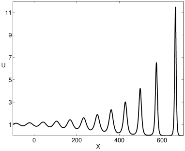
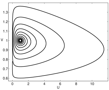
Figure 4.1: Intermediate regime: $U$ (left) and phase plane for $U,V$ (right)

4.5.2 Matching with the ODE regime

We first remark that equation (3.19) agrees with the approximating equations (4.4), (4.5) and (4.6) if $E\gg 1,\ E\ll\frac{1}{\lambda}$ in their respective regimes of validity.

Indeed, we can rewrite (3.19) using (3.18) as

$$\frac{dU}{dX}=U\left(V-1\right)+\lambda U\left(U-1\right)\ \ \ ,\ \ \ \frac{dV}{dX}=\lambda\left(1-U\right)V$$ (4.47)

and these equations yield the same behaviour as (4.6) if $U$ is bounded.

On the other hand, in order to approximate the solutions of (4.4), (4.5) for $E\gg 1,\ E\ll\frac{1}{\lambda}$ we use the fact that for small $a,$ the solutions of (4.4), (4.5) in Theorem 5 have the characteristic length scale $\frac{1}{a}.$ Then, for $a$ small, which corresponds to the matching region indicated above, we have a characteristic length very large compared with one. Then, as in (3.14) we can approximate $I\left[\mathcal{H}\right]\sim\lambda\mathcal{H}\mathcal{U}$. Since $E\ll\frac{1}{\lambda}$ we have $\mathcal{U}\left(X\right)\ll 1$ and we obtain from (4.4) the approximation $\mathcal{H}\left(X\right)=\mathcal{U}\left(X\right)\mathcal{V}\left(X\right)+\left(\mathcal{U}\left(X\right)\right)^{2}\mathcal{V}\left(X\right)$ and plugging this formula into (4.5) and using the rescaling (4.1) we obtain

$$\frac{dU}{dX}=U\left(V-1\right)+\lambda\left(U\right)^{2}V\ \ ,\ \ \frac{dV}{dX}=-\lambda UV-\lambda^{2}\left(U\right)^{2}V$$

that agrees with (4.47) in the range of values $U\gg 1,\ U\ll\frac{1}{\lambda}.$

The previous computations show that the equations used in both transition regimes agree in the intermediate matching regime. Actually it is possible to check that the main characteristics of the computed solution also agree, as could be expected. Notice that the length scale $\left(X_{n+1}^{+}-X_{n}^{+}\right)$ can be computed using the function $T\left(E\right)$ in (3.24) for $E\gg 1,\ E\ll\frac{1}{\lambda}$:

$$T\left(E\right)\sim 2\sqrt{2}\sqrt{E}\,.\$$ (4.48)

In the computation of this integral, we have split the region of integration into the two subsets $\left(U_{-}\left(E,0\right),\varepsilon_{0}\right)$ and $\left(\varepsilon_{0},U_{+}\left(E,0\right)\right)$ where $\varepsilon_{0}>0$ is a small but fixed number. It turns out that the contribution of the second integral is much smaller than the one due to the first integrand, exactly in the same manner that the contributions in $\left(X_{n+1}^{+}-X_{n}^{+}\right)$ computed in Subsection 4.5.1 are due mostly to the region with small values of $U.$ Using the rescaling (3.18) we then obtain the approximation

$$\left(X_{n+1}^{+}-X_{n}^{+}\right)\sim\frac{2\sqrt{2}\sqrt{E}}{\sqrt{\lambda}}\,.$$ (4.49)

On the other hand, we can compute the same length using (4.46). Taking into account that in the matching region $a_{n},\ a_{n+1}$ are small, we obtain from (4.44) that

$$a_{n+1}\sim a_{n}+\frac{2}{3}\left(a_{n}\right)^{2}\,.$$ (4.50)

Using (4.46) we then obtain to leading order that

$$X_{n+1}^{+}-X_{n}^{+}\sim\frac{\left(a_{n}+a_{n+1}\right)}{\lambda}\sim\frac{2a_{n}}{\lambda}\,.$$ (4.51)

Next, equation (3.25) and the definition of $a_{n}$ by means of $U=1,$ imply

$$a_{n}=\sqrt{2}\sqrt{E}\sqrt{\lambda}$$ (4.52)

and plugging (4.52) into (4.51) we obtain the sought-for matching with (4.49).

Finally we obtain the matching for the formula of the change of energy in each iteration. We have obtained using the ODE approximation that the change of energy in each cycle is given by (3.26) where in the matching region $1\ll E\ll\frac{1}{\lambda}$ we can use the approximation (3.28). Then

$$E_{n+1}-E_{n}\sim\frac{4\sqrt{2}}{3}E_{n}^{\frac{3}{2}}\,.$$ (4.53)

On the other hand, using again $a_{n}=\sqrt{2}\sqrt{E}\sqrt{\lambda}$ and plugging it in (4.50) we obtain again (4.53) and this yields the desired matching.

5 Shooting argument

The structure of the solutions of (3.6)-(3.8) described in Section 4.5 by means of alternate approximate solutions of (4.4)-(4.5) and (4.6) yields several sequences of numbers $\left\{a_{n}\right\},\ \left\{X_{n}^{+}\right\},\ \left\{X_{n}^{-}\right\},\ \left\{X_{n}^{0}\right\}$ that measure the amplitude of the oscillations, the positions of the points where $U=1,\ V>1,\ U=1,\ V<1$ and the position of the peaks where $U$ and $H$ are of order $\frac{1}{\lambda}$ respectively. It is relevant to notice that the sequence $\left\{a_{n}\right\}$ is increasing due to Lemma 6. The values of $a_{n}$ approach zero in the matching region (see the approximation (4.52) for $1\ll E\ll\frac{1}{\lambda}$), but they become of order one for $E\approx\frac{1}{\lambda}$ with increases in each iteration of order one. Eventually, this sequence of points becomes larger than or equal to one.

A detailed study of the solutions of (3.6)-(3.8) shows that there are several possibilities. If $a_{n}$ becomes strictly larger than one, Theorem 5 shows that during the peak regime $V$ becomes strictly negative. In particular $V$ reaches the value $V=0$ at some finite $X_{\ast}.$ If $V$ remains positive for larger values of $X$, something that could happen if $a_{n}=1,$ it would be possible to approximate (3.6)-(3.8) by means of (4.6). Therefore $V$ would increase, and the value of $a_{n}$ would be increased to a new value $a_{n+1}>1$ at the next iteration. The only possibility of not having such a behaviour would be with $V\rightarrow 0$ as $X\rightarrow\infty.$ Such approximation to zero cannot be described by the approximate equation (4.6), because in such a regime the integral terms in (3.6)-(3.8) must be taken into account in full detail.

We now recall that for any $K\in\mathbb{C}$ there exists a unique solution of (3.6)-(3.8) satisfying (3.11). The discussion in Section 3.2 shows that all the solutions of (3.6)-(3.8) with such a behaviour can be obtained, up to rescaling, by choosing $K$ in the interval $\left[1,\exp\left(\frac{2\pi\beta\left(\lambda\right)}{\alpha\left(\lambda\right)}\right)\right).$ A continuity argument taking into account the behaviour of the trajectories shows that there exists a value of $K=K_{\ast}$ in this interval for which the corresponding solution of (3.6)-(3.8) satisfies $\lim_{X\rightarrow\infty}V\left(X\right)=0.$ This also implies $\lim_{X\rightarrow\infty}H\left(X\right)=0$ and $\lim_{X\rightarrow\infty}U\left(X\right)=0$ using (3.6), (3.7). More precisely, the inversion of (3.6) allows us to write $H\left(X\right)$ in terms of $UV.$ Then $\lim_{X\rightarrow\infty}H\left(X\right)=0$ and (3.7) yields $\lim_{X\rightarrow\infty}U\left(X\right)=0.$

6 Asymptotics as $X\rightarrow\infty$

We finally describe the asymptotics of the solution of (3.6)-(3.8) satisfying (3.11) with $K=K_{\ast}$ described in the previous Section. We have seen that $\lim_{X\rightarrow\infty}U\left(X\right)=\lim_{X\rightarrow\infty}V\left(X\right)=\lim_{X\rightarrow\infty}H\left(X\right)=0\,.$ To leading order the behaviour of this trajectory is described by the solution of (4.4), (4.5) given in Theorem 5 with $a=1.$ The asymptotics

$$H\left(X\right)\sim\frac{2e^{\left(X-X_{n}^{0}\right)}e^{-e^{\left(X-X_{n}^{0}\right)}}}{\lambda}$$ (6.1)

is valid as long as $H\gg 1,\ \left(X-X^{0}_{n}\right)\gg 1$, where, by assumption, to the leading order $a_{n}=1.$ It is convenient to reformulate (6.1) in the original variables (cf. (3.4), (3.5))

$$h\left(x\right)\sim\frac{2}{\lambda}\left(\frac{x}{x_{n}}\right)\exp\left(-\left(\frac{x}{x_{n}}\right)\right)$$ (6.2)

that is valid for $\frac{x}{x_{n}}\gg 1,\ h\gg 1.$

We can match (6.2) with the following exponential asymptotics for the solutions of (2.7) as $x\rightarrow\infty$:

$$h\left(x\right)\sim\frac{2}{\lambda}\left(\kappa x\right)\exp\left(-\kappa x\right)$$ (6.3)

The asymptotics (6.2), (6.3) match for small $\lambda$ if $\kappa=\frac{1}{x_{n}}.$ This gives the desired exponential decay for the obtained solution.

7 Self-consistency of the approximations of $I\left[H\right]$

We now show that the solution we obtained is self-consistent with the approximations made for the integral operator $I\left[H\right]\left(X\right)$ defined in (3.8). We have made two main approximations. The first one is (3.12), that approximates $I\left[H\right]$ by an operator with a simple dependence on $\lambda.$ The second approximation is (3.14) and it allows us to replace the integral operator by a much simpler local operator.

Concerning the validity of (3.12) we remark that its precise meaning is that the error made in the approximation is smaller than the right-hand side. In order to check its validity we distinguish between the regions where $H$ is of order $\frac{1}{\lambda}$ and the regions where $H$ is smaller than that quantity.

Notice that for any region we can expect the errors made in the approximation to be of order

$$R_{1} =\lambda^{2}\int_{-\infty}^{X}dYe^{\left(Y-X\right)}\left(X-Y\right)H\left(Y\right)\int_{\log\left(e^{X}-e^{Y}\right)}^{X}dZH\left(Z\right)\,,$$

$$R_{2} =\lambda^{2}\int_{-\infty}^{X}dYe^{\left(Y-X\right)}H\left(Y\right)\int_{\log\left(e^{X}-e^{Y}\right)}^{X}dZ\left(X-Z\right)H\left(Z\right)$$

and we can expect these two terms to be very small compared with the right-hand side of (3.12). Indeed, in the case of $R_{1}$, the contribution due to the region $\lambda\left(X-Y\right)\leq\varepsilon_{0}$ is small compared with the term in (3.12) if $\varepsilon_{0}$ is small. On the other hand, if $\lambda\left(X-Y\right)>\varepsilon_{0}$ we can use the smallness of the exponential factor $e^{\left(Y-X\right)}$ to obtain estimates for the corresponding terms in $R_{1}$ as $C\lambda^{2}\left\|H\right\|_{\infty}^{2}e^{-\frac{\varepsilon_{0}}{\lambda}}$ and since $\left\|H\right\|_{\infty}\leq C/\lambda$ it then follows that this contribution is exponentially small. Concerning $R_{2}$ we can argue similarly for $\lambda\left(X-Z\right)$ smaller than $\varepsilon_{0}$. If $\lambda\left(X-Z\right)>\varepsilon_{0}$, since $Z\geq X+\log\left(1-e^{Y-X}\right)$ it follows that the size of the region of integration can be bounded by $Ce^{-\frac{\varepsilon_{0}}{\lambda}}$ and therefore, it gives also a very small contribution.

Concerning the approximations of $I\left[H\right]$ by means of local terms that have been made in the derivation of the ODE approximations (3.19) or (4.6) two main ingredients are required. In the derivation of (3.19) we have used just the fact that $H\left(Y\right)$ has significant changes over distances much longer than one. Since the order of magnitude of $H$ is roughly the same for the range of values described by means of (3.19) no special care is required to estimate the values of $H\left(Y\right)$ with $X-Y\gg 1.$ On the other hand, in the case of the approximation (4.6) we use the fact that $I\left[H\right]$ is a corrective term that is completely ignored in (4.6). Notice that $H\left(Y\right)$ takes values for $Y<X$ much larger than the ones of $H\left(X\right)$ in the region where the approximation (4.6) is used. However, due to the exponential factor $e^{\left(Y-X\right)}$ as well as the exponential decay of $H\left(Y\right)$ in the region described by the integro-differential equation (cf. Subsection 4.5.1) the corresponding contribution of such values of $H\left(Y\right)$ is negligible.

Appendix A Uniform estimates for the change of energy

During the part of the dynamics dominated by a perturbation of a conservative ODE it has been assumed that the energy $E$ does not change significantly during each cycle of length $T\left(E\right).$ This is the justification for the adiabatic approximation and we will check now that, indeed, the adiabatic approximation yields such smallness for the variation of the energy during the trajectory and thus the assumption is self-consistent.

Let us denote by $\xi_{0}\in\mathbb{R}$ a value where $U\left(\xi_{0}\right)=1,\ V\left(\xi_{0}\right)>1.$ Our goal is to estimate this quantity for $\xi_{0}\leq\xi\leq\xi_{0}+T\left(E\left(\xi_{0}\right)\right),\$where $\xi_{0}+T\left(E\left(\xi_{0}\right)\right)$ is the next value of $\xi$ where $U\left(\xi\right)=1$ and $V\left(\xi\right)>1$ again. Due to the invariance of (3.19) we can assume without loss of generality that $\xi_{0}=0.$ Due to (3.23) and assuming the adiabatic approximation we obtain the following approximation for the change of the energy along a trajectory:

$$\frac{E\left(\xi\right)-E\left(0\right)}{\sqrt{\lambda}}=\int_{0}^{\xi}\left[\left(U_{0}\left(s\right)-1\right)^{2}+\left(\omega_{0}\left(s\right)\right)^{2}\left(1-U_{0}\left(s\right)\right)\right]ds=\sigma\left(\xi\right)\,.$$ (A.1)

Since

$$\frac{d\sigma\left(\xi\right)}{d\xi}=\left(U_{0}\left(\xi\right)-1\right)\left[\left(U_{0}\left(\xi\right)-1\right)-\left(\omega_{0}\left(\xi\right)\right)^{2}\right]$$

and given the form of the curves $\left(U_{0},\omega_{0}\right)$ satisfying (3.22) we obtain the existence of numbers $\xi_{k},\ k=1,2,3$ satisfying $0=\xi_{0}<\xi_{1}<\xi_{2}<\xi_{3}<\xi_{0}+T\left(E\left(\xi_{0}\right)\right)=\xi_{4}$ as well as

$$\frac{d\sigma\left(\xi_{k}\right)}{d\xi}=0\text{ , }k=0,1,2,3,4\,.$$ (A.2)

Moreover $\left(U_{0}\left(\xi_{0}\right)-1\right)=\left(U_{0}\left(\xi_{3}\right)-1\right)=\left(U_{0}\left(\xi_{4}\right)-1\right)=0$, $\sqrt{U_{0}\left(\xi_{1}\right)-1}=\omega_{0}\left(\xi_{1}\right)=-\omega_{0}\left(\xi_{2}\right)$ and

$$\frac{d\sigma\left(\xi\right)}{d\xi}<0\ \ \text{if\ \ }\xi\in\left(\xi_{0},\xi_{1}\right)\cup\left(\xi_{2},\xi_{3}\right)\ ,\ \ \frac{d\sigma\left(\xi\right)}{d\xi}>0\ \ \text{if\ \ }\xi\in\left(\xi_{1},\xi_{2}\right)\cup\left(\xi_{3},\xi_{4}\right)\,.$$ (A.3)

The value of the total change of the energy during each cycle, namely $\sigma\left(\xi_{4}\right),$ has been computed in (3.26), (3.27) and approximated asymptotically as $E\rightarrow\infty$ (cf. (3.28)). Notice that $\sigma\left(\xi_{4}\right)=\Phi\left(E\right)$, assuming that $E\left(\xi_{0}\right)=E.$

Due to (A.2), (A.3) we need to compute $\sigma\left(\xi_{1}\right),\sigma\left(\xi_{2}\right),\sigma\left(\xi_{3}\right)$ in order to estimate the range of variation of $\sigma$. We then have

$$\min\left\{\sigma\left(\xi_{1}\right),\sigma\left(\xi_{3}\right)\right\}\leq\sigma\left(\xi\right)\leq\max\left\{\sigma\left(\xi_{2}\right),\sigma\left(\xi_{4}\right)\right\}$$ (A.4)

where we use that $\sigma\left(\xi_{4}\right)>\sigma\left(\xi_{1}\right).$ In order to estimate these quantities we define an auxiliary quantity $\Omega_{0}$ via $E=\Omega_{0}^{2}/2$ that measures the maximum value of $\omega_{0}$ for a given value of $E$. It will be more convenient to compute $\sigma\left(\xi\right)$ using $\omega_{0}$ as independent variable. To this end we define $U_{-}\left(\omega_{0};\Omega_{0}\right)<1<U_{+}\left(\omega_{0};\Omega_{0}\right)$ by means of the roots of the equation

$$\left(U-1\right)-\log\left(U\right)+\frac{\omega^{2}}{2}=\frac{\Omega_{0}^{2}}{2}\,.$$ (A.5)

Taking into account (3.21) we can use $\omega_{0}$ as variable of integration instead of $s$ in order to compute $\sigma\left(\xi\right)$ for $\xi\in\left(0,\xi_{3}\right).$ Then, with $\omega_{k}:=\omega_{0}\left(\xi_{k}\right)$ we obtain

$$\sigma\left(\xi_{k}\right)=\sigma_{k}\left(\Omega_{0}\right)=\int_{\omega_{k}}^{\Omega_{0}}\left[\left(U_{+}\left(\omega_{0};\Omega_{0}\right)-1\right)-\left(\omega_{0}\right)^{2}\right]d\omega_{0}\ \ ,\ \ k=1,2,3\,,$$ (A.6)

where the integration is made along the curve defined by (A.5). Notice that we use $\omega_{0}\left(\xi_{3}\right)=-\Omega_{0}.$

In order to approximate $\sigma\left(\xi_{1}\right),\ \sigma\left(\xi_{2}\right),\ \sigma\left(\xi_{3}\right)$ for small $\Omega_{0}$ we use Taylor in (A.5) to obtain the approximation

$$\left(U_{\pm}\left(\omega_{0};\Omega_{0}\right)-1\right)^{2}+\omega_{0}^{2}=\Omega_{0}^{2}$$ (A.7)

that combined with (A.6) yields

$$\sigma\left(\xi_{k}\right)=\sigma_{k}\left(\Omega_{0}\right)=\int_{\omega_{k}}^{\Omega_{0}}\left[\sqrt{\Omega_{0}^{2}-\omega_{0}^{2}}-\left(\omega_{0}\right)^{2}\right]d\omega_{0}\ \mbox{ as }\Omega_{0}\rightarrow 0\,.$$

On the other hand, we can approximate $\omega_{1},\ \omega_{2}$ by $\sqrt{\Omega_{0}^{2}-\omega_{k}^{2}}=\left(\omega_{k}\right)^{2}$ for $k=1,2$ whence $\omega_{k}\sim\pm\Omega_{0}$ as $\Omega_{0}\rightarrow 0$ for $k=1,2$ and

$$\sigma\left(\xi_{1}\right)=o\left(\Omega_{0}^{2}\right)\ \ ,\ \ \sigma\left(\xi_{2}\right)\sim\frac{\pi}{2}\Omega_{0}^{2}\ \ ,\ \ \ \sigma\left(\xi_{3}\right)\sim\frac{\pi}{2}\Omega_{0}^{2}\text{\ \ as\ \ }\Omega_{0}\rightarrow 0\,.$$ (A.8)

All these quantities must be compared with $\sigma\left(\xi_{4}\right)$ that can be computed using (3.27). The approximation (A.7) then yields

$$\sigma\left(\xi_{4}\right)\sim\pi\Omega_{0}^{2}\text{ \ as\ \ }\Omega_{0}\rightarrow 0\,.$$ (A.9)

Combining (A.8), (A.9), as well as (A.4) it follows that

$$o\left(\Omega_{0}^{2}\right)\leq\sigma\left(\xi\right)\leq\pi\Omega_{0}^{2}\ \ ,\ \ \xi\in\left(0,\xi_{4}\right)\ \ \text{and }\Omega_{0}\rightarrow 0^{+}\,.$$

We can obtain a similar estimate for large values of $\Omega_{0}.$ Using (A.5) we obtain

$$U_{+}\left(\bar{\omega}_{0};\Omega_{0}\right)-1\sim\frac{1}{2}\left(\Omega_{0}^{2}-\bar{\omega}_{0}^{2}\right)\ \ \text{as\ \ }\Omega_{0}\rightarrow\infty$$

that is valid as long as $\left(U-1\right)$ is large.

Since the region where $\left(U-1\right)$ is of order one gives a small contribution to the integrals, we obtain the approximations

$$\sigma\left(\xi_{1}\right)=-\Omega_{0}^{3}\frac{\sqrt{3}}{9}=-\sigma(\xi_{2})\,,\qquad\sigma(\xi_{3})=o(\Omega_{0}^{3})\qquad\mbox{ as }\Omega_{0}\rightarrow\infty.$$

Combining this with (3.28) we obtain that

$$-C\Omega_{0}^{3}\leq\sigma\left(\xi\right)\leq C\Omega_{0}^{3}\ \ ,\ \ \xi\in\left(0,\xi_{4}\right)\ \ \text{and }\Omega_{0}\rightarrow\infty$$

for some $C>0$ independent of $\Omega_{0}.$ It then follows that the change of energy during each cycle can be estimated by the final change. Therefore, this justifies the adiabatic approximation.

Acknowledgment: BN and JJLV gratefully acknowledge the warm atmosphere at the Isaac Newton Institute for Mathematical Sciences where part of this work was done during the program on PDE in Kinetic Theories. This work was also supported by the EPSRC Science and Innovation award to the Oxford Centre for Nonlinear PDE (EP/E035027/1) and through the DGES Grant MTM2007-61755.

References

• [1] M. Abramowitz and I. A. Stegun, Handbook of mathematical functions with formulas, graphs and mathematical tables, National Bureau of Standards Applied Mathematics Series, 55 (1964)
• [2] J. Bertoin, Eternal solutions to Smoluchowski’s coagulation equation with additive kernel and their probabilistic interpretation, Ann. Appl. Probab. 12 , (2002), 547-564.
• [3] J. Cañizo and S. Mischler, Regularity, asymptotic behavior and partial uniqueness for Smoluchowski’s coagulation equation, to appear in Rev. Mat. Iberoamericana, (2010)
• [4] R. L. Drake, A general mathematical survey of the coagulation equation, In: Topics in Current Aerosol Research (part 2). International Reviews in Aerosol Physics and Chemistry, Oxford. Pergamon Press (1972), 203-376.
• [5] M. Escobedo, S. Mischler and M. Rodriguez Ricard, On self-similarity and stationary problems for fragmentation and coagulation models, Ann. Inst. H. Poincaré Anal. Non Linéaire 22, (2005), 99-125.
• [6] M. Escobedo and S. Mischler, Dust and self-similarity for the Smoluchowski coagulation equation, Ann. Inst. H. Poincaré Anal. Non Linéaire, 23, (2006), 331-362.
• [7] F. Filbet & P. Laurençot, Numerical simulation of the Smoluchowski equation, SIAM J. Sc. Computing, 25, (2004), 2004-2028.
• [8] N. Fournier & P. Laurençot, Existence of self-similar solutions to Smoluchowski’s coagulation equation, Comm. Math. Phys. 256, (2005), 589-609.
• [9] N. Fournier & P. Laurençot, Local properties of self-similar solutions to Smoluchowski’s coagulation equations with sum kernel, Proc. Royal Soc. Edinb. 136 A, (2005), 485-508
• [10] P. Laurençot and S. Mischler, On coalescence equations and related models, Modeling and computational methods for kinetic equations, Eds. P. Degond, L. Pareschi, G. Russo, Series Modeling and Simulation in Science, Engineering and Technology, Birkhäuser, (2004), 321-356.
• [11] M. H. Lee, A survey of numerical solutions to the coagulation equation, J. Phys. A 34 , (2003), 10219-10241.
• [12] F. Leyvraz, Scaling theory and exactly solvable models in the kinetics of irreversible aggregation, Phys. Reports, 383 2/3, (2003), 95-212.
• [13] G. Menon and R. L. Pego, Approach to self-similarity in Smoluchowski’s coagulation equations, Comm. Pure Appl. Math., 57 , (2004), 1197-1232.
• [14] B. Niethammer and J. J. L. Velázquez, Optimal bounds for self-similar solutions to coagulation equations with product kernel, Comm. PDE, to appear (2011).
• [15] B. Niethammer and J. J. L. Velázquez, Rigorous construction of a self-similar solutions to a coagulation equation with multiplicative kernel, work in preparation.
• [16] M. Smoluchowski, Drei Vorträge über Diffusion, Brownsche Molekularbewegung und Koagulation von Kolloidteilchen, Physik. Zeitschrift 17, (1916), 557-599.
• [17] P. G. J. van Dongen and M. H. Ernst, Scaling solutions of Smoluchowski’s coagulation equation, J. Stat. Phys., 50, (1988), 295-329.