Constructing test instances for Basis Pursuit Denoising

Abstract

The number of available algorithms for the so-called Basis Pursuit Denoising problem (or the related LASSO-problem) is large and keeps growing. Similarly, the number of experiments to evaluate and compare these algorithms on different instances is growing.

In this note, we present a method to produce instances with exact solutions which is based on a simple observation which is related to the so called source condition from sparse regularization.

EDICS: DSP-RECO, DSP-ALGO

I Introduction

“Lately, there has been a lot of fuss about sparse approximation.” is the beginning of the paper [30] from 2006 and this note could have started with the same sentence. Three different minimization problems have gained much attention. We follow [31] and denote them as follows: For a matrix $A\in\mathbf{R}^{k\times n}$ and $b\in\mathbf{R}^{k}$ and positive numbers $\sigma$, $\lambda$ and $\tau$ we define the Basis Pursuit Denoising ([7]) with constraint by

$$\min_{x}\left\|x\right\|_{1}\ \text{ subject to }\ \left\|Ax-b\right\|_{2}\leq\sigma, \text{BP}_{\sigma}$$ ()

the Basis Pursuit Denoising with penalty ([7]) by

$$\min_{x}\tfrac{1}{2}\left\|Ax-b\right\|_{2}^{2}+\lambda\left\|x\right\|_{1}, \text{QP}_{\lambda}$$ ()

and the LASSO (least absolute shrinkage and selection operator [29]) by

$$\min_{x}\left\|Ax-b\right\|_{2}\ \text{ subject to }\left\|x\right\|_{1}\leq\tau. \text{LS}_{\tau}$$ ()

All three problems are related: if we denote with $x_{\text{QP}}(\lambda)$ a solution of ($\text{QP}_{\lambda}$), this also solves ($\text{BP}_{\sigma}$) for $\sigma=\left\|Ax_{\text{QP}}(\lambda)-b\right\|_{2}$ and ($\text{LS}_{\tau}$) for $\tau=\left\|x_{\text{QP}}(\lambda)\right\|_{1}$ (see e.g. [31, 25]). However, this relation is implicit and relies in general on the knowledge of the solutions. Hence, it is not totally true that these problems are equivalent.

One may argue, that ($\text{BP}_{\sigma}$) is harder than the other problems since its objective is nonsmooth and shall be minimized over a complicated convex set (e.g. projecting on this set is difficult). Moreover, one may argue, that ($\text{QP}_{\lambda}$) is harder than ($\text{LS}_{\tau}$) since the latter has a smooth objective (to be minimized over a somehow simple convex set) while the first has a nonsmooth objective. Computational experience with with these problems lead to the same conclusion.

Recently, minimization problems similar to Basis Pursuit Denoising have appeared in several contexts, e.g. group sparsity (or joint sparsity) [32, 13, 26] for sparse recovery, nuclear norm minimization for low-rank matrix recovery [28] to name just two.

I-A Notation

With $\left\|x\right\|_{p}$ we denote the $p$-norm of a vector $x\in\mathbf{R}^{n}$, $A^{T}$ is the transpose of a matrix $A$, the range of a matrix $A$ is denoted with $\operatorname{rg}A$ and with $\operatorname{Sign}(x)$ we denote the multivalued sign, i.e.

$$y\in\operatorname{Sign}(x)\iff y_{i}\ \begin{cases}=1&\text{if }\ x_{i}>0\\ =-1&\text{if }\ x_{i}<0\\ \in[-1,1]&\text{if }\ x_{i}=0\end{cases}.$$

II Construction of instances with known solution

In this section we illustrate how instances (i.e. tuples $(A,b,\lambda)$) can be generated, such that the solution $x^{*}$ of ($\text{QP}_{\lambda}$) is known up to machine precision. This is achieved by prescribing the solution $x^{*}$ (and the matrix $A$ and the value $\lambda$) and computing a corresponding right hand side $b$.

The basis is the following simple observation which has a one-line proof:

Lemma 1

Let $A\in\mathbf{R}^{k\times n}$, $\lambda>0$ and $x^{*}\in\mathbf{R}^{n}$ and let $w\in\operatorname{rg}A^{T}$ fulfill $w\in\operatorname{Sign}(x^{*})$. Then it holds: If $y$ is a solution to $A^{T}y=w$ and $b$ is defined by $b=\lambda y+Ax^{*}$, then $x^{*}$ is a solution of ($\text{QP}_{\lambda}$).

Proof:

Simply check

$$-A^{T}(Ax^{*}-b) =-A^{T}(Ax^{*}-\lambda y-Ax^{*})$$

$$=\lambda A^{T}y=\lambda w\in\lambda\operatorname{Sign}(x^{*}).$$

Hence $x^{*}$ fulfills the necessary and sufficient condition for optimality. ∎

Remark 2

The existence of the vector $w$ is exactly the source condition used in sparse regularization of ill-posed problems. There one shows that a vector $x^{\dagger}$ for which such a vector $w$ exists can be reconstructed from noisy measurements $b^{\delta}$ with $\left\|Ax^{\dagger}-b^{\delta}\right\|_{2}\leq\delta$ by solving ($\text{QP}_{\lambda}$) with $b^{\delta}$ instead of $b$ and $\lambda\asymp\delta$ and that one achieves a linear convergence rate, i.e. for the solution $x_{\lambda}^{\delta}$ one gets $\left\|x_{\lambda}^{\delta}-x^{\dagger}\right\|_{1}=\mathcal{O}(\delta)$, see [16, 23, 17].

The following corollary reformulates the above lemma in a way which is more suitable for an algorithmic reformulation.

Corollary 3

Let $\{1,\dots,n\}$ be partitioned into sets $\mathcal{I}$, $\mathcal{A}_{+}$ and $\mathcal{A}_{-}$ and let $x^{*}\in\mathbf{R}^{n}$ be any vector such that

$$\begin{split}x_{i}^{*}&>0,\quad i\in\mathcal{A}_{+}\\ x_{i}^{*}&<0,\quad i\in\mathcal{A}_{-}\\ x_{i}^{*}&=0,\quad i\in\mathcal{I}\end{split}$$ (1)

and let $\lambda>0$. Furthermore assume that $y\in\mathbf{R}^{k}$ fulfills

$$\begin{split}(A^{T}y)_{i}&=1,\quad i\in\mathcal{A}_{+}\\ (A^{T}y)_{i}&=-1,\quad i\in\mathcal{A}_{-}\\ |A^{T}y|_{i}&\leq 1,\quad i\in\mathcal{I}\end{split}$$ (2)

and define $b=\lambda y+Ax^{*}$. Then $x^{*}$ is a solution of ($\text{QP}_{\lambda}$).

According to this corollary we can construct an instance $(A,b,\lambda)$ with known solution $x^{*}$ as follows:

1. Specify $A\in\mathbf{R}^{m\times n}$ and a sign-pattern (given by the partition $\mathcal{A}_{+}$, $\mathcal{A}_{-}$, $\mathcal{I}$).

2. Construct a vector $y\in\mathbf{R}^{m}$ which fulfills (2).

3. Choose any $\lambda>0$ and any $x^{*}\in\mathbf{R}^{n}$ which complies with the sign-pattern, i.e. (1) holds.

4. Define $b=\lambda y+Ax$.

The vector $y$ can be constructed by several methods which are outline in Appendix A. These methods have been implemented in the Matlab package L1TestPack in the function construct_bpdn_rhs . One should note that a vector $y$ as in Corollary 3 need not to exist. Indeed, for a fixed matrix $A$ not every sign-pattern of $x^{*}$ can occur as a minimizer of any ($\text{QP}_{\lambda}$).

Remark 4

For injective $A$ everything is much simpler: Since $A^{T}$ is surjective, we can just choose some $w\in\operatorname{Sign}(x^{*})$, solve $A^{T}y=w$ and set $b=\lambda y+Ax^{*}$.

We discuss advantages and disadvantages of our approach:
Advantages:

• The algorithm is independent of the value of $\lambda$ while the performance of solvers for ($\text{QP}_{\lambda}$) usually deteriorates for smaller $\lambda$, see, e.g. [11, 12] and Section III-A.

• The algorithm is independent of the dynamic range of the optimal value $x^{*}$, however, several experiments have recorded that the performance of solvers for ($\text{QP}_{\lambda}$) depends greatly on the dynamic range, see, e.g. [4] and Section III-C.

• For square matrices $A$ with full rank, one immediately get a desired vector $y$ by solving $A^{T}y=w$ for some vector $w\in\operatorname{Sign}(x^{*})$. While this setting is unusual, e.g., in compressed sensing, one encounters such situations in regularization with sparsity constraints, see [9, 6, 22, 18, 10, 27].

Disadvantages

• The construction of $b$ from $x^{*}$ leads to a specific noise model, namely, the noise is given by $\lambda y$. Hence, there is no control about the noise distribution. This limits the use of instances constructed in this way to the comparison of solvers for basis pursuit denoising. For other sparse reconstruction methods like matching pursuit algorithms they seem to be useless.

• The algorithm produces one particular element $w\in\operatorname{Sign}(x^{*})$ and it is not clear if this has any additional properties. Usually, several $w\in\operatorname{Sign}(x^{*})\cap\operatorname{rg}A^{T}$ exist and probably the proposed method favors a particular form of $w$.

III Illustrative instances

Numerous papers contain comparisons of different solvers for the three problems ($\text{BP}_{\sigma}$), ($\text{QP}_{\lambda}$) and ($\text{LS}_{\tau}$), see e.g. [31, 11, 20, 34, 3, 18, 4, 25]. Hence, we not aim at yet another comparison of solvers but try to illustrate, how different features of the measurement matrix and the solution influence the difficulty of the problem.

From the zoo of available solvers we have chosen four. The choice was not uniformly at random but to represent four different classes: fpc [20] as a simple tuning of the basic iterative thresholding algorithm, FISTA [3] as a representative of the “optimal algorithms” in the sense of worst case complexity, GPSR [11] as a highly tuned basic gradient method and YALL1 [33] as a member of the class of alternating directions methods. All these solvers proceed iteratively and use (basically) one application of $A$ and one of $A^{T}$ for each iteration. Hence, the runtime of these algorithms is mainly related to the number of iterations. We did not include higher order solvers like fss [21] or ssn [18] and also did not use any variant of homotopy approaches [24].

For algorithms we overrode the implemented stopping criteria by the criterion that the relative error in the reconstruction

$$R_{n}=\frac{\left\|x_{n}-x^{*}\right\|}{\left\|x^{*}\right\|}$$

falls below a given threshold.

III-A Influence of the parameter $\lambda$

Here we consider a standard example from compressed sensing, namely a sensing matrix $A$ which consists of random rows of a DCT matrix. The setup is as follows:

Dimensions:

• $n={1000}$ variables,

• $k={200}$ measurements

Matrix $A$:

Random rows of a DCT matrix

Solution $x^{*}$:

$s={20}$ non-zero entries, magnitude normally distributed with mean zero and variance one.

$\lambda$:

$10^{-1}$, $10^{-2}$, $10^{-4}$

Results:

In general, all solver slow down for smaller values of $\lambda$. However, some solvers depend greatly on the size of $\lambda$, see Figure 1.

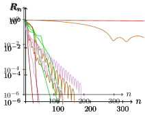
$\lambda=10^{-1}$	$\lambda=10^{-2}$	$\lambda=10^{-4}$

Figure 1: Results for from Section III-A on the influence of $\lambda$.

III-B Influence of the sparsity level

While the construction of a test instance is independent of the parameter $\lambda$, it gets harder for less sparsity. The behavior of the solvers with respect to the sparsity level is illustrated by this example:

Dimensions:

• $n={2000}$ variables,

• $k={200}$ measurements

Matrix $A$:

Bernoulli ensemble, i.e. random $\pm 1$

Solution $x^{*}$:

$s={4,\,80}$ non-zero entries, respectively; magnitude normally distributed with mean zero and variance one.

$\lambda$:

$10^{-1}$

Results:

Most solvers take longer for less sparsity; however, surprisingly, YALL1 is even faster for lower sparsity, see Figure 2.

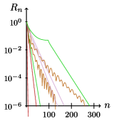
$s=4$	$s=80$

Figure 2: Results for from Section III-B on the influence of the sparsity level $s$.

III-C Influence of the dynamic range of the entries in $x^{*}$

As claimed in the introduction, the dynamic range

$$\Theta(x^{*})=\frac{\max\{|{x^{*}}|\,:\,x^{*}\neq 0\}}{\min\{|{x^{*}}|\,:\,x^{*}\neq 0\}}$$

also influences the performance.

Dimensions:

• $n={3000}$ variables,

• $k={1000}$ measurements

Matrix $A$:

Union of three orthonormal basis: the identity matrix, the DCT matrix and an orthonormalized random matrix

Solution $x^{*}$:

$s={50}$ non-zero entries, with a dynamic range of approximately 9, 701 and 55.000, respectively.

$\lambda$:

$10^{-1}$

Results:

Some solvers dramatically slow down for larger dynamic range, see Figure 3

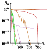
$\Theta(x^{*})\approx 9$	$\Theta(x^{*})\approx 700$	$\Theta(x^{*})\approx 55.000$

Figure 3: Results for from Section III-C on the influence of the dynamic range.

III-D Influence of the coherence of $A$

To illustrate that also a large coherence can cause solvers to slow down, we have chosen the following setup: We considered square matrices $A\in\mathbf{R}^{n\times n}$ which are zero expect on the diagonal and a certain number $K$ of lower off-diagonals, scaled to have $\left\|A\right\|=1$:

$$A_{K} =c\begin{bmatrix}1&0&\cdots&\cdots&\cdots&0\\ \vdots&\ddots&\ddots&&&\vdots\\ 1&&\ddots&\ddots&&\vdots\\ 0&\ddots&&\ddots&\ddots&\vdots\\ \vdots&\ddots&\ddots&&\ddots&0\\ 0&\cdots&0&1&\cdots&1\end{bmatrix}.$$

$$\hskip 86.11084pt\underbrace{\hskip 47.36096pt}_{K\ \text{columns}}$$

We also considered the extreme case $K=n$, also known as the Heaviside matrix. Denoting the columns of $A_{K}$ by $a_{j}$, we calculate the coherence of the matrix $A_{K}$ as

$$\mu=\max_{i\neq j}\frac{\left.\left\langle a_{i}\vphantom{a_{j}}\right|a_{j}\right\rangle}{\left\|a_{i}\right\|\left\|a_{j}\right\|}=\sqrt{\frac{K-1}{K}}.$$

Dimensions:

• $n={300}$ variables,

• $k={300}$ measurements

Matrix $A$:

Increasingly coherent matrices with $K=5,\,40,\,100,\,300$

Solution $x^{*}$:

$s={30}$ non-zero entries, Bernoulli, i.e. randomly selected $+1$ and $-1$.

$\lambda$:

$10^{-1}$

Results:

This problem, while with an square and invertible matrix, is known the be notoriously hard. Especially for large $K$ all solvers deteriorate, see Figure 4.

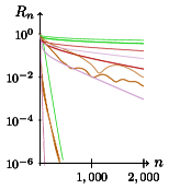
$K=5$, $\mu=0.89$	$K=40$, $\mu=0.987$	$K=100$, $\mu=0.995$	$K=300$, $\mu=0.998$

Figure 4: Results for from Section III-D on the influence of the coherence.

Appendix A Algorithms

Instead of $y\in\mathbf{R}^{m}$ we construct a vector $w\in\mathbf{R}^{n}$ such that

$$w\in\operatorname{rg}A^{T}\cap\operatorname{Sign}(x^{*})$$

which can be reformulated as

$$\begin{split}w_{i}&=1,\quad i\in\mathcal{A}_{+}\\ w_{i}&=-1,\quad i\in\mathcal{A}_{-}\\ |w_{i}|&\leq 1,\quad i\in\mathcal{I}\end{split}$$

and $w\in\operatorname{rg}A^{T}$. Then $y$ can be found by solving $A^{T}y=w$.

A-A Solution by projection onto convex sets

The condition $w\in\operatorname{rg}A^{T}\cap\operatorname{Sign}(x^{*})$ can be seen as a convex feasibility problem [1] since both the sets $\operatorname{rg}A^{T}$ and $\operatorname{Sign}(x^{*})$ are convex. Moreover, the projection onto each set is computationally feasible: The projection onto the range of $A^{T}$ can be calculated explicitly, e.g. with the help of QR factorization. If $A^{T}=QR$ with orthonormal $Q$ and upper triangular $R$, the projection $P_{\operatorname{rg}A^{T}}$ is given by $P_{rgA^{T}}=Q(:,1:k)Q(:,1:k)^{T}$. Projecting onto the convex set $\operatorname{Sign}(x^{*})$ is even simpler: Set the fixed components to $\pm 1$ respectively and clip the others by $x\mapsto\max(\min(x,1)x,-1)$. We done the projection onto $\operatorname{Sign}(x^{*})$ by $P_{\operatorname{Sign}(x^{*})}$.

Now we find $w$ by alternatingly project an initial guess onto both sets, a strategy knows as projection onto convex sets (POCS) [8, 19]. This is given as pseudo code in Algorithm 1.

Algorithm 1 Calculation of $y$ by POCS

0:  Input $A\in\mathbf{R}^{m\times n}$, a partition $\mathcal{A}_{+}$, $\mathcal{A}_{-}$ and $\mathcal{I}$ of $\{1,\dots,n\}$ (coded as $\operatorname{Sign}(x^{*})$), a tolerance $\epsilon>0$ and an initial guess $w_{0}$.

1:  for $i=0,1,\dots$ do

2:     $v^{n}=P_{\operatorname{rg}A^{T}}w^{n}$

3:     $w^{n+1}=P_{\operatorname{Sign}(x^{*})}v^{n}$

4:     if $\max(\left\|v^{n}-w^{n}\right\|,\left\|w^{n+1}-v^{n}\right\|)\leq\epsilon$ then

5:        break

6:     end if

7:  end for

8:  Solve $A^{T}y=w$

9:  return  $y$

A-B Solution by quadratic programming

We sketch another approach by quadratic programming: We call $\mathcal{A}=\mathcal{A}_{+}\cup\mathcal{A}_{-}$ the active set and $\mathcal{I}$ the inactive set and define $s\in\mathbf{R}^{\mathcal{A}}$ by

$$\begin{split}s_{i}&=1,\quad i\in\mathcal{A}_{+}\\ s_{i}&=-1,\quad i\in\mathcal{A}_{-}.\end{split}$$ (3)

Furthermore we denote with $P_{\mathcal{A}}:\mathbf{R}^{n}\to\mathbf{R}^{\mathcal{A}}$ the projection which deletes the “inactive” components and with $P_{\mathcal{I}}:\mathbf{R}^{n}\to\mathbf{R}^{\mathcal{I}}$ the projection which deletes in “active” components and the respective adjoint $P_{\mathcal{A}}^{T}$ and $P_{\mathcal{I}}^{T}$ which fill up the vectors be zeros. With this notation, we aim at finding $w\in\operatorname{rg}A^{T}$ such that

$$P_{\mathcal{A}}w=s,\ \text{ and }\ \left\|P_{\mathcal{I}}w\right\|_{\infty}\leq 1.$$

To fulfill the condition $w\in\operatorname{rg}A^{T}$ we use the orthogonal projection on $\operatorname{rg}A^{T}$, denoted by $P_{\operatorname{rg}A^{T}}$ and require $P_{\operatorname{rg}A^{T}}w=w$. Since $w$ is determined on the active set $\mathcal{A}$ we rewrite is as

$$w=P_{\mathcal{A}}^{T}s+P_{\mathcal{I}}^{T}z$$ (4)

with a $z\in\mathbf{R}^{\mathcal{I}}$. Putting this together we have to find a vector $z\in\mathbf{R}^{\mathcal{I}}$ such that

$$(P_{\operatorname{rg}A^{T}}-\operatorname{Id})P_{\mathcal{I}}^{T}z=(\operatorname{Id}-P_{\operatorname{rg}A^{T}})P_{\mathcal{A}}^{T}s,\quad\left\|z\right\|_{\infty}\leq 1.$$

We the abbreviations

$$\begin{split}\bar{P}&=(P_{\operatorname{rg}A^{T}}-\operatorname{Id})P_{\mathcal{I}}^{T}\\ \bar{v}&=(\operatorname{Id}-P_{\operatorname{rg}A^{T}})P_{\mathcal{A}}^{T}s\end{split}$$ (5)

we reformulate this as the optimization problem

$$\min_{z\in\mathbf{R}^{\mathcal{I}}}\tfrac{1}{2}\left\|\bar{P}z-\bar{v}\right\|^{2}\ \text{s.t.}\ \left\|z\right\|_{\infty}\leq 1.$$ (6)

This quadratic programming or constrained regression problem can be solved by various methods [5] including the simple gradient projection [15] or the conditional gradient method [14, 2]. Note that we require that the optimal value of (6) is indeed zero.

Algorithm 2 gives pseudo-code for calculating $y$.

Algorithm 2 Calculation of $y$ by quadratic programming

0:  Input $A\in\mathbf{R}^{m\times n}$ and a partition $\mathcal{A}_{+}$, $\mathcal{A}_{-}$ and $\mathcal{I}$ of $\{1,\dots,n\}$.

1:  Set $s$ according to (3).

2:  Calculate the projection matrix $P_{\operatorname{rg}A^{T}}$ (e.g. by QR-factorization or singular value decomposition) and define $\bar{P}$ and $\bar{v}$ according to (5).

3:  Calculate $z$ as a solution of (6).

4:  if $\bar{P}z=\bar{v}$ then

5:     calculate $w$ according to (4)

6:  else

7:     return “Error: No solution with this sign-pattern”

8:  end if

9:  Solve $A^{T}y=w$

10:  return  $y$

References

- [1] Heinz H. Bauschke and Jonathan M. Borwein. On projection algorithms for solving convex feasibility problems. SIAM Review, 38(3):367–426, 1996.
- [2] Amir Beck and Marc Teboulle. A conditional gradient method with linear rate of convergence for solving convex linear systems. Mathematical Methods of Operations Research, 59:235–247, 2004.
- [3] Amir Beck and Marc Teboulle. Fast iterative shrinkage-thresholding algorithm for linear inverse problems. SIAM Journal on Imaging Sciences, 2:183–202, 2009.
- [4] Stephen Becker, Jérôme Bobin, and Emmanuel J. Candès. NESTA: A fast and accurate first-order method for sparse recovery. arxiv 0904.3367, 2009.
- [5] Stephen Boyd and Lieven Vandenberghe. Convex optimization. Cambridge University Press, Cambridge, 2004.
- [6] Kristian Bredies and Dirk A. Lorenz. Iterated hard shrinkage for minimization problems with sparsity constraints. SIAM Journal on Scientific Computing, 30(2):657–683, 2008.
- [7] Scott Shaobing Chen, David L. Donoho, and Michael A. Saunders. Atomic decomposition by basis pursuit. SIAM Journal on Scientific Computing, 20(1):33–61, 1998.
- [8] Ward Cheney and Allen A. Goldstein. Proximity maps for convex sets. Proceedings of the American Mathematical Society, 10:448–450, 1959.
- [9] Ingrid Daubechies, Michel Defrise, and Christine De Mol. An iterative thresholding algorithm for linear inverse problems with a sparsity constraint. Communications in Pure and Applied Mathematics, 57(11):1413–1457, 2004.
- [10] Loïc Denis, Dirk Lorenz, Eric Thiébaut, Corinne Fournier, and Dennis Trede. Inline hologram reconstruction with sparsity constraints. Opt. Lett., 34(22):3475–3477, 2009.
- [11] Mário A. T. Figueiredo, Robert D. Nowak, and Stephen J. Wright. Gradient projection for sparse reconstruction: Applications to compressed sensing and other inverse problems. IEEE Journal of Selected Topics in Signal Processing, 4:586–597, 2007.
- [12] Mário A. T. Figueiredo, Robert D. Nowak, and Stephen J. Wright. Sparse reconstruction by separable approximation. IEEE Transactions on Signal Processing, 57:2479–2493, 2009.
- [13] Massimo Fornasier and Holger Rauhut. Recovery algorithms for vector valued data with joint sparsity constraints. SIAM Journal on Numerical Analysis, 46(2):577–613, 2008.
- [14] M. Frank and P. Wolfe. An algorithm for quadratic programming. Naval Research Logistics Quaterly, 3:95–110, 1956.
- [15] A. A. Goldstein. On steepest descent. SIAM Journal on Control and Optimization, 3:147–151, 1965.
- [16] Markus Grasmair, Markus Haltmeier, and Otmar Scherzer. Sparse regularization with penalty term. Inverse Problems, 24(5):055020 (13pp), 2008.
- [17] Markus Grasmair, Otmar Scherzer, and Markus Haltmeier. Necessary and sufficient conditions for linear convergence of -regularization. Communications on Pure and Applied Mathematics, 64:161–182, 2011.
- [18] Roland Griesse and Dirk A. Lorenz. A semismooth Newton method for Tikhonov functionals with sparsity constraints. Inverse Problems, 24(3):035007 (19pp), 2008.
- [19] L. G. Gurin, Boris Teodorovich Poljak, and È. V. Raĭk. Projection methods for finding a common point of convex sets. Akademija Nauk SSSR. Žurnal Vyčislitel′ noĭ Matematiki i Matematičeskoĭ Fiziki, 7:1211–1228, 1967.
- [20] Elaine T. Hale, Wotao Yin, and Yin Zhang. Fixed-point continuation for -minimization: Methodology and convergence. SIAM Journal on Optimization, 19(3):1107–1130, 2008.
- [21] Honglak Lee, Alexis Battle, Rajat Raina, and Andrew Y. Ng. Efficient sparse coding algorithms. In Proceedings of the Neural Information Processing Systems (NIPS), volume 19, 2006.
- [22] Dirk A. Lorenz. Convergence rates and source conditions for Tikhonov regularization with sparsity constraints. Journal of Inverse and Ill-Posed Problems, 16(5):463–478, 2008.
- [23] Dirk A. Lorenz, Stefan Schiffler, and Dennis Trede. Beyond convergence rates: Exact inversion with Tikhonov regularization with sparsity constraints. Submitted for publication, arxiv 1001.3276, 2010.
- [24] Ignace Loris. L1packv2: A mathematica package for minimizing an -penalized functional. Computer Physics Communications, 179:895–902, 2008.
- [25] Ignace Loris. On the performance of algorithms for the minimization of -penalized functionals. Inverse Problems, 25:035008 (16pp), 2009.
- [26] Moshe Mishali and Yonina C. Eldar. Reduce and boost: recovering arbitrary sets of jointly sparse vectors. IEEE Transactions on Signal Processing, 56(10, part 1):4692–4702, 2008.
- [27] Ronny Ramlau. Regularization properties of Tikhonov regularization with sparsity constraints. Electronic Transactions on Numerical Analysis, 30:54–74, 2008.
- [28] Benjamin Recht, Maryam Fazel, and Pablo A. Parrilo. Guaranteed minimum rank solutions to linear matrix equations via nuclear norm minimization. SIAM Review, 52(3):471–501, 2010.
- [29] Robert Tibshirani. Regression shrinkage and selection via the lasso. Journal of the Royal Statistical Society. Series B, 58(1):267–288, 1996.
- [30] Joel A. Tropp. Just relax: Convex programming methods for identifying sparse signals in noise. IEEE Transactions on Information Theory, 52(3):1030–1051, March 2006.
- [31] Ewout van den Berg and Michael P. Friedlander. Probing the Pareto frontier for basis pursuit solutions. SIAM Journal on Scientific Computing, 31(2):890–912, 2008.
- [32] Ewout van den Berg and Michael P. Friedlander. Joint-sparse recovery from multiple measurements. Department of Computer Science, University of British Columbia, Technical Report TR-2009-07, 2009.
- [33] Junfeng Yang and Yin Zhang. Alternating direction algorithms for problems in compressive sensing. Technical report, Rice University, 2009. TR09-37, CAAM.
- [34] Wotao Yin, Stanley J. Osher, Donald Goldfarb, and Jerome Darbon. Bregman iterative algorithms for -minimization with applications to compressed sensing. SIAM Journal on Imaging Sciences, 1(1):143–168, 2008.