Estimation of Saturation of Permanent-Magnet Synchronous Motors Through an Energy-Based Model

Abstract

We propose a parametric model of the saturated Permanent-Magnet Synchronous Motor (PMSM) together with an estimation method of the magnetic parameters. The model is based on an energy function which simply encompasses the saturation effects. Injection of fast-varying pulsating voltages and measurements of the resulting current ripples then permit to identify the magnetic parameters by linear least squares. Experimental results on a surface-mounted PMSM and an interoir magnet PMSM illustrate the relevance of the approach.

Index Terms: Permanent magnet synchronous motor, magnetic circuit modeling, magnetic saturation, energy-based modeling, cross-magnetization

I Introduction

Sensorless control of Permanent-Magnet Synchronous Motors (PMSM) at low velocity remains a challenging task. Most of the existing control algorithms rely on the motor saliency, both geometric and saturation-induced, for extracting the rotor position from the current measurements through high-frequency signal injection [1, 2]. However some magnetic saturation effects such as cross-coupling and permanent magnet demagnetization can introduce large errors on the rotor position estimation [3, 4]. These errors decrease the performance of the controller. In some cases they may cancel the rotor total saliency and lead to instability. It is thus important to correctly model the magnetic saturation effects, which is usually done through d-q magnetizing curves (flux versus current). These curves are usually found either by finite element analysis FEA or experimentally by integration of the voltage equation [5, 6]. This provides a good way to characterize the saturation effects and can be used to improve the sensorless control of the PMSM [7, 8]. However the FEA or the integration of the voltage equation methods are not so easy to implement and do not provide an explicit model of the saturated PMSM.

In this paper a simple parametric model of the saturated PMSM is introduced (section II); it is based on an energy function [9, 10] which simply encompasses the saturation and cross-magnetization effects. In section III a simple estimation method of the magnetic parameters is proposed and rigorously justified: fast-varying pulsating voltages are impressed to the motor with rotor locked; they create current ripples from which the magnetic parameters are estimated by linear least squares. In section IV experimental results on two kinds of motors (with surface-mounted and interior magnets) illustrate the relevance of the approach.

II An energy-based model for the saturated PMSM

II-A Energy-based model

The electrical subsystem of a two-axis PMSM expressed in the synchronous $d-q$ frame reads

$$\frac{d\phi_{d}}{dt} =u_{d}-Ri_{d}+\frac{d\theta}{dt}\phi_{q}$$ (1)

$$\frac{d\phi_{q}}{dt} =u_{q}-Ri_{q}-\frac{d\theta}{dt}(\phi_{d}+\phi_{m}),$$ (2)

where $\phi_{d},\phi_{m}$ are the direct-axis flux linkages due to the current excitation and to the permanent magnet, and $\phi_{q}$ is the quadrature-axis flux linkage; $u_{d},u_{q}$ are the impressed voltages and $i_{d},i_{q}$ are the currents; $\theta$ is the rotor (electrical) position and $R$ is the stator resistance. The currents can be expressed in function of the flux linkages thanks to a suitable energy function ${\mathcal{H}}(\phi_{d},\phi_{q})$ by

$$i_{d} =\partial_{1}{\mathcal{H}}(\phi_{d},\phi_{q})$$ (3)

$$i_{q} =\partial_{2}{\mathcal{H}}(\phi_{d},\phi_{q}),$$ (4)

where $\partial_{k}{\mathcal{H}}$ denotes the partial derivative w.r.t. the $k^{th}$ variable, see [9, 10]; without loss of generality ${\mathcal{H}}(0,0)=0$.

For an unsaturated PMSM this energy function reads

$${\mathcal{H}}_{l}(\phi_{d},\phi_{q}) =\frac{1}{2L_{d}}\phi^{2}_{d}+\frac{1}{2L_{q}}\phi^{2}_{q}$$

where $L_{d}$ and $L_{q}$ are the motor self-inductances, and we recover the usual linear relations

$$i_{d} =\partial_{1}{\mathcal{H}}(\phi_{d},\phi_{q})=\frac{\phi_{d}}{L_{d}}$$

$$i_{q} =\partial_{2}{\mathcal{H}}(\phi_{d},\phi_{q})=\frac{\phi_{q}}{L_{q}}.$$

Notice the expression for ${\mathcal{H}}$ should respect the symmetry of the PMSM w.r.t the direct axis, i.e.

$${\mathcal{H}}(\phi_{d},-\phi_{q})={\mathcal{H}}(\phi_{d},\phi_{q}),$$ (5)

which is obviously the case for ${\mathcal{H}}_{l}$. Indeed, (1)-(2) is left unchanged by the transformation

$$(\phi_{d}^{\prime},u_{d}^{\prime},i_{d}^{\prime},\phi_{q}^{\prime},u_{q}^{\prime},i_{q}^{\prime},\theta^{\prime}):=(\phi_{d},u_{d},i_{d},-\phi_{q},-u_{q},-i_{q},-\theta);$$

this implies

$$\partial_{1}{\mathcal{H}}(\phi_{d}^{\prime},\phi_{q}^{\prime}) =\partial_{1}{\mathcal{H}}(\phi_{d},\phi_{q})$$

$$\partial_{2}{\mathcal{H}}(\phi_{d}^{\prime},\phi_{q}^{\prime}) =-\partial_{2}{\mathcal{H}}(\phi_{d},\phi_{q}),$$

i.e.

$$\partial_{1}{\mathcal{H}}(\phi_{d},-\phi_{q}) =\partial_{1}{\mathcal{H}}(\phi_{d},\phi_{q})$$

$$\partial_{2}{\mathcal{H}}(\phi_{d},-\phi_{q}) =-\partial_{2}{\mathcal{H}}(\phi_{d},\phi_{q}).$$

Therefore

$$\frac{d{\mathcal{H}}}{d\phi_{d}}(\phi_{d},-\phi_{q}) =\partial_{1}{\mathcal{H}}(\phi_{d},-\phi_{q})$$

$$=\partial_{1}{\mathcal{H}}(\phi_{d},\phi_{q})$$

$$=\frac{d{\mathcal{H}}}{d\phi_{d}}(\phi_{d},\phi_{q})$$

$$\frac{d{\mathcal{H}}}{d\phi_{q}}(\phi_{d},-\phi_{q}) =-\partial_{2}{\mathcal{H}}(\phi_{d},-\phi_{q})$$

$$=\partial_{2}{\mathcal{H}}(\phi_{d},\phi_{q})$$

$$=\frac{d{\mathcal{H}}}{d\phi_{q}}(\phi_{d},\phi_{q}).$$

Integrating these relations yields

$${\mathcal{H}}(\phi_{d},-\phi_{q}) ={\mathcal{H}}(\phi_{d},\phi_{q})+c_{d}(\phi_{q})$$

$${\mathcal{H}}(\phi_{d},-\phi_{q}) ={\mathcal{H}}(\phi_{d},\phi_{q})+c_{q}(\phi_{d}),$$

where $c_{d},c_{q}$ are functions of only one variable. But this makes sense only if $c_{d}(\phi_{q})=c_{q}(\phi_{d})=c$ with $c$ constant. Since $H(0,0)=0$, $c=0$, which yields (5).

II-B Parametric description of magnetic saturation

Magnetic saturation can be accounted for by considering a more complicated magnetic energy function ${\mathcal{H}}$, having ${\mathcal{H}}_{l}$ for quadratic part but including also higher-order terms. From experiments saturation effects are well captured by considering only third- and fourth-order terms, hence

$${\mathcal{H}}(\phi_{d},\phi_{q})={\mathcal{H}}_{l}(\phi_{d},\phi_{q})\\ +\sum_{i=0}^{3}\alpha_{3-i,i}\phi_{d}^{3-i}\phi_{q}^{i}+\sum_{i=0}^{4}\alpha_{4-i,i}\phi_{d}^{4-i}\phi_{q}^{i}.$$

This is a perturbative model where the higher-order terms appear as corrections of the dominant term ${\mathcal{H}}_{l}$. The $9$ coefficients $\alpha_{ij}$ together with $L_{d}$, $L_{q}$ are motor dependent. But (5) implies $\alpha_{2,1}=\alpha_{0,3}=\alpha_{3,1}=\alpha_{1,3}=0$, so that the energy function eventually reads

$${\mathcal{H}}(\phi_{d},\phi_{q})={\mathcal{H}}_{l}(\phi_{d},\phi_{q})+\alpha_{3,0}\phi_{d}^{3}+\alpha_{1,2}\phi_{d}\phi_{q}^{2}\\ +\alpha_{4,0}\phi_{d}^{4}+\alpha_{2,2}\phi_{d}^{2}\phi_{q}^{2}+\alpha_{0,4}\phi_{q}^{4}.$$ (6)

From (3)-(4) and (6) the currents are then explicitly given by

$$i_{d} =\partial_{1}{\mathcal{H}}(\phi_{d},\phi_{q})$$

$$=\frac{\phi_{d}}{L_{d}}+3\alpha_{3,0}\phi_{d}^{2}+\alpha_{1,2}\phi_{q}^{2}+4\alpha_{4,0}\phi_{d}^{3}+2\alpha_{2,2}\phi_{d}\phi_{q}^{2}$$ (7)

$$i_{q} =\partial_{2}{\mathcal{H}}(\phi_{d},\phi_{q})$$

$$=\frac{\phi_{q}}{L_{q}}+2\alpha_{1,2}\phi_{d}\phi_{q}+2\alpha_{2,2}\phi_{d}^{2}\phi_{q}+4\alpha_{0,4}\phi_{q}^{3},$$ (8)

which are the flux-current magnetization curves. Fig. 1 shows examples of these curves in the more familiar presentation of fluxes w.r.t currents obtained by numerically inverting (3)-(4); the motor is the IPM of section IV.

The model of the saturated PMSM is thus given by (1)-(2) and (7)-(8). It is in state form with $\phi_{d},\phi_{q}$ as state variables. The magnetic saturation effects are represented by the $5$ additional parameters $\alpha_{3,0},\alpha_{1,2},\alpha_{4,0},\alpha_{2,2},\alpha_{0,4}$.

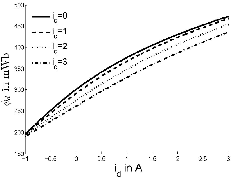
(a) $\phi_{d}(i_{d},i_{q}=Constant)$

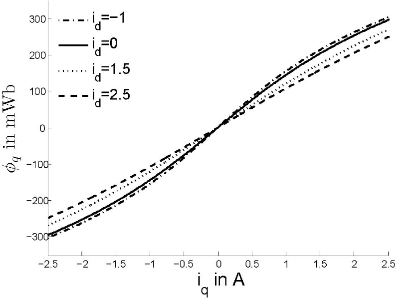
(b) $\phi_{q}(i_{d}=Constant,i_{q})$

Figure 1: Flux-current magnetization curves (IPM)

II-C Model with $i_{d},i_{q}$ as state variables

The model of the saturated PMSM is often expressed with $i_{d},i_{q}$ as state variables, e.g. [5]. Starting with flux-current magnetization curves in the form

$$\phi_{d} =\Phi_{d}(i_{d},i_{q})$$ (9)

$$\phi_{q} =\Phi_{q}(i_{d},i_{q})$$ (10)

and differentiating w.r.t time, (1)-(2) then becomes

$$L_{dd}(i_{d},i_{q})\frac{di_{d}}{dt}+L_{dq}(i_{d},i_{q})\frac{di_{q}}{dt} =u_{d}-Ri_{d}+\frac{d\theta}{dt}\phi_{q}$$

$$L_{qd}(i_{d},i_{q})\frac{di_{d}}{dt}+L_{qq}(i_{d},i_{q})\frac{di_{q}}{dt} =u_{q}-Ri_{q}-\frac{d\theta}{dt}(\phi_{d}+\phi_{m}),$$

where

$$\begin{pmatrix}L_{dd}(i_{d},i_{q})&L_{dq}(i_{d},i_{q})\\ L_{qd}(i_{d},i_{q})&L_{qq}(i_{d},i_{q})\end{pmatrix}= \begin{pmatrix}\partial_{1}\Phi_{d}(i_{d},i_{q})&\partial_{2}\Phi_{d}(i_{d},i_{q})\\ \partial_{1}\Phi_{q}(i_{d},i_{q})&\partial_{2}\Phi_{q}(i_{d},i_{q})\end{pmatrix}.$$

Though not always acknowledged $L_{dq}$ and $L_{qd}$ should be equal. Indeed, plugging (3)-(4) into (9)-(10) gives

$$\phi_{d} =\Phi_{d}\bigl{(}\partial_{1}{\mathcal{H}}(\phi_{d},\phi_{q}),\partial_{2}{\mathcal{H}}(\phi_{d},\phi_{q})\bigr{)}$$

$$\phi_{q} =\Phi_{q}\bigl{(}\partial_{1}{\mathcal{H}}(\phi_{d},\phi_{q}),\partial_{2}{\mathcal{H}}(\phi_{d},\phi_{q})\bigr{)}.$$

Taking the total derivative of both sides of these equations w.r.t. $\phi_{d}$ and $\phi_{q}$ then yields

$$\begin{pmatrix}1&0\\ 0&1\end{pmatrix}= \begin{pmatrix}L_{dd}\partial_{11}{\mathcal{H}}+L_{dq}\partial_{12}{\mathcal{H}}&L_{dd}\partial_{21}{\mathcal{H}}+L_{dq}\partial_{22}{\mathcal{H}}\\ L_{qd}\partial_{11}{\mathcal{H}}+L_{qq}\partial_{12}{\mathcal{H}}&L_{qd}\partial_{21}{\mathcal{H}}+L_{qq}\partial_{22}{\mathcal{H}}\end{pmatrix}$$

$$= \begin{pmatrix}L_{dd}&L_{dq}\\ L_{qd}&L_{qq}\end{pmatrix}\begin{pmatrix}\partial_{11}{\mathcal{H}}&\partial_{21}{\mathcal{H}}\\ \partial_{12}{\mathcal{H}}&\partial_{22}{\mathcal{H}}\end{pmatrix}.$$

Since $\partial_{12}{\mathcal{H}}=\partial_{21}{\mathcal{H}}$ the second matrix in the last line is symmetric, hence the first; in other words $L_{dq}=L_{qd}$.

To do that with the model of section II-B the nonlinear equations (7)-(8) must be inverted. Rather than doing that exactly, we take advantage of the fact the coefficients $\alpha_{i,j}$ are experimentally small. At first order w.r.t. the $\alpha_{i,j}$ we obviously have $\phi_{d}=L_{d}i_{d}+{\mathcal{O}}(\left\lvert\alpha_{i,j}\right\rvert)$ and $\phi_{q}=L_{q}i_{q}+{\mathcal{O}}(\left\lvert\alpha_{i,j}\right\rvert)$. Plugging these expressions into (7)-(8) we easily find

$$\phi_{d} =L_{d}\bigl{(}i_{d}-3\alpha_{3,0}L_{d}^{2}i_{d}^{2}-\alpha_{1,2}L_{q}^{2}i_{q}^{2}-4\alpha_{4,0}L_{d}^{3}i_{d}^{3}$$

$$\quad-2\alpha_{2,2}L_{d}L_{q}^{2}i_{d}i_{q}^{2}\bigr{)}+{\mathcal{O}}(\left\lvert\alpha_{i,j}\right\rvert^{2})$$ (11)

$$\phi_{q} =L_{q}\bigl{(}i_{q}-2\alpha_{1,2}L_{d}L_{q}i_{d}i_{q}-2\alpha_{2,2}L_{d}^{2}L_{q}i_{d}^{2}i_{q}$$

$$\quad-4\alpha_{0,4}L_{q}^{3}i_{q}^{3}\bigr{)}+{\mathcal{O}}(\left\lvert\alpha_{i,j}\right\rvert^{2}).$$ (12)

Finally,

$$L_{dd}(i_{d},i_{q}) =L_{d}\bigl{(}1-6\alpha_{3,0}L_{d}i_{d}-12\alpha_{4,0}L_{d}^{2}i_{d}^{2}-2\alpha_{2,2}L_{q}^{2}i_{q}^{2}\bigr{)}$$

$$L_{dq}(i_{d},i_{q}) =L_{qd}(i_{d},i_{q})=-2L_{d}L_{q}^{2}i_{q}(\alpha_{1,2}+2\alpha_{2,2}L_{d}i_{d})$$

$$L_{qq}(i_{d},i_{q}) =L_{q}\bigl{(}1-2\alpha_{1,2}L_{d}i_{d}-2\alpha_{2,2}L_{d}^{2}i_{d}^{2}-12\alpha_{0,4}L_{q}^{2}i_{q}^{2}\bigr{)}.$$

III A procedure for estimating the magnetic parameters

III-A Principle

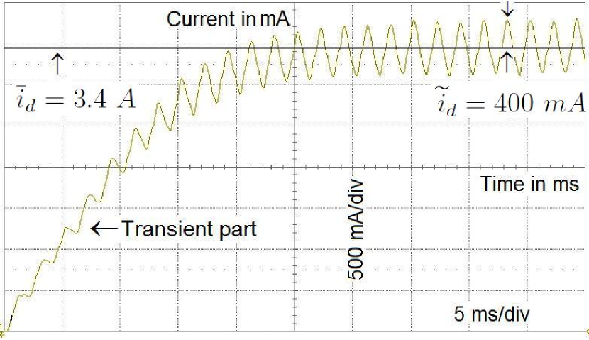
Figure 2: Experimental illustration of equation (15): time response of $i_{d}$

To estimate the $7$ magnetic parameters in the model, we propose a procedure which is rather easy to implement and reliable. With the rotor locked in the position $\theta=0$, we inject fast-varying pulsating voltages

$$u_{d}(t) =\bar{u}_{d}+\widetilde{u}_{d}f({\Omega}t)$$ (13)

$$u_{q}(t) =\bar{u}_{q}+\widetilde{u}_{q}f({\Omega}t),$$ (14)

where $\bar{u}_{d},\bar{u}_{q},\widetilde{u}_{d},\widetilde{u}_{q},{\Omega}$ are constant and $f$ is a periodic function with zero mean. The pulsation ${\Omega}$ is chosen large enough w.r.t. the motor electric time constant. It can then be shown, see section III-C, that after an initial transient

$$i_{d}(t) =\bar{i}_{d}+\widetilde{i}_{d}F({\Omega}t)+{\mathcal{O}}(\tfrac{1}{{\Omega}^{2}})$$ (15)

$$i_{q}(t) =\bar{i}_{q}+\widetilde{i}_{q}F({\Omega}t)+{\mathcal{O}}(\tfrac{1}{{\Omega}^{2}}),$$ (16)

where $\bar{i}_{d}=\frac{\bar{u}_{d}}{R},\bar{i}_{q}=\frac{\bar{u}_{q}}{R},\widetilde{i}_{d},\widetilde{i}_{q}$ are constant and $F$ is the primitive of $f$ with zero mean ($F$ has clearly the same period as $f$); fig. 2 shows for instance the current $i_{d}$ obtained for the SPM of section IV when starting from $i_{d}(0)=0$ and applying a square signal $u_{d}$ with $\Omega=500Hz$, $\bar{u}_{d}=23V$ and $\widetilde{u}_{d}=30V$. On the other hand using the saturation model the amplitudes $\widetilde{i}_{d},\widetilde{i}_{q}$ of the current ripples turn out to be

$$\widetilde{i}_{d} =\frac{1}{{\Omega}}\Bigl{(}\frac{\widetilde{u}_{d}}{L_{d}}+2\alpha_{2,2}L_{q}\bar{i}_{q}(2L_{d}\bar{i}_{d}\widetilde{u}_{q}+L_{q}\bar{i}_{q}\widetilde{u}_{d})$$

$$\quad+12\alpha_{4,0}L_{d}^{2}\bar{i}_{d}^{2}\widetilde{u}_{d}+6\alpha_{3,0}L_{d}\bar{i}_{d}\widetilde{u}_{d}+2\alpha_{1,2}L_{q}\bar{i}_{q}\widetilde{u}_{q}\Bigr{)}$$ (17)

$$\widetilde{i}_{q} =\frac{1}{{\Omega}}\Bigl{(}\frac{\widetilde{u}_{q}}{L_{q}}+2\alpha_{2,2}L_{d}\bar{i}_{d}(2L_{q}\bar{i}_{q}\widetilde{u}_{d}+L_{d}\bar{i}_{d}\widetilde{u}_{q})$$

$$\quad+12\alpha_{0,4}L_{q}^{2}\bar{i}_{q}^{2}\widetilde{u}_{q}+2\alpha_{1,2}(L_{d}\bar{i}_{d}\widetilde{u}_{q}+L_{q}\bar{i}_{q}\widetilde{u}_{d})\Bigr{)}.$$ (18)

As $\widetilde{i}_{d},\widetilde{i}_{q}$ can easily be measured experimentally, these expressions provide a means to identify the magnetic parameters from experimental data obtained with various values of $\bar{u}_{d},\bar{u}_{q},\widetilde{u}_{d},\widetilde{u}_{q}$.

III-B Estimation of the parameters

Since combinations of the magnetic parameters always enter (17)-(18) linearly, they can be estimated by simple linear least squares; moreover by suitably choosing $\bar{u}_{d},\bar{u}_{q},\widetilde{u}_{d},\widetilde{u}_{q}$, the whole least squares problem for the $7$ parameters can be split into several problems involving fewer parameters:

• with $\bar{u}_{d}=\bar{u}_{q}=0$, hence $\bar{i}_{d}=\bar{i}_{q}=0$, and $\widetilde{u}_{d}=0$ (resp. $\widetilde{u}_{q}=0$) equation (17) (resp. equation (18)) reads

  $$L_{d}=\frac{1}{{\Omega}}\frac{\widetilde{u}_{d}}{\widetilde{i}_{d}}\qquad\Bigl{(}\text{resp.~{}~{}}L_{q}=\frac{1}{{\Omega}}\frac{\widetilde{u}_{q}}{\widetilde{i}_{q}}\Bigr{)}$$ (19)

• with $\bar{u}_{q}=0$, hence $\bar{i}_{q}=0$, and $\widetilde{u}_{q}=0$, (17) reads

  $$\widetilde{i}_{d}=\frac{\widetilde{u}_{d}}{{\Omega}}\left(\frac{1}{L_{d}}+6\alpha_{3,0}L_{d}\bar{i}_{d}+12\alpha_{4,0}L_{d}^{2}\bar{i}_{d}^{2}\right).$$ (20)

  Notice (18) reads $\widetilde{i}_{q}=0$ hence provides no information

• with $\bar{u}_{d}=0$, hence $\bar{i}_{d}:=0$, and $\widetilde{u}_{q}=0$, (17)-(18) read

  $$\widetilde{i}_{d} =\frac{\widetilde{u}_{d}}{{\Omega}}\Bigl{(}\frac{1}{L_{d}}+2\alpha_{2,2}L_{q}^{2}\bar{i}_{q}^{2}\Bigr{)}$$ (21)

  $$\widetilde{i}_{q} =\frac{2\widetilde{u}_{d}}{{\Omega}}\alpha_{1,2}L_{q}\bar{i}_{q}$$ (22)

• with $\bar{u}_{d}=0$, hence $\bar{i}_{d}:=0$, and $\widetilde{u}_{d}=0$, (17)-(18) read

  $$\widetilde{i}_{d} =\frac{2\widetilde{u}_{q}}{{\Omega}}\alpha_{1,2}L_{q}\bar{i}_{q}$$ (23)

  $$\widetilde{i}_{q} =\frac{\widetilde{u}_{q}}{{\Omega}}\Bigl{(}\frac{1}{L_{q}}+12\alpha_{0,4}L_{q}^{2}\bar{i}_{q}^{2}\Bigr{)}.$$ (24)

$L_{d}$ (resp. $L_{q}$) is then immediately determined from (19); $\alpha_{3,0}$ and $\alpha_{4,0}$ are jointly estimated by least squares from (20); $\alpha_{2,2}$, $\alpha_{1,2}$ and $\alpha_{0,4}$ are separately estimated by least squares from respectively (21), (22)-(23) and (24).

III-C Justification of section III-A

The assertions of section III-A can be rigorously justified by a straightforward application of second-order averaging of differential equations [11, p. 40]. Indeed the electrical subsystem (1)-(2) with locked rotor (i.e. $\frac{d\theta}{dt}=0$) and input voltages (13)-(13) reads when setting $\tau={\Omega}t$

$$\frac{d\phi_{d}}{d\tau} =\frac{1}{{\Omega}}\bigl{(}\bar{u}_{d}+\widetilde{u}_{d}f(\tau)-Ri_{d}(\phi_{d},\phi_{q})\bigr{)}$$ (25)

$$\frac{d\phi_{q}}{d\tau} =\frac{1}{{\Omega}}\bigl{(}\bar{u}_{q}+\widetilde{u}_{q}f(\tau)-Ri_{q}(\phi_{d},\phi_{q})\bigr{)}.$$ (26)

This system is in the so-called standard form for averaging, with a right hand-side periodic in $\tau$ and $\frac{1}{{\Omega}}$ as a small parameter. Therefore its solution is given by

$$\phi_{d}(\tau) =\phi_{d}^{0}(\tau)+\frac{\widetilde{u}_{d}}{{\Omega}}F(\tau)+{\mathcal{O}}(\tfrac{1}{{\Omega}^{2}})$$ (27)

$$\phi_{q}(\tau) =\phi_{q}^{0}(\tau)+\frac{\widetilde{u}_{q}}{{\Omega}}F(\tau)+{\mathcal{O}}(\tfrac{1}{{\Omega}^{2}}),$$ (28)

where $(\phi_{d}^{0},\phi_{q}^{0})$ is the solution of the system

$$\frac{d\phi_{d}^{0}}{dt} =\bar{u}_{d}-Ri_{d}(\phi_{d}^{0},\phi_{q}^{0})$$

$$\frac{d\phi_{q}^{0}}{dt} =\bar{u}_{q}-Ri_{q}(\phi_{d}^{0},\phi_{q}^{0})$$

obtained by averaging the right-hand side of (25)-(26). After an initial transient $\bigl{(}\phi_{d}^{0}(\tau),\phi_{q}^{0}(\tau)\bigr{)}$ asymptotically reaches the constant value $(\bar{\phi}_{d},\bar{\phi}_{q})$ determined by $\bar{u}_{d}=Ri_{d}(\bar{\phi}_{d},\bar{\phi}_{q})$ and $\bar{u}_{q}=Ri_{q}(\bar{\phi}_{d},\bar{\phi}_{q})$.

Plugging (27)-(28) with $t=\frac{\tau}{{\Omega}}$ into (7)-(8), and expanding along powers of $\frac{1}{{\Omega}}$ then yields

$$i_{d}(t) =\bar{i}_{d}+\frac{F({\Omega}t)}{{\Omega}}\biggr{(}\frac{\widetilde{u}_{d}}{L_{d}}+6\alpha_{3,0}\bar{\phi}_{d}\widetilde{u}_{d}+2\alpha_{1,2}\bar{\phi}_{q}\widetilde{u}_{q}$$

$$\quad+12\alpha_{4,0}\bar{\phi}_{d}^{2}\widetilde{u}_{d}+2\alpha_{2,2}(2\bar{\phi}_{d}\bar{\phi}_{q}\widetilde{u}_{q}+\bar{\phi}_{q}^{2}\widetilde{u}_{d})\biggl{)}+{\mathcal{O}}(\tfrac{1}{{\Omega}^{2}})$$

$$i_{q}(t) =\bar{i}_{q}+\frac{F({\Omega}t)}{{\Omega}}\biggl{(}\frac{\widetilde{u}_{q}}{L_{q}}+2\alpha_{1,2}(\bar{\phi}_{d}\widetilde{u}_{q}+\bar{\phi}_{q}\widetilde{u}_{d})$$

$$\quad+2\alpha_{2,2}(2\bar{\phi}_{d}\bar{\phi}_{q}\widetilde{u}_{d}+\bar{\phi}_{d}^{2}\widetilde{u}_{q})+12\alpha_{0,4}\bar{\phi}_{q}^{2}\widetilde{u}_{q}\biggr{)}+{\mathcal{O}}(\tfrac{1}{{\Omega}^{2}}),$$

where $\bar{i}_{d}=i_{d}(\bar{\phi}_{d},\bar{\phi}_{q})$ and $\bar{i}_{q}=i_{q}(\bar{\phi}_{d},\bar{\phi}_{q})$ There remains to express $\bar{\phi}_{d},\bar{\phi}_{q}$ in function of $\bar{i}_{d},\bar{i}_{q}$. Rather than exactly inverting the nonlinear equations (7)-(8), we take advantage of the fact the coefficients $\alpha_{i,j}$ are experimentally small. At first order w.r.t. the $\alpha_{i,j}$ we have $\phi_{d}=L_{d}i_{d}+{\mathcal{O}}(\left\lvert\alpha_{i,j}\right\rvert)$ and $\phi_{q}=L_{q}i_{q}+{\mathcal{O}}(\left\lvert\alpha_{i,j}\right\rvert)$. Using this in the previous equations and neglecting ${\mathcal{O}}(\tfrac{1}{{\Omega}^{2}})$ and ${\mathcal{O}}(\left\lvert\alpha_{i,j}\right\rvert^{2})$ terms we eventually find (15)-(18). Using directly (11)-(12) yields of course the same result.

IV Experimental Results

IV-A Experimental setup

The methodology of section III is tested on an interior magnet PMSM (IPM) and a surface-mounted PMSM (SPM) with rated parameters listed below. The setup consists of an industrial inverter with a $400V$ DC bus and a $4kHz$ PWM switching frequency, 3 dSpace boards (DS1005 PPC Board, DS2003 A/D Board, DS4002 Timing and Digital I/O Board) and a host PC. The measurements were sampled also at $4kHz$.

	IPM	SPM
Pole pairs	6	2
Rated power	$200~{}W$	$1200~{}W$
Rated current	$1.2~{}A$	$3.4~{}A$
Rated speed	$1800~{}rpm$	$400~{}rpm$
Rated torque	$1.06~{}N.m$	$29~{}N.m$
Resistance	$12.15~{}{\Omega}$	$6.69~{}{\Omega}$

IV-B Experimental results

With the rotor locked in the position $\theta=0$, a square wave voltage with frequency ${\Omega}=500Hz$ and constant amplitude $\widetilde{u}_{d}$ or $\widetilde{u}_{q}$ ($30V$ for the IPM, $40V$ for the SPM) is applied to the motor. But for the determination of $L_{d},L_{q}$ where $\bar{u}_{d}=\bar{u}_{q}=0$, several runs are performed with various $\bar{u}_{d}$ (resp. $\bar{u}_{q}$) such that $\bar{i}_{d}$ (resp. $\bar{i}_{q}$) ranges from $-2A$ to $+2A$ with a $0.3A$ increment (IPM), or from $-8A$ to $8A$ with a $0.5A$ increment (SPM). The estimated parameters are listed below; the uncertainty in the estimation stems from a $\pm 10mA$ uncertainty in the current measurements.

	IPM	SPM
$L_{d}~{}(mH$)	$91.9\pm 5$	$155.4\pm 10$
$L_{q}~{}(mH)$	$45.8\pm 1$	$58.6\pm 2$
$\alpha_{3,0}~{}(A.Wb^{-2})$	$7.70\pm 0.11$	$5.01\pm 0.11$
$\alpha_{1,2}~{}(A.Wb^{-2})$	$5.35\pm 0.61$	$4.83\pm 0.27$
$\alpha_{4,0}~{}(A.Wb^{-3})$	$19.42\pm 1.34$	$1.83\pm 0.28$
$\alpha_{2,2}~{}(A.Wb^{-3})$	$22.18\pm 2.80$	$8.76\pm 1.03$
$\alpha_{0,4}~{}(A.Wb^{-3})$	$6.62\pm 0.42$	$1.18\pm 0.17$

The good agreement between the fitted curves and the measurements is demonstrated for instance for (20) on Fig. 3 and for (22) on Fig. 4. Notice (20) illustrates saturation on a single axis, while (22) illustrates cross-saturation.

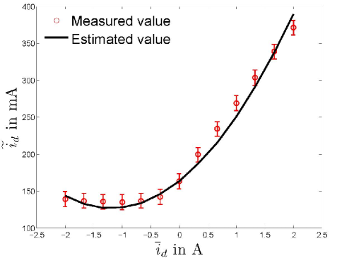
(a) IPM

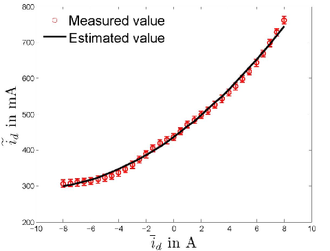
(b) SPM

Figure 3: Measured values (circles) and fitted curve (solid line) for (20).

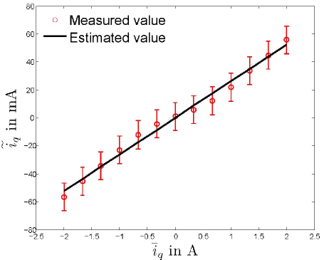
(a) IPM

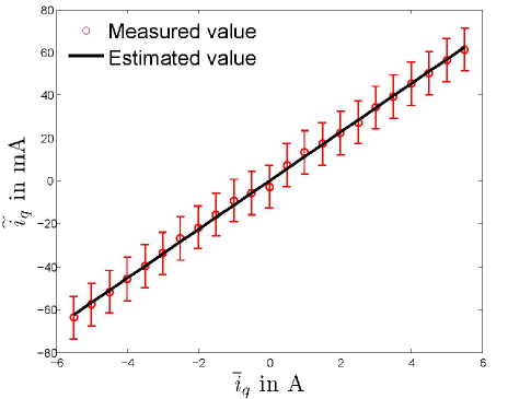
(b) SPM

Figure 4: Measured values (circles) and fitted curve (solid line) for (22).

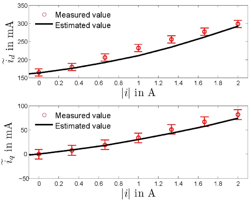
(a) Interior-magnet PMSM

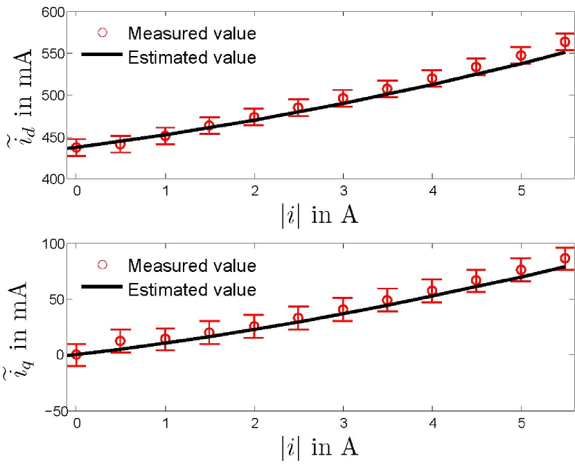
(b) Surface mounted PMSM

Figure 5: Measured values (circles) compared to model-predicted values (solid line) for a $60^{\circ}$ current angle.

IV-C Validation

The estimation procedure relies on (20)–(24), with either $\bar{i}_{d}\neq$ or , i.e. current vectors with angles $0^{\circ},90^{\circ},180^{\circ},270^{\circ}$. To check the validity of the model tests were conducted with current vectors with various angles and magnitudes on the whole operating ($|i|=\sqrt{i_{d}^{2}+i_{q}^{2}}$ ranging from $0A$ to $2A$ with a $0.3A$ increment for the IPM, and from $0A$ to $5.5A$ with a $0.5A$ increment for the SPM). Fig. 5 shows for instance the results for a $60^{\circ}$ current angle; there is a good agreement between the measured values and those predicted by the model.

As a kind of cross-validation we also examined the currents time responses to large voltage steps. Fig. 6 shows the good agreement between the measurements and the time response obtained by simulating the model with the estimated parameters; it also shows the differences with the simulated response when the saturation effects are omitted. Fig. 7 shows the good agreement also between the “measured” flux values (i.e. obtained by integrating the measured currents and voltages) and the flux values obtained by simulation.

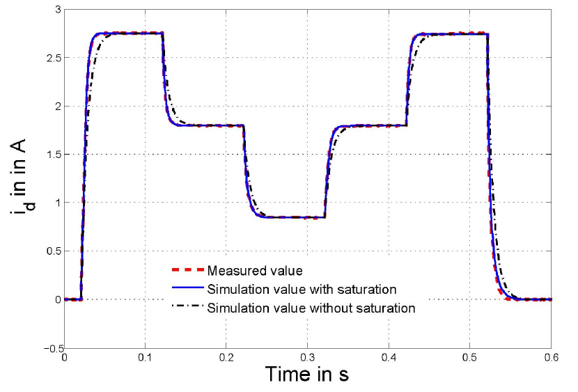
Figure 6: Time response of $i_{d}$ to large step voltages in $u_{d}$ (IPM).

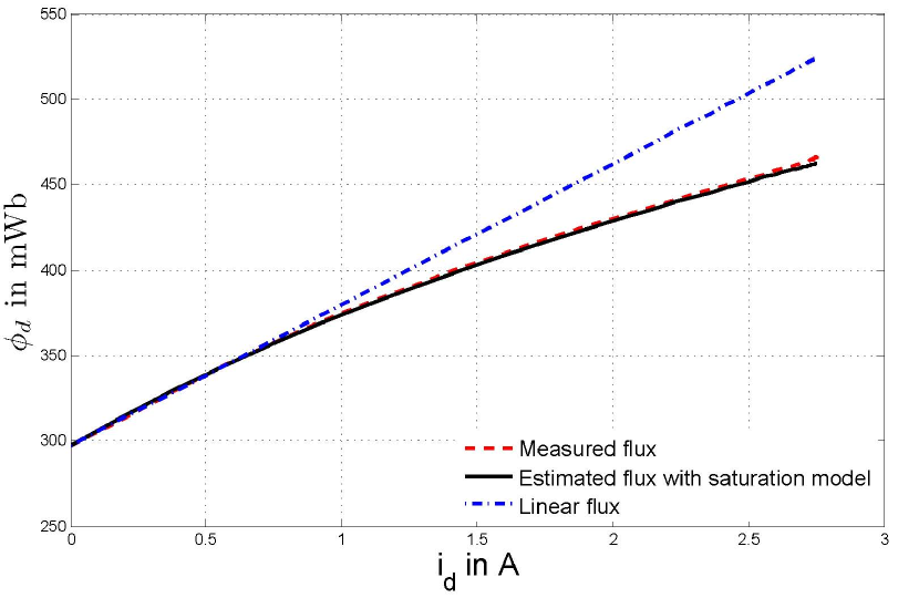
Figure 7: Saturation curve $\phi_{d}-i_{d}$ (IPM).

V Conclusion

A simple parametric magnetic saturation model for the PMSM with a simple identification procedure based on high-frequency voltage injection have been introduced. Experimental tests on two kinds of PMSM (IPM and SPM) demonstrate the relevance of the approach. This model can be fruitfully used to design a sensorless control scheme at low velocity.

References

- [1] J. H. Jang, S. K. Sul, J. I. Ha, K. Ide, and M. Sawamura, “Sensorless drive of surface-mounted permanent-magnet motor by high-frequency signal injection based on magnetic saliency,” IEEE T. Ind. Appl., vol. 39, no. 4, pp. 1031–1039, 2003.
- [2] M. J. Corley and R. D. Lorenz, “Rotor position and velocity estimation for a salient-pole permanent magnet synchronous machine at standstill and high speeds,” IEEE T. Ind. Appl., vol. 34, no. 4, pp. 784–789, 1998.
- [3] P. Guglielmi, M. Pastorelli, and A. Vagati, “Cross-saturation effects in IPM motors and related impact on sensorless control,” IEEE T. Ind. Appl., vol. 42, no. 6, pp. 1516–1522, 2006.
- [4] N. Bianchi, S. Bolognani, and A. Faggion, “Predicted and measured errors in estimating rotor position by signal injection for salient-pole PM synchronous motors,” in IEEE Int. Electric Machines and Drives Conf., 2009, pp. 1565–1572.
- [5] B. Štumberger, G. Štumberger, D. Dolinar, A. Hamler, and M. Trlep, “Evaluation of saturation and cross-magnetization effects in interior permanent-magnet synchronous motor,” IEEE T. Ind. Appl., vol. 39, no. 5, pp. 1264–1271, 2003.
- [6] G. Štumberger, B. Polajzer, B. Štumberger, M. Toman, and D. Dolinar, “Evaluation of experimental methods for determining the magnetically nonlinear characteristics of electromagnetic devices,” IEEE T. Magnetics, vol. 41, no. 10, pp. 4030–4032, 2005.
- [7] Z. Zhu, Y. Li, D. Howe, and C. Bingham, “Compensation for rotor position estimation error due to cross-coupling magnetic saturation in signal injection based sensorless control of PM brushless AC motors,” in IEEE Int. Electric Machines Drives Conf., vol. 1, 2007, pp. 208–213.
- [8] P. Guglielmi, M. Pastorelli, G. Pellegrino, and A. Vagati, “Position-sensorless control of permanent-magnet-assisted synchronous reluctance motor,” IEEE T. Ind. Appl., vol. 40, no. 2, pp. 615–622, 2004.
- [9] D. Basic, F. Malrait, and P. Rouchon, “Euler-Lagrange models with complex currents of three-phase electrical machines and observability issues,” IEEE T. Automat. Contr., vol. 55, no. 1, pp. 212–217, 2010.
- [10] D. Basic, A. K. Jebai, F. Malrait, P. Martin, and P. Rouchon, “Using Hamiltonians to model saturation in space vector representations of AC electrical machines,” in Advances in the theory of control, signals and systems with physical modeling, ser. Lecture Notes in Control and Information Sciences, J. Lévine and P. Müllhaupt, Eds. Springer, 2011, pp. 41–48.
- [11] J. A. Sanders, F. Verhulst, and J. Murdock, Averaging methods in nonlinear dynamical systems, 2nd ed., ser. Applied Mathematical Sciences. Springer, 2007, no. 59.