Full analysis of the Green’s function for a singularly perturbed convection-diffusion problem
in three dimensions

Abstract

A linear singularly perturbed convection-diffusion problem with characteristic layers is considered in three dimensions. Sharp bounds for the associated Green’s function and its derivatives are established in the $L_{1}$ norm. The dependence of these bounds on the small perturbation parameter is shown explicitly. The obtained estimates will be used in a forthcoming numerical analysis of the considered problem.

The present article is a more detailed version of our recent paper [7].

AMS subject classification (2000): 35J08, 35J25, 65N15

Key words: Green’s function, singular perturbations, convection-diffusion

1 Introduction

In this paper we consider the following problem posed in the unit-cube domain $\Omega=(0,1)^{3}$:

$$L_{\boldsymbol{x}}u(\boldsymbol{x})=-\varepsilon\,\Delta_{\boldsymbol{x}}u(\boldsymbol{x})-\partial_{x_{1}}(a(\boldsymbol{x})\,u(\boldsymbol{x}))+b(\boldsymbol{x})\,u(\boldsymbol{x}) =f(\boldsymbol{x})\quad\mbox{for }\boldsymbol{x}\in\Omega,$$ (1.1a)

$$u(\boldsymbol{x}) =0\,\hskip 28.45274pt\mbox{for }\boldsymbol{x}\in\partial\Omega.$$ (1.1b)

Here $\varepsilon$ is a small positive parameter, and we assume that the coefficients $a$ and $b$ are sufficiently smooth ($a,\,b\in C^{\infty}(\bar{\Omega})$). We also assume, for some positive constant $\alpha$, that

$$a(\boldsymbol{x})\geq\alpha>0,\qquad b(\boldsymbol{x})-\partial_{x_{1}}a(\boldsymbol{x})\geq 0\qquad\mbox{for~{}all~{}}\boldsymbol{x}\in\bar{\Omega}.$$ (1.2)

Under these assumptions, (1.1a) is a singularly perturbed elliptic equation, also referred to as a convection-dominated convection-diffusion equation. Its solutions typically exhibits sharp interior and boundary layers. This equation serves as a model for Navier-Stokes equations at large Reynolds numbers or (in the linearised case) of Oseen equations and provides an excellent paradigm for numerical techniques in the computational fluid dynamics [19].

The Green’s function for the convection-diffusion problem (1.1) exhibits a strong anisotropic structure, which is demonstrated by Figure 1. This reflects the complexity of solutions of this problem; it should be noted that problems of this type require an intricate asymptotic analysis [12, Section IV.1], [13]; see also [20, Chapter IV], [19, Chapter III.1] and [14, 15]. We also refer the reader to Dörfler [4], who, for a similar problem, gives extensive a priori solution estimates.

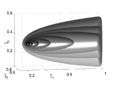
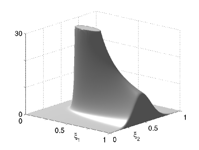
Figure 1: Anisotropy of the Green’s function $G$ associated with (1.1) for $\varepsilon=0.01$ and $\boldsymbol{x}=(\frac{1}{5},\frac{1}{2},\frac{1}{3})$. Left: isosurfaces at values of $1,\,4,\,8,\,16,\,32,\,64,\,128$, and $256$. Right: a two-dimensional graph for fixed $\xi_{3}=x_{3}$.

Our interest in considering the Green’s function of problem (1.1) and estimating its derivatives is motivated by the numerical analysis of this computationally challenging problem. More specifically, we shall use the obtained estimates in the forthcoming paper [6] to derive robust a posteriori error bounds for computed solutions of this problem using finite-difference methods. (This approach is related to recent articles [16, 3], which address the numerical solution of singularly perturbed equations of reaction-diffusion type.) In a more general numerical-analysis context, we note that sharp estimates for continuous Green’s functions (or their generalised versions) frequently play a crucial role in a priori and a posteriori error analyses [5, 11, 18].

The purpose of the present paper is to establish sharp bounds for the derivatives of the Green’s function in the $L_{1}$ norm (as they will be used to estimate the error in the computed solution in the dual $L_{\infty}$ norm [6]). Our estimates will be uniform in the small perturbation parameter $\varepsilon$ in the sense that any dependence on $\varepsilon$ will be shown explicitly. Note also that our estimates will be sharp (in the sense of Theorem 2.4) up to an $\varepsilon$-independent constant multiplier. We employ the analysis technique used in [8], which we now extend to a three-dimensional problem. Roughly speaking, we freeze the coefficients and estimate the corresponding explicit frozen-coefficient Green’s function, and then we investigate the difference between the original and the frozen-coefficient Green’s functions. This procedure is often called the parametrix method. To make this paper more readable, we deliberately follow some of the notation and presentation of [8].

The paper is organised as follows. In Section 2, the Green’s function associated with problem (1.1) is defined and upper bounds for its derivatives are stated in Theorem 2.2, the main result of the paper. The corresponding lower bounds are then given in Theorem 2.4. In Section 3, we obtain the fundamental solution for a constant-coefficient version of (1.1) in the domain $\Omega=\mathbb{R}^{3}$. This fundamental solution is bounded in Section 4. It is then used in Section 5 to construct certain approximations of the frozen-coefficient Green’s functions for the domains $\Omega=(0,1)\times\mathbb{R}^{2}$ and $\Omega=(0,1)^{3}$. The difference between these approximations and the original variable-coefficient Green’s function is estimated in Section 6, which completes the proof of Theorem 2.2.

Notation. Throughout the paper, $C$, as well as $c$, denotes a generic positive constant that may take different values in different formulas, but is independent of the small diffusion coefficient $\varepsilon$. A subscripted $C$ (e.g., $C_{1}$) denotes a positive constant that takes a fixed value, and is also independent of $\varepsilon$. The usual Sobolev spaces $W^{m,p}(D)$ and $L_{p}(D)$ on any measurable domain $D\subset\mathbb{R}^{3}$ are used. The $L_{p}(D)$-norm is denoted by $\|{\cdot}\|_{p\,;D}$ while the $W^{m,p}(D)$-norm is denoted by $\|{\cdot}\|_{m,p\,;D}$. By $\boldsymbol{x}=(x_{1},x_{2},x_{3})$ we denote an element in $\mathbb{R}^{3}$. For an open ball centred at $\boldsymbol{x^{\prime}}$ of radius $\rho$, we use the notation $B(\boldsymbol{x^{\prime}},\rho)=\{\boldsymbol{x}\in\mathbb{R}^{3}:\sum_{k=1,2,3}(x_{k}-x^{\prime}_{k})^{2}<\rho^{2}\}$. The notation $\partial_{x_{m}}f$, $\partial^{2}_{x_{m}}f$ and $\Delta_{\boldsymbol{x}}$ is employed for the first- and second-order partial derivatives of a function $f$ in variable $x_{m}$, and the Laplacian in variable $\boldsymbol{x}$, respectively, while $\partial^{2}_{x_{k}x_{m}}f$ will denote a mixed derivative of $f$.

2 Definition of Green’s function. Main result

The Green’s function $G=G(\boldsymbol{x};\boldsymbol{\xi})$ associated with (1.1), satisfies, for each fixed $\boldsymbol{x}\in\Omega$,

$$L^{*}_{\boldsymbol{\xi}}G(\boldsymbol{x};\boldsymbol{\xi}):=-\varepsilon\,\Delta_{\boldsymbol{\xi}}G+a(\boldsymbol{\xi})\,\partial_{\xi_{1}}G+b(\boldsymbol{\xi})\,G =\delta(\boldsymbol{x}-\boldsymbol{\xi}) \mbox{for}\;\boldsymbol{\xi}\in\Omega,$$ (2.1a)

$$G(\boldsymbol{x};\boldsymbol{\xi}) =0 \mbox{for}\;\boldsymbol{\xi}\in\partial\Omega.$$ (2.1b)

Here $L^{*}_{\boldsymbol{\xi}}$ is the adjoint differential operator to $L_{\boldsymbol{x}}$, and $\delta(\cdot)$ is the three-dimensional Dirac $\delta$-distribution. The unique solution $u$ of (1.1) allows the representation

$$u(\boldsymbol{x})=\iiint_{\Omega}G(\boldsymbol{x};\boldsymbol{\xi})\,f(\boldsymbol{\xi})\,d\boldsymbol{\xi}\,.$$ (2.2)

It should be noted that the Green’s function $G$ also satisfies, for each fixed $\boldsymbol{\xi}\in\Omega$,

$$L_{\boldsymbol{x}}G(\boldsymbol{x};\boldsymbol{\xi})=-\varepsilon\,\Delta_{\boldsymbol{x}}G-\partial_{x_{1}}(a(\boldsymbol{x})\,G)+b(\boldsymbol{x})\,G =\delta(\boldsymbol{x}-\boldsymbol{\xi}) \mbox{for}\;\boldsymbol{x}\in\Omega,$$ (2.3a)

$$G(\boldsymbol{x};\boldsymbol{\xi}) =0 \mbox{for}\;\boldsymbol{x}\in\partial\Omega.$$ (2.3b)

Consequently, the unique solution $v$ of the adjoint problem

$$L^{*}_{\boldsymbol{x}}v(\boldsymbol{x})=-\varepsilon\,\Delta_{\boldsymbol{x}}v+b(\boldsymbol{x})\,\partial_{x_{1}}v+c(\boldsymbol{x})\,v =f(\boldsymbol{x})\quad\mbox{for}\;\boldsymbol{x}\in\Omega,$$ (2.4a)

$$v(\boldsymbol{x}) =0\hskip 28.45274pt\,\mbox{for}\;\boldsymbol{x}\in\partial\Omega,$$ (2.4b)

is given by

$$v(\boldsymbol{\xi})=\iiint_{\Omega}G(\boldsymbol{x};\boldsymbol{\xi})\,f(\boldsymbol{x})\,d\boldsymbol{x}\,.$$ (2.5)

We start with a preliminary result for $G$.

Lemma 2.1.

Under assumptions (1.2), the Green’s function $G$ associated with (1.1) satisfies

$$\iint_{(0,1)^{2}}\!|G(\boldsymbol{x};\boldsymbol{\xi})|\,d\xi_{2}\,d\xi_{3}\leq C,\qquad\quad\|G(\boldsymbol{x};\cdot)\|_{1\,;\Omega}\leq C,$$ (2.6)

where $C$ is some positive $\varepsilon$-independent constant.

Proof.

The first estimate of (2.6) is given in the proof of [4, Theorem 2.10] (see also [19, Theorem III.1.22] and [2] for similar two-dimensional results). The second desired estimate follows. ∎

We now state the main result of this paper.

Theorem 2.2.

The Green’s function $G$ associated with (1.1), (1.2) in the unit-cube domain $\Omega=(0,1)^{3}$ satisfies, for all $\boldsymbol{x}\in\Omega$, the following bounds

$$\|{\partial_{\xi_{1}}G(\boldsymbol{x};\cdot)}\|_{1;\Omega} \leq C(1+|\ln\varepsilon|),$$ (2.7a)

$$\|{\partial_{\xi_{k}}G(\boldsymbol{x};\cdot)}\|_{1;\Omega}+\|{\partial_{x_{k}}G(\boldsymbol{x};\cdot)}\|_{1;\Omega} \leq C\varepsilon^{-1/2},\quad k=2,\,3.$$ (2.7b)

Furthermore, for any ball $$B(\boldsymbol{x}^{\prime},\rho) \rho \boldsymbol{x}^{\prime}\in\bar{\Omega}$$ of radius centered at any , we have

$$\|{G(\boldsymbol{x};\cdot)}\|_{1,1;B(\boldsymbol{x}^{\prime},\rho)} \leq C\varepsilon^{-1}\rho,$$ (2.7c)

while for the ball $$B(\boldsymbol{x},\rho) \rho \boldsymbol{x}$$ of radius centered at we have

$$\|{\partial^{2}_{\xi_{1}}G(\boldsymbol{x};\cdot)}\|_{1;\Omega\setminus B(\boldsymbol{x},\rho)} \leq C\varepsilon^{-1}\ln(2+\varepsilon/\rho),$$ (2.7d)

$$\|{\partial^{2}_{\xi_{k}}G(\boldsymbol{x};\cdot)}\|_{1;\Omega\setminus B(\boldsymbol{x},\rho)} \leq C\varepsilon^{-1}(|\ln\varepsilon|+\ln(2+\varepsilon/\rho)),\quad k=2,\,3.$$ (2.7e)

Here $C$ is some positive $\varepsilon$-independent constant.

We devote the rest of the paper to the proof of this theorem, which will be completed in Section 6.

In view of the solution representation (2.2), Theorem 2.2 yields a number of a priori solution estimates for our original problem. E.g., the bounds (2.7a), (2.7b) immediately imply the following result.

Corollary 2.3.

Let $f(\boldsymbol{x})=\partial_{x_{1}}F_{1}(\boldsymbol{x})+\partial_{x_{2}}F_{2}(\boldsymbol{x})+\partial_{x_{3}}F_{3}(\boldsymbol{x})$ with $F_{1},\,F_{2},\,F_{3}\in L_{\infty}(\Omega)$. Then there exists a unique solution $u\in L_{\infty}(\Omega)$ of problem (1.1), (1.2), for which we have the bound

$$\|{u}\|_{\infty\,;\Omega}\leq C\bigl{[}\,(1+|\ln\varepsilon|)\,\|{F_{1}}\|_{\infty\,;\Omega}+\varepsilon^{-1/2}\,(\|{F_{2}}\|_{\infty\,;\Omega}+\|{F_{3}}\|_{\infty\,;\Omega})\,\bigr{]}.$$ (2.8)

It can be anticipated from an inspection of the bounds for an explicit fundamental solution in a constant-coefficient case (see Section 4) that the upper estimates of Theorem 2.2 are sharp. Indeed, one can prove the following result.

Theorem 2.4 ([9]).

Let $\varepsilon\in(0,c_{0}]$ for some sufficiently small positive $c_{0}$. Set $a(\boldsymbol{x}):=\alpha$ and $b(\boldsymbol{x}):=0$ in (1.1). Then the Green’s function $G$ associated with this problem in the unit cube $\Omega=(0,1)^{3}$ satisfies, for all $\boldsymbol{x}\in[\frac{1}{4},\frac{3}{4}]^{3}$, the following lower bounds:

$$\|{\partial_{\xi_{1}}G(\boldsymbol{x};\cdot)}\|_{1;\Omega} \geq c\,|\ln\varepsilon|,$$ (2.9a)

$$\|{\partial_{\xi_{k}}G(\boldsymbol{x};\cdot)}\|_{1;\Omega} \geq c\,\varepsilon^{-1/2},\,k=2,\,3.$$ (2.9b)

Furthermore, for any ball $$B(\boldsymbol{x};\rho) \rho\leq\frac{1}{8}$$ of radius , we have

$$\|{G(\boldsymbol{x};\cdot)}\|_{1,1;\Omega\cap B(\boldsymbol{x};\rho)} \geq\begin{cases}c\,\rho/\varepsilon,&\mbox{for~{}}\rho\leq 2\varepsilon,\\ c\,(\rho/\varepsilon)^{1/2},&\mbox{otherwise},\\ \end{cases}$$ (2.9c)

$$\|{\partial^{2}_{\xi_{1}}G(\boldsymbol{x};\cdot)}\|_{1;\Omega\setminus B(\boldsymbol{x};\rho)} \geq c\,\varepsilon^{-1}\ln(2+\varepsilon/\rho),\quad \mbox{for~{}}\rho\leq c_{1}\varepsilon,$$ (2.9d)

$$\|{\partial^{2}_{\xi_{k}}G(\boldsymbol{x};\cdot)}\|_{1;\Omega\setminus B(\boldsymbol{x};\rho)} \geq c\,\varepsilon^{-1}(\ln(2+\varepsilon/\rho)+|\ln\varepsilon|) \mbox{for~{}}\rho\leq{\textstyle\frac{1}{8}},\,k=2,\,3.$$ (2.9e)

Here $$c c_{1} \varepsilon$$ and are -independent positive constants.

3 Fundamental solution in the constant-coefficient case

In our analysis, we invoke the observation that constant-coefficient versions of the two problems (2.1) and (2.3) that we have for $G$, can be easily solved explicitly when posed in $\mathbb{R}^{3}$. So in this section we shall explicitly solve simplifications of (2.1) and (2.3). To get these simplifications, we employ the parametrix method and so freeze the coefficients in these problems by replacing $a(\boldsymbol{\xi})$ by $a(\boldsymbol{x})$ in (2.1), and replacing $a(\boldsymbol{x})$ by $a(\boldsymbol{\xi})$ in (2.3), and also setting $b:=0$; the frozen-coefficient versions of the operators $L^{*}_{\boldsymbol{\xi}}$ and $L_{\boldsymbol{x}}$ will be denoted by $\bar{L}^{*}_{\boldsymbol{\xi}}$ and $\widetilde{L}_{\boldsymbol{x}}$, respectively. Furthermore, we extend the resulting equations to $\mathbb{R}^{3}$ and denote their solutions by $\bar{g}$ and $\widetilde{g}$. So we get

$$\bar{L}^{*}_{\boldsymbol{\xi}}\,\bar{g}(\boldsymbol{x};\boldsymbol{\xi})=-\varepsilon\,\Delta_{\boldsymbol{\xi}}\bar{g}(\boldsymbol{x};\boldsymbol{\xi})+a(\boldsymbol{x})\,\partial_{\xi_{1}}\bar{g}(\boldsymbol{x};\boldsymbol{\xi}) =\delta(\boldsymbol{x}-\boldsymbol{\xi})\quad\mbox{for}\;\boldsymbol{\xi}\in\mathbb{R}^{3},$$ (3.1)

$$\widetilde{L}_{\boldsymbol{x}}\,\widetilde{g}(\boldsymbol{x};\boldsymbol{\xi})=-\varepsilon\,\Delta_{\boldsymbol{x}}\widetilde{g}(\boldsymbol{x};\boldsymbol{\xi})-a(\boldsymbol{\xi})\,\partial_{x_{1}}\widetilde{g}(\boldsymbol{x};\boldsymbol{\xi}) =\delta(\boldsymbol{x}-\boldsymbol{\xi})\quad\mbox{for}\;\boldsymbol{x}\in\mathbb{R}^{3}.$$ (3.2)

As $\boldsymbol{x}$ appears in (3.1) as a parameter, so the coefficient $a(\boldsymbol{x})$ in this equation is considered constant and we can solve the problem explicitly. Setting $q=\frac{1}{2}a(\boldsymbol{x})$ for fixed $\boldsymbol{x}\in(0,1)^{3}$ and $\bar{g}(\boldsymbol{x};\boldsymbol{\xi})=V(\boldsymbol{x};\boldsymbol{\xi})\,\mathrm{e}^{q\xi_{1}/\varepsilon}$ (see, e.g., [13]), one gets

$$-\varepsilon^{2}\Delta_{\boldsymbol{\xi}}V+q^{2}V =\varepsilon\,\mathrm{e}^{-q\xi_{1}/\varepsilon}\,\delta(\boldsymbol{x}-\boldsymbol{\xi})=\varepsilon\,\mathrm{e}^{-qx_{1}/\varepsilon}\,\delta(\boldsymbol{x}-\boldsymbol{\xi}).$$

As the fundamental solution for the operator $-\varepsilon^{2}\Delta_{\boldsymbol{\xi}}+q^{2}$ is $\frac{1}{4\pi\varepsilon^{2}}\frac{\mathrm{e}^{-qr/\varepsilon}}{r}$ [21, Chapter VII], so

$$V(\boldsymbol{x};\boldsymbol{\xi})=\varepsilon\mathrm{e}^{-x_{1}q/\varepsilon}\frac{1}{4\pi\varepsilon^{2}}\frac{\mathrm{e}^{-rq/\varepsilon}}{r}\quad\mbox{where}\quad r=\sqrt{(x_{1}-\xi_{1})^{2}+(x_{2}-\xi_{2})^{2}+(x_{3}-\xi_{3})^{2}}.$$

Finally, for the solution of (3.1) we get

$$\bar{g}(\boldsymbol{x};\boldsymbol{\xi})=\frac{1}{4\pi\varepsilon^{2}}\,\frac{\mathrm{e}^{q(\xi_{1}-x_{1}-r)/\varepsilon}}{r},\qquad\mbox{where}\quad q=q(\boldsymbol{x})={\textstyle\frac{1}{2}}a(\boldsymbol{x}).$$

A similar argument yields the solution of (3.2)

$$\widetilde{g}(\boldsymbol{x};\boldsymbol{\xi})=\frac{1}{4\pi\varepsilon^{2}}\,\frac{\mathrm{e}^{q(\xi_{1}-x_{1}-r)/\varepsilon}}{r},\qquad\mbox{where}\quad q=q(\boldsymbol{\xi})={\textstyle\frac{1}{2}}a(\boldsymbol{\xi}).$$

Let $\widehat{\xi}_{1,[x_{1}]}=(\xi_{1}-x_{1})/\varepsilon$, $\widehat{\xi}_{2}=(\xi_{2}-x_{2})/\varepsilon$, $\widehat{\xi}_{3}=(\xi_{3}-x_{3})/\varepsilon$ and $\widehat{r}_{[x_{1}]}=\sqrt{\widehat{\xi}_{1,[x_{1}]}^{2}+\widehat{\xi}_{2}^{2}+\widehat{\xi}_{3}^{2}}$. As we shall need bounds for both $\bar{g}$ and $\widetilde{g}$, it is convenient to represent them via a more general function

$$g=g(\boldsymbol{x};\boldsymbol{\xi};q):=\frac{1}{4\pi\varepsilon^{2}}\,\frac{\mathrm{e}^{q(\widehat{\xi}_{1,[x_{1}]}-\widehat{r}_{[x_{1}]})}}{\widehat{r}_{[x_{1}]}}$$ (3.3)

as

$$\bar{g}(\boldsymbol{x};\boldsymbol{\xi})=g(\boldsymbol{x};\boldsymbol{\xi};q)\Bigr{|}_{q={\textstyle\frac{1}{2}}a(\boldsymbol{x})},\qquad\widetilde{g}(\boldsymbol{x};\boldsymbol{\xi})=g(\boldsymbol{x};\boldsymbol{\xi};q)\Bigr{|}_{q={\textstyle\frac{1}{2}}a(\boldsymbol{\xi})}$$ (3.4)

We use the subindex $[x_{1}]$ in $\widehat{\xi}_{1,[x_{1}]}$ and $\widehat{r}_{[x_{1}]}$ to highlight their dependence on $x_{1}$ as in many places $x_{1}$ will take different values; but when there is no ambiguity, we shall sometimes simply write $\widehat{\xi}_{1}$ and $\widehat{r}$.

4 Bounds for the fundamental solution $g(\boldsymbol{x};\boldsymbol{\xi};q)$

Throughout this section we assume that $\Omega=(0,1)\times\mathbb{R}^{2}$, but all results remain valid for $\Omega=(0,1)^{3}$. Here we derive a number of useful bounds for the fundamental solution $g$ of (3.3) and its derivatives that will be used in Section 5. As in $\bar{g}$ and $\widetilde{g}$ we set $q=\frac{1}{2}a(\boldsymbol{x})$ and $q=\frac{1}{2}a(\boldsymbol{\xi})$, respectively, so we shall also use, for $k=2,3$, the differential operators

$$D_{\xi_{k}}:=\partial_{\xi_{k}}+{\textstyle\frac{1}{2}}\partial_{\xi_{k}}a(\boldsymbol{\xi})\cdot\partial_{q},\qquad\quad D_{x_{k}}:=\partial_{x_{k}}+{\textstyle\frac{1}{2}}\partial_{x_{k}}a(\boldsymbol{x})\cdot\partial_{q}.$$ (4.1)

Lemma 4.1.

Let $\boldsymbol{x}\in[-1,1]\times\mathbb{R}^{2}$ and $0<\frac{1}{2}\alpha\leq q\leq C$. Then for the function $g=g(\boldsymbol{x};\boldsymbol{\xi};q)$ of (3.3) we have the following bounds

$$\|{g(\boldsymbol{x};\cdot;q)}\|_{1\,;\Omega} \leq C,$$ (4.2a)

$$\|{\partial_{\xi_{1}}g(\boldsymbol{x};\cdot;q)}\|_{1\,;\Omega} \leq C(1+|\ln\varepsilon|),$$ (4.2b)

$$\varepsilon^{1/2}\,\|{\partial_{\xi_{k}}g(\boldsymbol{x};\cdot;q)}\|_{1\,;\Omega}+\|{\partial_{q}g(\boldsymbol{x};\cdot;q)}\|_{1\,;\Omega} \leq C,\quad k=2,\,3,$$ (4.2c)

$$\|{(\varepsilon\widehat{r}_{[x_{1}]}\,\partial_{\xi_{1}}g)(\boldsymbol{x};\cdot;q)}\|_{1\,;\Omega} \leq C,$$ (4.2d)

$$\varepsilon^{1/2}\,\|{(\varepsilon\widehat{r}_{[x_{1}]}\,\partial^{2}_{\xi_{1}\xi_{k}}g)(\boldsymbol{x};\cdot;q)}\|_{1\,;\Omega}+\|{(\varepsilon\widehat{r}_{[x_{1}]}\,\partial^{2}_{\xi_{1}q}g)(\boldsymbol{x};\cdot;q)}\|_{1\,;\Omega} \leq C,\quad k=2,\,3,$$ (4.2e)

and for any ball $$B(\boldsymbol{x}^{\prime};\rho) \rho \boldsymbol{x}^{\prime}\in[0,1]\times\mathbb{R}^{2}$$ of radius centered at any , we have

$$\|{g(\boldsymbol{x};\cdot;q)}\|_{1,1\,;\Omega\cap B(\boldsymbol{x}^{\prime};\rho)} \leq C\varepsilon^{-1}\rho,$$ (4.2f)

while for the ball $$B(\boldsymbol{x};\rho) \rho \boldsymbol{x}$$ of radius centered at , we have

$$\|{\partial^{2}_{\xi_{1}}g(\boldsymbol{x};\cdot;q)}\|_{1\,;\Omega\setminus B(\boldsymbol{x};\rho)} \leq C\varepsilon^{-1}\ln(2+\varepsilon/\rho),$$ (4.2g)

$$\|{\partial^{2}_{\xi_{k}}g(\boldsymbol{x};\cdot;q)}\|_{1\,;\Omega\setminus B(\boldsymbol{x};\rho)} \leq C\varepsilon^{-1}(\ln(2+\varepsilon/\rho)+|\ln\varepsilon|),\quad k=2,\,3.$$ (4.2h)

Furthermore, one has the bound

$$\|{\partial_{x_{1}}g(\boldsymbol{x};\cdot;q)}\|_{1\,;\Omega}\leq C(1+|\ln\varepsilon|),$$ (4.3a)

and with the differential operators (4.1), one has, for $$k=2,\,3$$,

$$\|{D_{\xi_{k}}g(\boldsymbol{x};\cdot;q)}\|_{1\,;\Omega}+\|{D_{x_{k}}g(\boldsymbol{x};\cdot;q)}\|_{1\,;\Omega} \leq C\varepsilon^{-1/2},$$ (4.3b)

$$\|{(\varepsilon\widehat{r}_{[x_{1}]}\,D_{\xi_{k}}\partial_{x_{1}}g)(\boldsymbol{x};\cdot;q)}\|_{1\,;\Omega}+\|{(\varepsilon\widehat{r}_{[x_{1}]}\,D_{x_{k}}\partial_{\xi_{1}}g)(\boldsymbol{x};\cdot;q)}\|_{1\,;\Omega} \leq C\varepsilon^{-1/2}.$$ (4.3c)

Proof.

First, note that $\nabla_{\boldsymbol{x}}g=-\nabla_{\boldsymbol{\xi}}g$, so (4.3a) follows from (4.2b), (4.3b) follows from (4.1), (4.2c), while (4.3c) follows from (4.1), (4.2e). Thus it suffices to establish the bounds (4.2).

Throughout this proof, whenever $k$ appears in any relation, it will be understood to be valid for $k=2,3$ (as all the bounds in (4.2) that involve $k$, are given for both $k=2,3$).

A calculation shows that the first-order derivatives of $g=g(\boldsymbol{x};\boldsymbol{\xi};q)$ are given by

$$\partial_{\xi_{1}}g =\frac{1}{4\pi\varepsilon^{3}}\,\widehat{r}^{-2}\,\Bigl{[}q(\widehat{r}-\widehat{\xi}_{1})-\frac{\widehat{\xi}_{1}}{\widehat{r}}\,\Bigr{]}\,\,\mathrm{e}^{q(\widehat{\xi}_{1}-\widehat{r})},$$ (4.4a)

$$\partial_{\xi_{k}}g =-\frac{1}{4\pi\varepsilon^{3}}\,\bigl{(}q\widehat{r}+1\bigr{)}\,\frac{\widehat{\xi}_{k}}{\widehat{r}^{3}}\,\,\mathrm{e}^{q(\widehat{\xi}_{1}-\widehat{r})},$$ (4.4b)

$$\partial_{q}g =\frac{1}{4\pi\varepsilon^{2}}\,\frac{\widehat{\xi}_{1}-\widehat{r}}{\widehat{r}}\,\,\mathrm{e}^{q(\widehat{\xi}_{1}-\widehat{r})}.$$ (4.4c)

Here we used $\partial_{\xi_{j}}\widehat{r}=\varepsilon^{-1}\widehat{\xi}_{j}/\widehat{r}\,$ for $j=1,\,2,\,3$. In a similar manner, but also using $\partial_{\xi_{i}}(\widehat{\xi}_{j}/\widehat{r})=-\varepsilon^{-1}\widehat{\xi}_{i}\widehat{\xi}_{j}/\widehat{r}^{3}$ with $i\neq j$, one gets second-order derivatives

$$\partial^{2}_{\xi_{1}\xi_{k}}g =\frac{1}{4\pi\varepsilon^{4}}\,\frac{\widehat{\xi}_{k}}{\widehat{r}^{3}}\,\Bigl{[}q^{2}(\widehat{\xi}_{1}-\widehat{r})+q\frac{3\widehat{\xi}_{1}-\widehat{r}}{\widehat{r}}+3\frac{\widehat{\xi}_{1}}{\widehat{r}^{2}}\,\Bigr{]}\,\,\mathrm{e}^{q(\widehat{\xi}_{1}-\widehat{r})},$$ (4.5a)

$$\partial^{2}_{\xi_{1}q}g =\frac{1}{4\pi\varepsilon^{3}}\,\widehat{r}^{-2}\,\Bigl{[}-q(\widehat{\xi}_{1}-\widehat{r})^{2}+\frac{\widehat{r}^{2}-\widehat{\xi}_{1}^{2}}{\widehat{r}}\,\Bigr{]}\,\,\mathrm{e}^{q(\widehat{\xi}_{1}-\widehat{r})},$$ (4.5b)

$$\partial^{2}_{\xi_{k}}g =\frac{1}{4\pi\varepsilon^{4}}\,\widehat{r}^{-3}\,\Bigl{[}q^{2}\widehat{\xi}_{k}^{2}+(q\widehat{r}+1)\frac{3\widehat{\xi}_{k}^{2}-\widehat{r}^{2}}{\widehat{r}^{2}}\,\Bigr{]}\,\,\mathrm{e}^{q(\widehat{\xi}_{1}-\widehat{r})}.$$ (4.5c)

Finally, combining $$\partial_{\xi_{1}}^{2}g=-\partial_{\xi_{2}}^{2}g-\partial_{\xi_{3}}^{2}g+\frac{2q}{\varepsilon}\,\partial_{\xi_{1}}g$$ with (4.4a) and (4.5c) yields

$$\partial^{2}_{\xi_{1}}g =\frac{1}{4\pi\varepsilon^{4}}\,\widehat{r}^{-3}\,\Bigl{[}q^{2}\bigl{(}\widehat{r}-\widehat{\xi}_{1}\bigr{)}^{2}-q\bigl{(}\widehat{r}-\widehat{\xi}_{1}\bigr{)}\Bigl{(}1+3\frac{\widehat{\xi}_{1}}{\widehat{r}}\Bigr{)}+\frac{3\widehat{\xi}_{1}^{2}-\widehat{r}^{2}}{\widehat{r}^{2}}\,\Bigr{]}\,\,\mathrm{e}^{q(\widehat{\xi}_{1}-\widehat{r})}.$$ (4.5d)

Now we proceed to estimating the above derivatives of $g$. Note that $d\boldsymbol{\xi}=\varepsilon^{3}d\widehat{\boldsymbol{\xi}}$, where $\widehat{\boldsymbol{\xi}}\in\widehat{\Omega}:=\varepsilon^{-1}(-x_{1},1-x_{1})\times\mathbb{R}^{2}\subset(-\infty,2/\varepsilon)\times\mathbb{R}^{2}$. Consider the two sub-domains

$$\widehat{\Omega}_{1}:=\bigl{\{}\;\widehat{\xi}_{1}<1+{\textstyle\frac{1}{2}}\widehat{r}\;\bigr{\}},\qquad\widehat{\Omega}_{2}:=\bigl{\{}\;\max\{\,1,{\textstyle\frac{1}{2}}\widehat{r}\,\}<\widehat{\xi}_{1}<2/\varepsilon\;\bigr{\}}.$$

As $\widehat{\Omega}\subset\widehat{\Omega}_{1}\cup\widehat{\Omega}_{2}$ for any $x_{1}\in[-1,1]$, it is convenient to consider integrals over these two sub-domains separately.

(i) Consider $\widehat{\boldsymbol{\xi}}\in\widehat{\Omega}_{1}$. Then $\widehat{\xi}_{1}\leq 1+\frac{1}{2}\widehat{r}$, so one gets

$$\varepsilon^{3}\bigl{[}(1+\widehat{r})(\varepsilon^{-1}|g|+|\partial_{\xi_{1}}g|+|\partial_{\xi_{k}}g|+|\partial_{q}g|+|\partial^{2}_{\xi_{1}q}g|) +\varepsilon\widehat{r}|\partial^{2}_{\xi_{1}\xi_{k}}g|\bigr{]}$$

$$\leq C\,\widehat{r}^{-2}\,(1+\widehat{r}+\widehat{r}^{2}+\widehat{r}^{3})\,\,\mathrm{e}^{q(\widehat{\xi}_{1}-\widehat{r})}$$

$$\leq C\,\widehat{r}^{-2}\,\,\mathrm{e}^{-q\widehat{r}/4},$$ (4.6)

where we combined $\mathrm{e}^{q\widehat{\xi}_{1}}\leq\mathrm{e}^{q(1+\widehat{r}/2)}$ with $(1+\widehat{r}+\widehat{r}^{2}+\widehat{r}^{3})\leq C\mathrm{e}^{q\widehat{r}/4}$. This immediately yields

$$\iiint_{\widehat{\Omega}_{1}}\!\bigl{[}(1+\widehat{r})(\varepsilon^{-1}|g|+|\partial_{\xi_{1}}g|+|\partial_{\xi_{k}}g|+|\partial_{q}g|+|\partial^{2}_{\xi_{1}q}g|)+\varepsilon\widehat{r}|\partial^{2}_{\xi_{1}\xi_{k}}g|\bigr{]}\,\bigl{(}\varepsilon^{3}d\widehat{\boldsymbol{\xi}}\bigr{)}\\ \leq C\int_{0}^{\infty}\mathrm{e}^{-q\widehat{r}/4}\,d\widehat{r}\leq C.$$ (4.7)

Similarly,

$$\varepsilon^{3}\bigl{[}|\partial^{2}_{\xi_{1}}g|+|\partial^{2}_{\xi_{k}}g|\bigr{]}\leq C\varepsilon^{-1}\,\widehat{r}^{-3}\,(1+\widehat{r}^{2})\,\,\mathrm{e}^{q(\widehat{\xi}_{1}-\widehat{r})}\leq C\varepsilon^{-1}\,\widehat{r}^{-2}\,(\widehat{r}^{-1}+\widehat{r})\,\,\mathrm{e}^{-q\widehat{r}/2},$$

so

$$\iiint_{\widehat{\Omega}_{1}\setminus B(\boldsymbol{0};\widehat{\rho})}\!\bigl{[}|\partial^{2}_{\xi_{1}}g|+|\partial^{2}_{\xi_{k}}g|\bigr{]}\,\bigl{(}\varepsilon^{3}d\widehat{\boldsymbol{\xi}}\bigr{)}\leq C\varepsilon^{-1}\!\int_{\widehat{\rho}}^{\infty}\!\!(\widehat{r}^{-1}+\widehat{r})\,\mathrm{e}^{-q\widehat{r}/2}\,d\widehat{r}\leq C\varepsilon^{-1}\ln(2+\widehat{\rho}^{-1}).$$ (4.8)

Furthermore, for an arbitrary ball $\widehat{B}_{\widehat{\rho}}$ of radius $\widehat{\rho}$ in the coordinates $\boldsymbol{\widehat{\xi}}$, we get

$$\iiint_{\widehat{\Omega}_{1}\cap\widehat{B}_{\widehat{\rho}}}\!\bigl{[}|g|+|\partial_{\xi_{1}}g|+|\partial_{\xi_{k}}g|\bigr{]}\,\bigl{(}\varepsilon^{3}d\widehat{\boldsymbol{\xi}}\bigr{)}\leq C\int_{0}^{\widehat{\rho}}\!\!\mathrm{e}^{-q\widehat{r}/4}\,d\widehat{r}\leq C\min\{\widehat{\rho},1\}.$$ (4.9)

(ii) Next consider $\widehat{\boldsymbol{\xi}}\in\widehat{\Omega}_{2}$. In this sub-domain, it is convenient to rewrite the integrals in terms of $(\widehat{\xi}_{1},t_{2},t_{3})$, where

$$t_{k}:=\widehat{\xi}_{1}^{-1/2}\,\widehat{\xi}_{k},\quad\mbox{so}\quad\widehat{\xi}_{1}^{-1/2}\,d\widehat{\xi}_{k}=dt_{k}\quad\mbox{and}\quad\widehat{r}-\widehat{\xi}_{1}=\frac{\widehat{\xi}_{2}^{2}+\widehat{\xi}_{3}^{2}}{\widehat{r}+\widehat{\xi}_{1}}\leq t_{2}^{2}+t_{3}^{2}=:t^{2}.$$ (4.10)

Note that $\widehat{\xi}_{1}\leq\widehat{r}\leq 2\,\widehat{\xi}_{1}$ in $\widehat{\Omega}_{2}$ so $\widehat{r}-\widehat{\xi}_{1}=(\widehat{\xi}_{2}^{2}+\widehat{\xi}_{3}^{2})/(\widehat{r}+\widehat{\xi}_{1})\geq c_{0}t^{2}$, where $c_{0}:=\frac{1}{3}$. Consequently $\mathrm{e}^{-q(\widehat{r}-\widehat{\xi}_{1})}\leq\mathrm{e}^{-qc_{0}t^{2}}$ or

$$\mathrm{e}^{-q(\widehat{r}-\widehat{\xi}_{1})}\leq C\,\widehat{r}\,Q,\qquad\mbox{where}\quad Q:=\widehat{\xi}_{1}^{-1}\,\mathrm{e}^{-qc_{0}t^{2}},$$ (4.11)

and

$$\iint_{\mathbb{R}^{2}}(1+t+t^{2}+t^{3}+t^{4})\,Q\,\,d\widehat{\xi}_{2}\,d\widehat{\xi}_{3} =\iint_{\mathbb{R}^{2}}(1+t+t^{2}+t^{3}+t^{4})\,\mathrm{e}^{-qc_{0}t^{2}}\,dt_{2}\,dt_{3}$$

$$\leq C.$$ (4.12)

Using (4.4),(4.5) and (4.10) it is straightforward to prove the following bounds for $g$ and its derivatives in $\widehat{\Omega}_{2}$

$$\varepsilon^{3}|g| \leq C\,\varepsilon\,Q,$$ (4.13a)

$$\varepsilon^{3}|\partial_{\xi_{k}}g| \leq C\,\widehat{\xi}_{1}^{-1/2}\,t\,Q,$$ (4.13b)

$$\varepsilon^{3}|\partial^{2}_{\xi_{k}}g| \leq C\,\varepsilon^{-1}\,\widehat{\xi}_{1}^{-1}\,[1+t^{2}]\,Q,$$ (4.13c)

and also

$$\varepsilon^{3}(\varepsilon\widehat{r}|\partial_{\xi_{1}}g|+|\partial_{q}g|) \leq C\,\varepsilon\,[1+t^{2}]\,Q,$$ (4.13d)

$$\varepsilon^{3}|\partial_{\xi_{1}}g| \leq C\,\widehat{\xi}_{1}^{-1}\,[1+t^{2}]\,Q,$$ (4.13e)

$$\varepsilon^{3}(\varepsilon\widehat{r}|\partial_{\xi_{1}\xi_{k}}g|) \leq C\,\widehat{\xi}_{1}^{-1/2}\,t\,[1+t^{2}]\,Q,$$ (4.13f)

$$\varepsilon^{3}(\varepsilon\widehat{r}|\partial^{2}_{\xi_{1}q}g|) \leq C\,\varepsilon\,(t^{2}+t^{4})\,Q,$$ (4.13g)

$$\varepsilon^{3}|\partial^{2}_{\xi_{1}}g| \leq C\,\varepsilon^{-1}\,\widehat{\xi}_{1}^{-2}\,(1+t^{2}+t^{4})\,Q.$$ (4.13h)

Combining the obtained estimates (4.13) with (4.12) yields

$$\iiint_{\widehat{\Omega}_{2}}\!\bigl{[}|g|+\varepsilon^{1/2}|\partial_{\xi_{k}}g|+\varepsilon\widehat{r}|\partial_{\xi_{1}}g|+|\partial_{q}g| +\varepsilon^{1/2}\varepsilon\widehat{r}|\partial^{2}_{\xi_{1}\xi_{k}}g|+\varepsilon\widehat{r}|\partial^{2}_{\xi_{1}q}g|+|\partial_{\xi_{1}}^{2}g|\bigr{]}\,\bigl{(}\varepsilon^{3}d\widehat{\boldsymbol{\xi}}\bigr{)}$$

$$\leq C\int_{1}^{2/\varepsilon}\!\![\varepsilon+\varepsilon^{1/2}\widehat{\xi}_{1}^{-1/2}]\,d\widehat{\xi}_{1}\leq C.$$ (4.14)

Similarly, combining (4.13c) and (4.13e) with (4.12) yields

$$\iiint_{\widehat{\Omega}_{2}}\!\bigl{[}|\partial_{\xi_{1}}g|+\varepsilon|\partial^{2}_{\xi_{k}}g|\bigr{]}\,\bigl{(}\varepsilon^{3}d\widehat{\boldsymbol{\xi}}\bigr{)}\leq C\int_{1}^{2/\varepsilon}\!\!\widehat{\xi}_{1}^{-1}\,d\widehat{\xi}_{1}\leq C(1+|\ln\varepsilon|).$$ (4.15)

Furthermore, by (4.13b), and (4.13e) for an arbitrary ball $\widehat{B}_{\widehat{\rho}}$ of radius $\widehat{\rho}$ in the coordinates $\widehat{\boldsymbol{\xi}}$, we get

$$\iiint_{\widehat{\Omega}_{2}\cap\widehat{B}_{\widehat{\rho}}}\!(|g|+|\partial_{\xi_{1}}g|+|\partial_{\xi_{k}}g|)\,\bigl{(}\varepsilon^{3}d\widehat{\boldsymbol{\xi}}\bigr{)}\leq C\int_{1}^{1+\widehat{\rho}}\!\!\bigl{[}\varepsilon+\widehat{\xi}_{1}^{-1}+\widehat{\xi}_{1}^{-1/2}\bigr{]}\,d\widehat{\xi}_{1}\leq C\widehat{\rho}.$$ (4.16)

To complete the proof, we now recall that $\widehat{\Omega}\subset\widehat{\Omega}_{1}\cup\widehat{\Omega}_{2}$ and combine estimates (4.7) and (4.8) (that involve integration over $\widehat{\Omega}_{1}$) with (4.14) and (4.15), which yields the desired bounds (4.2a)-(4.2e) and (4.2g), (4.2h). To get the latter two bound we also used the observation that the ball $B(\boldsymbol{x};\rho)$ of radius $\rho$ in the coordinates $\boldsymbol{\xi}$ becomes the ball $B(\boldsymbol{0};\widehat{\rho})$ of radius $\widehat{\rho}=\varepsilon^{-1}\rho$ in the coordinates $\widehat{\boldsymbol{\xi}}$. The remaining assertion (4.2f) is obtained by combining (4.9) with (4.16) and noting that an arbitrary ball $B(\boldsymbol{x}^{\prime};\rho)$ of radius $\rho$ in the coordinates $\boldsymbol{\xi}$ becomes a ball $\widehat{B}_{\widehat{\rho}}$ of radius $\widehat{\rho}=\varepsilon^{-1}\rho$ in the coordinates $\widehat{\boldsymbol{\xi}}$. ∎

Our next result shows that for $x_{1}\geq 1$, one gets stronger bounds for $g$ and its derivatives. These bounds involve the weight function

$$\lambda:=\mathrm{e}^{2q(x_{1}-1)/\varepsilon}.$$ (4.17)

and show that, although $\lambda$ is exponentially large in $\varepsilon$, this is compensated by the smallness of $g$ and its derivatives.

Lemma 4.2.

Let $\boldsymbol{x}\in[1,3]\times\mathbb{R}^{2}$ and $0<\frac{1}{2}\alpha\leq q\leq C$. Then for the function $g=g(\boldsymbol{x};\boldsymbol{\xi};q)$ of (3.3) and the weight $\lambda$ of (4.17), one has the following bounds

$$\|{([1+\varepsilon\widehat{r}_{[x_{1}]}]\,\lambda g)(\boldsymbol{x};\cdot;q)}\|_{1\,;\Omega} \leq C\varepsilon,$$ (4.18a)

$$\|{(\lambda\,\partial_{\xi_{1}}g)(\boldsymbol{x};\cdot;q)}\|_{1\,;\Omega}+\|{(\lambda\,\partial_{q}g)(\boldsymbol{x};\cdot;q)}\|_{1\,;\Omega} \leq C,$$ (4.18b)

$$\|{([1+\varepsilon^{1/2}\widehat{r}_{[x_{1}]}]\,\lambda\,\partial_{\xi_{k}}g)(\boldsymbol{x};\cdot;q)}\|_{1\,;\Omega}+\varepsilon^{1/2}\|{(\varepsilon\widehat{r}_{[x_{1}]}\,\lambda\,\partial_{\xi_{1}\xi_{k}}^{2}g)(\boldsymbol{x};\cdot;q)}\|_{1\,;\Omega} \leq C,\quad k=2,3,$$ (4.18c)

$$\|{\widehat{r}_{[x_{1}]}\,\partial_{q}(\lambda\,g)(\boldsymbol{x};\cdot;q)}\|_{1\,;\Omega}+\|{\varepsilon\widehat{r}_{[x_{1}]}\,\partial_{q}(\lambda\,\partial_{\xi_{1}}g)(\boldsymbol{x};\cdot;q)}\|_{1\,;\Omega} \leq C,$$ (4.18d)

and for any ball $$B(\boldsymbol{x}^{\prime};\rho) \rho \boldsymbol{x}^{\prime}\in[0,1]\times\mathbb{R}^{2}$$ of radius centered at any , one has

$$\|{(\lambda\,g)(\boldsymbol{x};\cdot;q)}\|_{1,1\,;\Omega\cap B(\boldsymbol{x}^{\prime};\rho)} \leq C\varepsilon^{-1}\rho,$$ (4.18e)

while for the ball $$B(\boldsymbol{x};\rho) \rho \boldsymbol{x} k=1,\,2,\,3$$ of radius centered at and , one has

$$\|{(\lambda\,\partial^{2}_{\xi_{k}}g)(\boldsymbol{x};\cdot;q)}\|_{1\,;\Omega\setminus B(\boldsymbol{x},\rho)}\leq C\varepsilon^{-1}\ln(2+\varepsilon/\rho).$$ (4.18f)

Furthermore, with the differential operators (4.1) and $k=2,\,3$, we have

$$\|{\partial_{x_{1}}(\lambda g)(\boldsymbol{x};\cdot;q)}\|_{1\,;\Omega}+\|{D_{x_{k}}(\lambda g)(\boldsymbol{x};\cdot;q)}\|_{1\,;\Omega}+\|{D_{\xi_{k}}(\lambda g)(\boldsymbol{x};\cdot;q)}\|_{1\,;\Omega} \leq C,$$ (4.19a)

$$\|{\varepsilon\widehat{r}_{[x_{1}]}\,D_{x_{k}}(\lambda\,\partial_{\xi_{1}}g)(\boldsymbol{x};\cdot;q)}\|_{1\,;\Omega}+\|{\varepsilon\widehat{r}_{[x_{1}]}\,D_{\xi_{k}}\partial_{x_{1}}(\lambda g)(\boldsymbol{x};\cdot;q)}\|_{1\,;\Omega} \leq C\varepsilon^{-1/2}.$$ (4.19b)

Proof.

Throughout this proof, whenever $k$ appears in any relation, it will be understood to be valid for $k=2,3$ (as all the bounds in (4.18), (4.19) that involve $k$, are given for both $k=2,3$).

We shall use the notation $A=A(x_{1}):=(x_{1}-1)/\varepsilon\geq 0$. Then (4.17) becomes $\lambda=\mathrm{e}^{2qA}$. We partially imitate the proof of Lemma 4.1. Again $d\boldsymbol{\xi}=\varepsilon^{3}\,d\widehat{\boldsymbol{\xi}}$, but now $\widehat{\boldsymbol{\xi}}\in\widehat{\Omega}=\varepsilon^{-1}(-x_{1},1-x_{1})\times\mathbb{R}^{2}\subset(-3/\varepsilon,-A)\times\mathbb{R}^{2}$. So $\widehat{\xi}_{1}<-A\leq 0$ immediately yields

$$\lambda\,\mathrm{e}^{q\widehat{\xi}_{1}}=\mathrm{e}^{2q(A-|\widehat{\xi}_{1}|)}\,\mathrm{e}^{q|\widehat{\xi}_{1}|}\leq\mathrm{e}^{q|\widehat{\xi}_{1}|}.$$ (4.20)

Consider the sub-domains

$$\widehat{\Omega}^{\prime}_{1} :=\bigl{\{}\;|\widehat{\xi}_{1}|<1+{\textstyle\frac{1}{2}\widehat{r}},\;\;\widehat{\xi}_{1}<-A\;\bigr{\}},$$

$$\widehat{\Omega}^{\prime}_{2} :=\bigl{\{}\;|\widehat{\xi}_{1}|>\max\{\textstyle 1,{\textstyle\frac{1}{2}\widehat{r}}\},\;\;-3/\varepsilon<\widehat{\xi}_{1}<-A\;\bigr{\}}.$$

As $\widehat{\Omega}\subset\widehat{\Omega}_{1}^{\prime}\cup\widehat{\Omega}_{2}^{\prime}$ for any $x_{1}\in[1,3]$, we estimate integrals over these two domains separately.

(i) Let $\widehat{\boldsymbol{\xi}}\in\widehat{\Omega}^{\prime}_{1}$. Then $|\widehat{\xi}_{1}|\leq 1+\frac{1}{2}\widehat{r}$ so, by (4.20), one has $\lambda\,\mathrm{e}^{q\widehat{\xi}_{1}}\leq\mathrm{e}^{q(1+\widehat{r}/2)}$. The first inequality in (4.6) remains valid, but now we combine it with

$$\lambda\,\mathrm{e}^{q(\widehat{\xi}_{1}-\widehat{r})}\,(1+\widehat{r}+\widehat{r}^{2}+\widehat{r}^{3})\,\leq C\,\mathrm{e}^{-q\widehat{r}/4}$$ (4.21)

(which is obtained similarly to the final line in (4.6)). This leads to a version of (4.7) that involves the weight $\lambda$:

$$\iiint_{\widehat{\Omega}_{1}^{\prime}}\lambda\,\bigl{[}(1+\widehat{r})(\varepsilon^{-1}|g|+|\partial_{\xi_{1}}g|+|\partial_{\xi_{k}}g|+\varepsilon^{-1}|\partial_{q}g|+|\partial^{2}_{\xi_{1}q}g|)+\varepsilon\widehat{r}|\partial^{2}_{\xi_{1}\xi_{k}}g|\bigr{]}\,\bigl{(}\varepsilon^{3}d\widehat{\boldsymbol{\xi}}\bigr{)}\leq C.$$ (4.22)

In a similar manner, we obtain versions of estimates (4.8) and (4.9), that also involve the weight $\lambda$:

$$\iiint_{\widehat{\Omega}_{1}^{\prime}\setminus B(\boldsymbol{0};\widehat{\rho})}\!\lambda\,|\partial^{2}_{\xi_{k}}g|\,\bigl{(}\varepsilon^{3}d\widehat{\boldsymbol{\xi}}\bigr{)}\leq C\varepsilon^{-1}\ln(2+\widehat{\rho}^{-1}),$$ (4.23)

$$\iiint_{\widehat{\Omega}_{1}^{\prime}\cap\widehat{B}_{\widehat{\rho}}}\!\lambda\bigl{[}|g|+|\partial_{\xi_{1}}g|+|\partial_{\xi_{k}}g|\bigr{]}\,\bigl{(}\varepsilon^{3}d\widehat{\boldsymbol{\xi}}\bigr{)}\leq C\min\{\widehat{\rho},1\},$$ (4.24)

where $\widehat{B}_{\widehat{\rho}}$ is an arbitrary ball of radius $\widehat{\rho}$ in the coordinates $\widehat{\boldsymbol{\xi}}$. Furthermore, (4.22) combined with $|\partial_{q}(\lambda\,g)|\leq\lambda(2A|g|+|\partial_{q}g|)$ and $|\partial_{q}(\lambda\,\partial_{\xi_{1}}g)|\leq\lambda(2A|\partial_{\xi_{1}}g|+|\partial^{2}_{\xi_{1}q}g|)$ and then with $A\leq 2/\varepsilon$ yields

$$\iiint_{\widehat{\Omega}_{1}^{\prime}}\,\widehat{r}\,\bigl{[}|\partial_{q}(\lambda\,g)|+\varepsilon|\partial_{q}(\lambda\,\partial_{\xi_{1}}g)|\bigr{]}\,\bigl{(}\varepsilon^{3}d\widehat{\boldsymbol{\xi}}\bigr{)}\leq C.$$ (4.25)

(ii) Now consider $\widehat{\boldsymbol{\xi}}\in\widehat{\Omega}^{\prime}_{2}$. In this sub-domain (similarly to $\widehat{\Omega}_{2}$ in the proof of Lemma 4.1) one has $|\widehat{\xi}_{1}|\leq\widehat{r}\leq 2|\widehat{\xi}_{1}|$ and $c_{0}t^{2}\leq\widehat{r}-|\widehat{\xi}_{1}|\leq t^{2}$, where $t_{k}:=|\widehat{\xi}_{1}|^{-1/2}\,\widehat{\xi}_{k}$ for $k=2,3$, and $t^{2}:=t_{2}^{2}+t_{3}^{2}$, (compare with (4.10)). We also introduce a new barrier $Q$

$$Q:=\lambda^{-1}\,\mathrm{e}^{2q(A-|\widehat{\xi}_{1}|)}\,\bigl{\{}|\widehat{\xi}_{1}|^{-1}\,\mathrm{e}^{-qc_{0}t^{2}}\bigr{\}}\qquad\Rightarrow\quad\mathrm{e}^{-q(\widehat{r}-\widehat{\xi}_{1})}\leq C\,\widehat{r}\,Q,$$ (4.26)

(compare with (4.11); to get the bound for $\mathrm{e}^{-q(\widehat{r}-\widehat{\xi}_{1})}$ we used (4.20)).

With the new definition (4.26) of $Q$, the bounds (4.13a)–(4.13c) remain valid in $\widehat{\Omega}_{2}^{\prime}$ only with $\widehat{\xi}_{1}$ replaced by $|\widehat{\xi}_{1}|$. Note that the bounds (4.13d)–(4.13g) are not valid in $\widehat{\Omega}_{2}^{\prime}$, (as they were obtained using $\widehat{r}-\widehat{\xi}_{1}\leq t^{2}$, which is not the case for $\widehat{\xi}_{1}<0$). Instead, using $\widehat{r}\geq|\widehat{\xi}_{1}|\geq 1$ and $\widehat{r}\leq 2|\widehat{\xi}_{1}|$, we prove, directly from (4.4),(4.5), the following bounds in $\widehat{\Omega}^{\prime}_{2}$:

$$\varepsilon^{3}|\partial_{\xi_{1}}g| \leq C\,Q,$$ (4.27a)

$$\varepsilon^{3}|\partial_{q}g| \leq C\,\varepsilon|\widehat{\xi}_{1}|\,Q,$$ (4.27b)

$$\varepsilon^{3}(\varepsilon\widehat{r}|\partial_{\xi_{1}\xi_{k}}g|) \leq C\,|\widehat{\xi}_{1}|^{1/2}\,t\,Q,$$ (4.27c)

$$\varepsilon^{3}(|\partial_{q}(\lambda\,g)|+\varepsilon|\partial_{q}(\lambda\,\partial_{\xi_{1}}g)|) \leq C\,\varepsilon\lambda\,[(|\widehat{\xi}_{1}|-A)+t^{2}+1]\,Q.$$ (4.27d)

In particular, to establish (4.27d), we combined $\partial_{q}(\lambda\,g)=\lambda[2A\,g+\partial_{q}g]$ and $\partial_{q}(\lambda\,\partial_{\xi_{1}}g)=\lambda[2A\,\partial_{\xi_{1}}g+\partial^{2}_{\xi_{1}q}g]$ with the observations that

$$(\widehat{r}+|\widehat{\xi}_{1}|)-2A=2(|\widehat{\xi}_{1}|-A)+(\widehat{r}-|\widehat{\xi}_{1}|)\leq 2(|\widehat{\xi}_{1}|-A)+t^{2}$$

and $\widehat{r}^{-1}A\leq C$.

Next, note that (4.12) is valid with $Q$ replaced by the multiplier $\bigl{\{}|\widehat{\xi}_{1}|^{-1}\,\mathrm{e}^{-qc_{0}t^{2}}\bigr{\}}$ from the current definition (4.26) of $Q$. Combining this observation with the bounds (4.13a)–(4.13c) and (4.27a)–(4.27c), and also with $\widehat{r}\leq 2|\widehat{\xi}_{1}|$, yields

$$\iiint_{\widehat{\Omega}_{2}^{\prime}}\!\!\lambda\,\bigl{[} (\varepsilon^{-1}+\widehat{r})|g|+|\partial_{\xi_{1}}g|+(1+\varepsilon^{1/2}\widehat{r})|\partial_{\xi_{k}}g|+|\partial_{q}g|+\varepsilon^{1/2}(\varepsilon\widehat{r}|\partial^{2}_{\xi_{1}\xi_{k}}g|)+\varepsilon|\partial^{2}_{\xi_{k}}g|\bigr{]}\,\bigl{(}\varepsilon^{3}d\widehat{\boldsymbol{\xi}}\bigr{)}$$

$$\leq C\int_{-3/\varepsilon}^{-\max\{A,1\}}\!\bigl{[}1+\varepsilon|\widehat{\xi}_{1}|+|\widehat{\xi}_{1}|^{-1/2}+(\varepsilon|\widehat{\xi}_{1}|)^{1/2}+|\widehat{\xi}_{1}|^{-1}\bigr{]}\,\mathrm{e}^{2q(A-|\widehat{\xi}_{1}|)}\,d\widehat{\xi}_{1}\leq C.$$ (4.28)

Similarly, from (4.27d) combined with $\widehat{r}\leq 2|\widehat{\xi}_{1}|\leq 6\varepsilon^{-1}$, one gets

$$\iiint_{\widehat{\Omega}_{2}^{\prime}}\!\widehat{r}\bigl{[}|\partial_{q}(\lambda\,g)|+\varepsilon|\partial_{q}(\lambda\,\partial_{\xi_{1}}g)|\bigr{]}\,\bigl{(}\varepsilon^{3}d\widehat{\boldsymbol{\xi}}\bigr{)}\\ \leq C\int_{-3/\varepsilon}^{-\max\{A,1\}}\!\!\bigl{[}(|\widehat{\xi}_{1}|-A)+1\bigr{]}\,\mathrm{e}^{2q(A-|\widehat{\xi}_{1}|)}\,d\widehat{\xi}_{1}\leq C.$$ (4.29)

Furthermore, by (4.13b), and (4.27a), for an arbitrary ball $\widehat{B}_{\widehat{\rho}}$ of radius $\widehat{\rho}$ in the coordinates $\widehat{\boldsymbol{\xi}}$, we get

$$\iiint_{\widehat{\Omega}^{\prime}_{2}\cap\widehat{B}_{\widehat{\rho}}}\!\lambda\,[|g|+|\partial_{\xi_{1}}g|+|\partial_{\xi_{k}}g|]\,\bigl{(}\varepsilon^{3}d\widehat{\boldsymbol{\xi}}\bigr{)} \leq C\int^{-\max\{A,1\}}_{-\max\{A,1\}-\widehat{\rho}}\bigl{[}1+|\widehat{\xi}_{1}|^{-1/2}\bigr{]}\,\mathrm{e}^{2q(A-|\widehat{\xi}_{1}|)}d\widehat{\xi}_{1}$$

$$\leq C\widehat{\rho}.$$ (4.30)

To complete the proof of (4.18), we now recall that $\widehat{\Omega}\subset\widehat{\Omega}_{1}^{\prime}\cup\widehat{\Omega}_{2}^{\prime}$ and combine estimates (4.22), (4.23), (4.25) (that involve integration over $\widehat{\Omega}_{1}^{\prime}$) with (4.28), (4.29), which yields the desired bounds (4.18a)–(4.18d) and the bounds for $\partial_{\xi_{2}}^{2}g$ and $\partial_{\xi_{3}}^{2}g$ in (4.18f). To get the latter two bounds we also used the observation that the ball $B(\boldsymbol{x};\rho)$ of radius $\rho$ in the coordinates $\boldsymbol{\xi}$ becomes the ball $B(\boldsymbol{0};\widehat{\rho})$ of radius $\widehat{\rho}=\varepsilon^{-1}\rho$ in the coordinates $\widehat{\boldsymbol{\xi}}$. The bound for $\partial^{2}_{\xi_{1}}g$ in (4.18f) follows as $\partial^{2}_{\xi_{1}}g=-\partial^{2}_{\xi_{2}}g-\partial^{2}_{\xi_{3}}g+\frac{2q}{\varepsilon}\,\partial_{\xi_{1}}g$ for $\boldsymbol{\xi}\neq\boldsymbol{x}$. The remaining assertion (4.18e) is obtained by combining (4.24) with (4.30) and noting that an arbitrary ball $B(\boldsymbol{x}^{\prime};\rho)$ of radius $\rho$ in the coordinates $\boldsymbol{\xi}$ becomes a ball $\widehat{B}_{\widehat{\rho}}$ of radius $\widehat{\rho}=\varepsilon^{-1}\rho$ in the coordinates $\widehat{\boldsymbol{\xi}}$. Thus we have established all the bounds (4.18).

We now proceed to the proof of the bounds (4.19). Note that $\nabla_{\boldsymbol{x}}g=-\nabla_{\boldsymbol{\xi}}g$. Combining these with (4.18b) and the bounds for $\|{\lambda\,\partial_{\xi_{2}}g}\|_{1\,;\Omega}$ and $\|{\lambda\,\partial_{\xi_{3}}g}\|_{1\,;\Omega}$ in (4.18c), yields

$$\|{\lambda\,\partial_{x_{1}}g}\|_{1\,;\Omega}+\|{\lambda\,D_{x_{k}}g}\|_{1\,;\Omega}+\|{\lambda\,D_{\xi_{k}}g}\|_{1\,;\Omega}\leq C.$$

Now, combining $\partial_{x_{1}}\lambda=2q\varepsilon^{-1}\lambda$ and $\partial_{q}\lambda=2A\lambda\leq 4\varepsilon^{-1}\lambda$ with (4.18a), yields

$$\|{g\,\partial_{x_{1}}\lambda}\|_{1\,;\Omega}+\|{g\,D_{x_{k}}\lambda}\|_{1\,;\Omega}+\|{g\,D_{\xi_{k}}\lambda}\|_{1\,;\Omega}\leq C.$$

Consequently, we get (4.19a).

To estimate $\varepsilon\widehat{r}\,D_{x_{k}}(\lambda\,\partial_{\xi_{1}}g)$, note that it involves $\varepsilon\widehat{r}\,\partial_{x_{k}}(\lambda\,\partial_{\xi_{1}}g)=-\varepsilon\widehat{r}\,\lambda\,\partial^{2}_{\xi_{1}\xi_{k}}g$ for which we have a bound in (4.18c), and also $\varepsilon\widehat{r}\,\partial_{q}(\lambda\,\partial_{\xi_{1}}g)$, for which we have a bound in (4.18d). The desired bounds for $\varepsilon\widehat{r}\,D_{x_{k}}(\lambda\,\partial_{\xi_{1}}g)$ in (4.19b) follow.

For $\varepsilon\widehat{r}\,D_{\xi_{k}}\partial_{x_{1}}(\lambda g)$ in (4.19b), a calculation yields $\varepsilon\widehat{r}\,D_{\xi_{k}}\partial_{x_{1}}(\lambda g)=\varepsilon\widehat{r}\,D_{\xi_{k}}(\lambda\,\partial_{x_{1}}g)+2\widehat{r}\,D_{\xi_{k}}(q\lambda\,g)$. The first term is estimated similarly to $\varepsilon\widehat{r}\,D_{x_{k}}(\lambda\,\partial_{\xi_{1}}g)$ in (4.19b). The remaining term $\widehat{r}\,D_{\xi_{k}}(q\lambda\,g)$ involves $\widehat{r}\,\partial_{\xi_{k}}(q\lambda\,g)=q\,\widehat{r}\,\lambda\,\partial_{\xi_{k}}g$, for which we have a bound in (4.18c), and also $\widehat{r}\,\partial_{q}(q\lambda\,g)=q\,\widehat{r}\,\partial_{q}(\lambda\,g)+\widehat{r}\,\lambda\,g$, for which we have bounds in (4.18d) and (4.18a). Consequently (4.19b) is proved. ∎

Lemma 4.3.

Under the conditions of Lemma 4.2, for some positive constant $c_{1}$ one has

$$\|\lambda g(\boldsymbol{x};\cdot)\|_{2,1\,;[0\frac{1}{3}]\times\mathbb{R}^{2}}+\|D_{x_{k}}(\lambda g)(\boldsymbol{x};\cdot)\|_{1,1\,;[0\frac{1}{3}]\times\mathbb{R}^{2}}\leq C\mathrm{e}^{-c_{1}\alpha/\varepsilon},\quad k=2,\,3.$$ (4.31)

Proof.

We imitate the proof of Lemma 4.2, only now $\xi_{1}<\frac{1}{3}$ or $\widehat{\xi}_{1}<(\frac{1}{3}-x_{1})/\varepsilon\leq-\frac{2}{3}/\varepsilon$. Thus instead of the sub-domains $\widehat{\Omega}_{1}^{\prime}$ and $\widehat{\Omega}_{2}^{\prime}$ we now consider $\widehat{\Omega}_{1}^{\prime\prime}$ and $\widehat{\Omega}_{2}^{\prime\prime}$ defined by $\widehat{\Omega}_{k}^{\prime\prime}:=\widehat{\Omega}_{k}^{\prime}\cap\{\widehat{\xi}_{1}<-(x_{1}-\frac{1}{3})/\varepsilon\}$. Thus in $\widehat{\Omega}_{1}^{\prime\prime}$ (4.21) remains valid with $q\geq\frac{1}{2}\alpha$, but now $\widehat{r}>\frac{2}{3}/\varepsilon$. Therefore, when we integrate over $\widehat{\Omega}_{1}^{\prime\prime}$ (instead of $\widehat{\Omega}_{1}^{\prime}$), the integrals of type (4.22), (4.23) become bounded by $C\mathrm{e}^{-c_{1}\alpha/\varepsilon}$ for any fixed $c_{1}<\frac{1}{8}$. Next, when considering integrals over $\widehat{\Omega}_{2}^{\prime\prime}$ (instead of $\widehat{\Omega}_{2}^{\prime}$), note that $A-|\widehat{\xi}_{1}|\leq-\frac{2}{3}/\varepsilon$ so the quantity $\mathrm{e}^{2q(A-|\widehat{\xi}_{1}|)}$ in the definition (4.26) of $Q$ is now bounded by $\mathrm{e}^{-\frac{2}{3}\alpha/\varepsilon}$. Consequently, the integrals of type (4.28) over $\widehat{\Omega}_{2}^{\prime\prime}$ also become bounded by $C\mathrm{e}^{-c_{1}\alpha/\varepsilon}$. ∎

Remark 4.4.

The estimates of Lemmas 4.1 and 4.2 remain valid if we set $q:=\frac{1}{2}a(\boldsymbol{x})$ or $q:=\frac{1}{2}a(\boldsymbol{\xi})$ in $g$, $\lambda$, and their derivatives (after the differentiation is performed).

5 Approximations $\bar{G}$ and $\widetilde{G}$ for the Green’s function $G$

We shall use two related cut-off functions $\omega_{0}$ and $\omega_{1}$ defined by

$$\omega_{0}(t)\in C^{2}(0,1),\quad\omega_{0}(t)=1\;\mbox{for }t\leq{\textstyle\frac{2}{3}},\quad\omega_{0}(t)=0\;\mbox{for }t\geq{\textstyle\frac{5}{6}};\quad\omega_{1}(t):=\omega_{0}(1-t),$$ (5.1)

so $\omega_{m}(m)=1$, $\omega_{m}(1-m)=0$ and $\omega_{m}^{\prime}(t)\bigr{|}_{t=0,1}=\omega_{m}^{\prime\prime}(t)\bigr{|}_{t=0,1}=0$ for $m=0,1$.

Our purpose in this section is to introduce and estimate frozen-coefficient approximations $\bar{G}$ and $\widetilde{G}$ of $G$. We consider the domain $\Omega=(0,1)\times\mathbb{R}^{2}$ in the first part of this section, and the domain $\Omega=(0,1)^{3}$ in the second part. Note that although $\bar{G}$ and $\widetilde{G}$ will be constructed as solution approximations for the frozen-coefficient equations, we shall see in Section 6 that they, in fact, provide approximations to the Green’s function $G$ for our original variable-coefficient problem.

5.1 Approximations $\bar{G}$ and $\widetilde{G}$ in the domain $\Omega=(0,1)\times\mathbb{R}^{2}$

To construct approximations $\bar{G}$ and $\widetilde{G}$, we employ the method of images with an inclusion of the cut-off functions of (5.1). So, using the fundamental solution $g$ of (3.3), we define

$$\bar{G}(\boldsymbol{x};\boldsymbol{\xi}):=\bar{\mathcal{G}}\bigr{|}_{q=\frac{1}{2}a(\boldsymbol{x})},\qquad\widetilde{G}(\boldsymbol{x};\boldsymbol{\xi}):=\widetilde{\mathcal{G}}\bigr{|}_{q=\frac{1}{2}a(\boldsymbol{\xi})},$$ (5.2)

$$\bar{\mathcal{G}}(\boldsymbol{x};\boldsymbol{\xi};q) :=\frac{\mathrm{e}^{q\widehat{\xi}_{1,[x_{1}]}}}{4\pi\varepsilon^{2}}\left\{\left[\frac{\mathrm{e}^{-q\widehat{r}_{[x_{1}]}}}{\widehat{r}_{[x_{1}]}}-\frac{\mathrm{e}^{-q\widehat{r}_{[-x_{1}]}}}{\widehat{r}_{[-x_{1}]}}\right]-\left[\frac{\mathrm{e}^{-q\widehat{r}_{[2-x_{1}]}}}{\widehat{r}_{[2-x_{1}]}}-\frac{\mathrm{e}^{-q\widehat{r}_{[2+x_{1}]}}}{\widehat{r}_{[2+x_{1}]}}\right]\omega_{1}(\xi_{1})\right\},$$ (5.3a)

$$\widetilde{\mathcal{G}}(\boldsymbol{x};\boldsymbol{\xi};q) :=\frac{\mathrm{e}^{q\widehat{\xi}_{1,[x_{1}]}}}{4\pi\varepsilon^{2}}\left\{\left[\frac{\mathrm{e}^{-q\widehat{r}_{[x_{1}]}}}{\widehat{r}_{[x_{1}]}}-\frac{\mathrm{e}^{-q\widehat{r}_{[2-x_{1}]}}}{\widehat{r}_{[2-x_{1}]}}\right]-\left[\frac{\mathrm{e}^{-q\widehat{r}_{[-x_{1}]}}}{\widehat{r}_{[-x_{1}]}}-\frac{\mathrm{e}^{-q\widehat{r}_{[2+x_{1}]}}}{\widehat{r}_{[2+x_{1}]}}\right]\omega_{0}(x_{1})\right\}.$$ (5.3b)

Note that $\bar{G}\bigr{|}_{\xi_{1}=0,1}=0$ and $\widetilde{G}\bigr{|}_{x_{1}=0,1}=0$ (the former observation follows from $\widehat{r}_{[x_{1}]}=\widehat{r}_{[-x_{1}]}$ at $\xi_{1}=0$, and $\widehat{r}_{[x_{1}]}=\widehat{r}_{[2-x_{1}]}$ and $\widehat{r}_{[-x_{1}]}=\widehat{r}_{[2+x_{1}]}$ at $\xi_{1}=1$). We shall see shortly (see Lemma 5.1) that $\bar{L}^{*}_{\boldsymbol{\xi}}\bar{G}\approx L^{*}_{\boldsymbol{\xi}}G$ and $\widetilde{L}_{\boldsymbol{x}}\widetilde{G}\approx L_{\boldsymbol{x}}G$; in this sense $\bar{G}$ and $\widetilde{G}$ give approximations for $G$.

Rewrite the definitions of $\bar{\mathcal{G}}$ and $\widetilde{\mathcal{G}}$ using the notation

$$g_{[d]} :=g(d,x_{2},x_{3};\boldsymbol{\xi};q)={\frac{1}{4\pi\varepsilon^{2}}}\,\frac{\mathrm{e}^{q(\widehat{\xi}_{1,[d]}-\widehat{r}_{[d]})}}{\widehat{r}_{[d]}},$$ (5.4a)

$$\lambda^{\pm} :=\mathrm{e}^{2q(1\pm x_{1})/{\varepsilon}},\qquad\quad p:=\mathrm{e}^{-2qx_{1}/{\varepsilon}},$$ (5.4b)

and the observation that

$${\frac{1}{4\pi\varepsilon^{2}}}\,\frac{\mathrm{e}^{q(\widehat{\xi}_{1,[x_{1}]}-\widehat{r}_{[d]})}}{\widehat{r}_{[d]}}=\mathrm{e}^{q(d-x_{1})/\varepsilon}\,g_{[d]}\qquad\mbox{for}\;\;d=\pm x_{1},2\pm x_{1}.$$ (5.5)

They yield

$$\bar{\mathcal{G}}(\boldsymbol{x};\boldsymbol{\xi};q) =\left[g_{[x_{1}]}-p\,g_{[-x_{1}]}\right]-\left[\lambda^{-}g_{[2-x_{1}]}-p\,\lambda^{\!+}g_{[2+x_{1}]}\right]\omega_{1}(\xi_{1}),$$ (5.6a)

$$\widetilde{\mathcal{G}}(\boldsymbol{x};\boldsymbol{\xi};q) =\left[g_{[x_{1}]}-\lambda^{-}g_{[2-x_{1}]}\right]-\left[p\,g_{[-x_{1}]}-p\,\lambda^{\!+}g_{[2+x_{1}]}\right]\omega_{0}(x_{1}).$$ (5.6b)

Note that $\lambda^{\pm}$ is obtained by replacing $x_{1}$ by $2\pm x_{1}$ in the definition (4.17) of $\lambda$.

In the next lemma, we estimate the functions

$$\bar{\phi}(\boldsymbol{x};\boldsymbol{\xi}):=\bar{L}^{*}_{\boldsymbol{\xi}}\bar{G}-L^{*}_{\boldsymbol{\xi}}G,\qquad\widetilde{\phi}(\boldsymbol{x};\boldsymbol{\xi}):=\widetilde{L}_{\boldsymbol{x}}\widetilde{G}-L_{\boldsymbol{x}}G.$$ (5.7)

Lemma 5.1.

Let $\boldsymbol{x}\in\Omega=(0,1)\times\mathbb{R}^{2}$. Then for the functions $\bar{\phi}$ and $\widetilde{\phi}$ of (5.7), one has

$$\|\bar{\phi}(\boldsymbol{x};\cdot)\|_{1,1\,;\Omega}+\|\partial_{x_{2}}\bar{\phi}(\boldsymbol{x};\cdot)\|_{1\,;\Omega}+\|\partial_{x_{3}}\bar{\phi}(\boldsymbol{x};\cdot)\|_{1\,;\Omega}+\|\widetilde{\phi}(\boldsymbol{x};\cdot)\|_{1,1\,;\Omega}\leq C\mathrm{e}^{-c_{1}\alpha/\varepsilon}\leq C.$$ (5.8)

One also has

$$\bar{\phi}(\boldsymbol{x};\boldsymbol{\xi})|_{\boldsymbol{\xi}\in\partial\Omega}=0.$$ (5.9)

Proof.

(i) First we prove the desired assertions for $\bar{\phi}$. By (5.2), throughout this part of the proof we set $q=\frac{1}{2}a(\boldsymbol{x})\geq\frac{1}{2}\alpha$. Recall that $\bar{g}$ solves the differential equation (3.1) with the operator $\bar{L}^{*}_{\boldsymbol{\xi}}$. Comparing the explicit formula for $\bar{g}$ in (3.4) with the notation (5.4a) implies that $\bar{L}^{*}_{\boldsymbol{\xi}}g_{[d]}=\delta(\xi_{1}-d)\,\delta(\xi_{2}-x_{2})\,\delta(\xi_{3}-x_{3})$. So, by (2.1), $\bar{L}^{*}_{\boldsymbol{\xi}}g_{[x_{1}]}=L_{\boldsymbol{\xi}}^{*}G$, and also $\bar{L}^{*}_{\boldsymbol{\xi}}g_{[d]}=0$ for $d=-x_{1},2\pm x_{1}$ and all $\boldsymbol{\xi}\in\Omega$. Now, by (5.6a), we conclude that $\bar{\phi}=-\bar{L}^{*}_{\boldsymbol{\xi}}[\omega_{1}(\xi_{1})\bar{\mathcal{G}}_{2}]$ where $\bar{\mathcal{G}}_{2}:=\lambda^{-}g_{[2-x_{1}]}-p\,\lambda^{\!+}g_{[x_{1}+2]}$, and $\bar{L}^{*}_{\boldsymbol{\xi}}\bar{\mathcal{G}}_{2}=0$ for $\boldsymbol{\xi}\in\Omega$.

From these observations, $\bar{\phi}=2\varepsilon\omega_{1}^{\prime}(\xi_{1})\partial_{\xi_{1}}\bar{\mathcal{G}}_{2}+[\varepsilon\omega_{1}^{\prime\prime}(\xi_{1})-2q\omega_{1}^{\prime}(\xi_{1})]\bar{\mathcal{G}}_{2}$. The definition (5.1) of $\omega_{1}$ implies that $\bar{\phi}$ vanishes at $\xi_{1}=0$ and for $\xi_{1}\geq\frac{1}{3}$. This implies the desired assertion (5.9). Furthermore, we now get

$$\|{\bar{\phi}(\boldsymbol{x};\cdot)}\|_{1,1\,;\Omega}+\|{\partial_{x_{2}}\bar{\phi}(\boldsymbol{x};\cdot)}\|_{1\,;\Omega}+\|{\partial_{x_{3}}\bar{\phi}(\boldsymbol{x};\cdot)}\|_{1\,;\Omega}\\ \leq C\bigl{(}\|{\bar{\mathcal{G}}_{2}(\boldsymbol{x};\cdot)}\|_{2,1\,;[0\frac{1}{3}]\times\mathbb{R}}+\|{D_{x_{2}}\bar{\mathcal{G}}_{2}(\boldsymbol{x};\cdot)}\|_{1,1\,;[0\frac{1}{3}]\times\mathbb{R}}+\|{D_{x_{3}}\bar{\mathcal{G}}_{2}(\boldsymbol{x};\cdot)}\|_{1,1\,;[0\frac{1}{3}]\times\mathbb{R}}\bigr{)}.$$

Combining this with the bounds (4.31) for the terms $\lambda^{\pm}g_{[2\pm x_{1}]}$ of $\bar{\mathcal{G}}_{2}$, and the observation that $|D_{x_{2}}p|+|D_{x_{3}}p|\leq C|\partial_{q}p|\leq C$ and $\partial_{\xi_{k}}p=0,\,k=1,2,3$, yields our assertions for $\bar{\phi}$ in (5.8).

(ii) Now we prove the desired estimate (5.8) for $\widetilde{\phi}$. By (5.2), throughout this part of the proof we set $q=\frac{1}{2}a(\boldsymbol{\xi})\geq\frac{1}{2}\alpha$. Comparing the notation (5.4a) with the explicit formula for $\widetilde{g}$ in (3.4), we rewrite (3.2) as $\widetilde{L}_{\boldsymbol{x}}g_{[x_{1}]}=\delta(\boldsymbol{x}-\boldsymbol{\xi})$. So $\widetilde{L}_{\boldsymbol{x}}g_{[x_{1}]}=L_{\boldsymbol{x}}G$, by (2.3). Next, for each value $d=-x_{1},2\pm x_{1}$ respectively set $s=-\xi_{1},\mp(2-\xi_{1})$. Now by (3.3), one has $\widehat{r}_{[d]}=\sqrt{(s-x_{1})^{2}+(\xi_{2}-x_{2})^{2}+(\xi_{3}-x_{3})^{2}}/\varepsilon$ so $g(\boldsymbol{x};s,\xi_{2},\xi_{3};q)=\displaystyle\frac{1}{4\pi\varepsilon^{2}}\frac{\mathrm{e}^{q(s-x_{1})/\varepsilon-q\widehat{r}_{[d]}}}{\widehat{r}_{[d]}}$. Note that $\widetilde{L}_{\boldsymbol{x}}g(\boldsymbol{x};s,\xi_{2},\xi_{3};q)=\delta(x_{1}-s)\,\delta(x_{2}-\xi_{2})\,\delta(x_{3}-\xi_{3})$ and none of our three values of $s$ is in $[0,1]$ (i.e. $\delta(s-x_{1})=0$). Consequently, $\widetilde{L}_{\boldsymbol{x}}\Bigl{[}\displaystyle\frac{\mathrm{e}^{q(\widehat{\xi}_{1,[x_{1}]}-\widehat{r}_{[d]})}}{\widehat{r}_{[d]}}\Bigr{]}=0$ for all $\boldsymbol{x}\in\Omega$. Comparing (5.3b) and (5.6b), we now conclude that $\widetilde{\phi}=-\widetilde{L}_{\boldsymbol{x}}[\omega_{0}(\xi_{1})\widetilde{\mathcal{G}}_{2}]$ where $\widetilde{\mathcal{G}}_{2}:=p\,g_{[-x_{1}]}-p\,\lambda^{\!+}g_{[2+x_{1}]}$ and $\widetilde{L}_{\boldsymbol{x}}\widetilde{\mathcal{G}}_{2}=0$ for $\boldsymbol{x}\in\Omega$.

From these observations, $\widetilde{\phi}=2\varepsilon\omega_{0}^{\prime}(x_{1})\,\partial_{x_{1}}\widetilde{\mathcal{G}}_{2}+[\varepsilon\omega_{0}^{\prime\prime}(x_{1})+2q\omega_{0}^{\prime}(x_{1})]\widetilde{\mathcal{G}}_{2}$. As the definition (5.1) of $\omega_{0}$ implies that $\widetilde{\phi}$ vanishes for $x_{1}\leq\frac{2}{3}$, we have

$$\|{\widetilde{\phi}(\boldsymbol{x};\cdot)}\|_{1,1\,;\Omega}\leq C\max_{\stackrel{{\scriptstyle\boldsymbol{x}\in[\frac{2}{3},1]\times\mathbb{R}^{2}}}{{k\,=\,0,1}}}\|{\partial^{k}_{x_{1}}\widetilde{\mathcal{G}}_{2}(\boldsymbol{x};\cdot)}\|_{1,1\,;\Omega}\,.$$

Here $\widetilde{G}_{2}$ is smooth and has no singularities for $x_{1}\in[\frac{2}{3},1]$ (because $\widehat{r}_{[2+x_{1}]}\geq\widehat{r}_{[-x_{1}]}\geq\frac{2}{3}\varepsilon^{-1}$ for $x\in[\frac{2}{3},1]$). Note that $\|{\partial^{k}_{x_{1}}g_{[-x_{1}]}}\|_{1,1\,;\Omega}\leq C\varepsilon^{-2}$, and $\|{\partial^{k}_{x_{1}}(\lambda^{\!+}g_{[2+x_{1}]})}\|_{1,1\,;\Omega}\leq C\varepsilon^{-2}$ (these two estimates are similar to the ones in Lemmas 4.1 and 4.2, but easier to deduce as they are not sharp). We combine these two bounds with $|\partial^{k}_{x_{1}}\partial^{l}_{\xi_{1}}\partial^{m}_{\xi_{2}}\partial^{n}_{\xi_{3}}p|\leq C\varepsilon^{-2}p=C\varepsilon^{-2}\mathrm{e}^{-2qx_{1}/{\varepsilon}}$ for $k,\,l+m+n\leq 1$. As for $x_{1}\geq\frac{2}{3}$ we enjoy the bound $\mathrm{e}^{-2qx_{1}/{\varepsilon}}\leq\mathrm{e}^{-\frac{2}{3}\alpha/{\varepsilon}}\leq C\varepsilon^{4}\mathrm{e}^{-\frac{1}{2}\alpha/{\varepsilon}}$, the desired estimate for $\widetilde{\phi}$ follows. ∎

Lemma 5.2.

Let the function $R=R(\boldsymbol{x};\boldsymbol{\xi})$ be such that $|R|\leq C\min\{\varepsilon\widehat{r}_{[\boldsymbol{x}]},1\}$. The functions $\bar{G}$ and $\widetilde{G}$ of (5.2), (5.6) satisfy

$$\|{\bar{G}(\boldsymbol{x};\cdot)}\|_{1\,;\Omega}+\|{\widetilde{G}(\boldsymbol{x};\cdot)}\|_{1\,;\Omega} \leq C,$$ (5.10a)

$$\|{\partial_{\xi_{1}}\bar{G}(\boldsymbol{x};\cdot)}\|_{1\,;\Omega} \leq C(1+|\ln\varepsilon|),$$ (5.10b)

$$\|{\partial_{\xi_{k}}\bar{G}(\boldsymbol{x};\cdot)}\|_{1\,;\Omega} \leq C\varepsilon^{-1/2},\quad k=2,\,3,$$ (5.10c)

$$\|{(R\,\partial_{\xi_{1}}\bar{G})(\boldsymbol{x};\cdot)}\|_{1\,;\Omega}+\varepsilon^{1/2}\|{(R\,\partial^{2}_{\xi_{1}\xi_{k}}\bar{G})(\boldsymbol{x};\cdot)}\|_{1\,;\Omega} \leq C,\quad\,\qquad k=2,\,3,$$ (5.10d)

and for any ball $$B(\boldsymbol{x}^{\prime};\rho) \rho \boldsymbol{x}^{\prime}\in[0,1]\times\mathbb{R}^{2}$$ of radius centered at any , one has

$$|\bar{G}(\boldsymbol{x};\cdot)|_{1,1\,;B(\boldsymbol{x}^{\prime};\rho)\cap\Omega} \leq C\varepsilon^{-1}\rho,$$ (5.10e)

while for the ball $$B(\boldsymbol{x};\rho) \rho \boldsymbol{x}$$ of radius centered at , we have

$$\|{\partial^{2}_{\xi_{1}}\bar{G}(\boldsymbol{x};\cdot)}\|_{1\,;\Omega\setminus B(\boldsymbol{x};\rho)} \leq C\varepsilon^{-1}\ln(2+\varepsilon/\rho),$$ (5.10f)

$$\|{\partial^{2}_{\xi_{k}}\bar{G}(\boldsymbol{x};\cdot)}\|_{1\,;\Omega\setminus B(\boldsymbol{x};\rho)} \leq C\varepsilon^{-1}(\ln(2+\varepsilon/\rho)+|\ln\varepsilon|),\quad k=2,\,3.$$ (5.10g)

Furthermore, we have for $$k=2,\,3$$

$$\|{\partial_{x_{k}}\bar{G}(\boldsymbol{x};\cdot)}\|_{1\,;\Omega}+\|{(R\,\partial^{2}_{\xi_{1}x_{k}}\bar{G})(\boldsymbol{x};\cdot)}\|_{1\,;\Omega} \leq C\varepsilon^{-1/2},$$ (5.10h)

$$\|{\partial_{\xi_{k}}\widetilde{G}(\boldsymbol{x};\cdot)}\|_{1\,;\Omega} \leq C\varepsilon^{-1/2},$$ (5.10i)

$$\int_{0}^{1}\!\bigl{(}\|{(R\,\partial^{2}_{x_{1}\xi_{k}}\widetilde{G})(\boldsymbol{x};\cdot)}\|_{1\,;\Omega}+\|{\partial_{x_{1}}\widetilde{G}(\boldsymbol{x};\cdot)}\|_{1\,;\Omega}\bigr{)}\,dx_{1} \leq C\varepsilon^{-1/2}.$$ (5.10j)

Proof.

Throughout the proof, whenever $k$ appears in any relation, it will be understood to be valid for $k=2,3$.

First, note that $\widehat{r}_{[-x_{1}]}\geq\widehat{r}_{[x_{1}]}$ and $\widehat{r}_{[2\pm x_{1}]}\geq\widehat{r}_{[x_{1}]}$ for all $\boldsymbol{\xi}\in\Omega$, therefore

$$|R|\leq C\,\min\bigl{\{}\varepsilon\widehat{r}_{[x_{1}]},\,\varepsilon\widehat{r}_{[-x_{1}]},\,\varepsilon\widehat{r}_{[2-x_{1}]},\,\varepsilon\widehat{r}_{[2+x_{1}]},\,1\bigr{\}}.$$ (5.11)

Note also that in view of Remark 4.4, all bounds of Lemma 4.1 apply to the components $g_{[\pm x_{1}]}$ and all bounds of Lemma 4.2 apply to the components $\lambda^{\pm}g_{[2\pm x_{1}]}$ of $\bar{\mathcal{G}}$ and $\widetilde{\mathcal{G}}$ in (5.6).

Asterisk notation. In some parts of this proof, when discussing derivatives of $\bar{\mathcal{G}}$, we shall use the notation $\bar{\mathcal{G}}^{\ast}$ prefixed by some differential operator, e.g., $\partial_{x_{1}}\bar{\mathcal{G}}^{\ast}$. This will mean that the differential operator is applied only to the terms of the type $g_{[d\pm x_{1}]}$, e.g., $\partial_{x_{1}}\bar{\mathcal{G}}^{\ast}$ is obtained by replacing each of the four terms $g_{[d\pm x_{1}]}$ in the definition (5.6a) of $\bar{\mathcal{G}}$ by $\partial_{x_{1}}g_{[d\pm x_{1}]}$ respectively.

1. The first desired estimate (5.10a) follows from the bound (4.2a) for $g_{[\pm x_{1}]}$ and the bound (4.18a) for $\lambda^{\pm}g_{[2\pm x_{1}]}$ combined with $|p|\leq 1$ and $|\omega_{0,1}|\leq 1$ (in fact, the bound for $\bar{G}$ can obtained by imitating the proof of Lemma 2.1).

2. Rewrite (5.6a) as

   $$\bar{\mathcal{G}}=\bar{\mathcal{G}}_{1}-\omega_{1}(\xi_{1})\bar{\mathcal{G}}_{2},\quad\mbox{where}\quad\bar{\mathcal{G}}_{1}:=g_{[x_{1}]}-p\,g_{[-x_{1}]},\quad\bar{\mathcal{G}}_{2}:=\lambda^{-}g_{[2-x_{1}]}-p\,\lambda^{\!+}g_{[2+x_{1}]}.$$

   As $q=\frac{1}{2}a(\boldsymbol{x})$ in $\bar{G}$ (i.e. $p$ and $\lambda^{\pm}$ in $\bar{G}$ do not involve $\boldsymbol{\xi}$), one gets

   $$\partial_{\xi_{1}}\bar{G}=\partial_{\xi_{1}}\bar{\mathcal{G}}^{\ast}-\omega_{1}^{\prime}(\xi_{1})\bar{\mathcal{G}}_{2},\qquad\partial_{\xi_{k}}\bar{G}=\partial_{\xi_{k}}\bar{\mathcal{G}}^{\ast},\qquad\partial^{2}_{\xi_{1}\xi_{k}}\bar{G}=\partial^{2}_{\xi_{1}\xi_{k}}\bar{\mathcal{G}}^{\ast}-\omega_{1}^{\prime}(\xi_{1})\partial_{\xi_{k}}\bar{\mathcal{G}}^{\ast}_{2}.$$

   Now the desired estimate (5.10b) follows from the bound (4.2b) for $\partial_{\xi_{1}}g_{[\pm x_{1}]}$, the bound (4.18b) for $\lambda^{\pm}\,\partial_{\xi_{1}}g_{[2\pm x_{1}]}$, and the bound (4.18a) for $\lambda^{\pm}g_{[2\pm x_{1}]}$. Similarly, our next assertion (5.10c) follows from the bound (4.2c) for $\partial_{\xi_{k}}g_{[\pm x_{1}]}$, and the bound (4.18c) for $\lambda^{\pm}\partial_{\xi_{k}}g_{[2\pm x_{1}]}$.

   The next estimate (5.10d) is deduced using

   $$|R\,\partial_{\xi_{1}}\bar{G}|\leq|R\,\partial_{\xi_{1}}\bar{\mathcal{G}}_{1}^{\ast}|+C|\partial_{\xi_{1}}\bar{\mathcal{G}}_{2}^{\ast}|+C|\bar{\mathcal{G}}_{2}|,\quad|R\,\partial^{2}_{\xi_{1}\xi_{k}}\bar{G}|\leq|R\,\partial^{2}_{\xi_{1}\xi_{k}}\bar{\mathcal{G}}^{\ast}|+C|\partial_{\xi_{k}}\bar{\mathcal{G}}^{\ast}_{2}|.$$

   Here, in view of (5.11), the term $R\,\partial_{\xi_{1}}\bar{\mathcal{G}}_{1}^{\ast}$ is estimated using the bound (4.2d) for $\varepsilon\widehat{r}_{[\pm x_{1}]}\partial_{\xi_{1}}g_{[\pm x_{1}]}$, while the terms $R\,\partial^{2}_{\xi_{1}\xi_{k}}\bar{\mathcal{G}}^{\ast}$ are estimated using the bound (4.2e) for $\varepsilon\widehat{r}_{[\pm x_{1}]}\partial^{2}_{\xi_{1}\xi_{k}}g_{[\pm x_{1}]}$ and the bound (4.18c) for $\lambda^{\pm}\varepsilon\widehat{r}_{[2\pm x_{1}]}\partial^{2}_{\xi_{1}\xi_{k}}g_{[2\pm x_{1}]}$. The remaining terms $\partial_{\xi_{1}}\bar{\mathcal{G}}_{2}^{\ast}$, $\bar{\mathcal{G}}_{2}$ and $\partial_{\xi_{k}}\bar{\mathcal{G}}^{\ast}_{2}$ appear in $\partial_{\xi_{1}}\bar{G}$ and $\partial_{\xi_{k}}\bar{G}$, so have been bounded when obtaining (5.10b), (5.10c).

3. The next assertion (5.10e) is proved similarly to (5.10b) and (5.10c), only using the bound (4.2f) for $g_{[\pm x_{1}]}$ and the bound (4.18e) for $\lambda^{\pm}g_{[2\pm x_{1}]}$.

4. As $q=\frac{1}{2}a(\boldsymbol{x})$ in $\bar{G}$, then $\partial^{2}_{\xi_{m}}\bar{G}=\partial^{2}_{\xi_{m}}\bar{\mathcal{G}}^{\ast}$, $m=1,\,2,\,3$, and the assertions (5.10f) and (5.10g) immediately follow from the bounds (4.2g) and (4.2h) for $\partial^{2}_{\xi_{m}}g_{[\pm x_{1}]}$ combined with the bounds (4.18f) for $\lambda^{\pm}\partial^{2}_{\xi_{m}}g_{[2\pm x_{1}]}$ where $m=1,\,2,\,3$.

5. As $q=\frac{1}{2}a(\boldsymbol{x})$ in $\bar{G}$, so using the operator $D_{x_{k}}$ of (4.1), one gets

   $$\partial_{x_{k}}\bar{G}=D_{x_{k}}\bigl{[}g_{[x_{1}]}-p\,g_{[-x_{1}]}\bigr{]}^{\ast}-\omega_{1}(\xi_{1})\,\bigl{[}D_{x_{k}}(\lambda^{-}g_{[2-x_{1}]})-p\,D_{x_{k}}(\lambda^{\!+}g_{[2+x_{1}]})\bigr{]}$$

   $$-{\textstyle\frac{1}{2}}\partial_{x_{k}}a(\boldsymbol{x})\cdot\partial_{q}p\cdot\bigl{[}g_{[-x_{1}]}-\omega_{1}(\xi_{1})\lambda^{\!+}g_{[2+x_{1}]}\bigr{]},$$

   where $|\partial_{q}p|\leq C$ by (5.4b) (and we used the previously defined asterisk notation). Now, $\partial_{x_{k}}\bar{G}$ is estimated using the bound (4.3b) for $D_{x_{k}}g_{[\pm x_{1}]}$ and the bound (4.19a) for $D_{x_{k}}(\lambda^{\pm}g_{[2\pm x_{1}]})$. For the term $g_{[-x_{1}]}$ in $\partial_{x_{k}}\bar{G}$ we use the bound (4.2a), and for the term $\lambda^{\!+}g_{[2+x_{1}]}$ the bound (4.18a). Consequently, one gets the desired bound (5.10h) for $D_{x_{k}}\bar{G}^{\ast}$.

   To estimate $R\,\partial^{2}_{\xi_{1}x_{k}}\bar{G}$, $k=2,\,3$, a calculation shows that

   $$\partial^{2}_{\xi_{1}x_{k}}\bar{G}=(D_{x_{k}}\partial_{\xi_{1}})\bigl{[}g_{[x_{1}]}-p\,g_{[-x_{1}]}\bigr{]}^{\ast}\!\!-\omega_{1}(\xi_{1})\,\bigl{[}D_{x_{k}}(\lambda^{-}\partial_{\xi_{1}}g_{[2-x_{1}]})-p\,D_{x_{k}}(\lambda^{\!+}\partial_{\xi_{1}}g_{[2+x_{1}]})\bigr{]}$$

   $$-{\textstyle\frac{1}{2}}\partial_{x_{k}}a(\boldsymbol{x})\cdot\partial_{q}p\cdot\bigl{[}\partial_{\xi_{1}}g_{[-x_{1}]}-\omega_{1}(\xi_{1})\lambda^{\!+}\partial_{\xi_{1}}g_{[2+x_{1}]}\bigr{]}-\omega_{1}^{\prime}(\xi_{1})\,\partial_{x_{k}}\bar{G}_{2},$$

   where $\bar{G}_{2}:=\bar{\mathcal{G}}_{2}\bigr{|}_{q=a(\boldsymbol{x})/2}$. The assertion (5.10h) for $R\,\partial^{2}_{\xi_{1}x_{k}}\bar{G}$ is now deduced as follows. In view of (5.11), we employ the bound (4.3c) for the terms $\varepsilon\widehat{r}_{[\pm x_{1}]}D_{x_{k}}\partial_{\xi_{1}}g_{[\pm x_{1}]}$ and the bound (4.19b) for the terms $\varepsilon\widehat{r}_{[2\pm x_{1}]}\,D_{x_{k}}(\lambda^{\pm}\,\partial_{\xi_{1}}g_{[2\pm x_{1}]})$. For the remaining terms (that appear in the second line) we use $|R|\leq C$ and $|\partial_{q}p|\leq C$. Then we combine the bound (4.2b) for $\partial_{\xi_{1}}g_{[-x_{1}]}$ and the bound (4.18b) for $\lambda^{\!+}\partial_{\xi}g_{[2+x_{1}]}$. The term $\partial_{x_{k}}\bar{G}_{2}$ is a part of $\partial_{x_{k}}\bar{G}$, which was estimated above, so for $\partial_{x_{k}}\bar{G}_{2}$ we have the same bound as for $\partial_{x_{k}}\bar{G}$ in (5.10h). This observation completes the proof of the bound for $R\,\partial^{2}_{\xi_{1}x_{k}}\bar{G}$ in (5.10h).

6. We now proceed to estimating derivatives of $\widetilde{G}$, so $q=\frac{1}{2}a(\boldsymbol{\xi})$ in this part of the proof. Let $\widetilde{\mathcal{G}}^{\pm}:=g_{[\pm x_{1}]}-\lambda^{\mp}g_{[2\mp x_{1}]}$. Then (5.6b), (5.4b) imply that $\widetilde{\mathcal{G}}=\widetilde{\mathcal{G}}^{+}-p_{0}\widetilde{\mathcal{G}}^{-}$, where $p_{0}:=\omega_{0}(x_{1})\,p=\omega_{0}(x_{1})\,\mathrm{e}^{-2qx_{1}/\varepsilon}$. Note that

   $$D_{\xi_{k}}p_{0}={\textstyle\frac{1}{2}}\partial_{\xi_{k}}a(\boldsymbol{\xi})\cdot(-2x_{1}/\varepsilon)\,p_{0},\qquad\partial_{x_{1}}p_{0}=[\omega_{0}^{\prime}(x_{1})-(2q/\varepsilon)\,\omega_{0}(x_{1})]\,\mathrm{e}^{-2qx_{1}/{\varepsilon}}.$$

   Combining this with $|(-2x_{1}/\varepsilon)\,p_{0}|\leq C\mathrm{e}^{-qx_{1}/{\varepsilon}}$ and $q\geq\frac{1}{2}\alpha$ yields

   $$|D_{\xi_{k}}p_{0}|\leq C,\qquad\int_{0}^{1}\!\bigl{(}|\partial_{x_{1}}p_{0}|+|D_{\xi_{k}}\partial_{x_{1}}p_{0}|\bigr{)}\,dx_{1}\leq\int_{0}^{1}\!\bigl{(}C\varepsilon^{-1}\mathrm{e}^{-\frac{1}{2}\alpha x_{1}/{\varepsilon}}\bigr{)}\,dx_{1}\leq C.$$ (5.12)

   Furthermore, we claim that

   $$\|{\widetilde{\mathcal{G}}^{-}}\|_{1\,;\Omega}\leq C,\qquad\|{\partial_{x_{1}}\widetilde{\mathcal{G}}^{\pm}}\|_{1\,;\Omega}\leq C(1+|\ln\varepsilon|),\qquad\|{D_{\xi_{k}}\widetilde{\mathcal{G}}^{\pm}}\|_{1\,;\Omega}\leq C\varepsilon^{-1/2}.$$ (5.13)

   Here the first estimate follows from the bounds (4.2a), (4.18a) for the terms $g_{[-x_{1}]}$ and $\lambda^{\!+}g_{[2+x_{1}]}$. The estimate for $\partial_{x_{1}}\widetilde{\mathcal{G}}^{\pm}$ in (5.13) follows from the bound (4.3a) for $\partial_{x_{1}}g_{[\pm x_{1}]}$ and the bound (4.19a) for $\partial_{x_{1}}(\lambda^{\pm}g_{[2\pm x_{1}]})$. Similarly, the estimate for $D_{\xi_{k}}\widetilde{\mathcal{G}}^{\pm}$ in (5.13) is obtained using the bound (4.3b) for $D_{\xi_{k}}g_{[\pm x_{1}]}$ and the bound (4.19a) for $D_{\xi_{k}}(\lambda^{\pm}g_{[2\pm x_{1}]})$.

   Next, a calculation shows that

   $$\partial_{\xi_{k}}\widetilde{G}=D_{\xi_{k}}\widetilde{\mathcal{G}}^{+}-p_{0}\,D_{\xi_{k}}\widetilde{\mathcal{G}}^{-}-D_{\xi_{k}}p_{0}\cdot\widetilde{\mathcal{G}}^{-},\qquad\partial_{x_{1}}\widetilde{G}=\partial_{x_{1}}\widetilde{\mathcal{G}}^{+}-p_{0}\,\partial_{x_{1}}\widetilde{\mathcal{G}}^{-}-\partial_{x_{1}}p_{0}\cdot\widetilde{\mathcal{G}}^{-}.$$

   Combining these with (5.12), (5.13) yields (5.10i) and the bound for $\partial_{x_{1}}\widetilde{G}$ in (5.10j).

   To establish the estimate for $R\,\partial^{2}_{x_{1}\xi_{k}}\widetilde{G}$ in (5.10j), note that

   $$\partial^{2}_{x_{1}\xi_{k}}\widetilde{G}=D_{\xi_{k}}\partial_{x_{1}}\widetilde{\mathcal{G}}^{+}-p_{0}\cdot D_{\xi_{k}}\partial_{x_{1}}\widetilde{\mathcal{G}}^{-}\!-\partial_{x_{1}}p_{0}\cdot D_{\xi_{k}}\widetilde{\mathcal{G}}^{-}\!-\partial_{\xi_{k}}p_{0}\cdot\partial_{x_{1}}\widetilde{\mathcal{G}}^{-}\!-D_{\xi_{k}}\partial_{x_{1}}p_{0}\cdot\widetilde{\mathcal{G}}^{-}\!.$$

   In view of (5.11), (5.12) and (5.13), it now suffices to show that $\|R\,D_{\xi_{k}}\partial_{x_{1}}\widetilde{\mathcal{G}}^{\pm}\|_{1\,;\Omega}\leq C\varepsilon^{-1/2}$. This latter estimate immediately follows from the bound (4.3c) for the terms $\varepsilon\widehat{r}_{[\pm x_{1}]}\,D_{\xi_{k}}\partial_{x_{1}}g_{[\pm x_{1}]}$ and the bound (4.19b) for the terms $\varepsilon\widehat{r}_{[\pm x_{1}]}\,D_{\xi_{k}}\partial_{x_{1}}(\lambda^{\pm}g_{[2\pm x_{1}]})$. This completes the proof of (5.10j).

∎

5.2 Approximations for the Green’s function $G$ in the domain $\Omega=(0,1)^{3}$

We now define approximations, denoted by $\bar{G}_{\mbox{\scriptsize\mancube}}$ and $\widetilde{G}_{\mbox{\scriptsize\mancube}}$, for the Green’s function $G$ in our original domain $\Omega=(0,1)^{3}$. For this, we use the approximations $\bar{G}$ and $\widetilde{G}$ of (5.2), (5.3) for the domain $(0,1)\times\mathbb{R}^{2}$ and again employ the method of images with an inclusion of the cut-off functions of (5.1) in a two-step process as follows:

$$\!\bar{G}_{\mbox{\tiny$\Box$}}(\boldsymbol{x};\boldsymbol{\xi}) :=\bar{G}(\boldsymbol{x};\boldsymbol{\xi}) -\omega_{0}(\xi_{2})\,\bar{G}(\boldsymbol{x};\xi_{1},-\xi_{2},\xi_{3})\hskip 2.84544pt -\omega_{1}(\xi_{2})\,\bar{G}(\boldsymbol{x};\xi_{1},2-\xi_{2},\xi_{3}),$$

$$\!\bar{G}_{\mbox{\scriptsize\mancube}}(\boldsymbol{x};\boldsymbol{\xi}) :=\bar{G}_{\mbox{\tiny$\Box$}}(\boldsymbol{x};\boldsymbol{\xi}) -\omega_{0}(\xi_{3})\,\bar{G}_{\mbox{\tiny$\Box$}}(\boldsymbol{x};\xi_{1},\xi_{2},-\xi_{3}) -\omega_{1}(\xi_{3})\,\bar{G}_{\mbox{\tiny$\Box$}}(\boldsymbol{x};\xi_{1},\xi_{2},2-\xi_{3}),$$ (5.14a)

$$\!\widetilde{G}_{\mbox{\tiny$\Box$}}(\boldsymbol{x};\boldsymbol{\xi}) :=\widetilde{G}(\boldsymbol{x};\boldsymbol{\xi}) -\omega_{0}(x_{2})\,\widetilde{G}(x_{1},-x_{2},x_{3};\boldsymbol{\xi}) -\omega_{1}(x_{2})\,\widetilde{G}(x_{1},2-x_{2},x_{3};\boldsymbol{\xi}),$$

$$\!\widetilde{G}_{\mbox{\scriptsize\mancube}}(\boldsymbol{x};\boldsymbol{\xi}) :=\widetilde{G}_{\mbox{\tiny$\Box$}}(\boldsymbol{x};\boldsymbol{\xi}) -\omega_{0}(x_{3})\,\widetilde{G}_{\mbox{\tiny$\Box$}}(x_{1},x_{2},-x_{3};\boldsymbol{\xi}) -\omega_{1}(x_{3})\,\widetilde{G}_{\mbox{\tiny$\Box$}}(x_{1},x_{2},2-x_{3};\boldsymbol{\xi}).$$ (5.14b)

Then $\bar{G}_{\mbox{\scriptsize\mancube}}\bigr{|}_{\xi_{1}=0,1}=0$ and $\widetilde{G}_{\mbox{\scriptsize\mancube}}\bigr{|}_{x_{1}=0,1}=0$ (as this is valid for $\bar{G}$ and $\widetilde{G}$, respectively), and furthermore, by (5.1), we have $\bar{G}_{\mbox{\scriptsize\mancube}}\bigr{|}_{\xi_{k}=0,1}=0$ and $\widetilde{G}_{\mbox{\scriptsize\mancube}}\bigr{|}_{x_{k}=0,1}=0$ for $k=2,3$.

Remark 5.3.

Lemmas 5.1 and 5.2 of the previous section remain valid if $\Omega$ is understood as $(0,1)^{3}$, and $\bar{G}$ and $\widetilde{G}$ are replaced by $\bar{G}_{\mbox{\scriptsize\mancube}}$ and $\widetilde{G}_{\mbox{\scriptsize\mancube}}$, respectively, in the definition (5.7) of $\bar{\phi}$ and $\widetilde{\phi}$ and in the lemma statements.

This is shown by imitating the proofs of these two lemmas. We leave out the details and only note that the application of the method of images in the $\xi_{2}$- and $\xi_{3}$- ($x_{2}$- and $x_{3}$-) directions is relatively straightforward as an inspection of (3.3) shows that in these directions, the fundamental solution $g$ is symmetric and exponentially decaying away from the singular point.

As $\bar{G}_{\mbox{\scriptsize\mancube}}$ and $\widetilde{G}_{\mbox{\scriptsize\mancube}}$ in the domain $\Omega=(0,1)^{3}$ enjoy the same properties as $\bar{G}$ and $\widetilde{G}$ in the domain $(0,1)\times\mathbb{R}^{2}$, we shall sometimes skip the subscript when there is no ambiguity.

6 Proof of Theorem 2.2 for $\Omega=(0,1)^{3}$
(general variable-coefficient case)

We are now ready to establish our main result, Theorem 2.2, for the original variable-coefficient problem (1.1) in the domain $\Omega=(0,1)^{3}$. In Section 5, we have already obtained various bounds for the approximations $\widetilde{G}_{\mbox{\scriptsize\mancube}}$ and $\bar{G}_{\mbox{\scriptsize\mancube}}$ of $G$ in $\Omega=(0,1)^{3}$. So now we consider the two functions

$$\widetilde{v}(\boldsymbol{x};\boldsymbol{\xi}):=[G-\widetilde{G}_{\mbox{\scriptsize\mancube}}](\boldsymbol{x};\boldsymbol{\xi}),\qquad\bar{v}(\boldsymbol{x};\boldsymbol{\xi})=[G-\bar{G}_{\mbox{\scriptsize\mancube}}](\boldsymbol{x};\boldsymbol{\xi}).$$

Throughout this section, we shall skip the subscript as we always deal with the domain $\Omega=(0,1)^{3}$.

Note that, by (5.7), we have $L_{\boldsymbol{x}}\widetilde{v}=L_{\boldsymbol{x}}[G-\widetilde{G}]=[\widetilde{L}_{\boldsymbol{x}}-L_{\boldsymbol{x}}]\widetilde{G}-\widetilde{\phi}$, and similarly $L^{*}_{\boldsymbol{\xi}}\bar{v}=L^{*}_{\boldsymbol{\xi}}[G-\bar{G}]=[\bar{L}^{*}_{\boldsymbol{\xi}}-L^{*}_{\boldsymbol{\xi}}]\bar{G}-\bar{\phi}$. Consequently, the functions $\widetilde{v}$ and $\bar{v}$ are solutions of the following problems:

$$L_{\boldsymbol{x}}\widetilde{v}(\boldsymbol{x};\boldsymbol{\xi}) =\widetilde{h}(\boldsymbol{x};\boldsymbol{\xi})\;\;\mbox{for}\;\boldsymbol{x}\in\Omega,\qquad\widetilde{v}(\boldsymbol{x};\boldsymbol{\xi})=0\;\;\mbox{for}\;\boldsymbol{x}\in\partial\Omega,$$ (6.1a)

$$L^{*}_{\boldsymbol{\xi}}\bar{v}(\boldsymbol{x};\boldsymbol{\xi}) =\bar{h}(\boldsymbol{x};\boldsymbol{\xi})\;\;\mbox{for}\;\boldsymbol{\xi}\in\Omega,\qquad\bar{v}(\boldsymbol{x};\boldsymbol{\xi})=0\;\;\mbox{for}\;\boldsymbol{\xi}\in\partial\Omega.$$ (6.1b)

Here the right-hand sides are given by

$$\widetilde{h}(\boldsymbol{x};\boldsymbol{\xi}) :=\partial_{x_{1}}\{R\,\widetilde{G}\}(\boldsymbol{x};\boldsymbol{\xi})-b(\boldsymbol{x})\,\widetilde{G}(\boldsymbol{x};\boldsymbol{\xi})-\widetilde{\phi}(\boldsymbol{x};\boldsymbol{\xi}),$$ (6.2a)

$$\bar{h}(\boldsymbol{x};\boldsymbol{\xi}) :=\{R\,\partial_{\xi_{1}}\bar{G}\}(\boldsymbol{x};\boldsymbol{\xi})-b(\boldsymbol{\xi})\,\bar{G}(\boldsymbol{x};\boldsymbol{\xi})-\bar{\phi}(\boldsymbol{x};\boldsymbol{\xi}),$$ (6.2b)

where

$$R(\boldsymbol{x};\boldsymbol{\xi}):=a(\boldsymbol{x})-a(\boldsymbol{\xi}),\qquad\mbox{so}\;\;|R|\leq C\min\{\varepsilon\widehat{r}_{[x_{1}]},1\}.$$ (6.3)

Applying the solution representation formulas (2.2) and (2.5) to problems (6.1a) and (6.1b), respectively, one gets

$$\widetilde{v}(\boldsymbol{x};\boldsymbol{\xi}) =\iiint_{\Omega}G(\boldsymbol{x};\boldsymbol{s})\,\widetilde{h}(\boldsymbol{s};\boldsymbol{\xi})\,d\boldsymbol{s},$$ (6.4a)

$$\bar{v}(\boldsymbol{x};\boldsymbol{\xi}) =\iiint_{\Omega}G(\boldsymbol{s};\boldsymbol{\xi})\,\bar{h}(\boldsymbol{x};\boldsymbol{s})\,d\boldsymbol{s}.$$ (6.4b)

We now proceed to the proof of Theorem 2.2.

Proof.

Throughout the proof, whenever $k$ appears in any relation, it will be understood to be valid for $k=2,3$.

(i) First we establish (2.7b). Note that, the bounds (5.10i) and (5.10h) for $\partial_{\xi_{k}}\widetilde{G}$ and $\partial_{x_{k}}\bar{G}$, respectively, it suffices to show that $\|{\partial_{\xi_{k}}\widetilde{v}(\boldsymbol{x};\cdot)}\|_{1\,;\Omega}+\|{\partial_{x_{k}}\bar{v}(\boldsymbol{x};\cdot)}\|_{1\,;\Omega}\leq C\varepsilon^{-1/2}$.

Applying $\partial_{\xi_{k}}$ to (6.4a) and $\partial_{x_{k}}$ to (6.4b), we arrive at

$$\partial_{\xi_{k}}\widetilde{v}(\boldsymbol{x};\boldsymbol{\xi}) =\iiint_{\Omega}\!G(\boldsymbol{x};\boldsymbol{s})\,\partial_{\xi_{k}}\widetilde{h}(\boldsymbol{s};\boldsymbol{\xi})\,d\boldsymbol{s},$$

$$\partial_{x_{k}}\bar{v}(\boldsymbol{x};\boldsymbol{\xi}) =\iiint_{\Omega}\!G(\boldsymbol{s};\boldsymbol{\xi})\,\partial_{x_{k}}\bar{h}(\boldsymbol{x};\boldsymbol{s})\,d\boldsymbol{s}.$$

From this, a calculation shows that

$$\|{\partial_{\xi_{k}}\widetilde{v}(\boldsymbol{x};\cdot)}\|_{1\,;\Omega} \leq\Bigl{(}\sup_{s_{1}\in(0,1)}\iint_{\mathbb{R}^{2}}|G(\boldsymbol{x};\boldsymbol{s})|\,ds_{2}\,ds_{3}\Bigr{)}\cdot\int_{0}^{1}\!\!\sup_{(s_{2},s_{3})\in\mathbb{R}^{2}}\|{\partial_{\xi_{k}}\widetilde{h}(\boldsymbol{s};\cdot)}\|_{1\,;\Omega}\,ds_{1}\,,$$

$$\|{\partial_{x_{k}}\bar{v}(\boldsymbol{x};\cdot)}\|_{1\,;\Omega} \leq\Bigl{(}\,\sup_{\boldsymbol{s}\in\Omega}\|{G(\boldsymbol{s};\cdot)}\|_{1\,;\Omega}.\Bigr{)}\cdot\|{\partial_{x_{k}}\bar{h}(\boldsymbol{x};\cdot)}\|_{1\,;\Omega}.$$

So, in view of (2.6), to prove (2.7b), it remains to show that

$$\int_{0}^{1}\!\!\sup_{(x_{2},x_{3})\in\mathbb{R}^{2}}\|{\partial_{\xi_{k}}\widetilde{h}(\boldsymbol{x};\cdot)}\|_{1\,;\Omega}\,dx_{1}\leq C\varepsilon^{-1/2},\qquad\|{\partial_{x_{k}}\bar{h}(\boldsymbol{x};\cdot)}\|_{1\,;\Omega}\leq C\varepsilon^{-1/2}.$$

These two bounds follow from the definitions (6.2a), (6.3) of $\widetilde{h}$ and $\bar{h}$, which imply that

$$|\partial_{\xi_{k}}\widetilde{h}(\boldsymbol{x};\boldsymbol{\xi})| \leq|R\,\partial^{2}_{x_{1}\xi_{k}}\widetilde{G}|+C\bigl{(}|\partial_{x_{1}}\widetilde{G}|+|\partial_{\xi_{k}}\widetilde{G}|\bigr{)}+|\partial_{\xi_{k}}\widetilde{\phi}|,$$

$$|\partial_{x_{k}}\bar{h}(\boldsymbol{x};\boldsymbol{\xi})| \leq|R\,\partial^{2}_{\xi_{1}\xi_{k}}\bar{G}|+C\bigl{(}|\partial_{\xi_{1}}\bar{G}|+|\partial_{x_{k}}\bar{G}|\bigr{)}+|\partial_{x_{k}}\bar{\phi}|,$$

combined with the bounds (5.8) for $\bar{\phi}$, $\widetilde{\phi}$, the bounds (5.10i), (5.10j) for $\widetilde{G}$ and the bounds (5.10b), (5.10h) for $\bar{G}$. Thus we have shown (2.7b).

(ii) Next we proceed to obtaining the assertions (2.7a), (2.7d) and (2.7e). We claim that to get these bounds, it suffices to show that

$$\mathcal{V}:=\max_{k=2,\,3}\,\,\sup_{\boldsymbol{x}\in\Omega}\|{\partial^{2}_{\xi_{k}}\bar{v}(\boldsymbol{x};\cdot)}\|_{1\,;\Omega} \leq C(\varepsilon^{-1}+\varepsilon^{-1/2}\,\mathcal{W}),$$ (6.5a)

$$\mathcal{W}:=\sup_{\boldsymbol{x}\in\Omega}\|{\partial_{\xi_{1}}G(\boldsymbol{x};\cdot)}\|_{1\,;\Omega} \leq C(1+|\ln\varepsilon|+\varepsilon\mathcal{V}),$$ (6.5b)

$$\sup_{\boldsymbol{x}\in\Omega}\|\partial^{2}_{\xi_{1}}\bar{v}(\boldsymbol{x};\cdot)\|_{1\,;\Omega} \leq C\,\varepsilon^{-1}(1+\varepsilon\mathcal{V}).$$ (6.5c)

Indeed, there is a sufficiently small constant $c_{*}$ such that for $\varepsilon\leq c_{*}$, combining the bounds (6.5a), (6.5b), one gets $\mathcal{W}\leq C(1+|\ln\varepsilon|)$, which is identical with (2.7a). Then (6.5a) implies that $\mathcal{V}\leq C\varepsilon^{-1}$, which, combined with (5.10g), yields (2.7e). Finally, $\mathcal{V}\leq C\varepsilon^{-1}$ combined with (6.5c) and then (5.10f) yields (2.7d).

In the simpler non-singularly-perturbed case of $\varepsilon>c_{*}$, by imitating part (i) of this proof, one obtains $\mathcal{W}\leq C_{1}$, where $C_{1}$ depends on $c_{*}$. Combining this bound with (6.5a) and (6.5c), we again get (2.7a), (2.7d) and (2.7e).

We shall obtain (6.5a) in part (iii) and (6.5b) with (6.5c) in part (iv) below.

(iii) To get (6.5a), it suffices to set $k=2$ and consider $\bar{V}:=\partial^{2}_{\xi_{2}}\bar{v}$ (as $\partial^{2}_{\xi_{3}}\bar{v}$ is estimated similarly). The problem (6.1b) for $\bar{v}$ implies that

$$L^{*}_{\boldsymbol{\xi}}\bar{V}(\boldsymbol{x};\boldsymbol{\xi})=\bar{H}(\boldsymbol{x};\boldsymbol{\xi})\;\;\mbox{for}\;\boldsymbol{\xi}\in\Omega,\quad\bar{V}(\boldsymbol{x};\boldsymbol{\xi})=0\;\;\mbox{for}\;\boldsymbol{\xi}\in\partial\Omega.$$ (6.6)

The homogeneous boundary conditions $\partial^{2}_{\xi_{2}}\bar{v}\bigr{|}_{\xi_{m}=0,1}=0$ in (6.6) for $m=1,\,3$ immediately follow from $\bar{v}\bigr{|}_{\xi_{m}=0,1}=0$. The homogeneous boundary conditions on the boundary edges $\xi_{2}=0,1$ are obtained as follows. As $\bar{v}\bigr{|}_{\xi_{2}=0,1}=0$ so $\partial_{\xi_{1}}\bar{v}\bigr{|}_{\xi_{2}=0,1}=\partial^{2}_{\xi_{m}}\bar{v}\bigr{|}_{\xi_{2}=0,1}=0$, where again $m=1,\,3$. Combining this with $\bar{h}\bigr{|}_{\xi_{2}=0,1}=0$ (for which, in view of Remark 5.3, we used (5.9)) and the differential equation for $\bar{v}$ at $\xi_{2}=0,1$, one finally gets $\partial^{2}_{\xi_{2}}\bar{v}\bigr{|}_{\xi_{2}=0,1}=0$.

For the right-hand side $\bar{H}$ in (6.6), a calculation shows that $\bar{H}=\bar{H}(\boldsymbol{x};\boldsymbol{\xi})=\partial_{\xi_{2}}\bar{h}_{1}+\bar{h}_{2}$ with $\bar{h}_{1}=\bar{h}_{1}(\boldsymbol{x};\boldsymbol{\xi})$ and $\bar{h}_{2}=\bar{h}_{2}(\boldsymbol{x};\boldsymbol{\xi})$ defined by

$$\bar{h}_{1}:=\partial_{\xi_{k}}\bar{h}-2\partial_{\xi_{k}}a(\boldsymbol{\xi})\cdot\partial_{\xi_{1}}\bar{v},\qquad\bar{h}_{2}:=\partial^{2}_{\xi_{k}}a(\boldsymbol{\xi})\cdot\partial_{\xi_{1}}\bar{v}-2\partial_{\xi_{k}}b(\boldsymbol{\xi})\cdot\partial_{\xi_{k}}\bar{v}-\partial^{2}_{\xi_{k}}b(\boldsymbol{\xi})\cdot\bar{v},$$

with $k=2$. Here we used $\partial^{2}_{\xi_{k}}[a\,\partial_{\xi_{1}}\bar{v}]=a\,\partial_{\xi_{1}}\!\bar{V}+2\partial_{\xi_{k}}a\,\partial^{2}_{\xi_{1}\xi_{k}}\bar{v}+\partial^{2}_{\xi_{k}}a\,\partial_{\xi_{1}}\bar{v}=a\,\partial_{\xi_{1}}\!\bar{V}+\partial_{\xi_{k}}[2\,\partial_{\xi_{k}}a\,\partial_{\xi_{1}}\bar{v}]-\partial^{2}_{\xi_{k}}a\,\partial_{\xi_{1}}\bar{v}$ and $\partial^{2}_{\xi_{k}}[b\bar{v}]=b\bar{V}+2\,\partial_{\xi_{k}}b\,\partial_{\xi_{k}}\bar{v}+\partial^{2}_{\xi_{k}}b\,\bar{v}$. (Note that $\bar{H}$ is understood in the sense of distributions; see Remark 6.1 below.)

Now, applying the solution representation formula (2.5) to problem (6.6), and then integrating the term with $\bar{h}_{1}$ by parts, yields

$$\bar{V}(\boldsymbol{x};\boldsymbol{\xi})=\iiint_{\Omega}\!\bigl{[}-\partial_{s_{2}}G(\boldsymbol{s};\boldsymbol{\xi})\,\bar{h}_{1}(\boldsymbol{x};\boldsymbol{s})+G(\boldsymbol{s};\boldsymbol{\xi})\,\bar{h}_{2}(\boldsymbol{x};\boldsymbol{s})\bigr{]}\,d\boldsymbol{s},$$

(for the validity of the above integration by parts we again refer to Remark 6.1). As (2.7b) implies $\sup_{\boldsymbol{s}\in\Omega}\|{\partial_{s_{2}}G(\boldsymbol{s};\cdot)}\|_{1\,;\Omega}\leq C\varepsilon^{-1/2}$, while (2.6) implies $\sup_{\boldsymbol{s}\in\Omega}\|G(\boldsymbol{s};\cdot)\|\leq C$, imitating the argument used in part (i) of this proof yields

$$\|{\partial^{2}_{\xi_{2}}\bar{v}(\boldsymbol{x};\cdot)}\|_{1\,;\Omega}=\|{\bar{V}(\boldsymbol{x};\cdot)}\|_{1\,;\Omega}\leq C\bigl{(}\varepsilon^{-1/2}\|{\bar{h}_{1}(\boldsymbol{x};\cdot)}\|_{1\,;\Omega}+\|{\bar{h}_{2}(\boldsymbol{x};\cdot)}\|_{1\,;\Omega}\bigr{)}.$$

So to get our assertion (6.5a), it remains to show that

$$\|{\bar{h}_{1}(\boldsymbol{x};\cdot)}\|_{1\,;\Omega}+\|{\bar{h}_{2}(\boldsymbol{x};\cdot)}\|_{1\,;\Omega}\leq C(\varepsilon^{-1/2}+\mathcal{W}).$$ (6.7)

To check this latter bound, note that $|\bar{h}_{1}|+|\bar{h}_{2}|\leq C(|\partial_{\xi_{k}}\bar{h}|+|\partial_{\xi_{1}}\bar{v}|+|\partial_{\xi_{k}}\bar{v}|+|\bar{v}|)$ with $k=2$. Note also that

$$\|{\bar{v}(\boldsymbol{x};\cdot)}\|_{1,1\,;\Omega}\leq C(\varepsilon^{-1/2}+\mathcal{W})+\|{\bar{G}(\boldsymbol{x};\cdot)}\|_{1,1\,;\Omega},$$

where we employed $\bar{v}=G-\bar{G}$ and then the bounds (2.6), (2.7b) and the definition (6.5b) of $\mathcal{W}$ for $G$. Combining these two observations with

$$|\partial_{\xi_{k}}\bar{h}(\boldsymbol{x};\boldsymbol{\xi})|\leq|R\,\partial^{2}_{\xi_{1}\xi_{k}}\bar{G}|+C\bigl{(}|\partial_{\xi_{1}}\bar{G}|+|\partial_{\xi_{k}}\bar{G}|+|\bar{G}|\bigr{)}+|\partial_{\xi_{k}}\bar{\phi}|,\qquad k=2,$$

(where we used (6.2b), (6.3)), and then with the bounds (5.10a)–(5.10d) for $\bar{G}$, and the bound (5.8) for $\bar{\phi}$, one gets the required estimate (6.7). Thus (6.5a) is established.

(iv) To prove (6.5b) and (6.5c), rewrite the problem (6.1b) as a two-point boundary-value problem in $\xi_{1}$, in which $\boldsymbol{x}$, $\xi_{2}$ and $\xi_{3}$ appear as parameters, as follows

$$[-\varepsilon\partial^{2}_{\xi_{1}}+a(\boldsymbol{\xi})\partial_{\xi_{1}}]\,\bar{v}(\boldsymbol{x};\boldsymbol{\xi})=\bar{\bar{h}}(\boldsymbol{x};\boldsymbol{\xi})\quad\mbox{for}\;\xi_{1}\in(0,1),\qquad\bar{v}(\boldsymbol{x};\boldsymbol{\xi})\bigr{|}_{\xi_{1}=0,1}=0,$$ (6.8)

where

$$\bar{\bar{h}}(\boldsymbol{x};\boldsymbol{\xi}):=\bar{h}(\boldsymbol{x};\boldsymbol{\xi})+\varepsilon\,\bigl{[}\partial^{2}_{\xi_{2}}\bar{v}(\boldsymbol{x};\boldsymbol{\xi})+\partial^{2}_{\xi_{3}}\bar{v}(\boldsymbol{x};\boldsymbol{\xi})\bigr{]}-b(\boldsymbol{\xi})\,\bar{v}(\boldsymbol{x};\boldsymbol{\xi}).$$ (6.9)

Consequently, one can represent $\bar{v}$ via the Green’s function $\Gamma=\Gamma(\xi_{1},\xi_{2},\xi_{3};s)$ of the one-dimensional operator $[-\varepsilon\partial^{2}_{\xi_{1}}+a(\boldsymbol{\xi})\partial_{\xi_{1}}]$. Note that $\Gamma$, for any fixed $\xi_{2}$, $\xi_{3}$ and $s$, satisfies the equation $[-\varepsilon\partial^{2}_{\xi_{1}}+a(\boldsymbol{\xi})\partial_{\xi_{1}}]\Gamma(\boldsymbol{\xi};s)=\delta(\xi_{1}-s)$ and the boundary conditions $\Gamma(\boldsymbol{\xi};s)\bigr{|}_{\xi_{1}=0,1}=0$. Note also that

$$\int_{0}^{1}\!\!|\partial_{\xi_{1}}\Gamma(\boldsymbol{\xi};s)|\,d\xi_{1}\leq 2\alpha^{-1}$$ (6.10)

[1, Lemma 2.3]; see also [19, (I.1.18)], [17, (3.10b) and Section 3.4.1.1].

The solution representation for $\bar{v}$ via $\Gamma$ is given by

$$\bar{v}(\boldsymbol{x};\boldsymbol{\xi})=\int_{0}^{1}\!\Gamma(\boldsymbol{\xi};s)\,\bar{\bar{h}}(\boldsymbol{x};s,\xi_{2},\xi_{3})\,ds.$$

Applying $\partial_{\xi_{1}}$ to this representation yields

$$\|{\partial_{\xi_{1}}\bar{v}(\boldsymbol{x};\cdot)}\|_{1\,;\Omega}\leq\left(\sup_{(s,\xi_{2},\xi_{3})\in\Omega}\int_{0}^{1}\!\!|\partial_{\xi_{1}}\Gamma(\boldsymbol{\xi};s)|d\xi_{1}\right)\cdot\left\|{\bar{\bar{h}}(\boldsymbol{x};\cdot)}\right\|_{1\,;\Omega}.$$

In view of (6.10), we now have $\|{\partial_{\xi_{1}}\bar{v}}\|_{1\,;\Omega}\leq 2\alpha^{-1}\|{\bar{\bar{h}}}\|_{1\,;\Omega}$. Note that the differential equation (6.8) for $\bar{v}$ implies that $\varepsilon\|{\partial_{\xi_{1}}^{2}\bar{v}}\|_{1;\Omega}\leq C(\|{\partial_{\xi_{1}}\bar{v}}\|_{1;\Omega}+\|{\bar{\bar{h}}}\|_{1;\Omega})$. So, furthermore, we get

$$\|\partial_{\xi_{1}}\bar{v}\|_{1\,;\Omega}+\varepsilon\|\partial^{2}_{\xi_{1}}\bar{v}\|_{1\,;\Omega}\leq C\|\bar{\bar{h}}\|_{1\,;\Omega}.$$

As $G=\bar{v}+\bar{G}$ and we have the bound (5.10b) for $\partial_{\xi_{1}}\bar{G}$, to obtain the desired bounds (6.5b) and (6.5c), it remains to show that $\|{\bar{\bar{h}}(\boldsymbol{x};\cdot)}\|_{1\,;\Omega}\leq C+\varepsilon\mathcal{V}$. Furthermore, the definitions (6.9) of $\bar{\bar{h}}$ and (6.5a) of $\mathcal{V}$, imply that it now suffices to prove the two estimates

$$\|{\bar{v}(\boldsymbol{x};\cdot)}\|_{1\,;\Omega}\leq C,\qquad\|{{\bar{h}}(\boldsymbol{x};\cdot)}\|_{1\,;\Omega}\leq C.$$ (6.11)

The first of them follows from $\bar{v}=G-\bar{G}$ combined with (2.6) and (5.10a). The second is obtained from the definition (6.2b) of ${\bar{h}}$ using (5.10h) for $\|{R\partial_{\xi_{1}}\bar{G}}\|_{1\,;\Omega}$, (5.10a) for $\|{\bar{G}}\|_{1\,;\Omega}$ and (5.8) for $\|{\bar{\phi}}\|_{1\,;\Omega}$. This completes the proof of (6.5b) and (6.5c), and thus of (2.7a), (2.7d) and (2.7e).

(v) We now focus on the remaining assertion (2.7c), again rewrite the problem (6.1b) as

$$[-\varepsilon\Delta_{\boldsymbol{\xi}}+1]\,\bar{v}(\boldsymbol{x};\boldsymbol{\xi})={\bar{h}}_{0}(\boldsymbol{x};\boldsymbol{\xi})\quad\mbox{for}\;\boldsymbol{\xi}\in\Omega,\qquad\bar{v}(\boldsymbol{x};\boldsymbol{\xi})\bigr{|}_{\partial\Omega}=0,$$

where

$${\bar{h}}_{0}(\boldsymbol{x};\boldsymbol{\xi}):=\bar{h}(\boldsymbol{x};\boldsymbol{\xi})-a(\boldsymbol{\xi})\,\partial_{\xi_{1}}\bar{v}(\boldsymbol{x};\boldsymbol{\xi})+[1-b(\boldsymbol{\xi})]\,\bar{v}(\boldsymbol{x};\boldsymbol{\xi}).$$ (6.12)

We shall represent $\bar{v}$ via the Green’s function $\Psi$ of the two-dimensional self-adjoint operator $[-\varepsilon\Delta_{\boldsymbol{\xi}}+1]$. Note that $\Psi=\Psi(\boldsymbol{s};\boldsymbol{\xi})$, for any fixed $\boldsymbol{s}$, satisfies the equation $[-\varepsilon\Delta_{\boldsymbol{\xi}}+1]\Psi(\boldsymbol{s};\boldsymbol{\xi})=\delta(\boldsymbol{\xi}-\boldsymbol{s})$, and also the boundary conditions $\Psi(\boldsymbol{s};\boldsymbol{\xi})\bigr{|}_{\boldsymbol{\xi}\in\partial\Omega}=0$. Furthermore, for any ball $B(\boldsymbol{x}^{\prime};\rho)$ of radius $\rho$ centred at any $\boldsymbol{x}^{\prime}$, we cite the estimate [3, (3.5b)]

$$|\Psi(\boldsymbol{s};\cdot)|_{1,1\,;B(\boldsymbol{x}^{\prime};\rho)\cap\Omega}\leq C\varepsilon^{-1}\rho.$$ (6.13)

The solution representation for $\bar{v}$ via $\Psi$ is given by

$$\bar{v}(\boldsymbol{x};\boldsymbol{\xi})=\iiint_{\Omega}\Psi(\boldsymbol{s};\boldsymbol{\xi})\,{\bar{h}}_{0}(\boldsymbol{x};\boldsymbol{s})\,d\boldsymbol{s}.$$

Applying $\partial_{\xi_{m}}$, $m=1,\,2,\,3$ to this representation yields

$$|\bar{v}(\boldsymbol{x};\cdot)|_{1,1\,;B(\boldsymbol{x}^{\prime};\rho)\cap\Omega}\leq\Bigl{(}\sup_{\boldsymbol{s}\in\Omega}|\Psi(\boldsymbol{s};\cdot)|_{1,1\,;B(\boldsymbol{x}^{\prime};\rho)\cap\Omega}\Bigr{)}\cdot\|{{\bar{h}}_{0}(\boldsymbol{x};\cdot)}\|_{1\,;\Omega}.$$ (6.14)

To estimate $\|{{\bar{h}}_{0}}\|_{1\,;\Omega}$, recall that it was shown in part (iv) of this proof that $\|{\partial_{\xi_{1}}\bar{v}}\|_{1\,;\Omega}\leq 2\alpha^{-1}\|{\bar{\bar{h}}}\|_{1\,;\Omega}$ and $\|{\bar{\bar{h}}(\boldsymbol{x};\cdot)}\|_{1\,;\Omega}\leq C+\varepsilon\mathcal{V}$, and in part (ii) that $\mathcal{V}\leq C\varepsilon^{-1}$. Consequently $\|{\partial_{\xi_{1}}\bar{v}}\|_{1\,;\Omega}\leq C$. Combining this with (6.12) and (6.11) yields $\|{{\bar{h}}_{0}}\|_{1\,;\Omega}\leq C$. In view of (6.14) and (6.13), we now get $|\bar{v}|_{1,1\,;B(\boldsymbol{x}^{\prime};\rho)\cap\Omega}\leq C\varepsilon^{-1}\rho$, which, combined with (5.10e), immediately gives the final desired bound (2.7c). ∎

Remark 6.1.

Note that the term $\partial^{2}_{\xi_{k}}\bar{h}$ in $\bar{H}$, where $k=2,\,3$, has such a singularity at $\boldsymbol{\xi}=\boldsymbol{x}$ that it is not absolutely integrable in $\Omega$. So $\bar{H}$ and the differential equation in (6.6) are understood in the sense of distributions [10, Chapters 1, 3]. In particular $\partial^{2}_{\xi_{k}}\bar{h}$ is a generalised $\xi_{k}$-derivative of the regular function $\partial_{\xi_{k}}\bar{h}$.

References

- [1] V. B. Andreev. A priori estimates for solutions of singularly perturbed two-point boundary value problems. Mat. Model., 14(5):5–16, 2002. (in Russian).
- [2] V. B. Andreev. Anisotropic estimates for the Green function of a singularly perturbed two-dimensional monotone difference convection-diffusion operator and their applications. Comput. Math. Math. Phys., 43(4):521–528, 2003. Translated from Zh. Vychisl. Mat.Mat. Fiz., Vol 43, No. 4, 2003, pp. 546–553.
- [3] N.M. Chadha and N. Kopteva. Maximum norm a posteriori error estimate for a 3d singularly perturbed semilinear reaction-diffusion problem. Adv. Comput. Math., 2010. doi: 10.1007/s10444-010-9163-2 (published online 1 June 2010).
- [4] W. Dörfler. Uniform a priori estimates for singularly perturbed elliptic equations in multidimensions. SIAM J. Numer. Anal., 36(6):1878–1900, 1999.
- [5] K. Eriksson. An adaptive finite element method with efficient maximum norm error control for elliptic problems. Math. Models Methods Appl. Sci., 4:313–329, 1994.
- [6] S. Franz and N. Kopteva. A posteriori error estimation for a convection-diffusion problem with characteristic layers. (in preparation), 2011.
- [7] S. Franz and N. Kopteva. Green’s Function Estimates for a Convection-Diffusion Problem in Three Dimensions. (submitted for publication), 2011.
- [8] S. Franz and N. Kopteva. Green’s function estimates for a singularly perturbed convection-diffusion problem. (submitted for publication), 2011.
- [9] S. Franz and N. Kopteva. On the sharpness of Green’s function estimates for a convection-diffusion problem. arXiv:1102.4520v2, (submitted for publication), 2011.
- [10] D. H. Griffel. Applied functional analysis. Dover Publications, Mineola, NY, 2002.
- [11] J. Guzmán, D. Leykekhman, J. Rossmann, and A. H. Schatz. Hölder estimates for Green’s functions on convex polyhedral domains and their applications to finite element methods. Numer. Math., 112:221–243, 2009.
- [12] A. M. Il’in. Matching of asymptotic expansions of solutions of boundary value problems, volume 102 of Translations of Mathematical Monographs. American Mathematical Society, Providence, RI, 1992.
- [13] R. B. Kellogg and S. Shih. Asymptotic analysis of a singular perturbation problem. SIAM Journal on Mathematical Analysis, 18(5):1467–1510, 1987.
- [14] R. B. Kellogg and M. Stynes. Corner singularities and boundary layers in a simple convection-diffusion problem. J. Differential Equations, 213(1):81–120, 2005.
- [15] R. B. Kellogg and M. Stynes. Sharpened bounds for corner singularities and boundary layers in a simple convection-diffusion problem. Appl. Math. Lett., 20(5):539–544, 2007.
- [16] N. Kopteva. Maximum norm a posteriori error estimate for a 2d singularly perturbed reaction-diffusion problem. SIAM J. Numer. Anal., 46:1602–1618, 2008.
- [17] T. Linß. Layer-adapted meshes for reaction-convection-diffusion problems, volume 1985 of Lecture Notes in Mathematics. Springer, Heidelberg, Berlin, 2010.
- [18] R. H. Nochetto. Pointwise a posteriori error estimates for elliptic problems on highly graded meshes. Math. Comp., 64:1–22, 1995.
- [19] H.-G. Roos, M. Stynes, and L. Tobiska. Robust numerical methods for singularly perturbed differential equations, volume 24 of Springer Series in Computational Mathematics. Springer-Verlag, Berlin, second edition, 2008.
- [20] G. I. Shishkin. Grid Approximations of Singularly Perturbed Elliptic and Parabolic Equations. Russian Academy of Sciences, Ural Section, Ekaterinburg, 1992. (in Russian).
- [21] A. N. Tikhonov and A. A. Samarskiĭ. Equations of mathematical physics. Dover Publications Inc., New York, 1990. Translated from Russian by A. R. M. Robson and P. Basu, Reprint of the 1963 translation.