Correlation between T${}_{\bm{\textsf{c}}}$ and the Cu 4s level reveals the mechanism of high-temperature superconductivity

Correlation between $\mathrm{T}_{c}$ and the Cu 4s level reveals the mechanism…Z. D. Dimitrov et al.

, S. K. Varbev, K. J. Omar, A. A. Stefanov,
E. S. Penev, T. M. Mishonov

Band structure trends in hole-doped cuprates and correlations with $T_{\mathrm{c}}$  are interpreted within the s–d exchange mechanism of high-$T_{\mathrm{c}}$ superconductivity. The dependence of $T_{\mathrm{c}}$ on the position of the copper 4s level finds a natural explanation in the generic Cu 3d, Cu 4s, O 2p${}_{\textit{x}}$ and O 2p${}_{\textit{y}}$ four-band model. The Cu 3d–Cu 4s intra-atomic exchange interaction is incorporated in the standard BCS scheme. This dependence of $T_{\mathrm{c}}$ in the whole interval of 25–125 K has no alternative explanation at present, and possibly this quarter of a century standing puzzle is already solved.

74.20.Fg, 74.72. -h,74.25.Jb, 74.20.Rp, 74.72.Gh

1 Introduction

Quarter of a century after the dramatical discovery of high temperature superconductivity (HTS) the problem of its mechanism remains one of the longest-standing puzzles in the history of science. The cornucopia of ideas is immense – almost every quantum process was tested whether it is the long sought mechanism of HTS. In parallel, the intensive experimental research made cuprates into the most investigated materials. First-principles electronic structure calculations play an important role in understanding the physics of these materials. The Fermi surface of these highly anisotropic crystals is almost cylindrical with rounded-square cross-section. Fifteen years after the beginning of the cuprates era the eye of the professionalist has uncovered a subtle correlation [1] between the shape of the Fermi contour and the critical temperature $T_{\mathrm{c}}$ for optimally hole doped cuprates. Pavarini et al. [1] considered many hole doped cuprates: Ca₂CuO₂Cl₂, La₂CuO₄, Bi₂Sr₂Cu₂O₆, Tl₂Ba₂CuO₆, Pb₂Sr₂Cu₂O₆, TlBaLaCuO₅, HgBa₂CuO₄, LaBa₂Cu₃O₇, La₂CaCu₂O₆, Pb₂Sr₂YCu₃O₈, YBa₂Cu₃O₇, Tl₂Ba₂CaCu₂O₈, Tl₂Ba₂Ca₂Cu₃O₁₀, HgBa₂Ca₂Cu₃O₈, HgBa₂CaCu₂O₆; the list can be extended but we believe that a universal correlation was discovered.

In an acceptable approximation the electronic band structure can be described by the four-band Linear Combination of Atomic Orbitals (LCAO) model with on-site energies $\epsilon_{\mathrm{s}},\epsilon_{\mathrm{p}},\epsilon_{\mathrm{d}}$, and hopping parameters $t_{\mathrm{sp}},t_{\mathrm{pd}},t_{\mathrm{pp}}.$ In this approximation the Hilbert space spans over the Cu 3d${}_{x^{2}-y^{2}}$, Cu 4s, O 2$p_{x}$ and O 2$p_{y}$ valence orbitals. The range parameter $r\equiv 1/2(1+s)$ which determines the shape of the Fermi contour is determined by the LCAO parameters and the Fermi energy $E_{\mathrm{F}}$

$$s(E_{\mathrm{F}})=(\epsilon_{\mathrm{s}}-E_{\mathrm{F}})(E_{\mathrm{F}}-\epsilon_{\mathrm{p}})/(2t_{\mathrm{sp}})^{2}.$$ (1)

The correlation between $T_{\mathrm{c}}$ and $r$ from the work by Pavarini et al. [1] is reproduced in Fig. 1. How such a correlation can possibly exist? Superconductivity is, certainly, created by some interaction, whilst the electronic band structure describes the properties of independent electrons. Is it then possible to uncover an unknown mechanism of interaction investigating only the properties of noninteracting particles? The $T_{\mathrm{c}}$–$r$ correlation covers the whole temperature range of HTS, but now ten years it remains unexplained. We suppose that this correlation is as important for HTS, as was the isotope effect for the conventional phonon superconductors half a century ago. The aim of the present work is to interpret the correlation reported by Pavarini et al. [1] in the framework of some of the models of HTS.

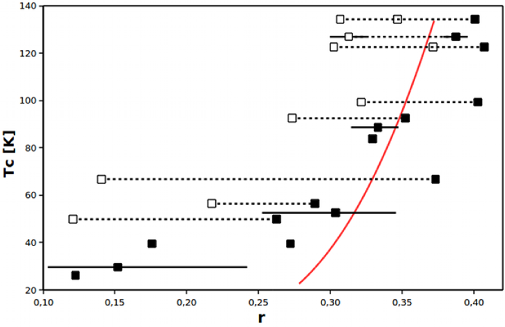
Figure 1: Critical temperature of hole doped cuprates versus band structure parameter $r$ by Pavarini et al. [1]. The theoretical curve is calculated according to Eq. (7) (see text for details).

2 T${}_{\bm{\textsf{c}}}$–r correlation within the s–d theory

Let us introduce a small modification of the $s$ parameter, $\tilde{s}=\displaystyle\frac{t_{\mathrm{sp}}}{t_{\mathrm{pd}}}s.$ Its reciprocal value

$$\frac{1}{\tilde{s}(\epsilon)}=\frac{4t_{\mathrm{pd}}t_{\mathrm{sp}}}{(\epsilon_{\mathrm{s}}-\epsilon)(\epsilon-\epsilon_{\mathrm{p}})},$$ (2)

has an energy denominator typical for the perturbation theory as applied to the secular equation of the generic four-band model

$$\begin{pmatrix}\epsilon_{\mathrm{d}}&0&t_{\mathrm{pd}}s_{x}&-t_{\mathrm{pd}}s_{y}\\ 0&\epsilon_{\mathrm{s}}&t_{\mathrm{sp}}s_{x}&t_{\mathrm{sp}}s_{y}\\ t_{\mathrm{pd}}s_{x}&t_{\mathrm{sp}}s_{x}&\epsilon_{\mathrm{p}}&t_{\mathrm{pp}}s_{x}s_{y}\\ -t_{\mathrm{pd}}s_{y}&t_{\mathrm{sp}}s_{y}&-t_{\mathrm{pp}}s_{x}s_{y}&\epsilon_{\mathrm{p}}\end{pmatrix}\begin{pmatrix}D_{\mathbf{p}}\\ S_{\mathbf{p}}\\ X_{\mathbf{p}}\\ Y_{\mathbf{p}}\end{pmatrix}=\epsilon_{\mathbf{p}}\begin{pmatrix}D_{\mathbf{p}}\\ S_{\mathbf{p}}\\ X_{\mathbf{p}}\\ Y_{\mathbf{p}}\end{pmatrix},$$ (3)

where $\epsilon_{\mathbf{p}}$ is the electron energy for the conducting d-band, $s_{x}=2\sin(p_{x}/2),$ $s_{y}=2\sin(p_{y}/2),$ and the wave function is normalized $D^{2}_{\mathbf{p}}+S^{2}_{\mathbf{p}}+X^{2}_{\mathbf{p}}+Y^{2}_{\mathbf{p}}=1.$ The approximate solution for small hopping amplitudes

$$\begin{pmatrix}D_{\mathbf{p}}\\ S_{\mathbf{p}}\\ X_{\mathbf{p}}\\ Y_{\mathbf{p}}\end{pmatrix}\approx\left(\begin{array}[]{c}1\\ \left(s_{x}^{2}-s_{y}^{2}\right)/4\tilde{s}(\epsilon)\\ \displaystyle\frac{t_{\mathrm{pd}}}{\epsilon-\epsilon_{\mathrm{p}}}s_{x}\\ -\displaystyle\frac{t_{\mathrm{pd}}}{\epsilon-\epsilon_{\mathrm{p}}}s_{y}\end{array}\right),$$ (4)

has a simple interpretation: in the initial approximation we have a pure Cu 3d state with $D_{\mathbf{p}}\approx 1,$ in first approximation we have a linear dependence from the $t_{\mathrm{pd}}$ amplitude on O 2p levels $X_{\mathbf{p}},\;Y_{\mathbf{p}}\propto t_{\mathrm{pd}}$, and finally in second approximation, the amplitude on the Cu 4s orbital $S_{\mathbf{p}}\propto t_{\mathrm{pd}}t_{\mathrm{sp}}$ is included by the second virtual transition proportional to $t_{\mathrm{sp}}$. In short, the Cu 4s amplitude of the conduction band can be phrased as 3d–to–4s–by–2p.

As it was concluded by Pavarini et al. [1] that materials with lower $\epsilon_{\mathrm{s}}$ tend to be those with higher observed values of $T_{\mathrm{c}\,\,max}$. In the materials with higher $T_{\mathrm{c}\,\,max}$ the axial orbital is almost Cu 4s. What is the simplest interpretation of these observations? There is an emerging consensus that superconductivity in cuprates is created by some exchange interaction. The Pavarini et al [1] correlation gives that higher $T_{\mathrm{c}\,\,\mathrm{max}}$ is determined by the highest Cu 4s amplitude $S_{\mathbf{p}}$. Now we have to recall that the most usual 3d–4s intra-atomic exchange has one of the largest amplitudes in condensed matter physics. We also have to point out that transition metal ion-ion exchange integrals $J_{ii},$ which create antiferromagnetism in insulator phase are smaller than intra atomic exchange integral $J_{sd}.$

The intensive investigations of the Kondo effect have demonstrated that the anti-ferromagnetic sign of the two electrons s–d exchange is the rule and the ferromagnetic sign is an exception. Incorporated in the BCS scheme for the calculation of the order parameter $\Xi,$ the anti-ferromagnetic sign gives pairing in singlet channel with momentum dependent gap

$$\Delta_{\mathbf{p}}(T)=\Xi(T)\chi_{\mathbf{p}},\qquad\chi_{\mathbf{p}}\equiv S_{\mathbf{p}}D_{\mathbf{p}}.$$ (5)

This gap is included in the fermion excitation energy

$$E_{\mathbf{p}}\equiv(\eta_{\mathbf{p}}^{2}+\Delta^{2}_{\mathbf{p}})^{1/2},\qquad\eta_{\mathbf{p}}\equiv\epsilon_{\mathbf{p}}-E_{\mathrm{F}},$$ (6)

and for the temperature dependent order parameter $\Xi(T)$ we have the standard BCS equation

$$2J_{\mathrm{sd}}\left<\frac{\chi_{\mathbf{p}}^{2}}{2E_{\mathbf{p}}}\tanh\left(\frac{E_{\mathbf{p}}}{2k_{\mathrm{B}}T}\right)\right>=1,\quad\left<f_{\mathbf{p}}\right>\equiv\int_{0}^{2\pi}\int_{0}^{2\pi}\frac{dp_{x}\,dp_{y}}{(2\pi)^{2}}f(\mathbf{p})$$ (7)

where $\langle\dots\rangle$ denotes momentum–space averaging over the Brillouin zone. For a pedagogical derivation of the BSC gap equation in the present notations see the textbook [2] and references therein. Slightly below the critical temperature where the order parameter disappears $\Xi(T_{\mathrm{c}}-0)=0$ the gap equation reads

$$\quad\left<\frac{\chi_{\mathbf{p}}^{2}}{\eta_{\mathbf{p}}}\tanh\left(\frac{\eta_{\mathbf{p}}}{2k_{\mathrm{B}}T_{\mathrm{c}}}\right)\right>=\frac{1}{J_{\mathrm{sd}}}.$$ (8)

Supposing that $J_{\mathrm{sd}}$, being an intra-atomic process, is weakly temperature dependent we can determent its value using band parameters $\epsilon_{\mathrm{s}},$ $\epsilon_{\mathrm{d}},$ $\epsilon_{\mathrm{p}},$ $t_{\mathrm{sp}},$ $t_{\mathrm{pd}},$ $t_{\mathrm{pp}},$ $E_{\mathrm{F}}$ and known $T_{\mathrm{c}}$. Then we can calculate, for example, the dependence of $T_{\mathrm{c}\,\,\mathrm{max}}$ by position of the Cu 4s levels $\epsilon_{\mathrm{s}}$. One illustrative example is shown in Fig. 2. The almost linear dependence has to have a simple qualitative interpretation. Let us try to reveal this simplicity using the BCS interpolation formula

$$k_{\mathrm{B}}T_{\mathrm{c}}=1.14\,\hbar\omega_{\mathrm{D}}\mathrm{e}^{-1/N(0)V}.$$ (9)

In the present case $\omega_{\mathrm{D}}$ is an energy parameter of order of the bandwidth, $N(E_{\mathrm{F}})$ is electronic density of states per spin at the Fermi level and

$$V=J_{\mathrm{sd}}\frac{4t_{\mathrm{pd}}t_{\mathrm{sp}}}{(\epsilon_{\mathrm{s}}-E_{\mathrm{F}})(E_{\mathrm{F}}-\epsilon_{\mathrm{p}})}=J_{\mathrm{sd}}/\tilde{s}(E_{\mathrm{F}}).$$ (10)

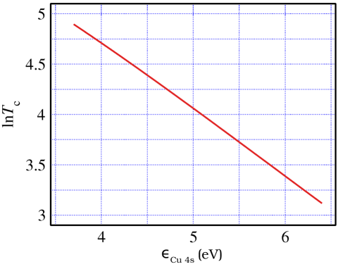
Figure 2: Logarithm of $T_{\mathrm{c}}$ (K) versus $\epsilon_{\text{Cu}\,4\mathrm{s}}$. Science starts with simplicity – the almost linear behavior corresponds to the well-known BCS formulae given by Eqs. (9) and (11).

The interpolation BCS formula gives

$$\ln(T_{\mathrm{c}})\approx\ln(1.14\omega_{\mathrm{D}})-\tilde{s}(E_{\mathrm{F}})/[N(E_{\mathrm{F}})J_{\mathrm{sd}}],$$ (11)

which according to Eq. (2) correlations reported by Pavarini et al. [1] are actually correlations between the critical temperature $T_{\mathrm{c}\,\,\mathrm{max}}$ and the BCS coupling constant $J_{\mathrm{sd}}/\tilde{s}(E_{\mathrm{F}})$. This general correlation is typically perturbed by stripes, inhomogeneities, magnetic phenomena, structural phase transition, apex oxygen, chemical substitution, and many other accessories of HTS cuprates. Nevertheless, they can be clearly seen for all hole doped cuprates. This qualitative agreement gives hope that four-band model with incorporated s–d exchange can become a standard model for superconductivity of cuprates. The key role of the $\tilde{s}(E_{\mathrm{F}})$ parameter reveals why cuprates are unique for reaching high-$T_{\mathrm{c}}$. Imagine that we can easily tune the position of the Cu 4s level $\epsilon_{\mathrm{s}}$. The pre-exponential factor $\omega_{\mathrm{D}}$ is so big that we can easily reach a sauna-temperature superconductivity if $\epsilon_{\mathrm{s}}$ is small enough. Maximal $T_{\mathrm{c}}$ is reached upon 3d–2p–4s hybridization. For the Cu–O duet we have maximal triple coincidence of levels which ensures the success of the CuO₂ plane. For all other combinations of transition metal with a chalcogenide $\tilde{s}$ is much bigger. For 25 years many ways to decrease $\epsilon_{\mathrm{s}}$ were empirically found: apex oxygen, bilayer hopping, pressure, etc. Perhaps only metastable artificial layers are not completely investigated.

3 Computational method

The parent CuO₂ layer is an insulator with a half-filled conduction band. Doping with $\tilde{p}$ holes per Cu atom results in metalization with hole filling $f=\frac{1}{2}+\tilde{p}.$ The optimal doping corresponds to $\tilde{p}_{\mathrm{max}}=0.16$ and $f_{\mathrm{max}}=0.66$. We will use 66% hole filling for all examples in the present work. The Fermi level is determined by the condition

$$f=\left<\theta(\epsilon_{\mathbf{p}}>E_{\mathrm{F}})\right>,\quad\mbox{where}\quad\theta(\epsilon_{\mathbf{p}}>E_{\mathrm{F}})=\begin{cases}1&\text{if }E_{\mathbf{p}}>E_{\mathrm{F}},\\ 0&\text{if }E_{\mathbf{p}}<E_{\mathrm{F}}.\end{cases}$$ (12)

The parameters of the four-band model can be determined by comparison with first-principles electronic structure calculations. For example, using the $\Gamma$ point one can determine the on-site energies $\epsilon_{\mathrm{d}}=\epsilon(p_{x}=0,p_{y}=0)$ for the conduction band. In the present paper we use as an illustration a set of parameters (in eV) similar to Ref. [1]

$$\epsilon_{\mathrm{s}}=5.4,\quad\epsilon_{\mathrm{p}}=-1,\quad\epsilon_{\mathrm{d}}=0,$$ (13)

$$t_{\mathrm{sp}}=2,\quad t_{\mathrm{pd}}=1.5,\quad t_{\mathrm{pp}}=0.2.$$

eV Assuming $T_{\mathrm{c,\,\,max}}=90$ K for $\epsilon_{\mathrm{s}}=5.4$ we obtain, according to Eq. (8), $J_{\mathrm{sd}}=2.44\;\mathrm{eV}.$ Then for so fixed $J_{\mathrm{sd}}$ we can calculate the correlations of $T_{\mathrm{c,\,\,max}}$ with the range parameter

$$r\equiv\frac{1}{2(1+s)}.$$ (14)

Let us discuss briefly our finding. Within the four-band model one can derive an exact equation for constant energy contours

$$-2t(\epsilon)[\cos(p_{x})+\cos(p_{y})]+4t^{\prime}(\epsilon)\cos(p_{x})\cos(p_{y})=q(\epsilon),$$ (15)

where $t(\epsilon),$ $t^{\prime}(\epsilon)$ and $q(\epsilon)$ are polynomial functions of energy. The ratio of the effective intra-layer hopping parameters

$$\frac{t^{\prime}(E_{\mathrm{F}})}{t(E_{\mathrm{F}})}\propto r(E_{\mathrm{F}}),$$ (16)

describes small variations of the shape of the Fermi contour influenced by the position of the Cu 4s level $\epsilon_{\mathrm{s}}$.

4 Conclusions

Electronic structure experts should be proud that after many years of systematic research band calculations have revealed that $T_{\mathrm{c}}$ depends on the Cu 4s level. This numerical experiment is actually the crucial one for understanding the mechanism of HTS. The $r$ parameter is introduced in electronic structure calculations in such a way, that for the first time we have a mechanism of a physical phenomenon possibly revealed by computer.

We advocate a conventional theoretical explanation of the $T_{\mathrm{c}}$-$r$ correlations [1] which has no alternative among other theories of HTS. We have to wait for the appearance of some other descriptions, because this important correlation covers a hole range of HTS. The LCAO model was only a tool for the theoretical analysis of the mechanism of HTS. It should be interesting to determine $S_{\mathbf{p}}$ and $D_{\mathbf{p}}$ directly from partial wave analysis at the muffin spheres directly by the electronic band calculations. The interpolating $\chi_{\mathbf{p}}=S_{\mathbf{p}}D_{\mathbf{p}}$ function can be directly substituted in the BCS gap equation (7) and the equation for $T_{\mathrm{c}}$, Eq. (8). For the cuprates $\chi_{\mathbf{p}}$ well describes the experimental data for the gap anisotropy $\Delta_{\mathbf{p}}$ on the Fermi surface. It remains to be seen if this mechanism is applicable only to cuprates.

The iron-based pnictides are suspected to pursue an Oscar for supporting role. It will be extremely interesting to probe if Eq. (8) can describe the common trends for the $T_{\mathrm{c}}$ and gap anisotropy of ferro-pnictides. In this regards, finally we would like to re-analyze the “boost” that the physics of superconductivity got from the iron pnictides. Very recently, Mazin [3] recalled the Matthias’ rules, well known in the physicists’ folklore: 1) A high symmetry is good; cubic symmetry is the best. 2) A high density of electronic states is good. 3) Stay away from oxygen. 4) Stay away from magnetism. 5) Stay away from insulators. 6) Stay away from theorists.

In order to emphasize the common properties of cuprates and iron pnictides we feel it compelling to rephrase these rules: (1) A high symmetry is good, square symmetry is the best, layered structure ensures empty s-band. (2) Having empty s-band, the Fermi level falls in the narrow d-band which ensures high density of states. (3) The oxygen and pnictide p-orbitals are perfect “go-between” for the transition metal 3d and 4s orbitals. These oxidants create significant 4s polarization of the conduction 3d band. (4) We are just in the epicenter of magnetism; the s-d exchange amplitude which creates the ferromagnetism of iron, possibly creates the superconductivity of iron pnictides and cuprates. (5) Having narrow 3d band in the case of half-filling we observe metal-insulator transition. Transition to insulator phase is a hint for high density of states at the Fermi level for a doped compound. (6) Favorites of great socialists like Lenard, Kapica and Stark, have given similar advice. In order to surmount this weakness it is necessary to remedy the inferiority complex of the band calculators. One Nobel prize is a good initial dose of this treatment. Up to now there is no Nobel prize awarded to computational physics, but the considered in this paper $T_{c}$-$r$ correlations are a typical physical phenomenon whose nature is revealed by numerical calculations. Prediction of an artificial structure with high $\tilde{s}$ parameter, further synthesis by solid-state chemists and measurement of $T_{c}$ may successfully initiate a new direction of intensive research.

In conclusion, we briefly re-state the main property of high-$T_{c}$ superconductivity—the triple coincidence of the d-, s-, and p-levels which ensures big enough BCS coupling constant. This triple coincidence is analogous to the sequence of vernal equinox, full moon, and Sunday (the end of the winter season, the end of the moon month and the end of the week): a triple holiday creating the Great-day. In this sense the high-$T_{c}$ superconductivity is the Easter of condensed matter physics.

The authors are thankful to Prof. Ivan Zhelyazkov for a critical reading of the manuscript and to Alvaro de Rújula for his interest and comments during the scientific conference in memory of Matey Mateev, held in Sofia, 11–12 April 2011.

References

- [1] E. Pavarini, I. Dasgupta, T. Saha-Dasgupta, O. Jepsen, and O. K. Andersen, Band-Structure Trend in Hole-Doped Cuprates and Correlation with , (2001) Phys. Rev. Lett. 87 047003.
- [2] T. M. Mishonov and E. S. Penev (2011) Theory of High Temperature Superconductivity: A Conventional Approach, World Scientific, Singapore, Chap. 2.
- [3] I. Mazin, Superconductivity gets an iron boost, (2010) Nature 464, 183–186.